Developing machine-learned potentials to simultaneously capture the dynamics of excess protons and hydroxide ions in classical and path integral simulations

Abstract

The transport of excess protons and hydroxide ions in water underlies numerous important chemical and biological processes. Accurately simulating the associated transport mechanisms ideally requires utilizing ab initio molecular dynamics simulations to model the bond breaking and formation involved in proton transfer and path-integral simulations to model the nuclear quantum effects relevant to light hydrogen atoms. These requirements result in a prohibitive computational cost, especially at the time and length scales needed to converge proton transport properties. Here, we present machine-learned potentials (MLPs) that can model both excess protons and hydroxide ions at the generalized gradient approximation and hybrid density functional theory levels of accuracy and use them to perform multiple nanoseconds of both classical and path-integral proton defect simulations at a fraction of the cost of the corresponding ab initio simulations. We show that the MLPs are able to reproduce ab initio trends and converge properties such as the diffusion coefficients of both excess protons and hydroxide ions. We use our multi-nanosecond simulations, which allow us to monitor large numbers of proton transfer events, to analyze the role of hypercoordination in the transport mechanism of the hydroxide ion and provide further evidence for the asymmetry in diffusion between excess protons and hydroxide ions.

I Introduction

Water’s ability to autoionize and efficiently transport its ionization products—excess protons and hydroxide ions—through its hydrogen bond network is a fundamental characteristic that underlies multiple processes ranging from acid-base chemistry to the operation of proton exchange membrane fuel cells Peighambardoust, Rowshanzamir, and Amjadi (2010) and voltage-gated proton channels in biological cell membranes DeCoursey (2018). Excess protons and hydroxide ions are known to diffuse via structural (Grotthuss-like) mechanisms Marx (2006), which involve the making and breaking of chemical bonds through a series of proton transfer reactions between neighboring water molecules. These structural diffusion mechanisms allow both species to diffuse much faster than water itself and are intricately linked to the structure and dynamics of the hydrogen bonds that solvate proton defects in water Hassanali et al. (2013). Excess protons and hydroxide ions thus exhibit different diffusion rates in water due to their different solvation motifs, and nuclear magnetic resonance (NMR) Halle and Karlström (1983a, b) and conductivity Halle and Karlström (1983a); Weingärtner and Chatzidimttriou-Dreismann (1990); Sluyters and Sluyters-Rehbach (2010) measurements have shown that excess protons diffuse $\sim$1.8 times faster than hydroxide ions at room temperature. The need for a deeper understanding of the complex molecular structures and motions that lead to these diffusion mechanisms and the differences between the diffusion rates of excess protons and hydroxide ions has led to extensive theoretical studies Tuckerman et al. (1995a, b); Agmon (1995); Marx et al. (1999); Marx, Tuckerman, and Parrinello (2000); Vuilleumier and Borgis (1999); Day, Schmitt, and Voth (2000); Tuckerman, Marx, and Parrinello (2002); Agmon et al. (2016). However, due to the reactive nature of the defects, which necessitate a quantum mechanical treatment of the electrons to allow chemical bonds to be made and broken during the simulation, and their low mass, which requires consideration of nuclear quantum effects, resolving the interplay of these physical effects and how they are engendered in the diffusion mechanism has remained a subject of significant debate.

Early studies of proton transport in water invoked symmetry between the hydronium (H₃O⁺) and hydroxide (OH^-) ions Hückel (1928); Eigen (1964); Stillinger (1978); Zatsepina (1972); Schiöberg and Zundel (1973); Librovich, Sakun, and Sokolov (1979); Khoshtariya and Berdzenishvili (1992); Agmon (2000) to suggest a framework where the structural transport mechanism of hydroxide ions could be inferred directly as the inverse of the corresponding mechanism for excess protons. However, it has since become clear that the two ions follow distinct proton transfer pathways, a phenomenon that is commonly attributed to differences in their solvation patterns Hückel (1928); Eigen (1964); Stillinger (1978); Zatsepina (1972); Schiöberg and Zundel (1973); Librovich, Sakun, and Sokolov (1979); Khoshtariya and Berdzenishvili (1992); Agmon (2000). In particular, OH^- can exhibit a hypercoordinated configuration where it accepts four hydrogen bonds Tuckerman, Marx, and Parrinello (2002), whereas the H₃O⁺ ion can only donate three. This effect underscores the importance of water’s complex hydrogen bond network in facilitating and ultimately influencing the rate of proton transport.

One of the most commonly invoked approaches to simulate the bond making and breaking that accompanies proton transfer in the structural diffusion of proton defects has been to perform computationally costly ab initio molecular dynamics (AIMD) simulations, where forces are obtained on the fly from electronic structure calculations. In addition, due to the light hydrogen nuclei involved, capturing a complete picture of the transport of proton defects requires including nuclear quantum effects (NQE) such as tunnelling and zero-point energy. Ab initio path-integral simulations include both of these effects and have been shown to be vital for the accurate description of the structure and transport of both H₃O⁺ and OH^- Tuckerman, Marx, and Parrinello (2002); Marx (2006); Agmon (2000); Napoli, Marsalek, and Markland (2018). While imaginary-time path-integral simulations exactly include NQEs for structural properties, path-integral-based methods such as centroid molecular dynamics (CMD) Cao and Voth (1994); Jang and Voth (1999) and ring polymer molecular dynamics (RPMD) Craig and Manolopoulos (2004); Habershon et al. (2013) have been shown to provide reliable approximate quantum dynamics for condensed phase systems. However, 30-100 replicas of a classical system are usually needed for path-integral simulations of aqueous systems at room temperature when using the most commonly employed second-order path integral discretization approach Ceriotti et al. (2016), increasing the computational cost by at least 30 times compared to AIMD simulations with classical nuclei. As such, ab initio path-integral molecular dynamics (AI-PIMD) simulations of the lengths required to sample many proton transfer events (on the order of nanoseconds) and hence reliably converge proton transport properties have traditionally been prohibitively costly. Recent path integral acceleration approaches Markland and Ceriotti (2018) such as those that combine multiple time scale molecular dynamics Tuckerman, Berne, and Martyna (1992) and ring polymer contraction Markland and Manolopoulos (2008a, b); Fanourgakis, Markland, and Manolopoulos (2009); Marsalek and Markland (2016); Kapil, VandeVondele, and Ceriotti (2016) have made these timescales accessible for AI-PIMD simulations of 100’s of picoseconds for systems of 300-500 atoms Marsalek and Markland (2017); Napoli, Marsalek, and Markland (2018), albeit still at a formidable computational cost.

The recent ability to perform condensed-phase simulations that combine electronic structure methods—most commonly density functional theory (DFT)—with path-integral methods has led to the identification of failures of the electronic structure treatments that were previously obfuscated when the nuclei were treated classically. Since the zero-point energy in the OH stretch provides additional energy equivalent to raising the temperature of that coordinate by $\sim$2000 K, performing AI-PIMD simulations of liquid water explores much higher-energy regions of the potential energy surface, such as long chemical bond extensions, which causes significant issues when lower-tier generalized gradient approximation (GGA) exchange correlation functionals are employed Marsalek and Markland (2016); Ceriotti et al. (2016); Gasparotto, Hassanali, and Ceriotti (2016); Marsalek and Markland (2017). For example, when the nuclei are treated classically, spurious self-interaction in the revPBE-D3 GGA functional, which leads to an overly weak OH covalent bond, is fortuitously largely canceled out by the exclusion of NQEs, and hence the reintroduction of NQEs worsens the GGA functional’s description of water Marsalek and Markland (2017). While it has been shown that this deficiency can be alleviated by combining PIMD calculations with more costly hybrid functionals such as revPBE0-D3 Marsalek and Markland (2017); Cheng et al. (2019), the charged nature of proton defects is likely to exacerbate these issues further. Given the number of vital chemical processes which involve proton defects in nanoconfinement or at interfaces that typically require system sizes of more than 500 atoms and even longer timescales (multi-nanosecond) to average over the heterogeneity of the environment, performing converged AI-PIMD simulations of proton defects in these systems is likely to be impractical for the foreseeable future.

Machine-learned potentials (MLPs) have recently emerged as a compelling alternative to ab initio simulations Behler and Parrinello (2007); Behler (2011, 2014). By training MLPs on the energies and/or forces obtained from ab initio calculations on a small number of suitably selected configurations (typically on the order of 1000s), MLPs have been shown to be able to interpolate, and in certain cases extrapolate, the ab initio potential energy surface over a wide range of conditions. While MLPs that can successfully model the reactive dynamics of protonated water clusters Natarajan, Morawietz, and Behler (2015); Schran, Behler, and Marx (2019) and NaOH solutions Hellström and Behler (2016); Hellström, Ceriotti, and Behler (2018) have previously been developed, they have not aimed to capture the behavior of both H₃O⁺ and OH^- concurrently. Here, we develop and introduce a training set sampled from ab initio simulations of excess protons, hydroxide ions, and proton-hydroxide recombination events and use it to train MLPs at the GGA (revPBE-D3) and hybrid (revPBE0-D3) levels of theory. We show that these MLPs can be used to simultaneously capture the properties of both types of proton defects in water, thus allowing the study of excess proton diffusion, hydroxide ion diffusion, water autoionization, and defect recombination processes. We utilize these MLPs to run both classical and path-integral AIMD simulations, allowing us to assess the role of different tiers of treatment of the electronic structure and NQEs in determining the mechanism of proton transport.

II Building the Machine-Learned Potential

II.1 Training Set Creation

We utilized a training set of 37102 configurations, prepared by combining 4594 bulk water configurations randomly sampled from a previously reported dataset Morawietz et al. (2018) with 32508 new configurations containing proton defects. The added proton defect configurations consist entirely of neutral frames of water molecules that contain a proton defect pair (both an excess proton and hydroxide ion). We do not include frames of water molecules containing the excess proton or hydroxide ion in isolation because such configurations require an opposite homogeneous background charge to neutralize the simulation box, which leads to box energies that vary depending on the box volume and Ewald summation parameters. The resulting variation in the energies complicates the fitting of an MLP, and hence we concentrate on fitting the MLP to the more physical neutral configurations where both the excess proton and hydroxide ion are present.

To prepare the training configurations that incorporate both excess protons and hydroxide ions, we selected frames from a revPBE-D3 AIMD trajectory of the hydroxide ion in water, identified the farthest water molecule from the OH^-, and added an excess proton to it, thereby neutralizing the frame. We used these frames to initialize classical and quantum revPBE-D3 AIMD trajectories with the aim of simulating proton defect recombination. From the resulting trajectories, we sampled configurations from the subset of frames where the proton defects had not recombined. Configurations were separately sampled to obtain a training set with near uniform distributions of the proton sharing coordinate ($\delta$, see section III.2 for definition) for the excess proton and hydroxide ion. Finally, similar to the configurations in the starting water dataset Morawietz et al. (2018), $\sim$67% of the defect-separated frames were augmented by randomly displacing atoms to create configurations with higher forces, which served to improve model stability. The details of the training set are summarized in SI Table III.

Once the training and validation set configurations were obtained, their energies and forces were re-evaluated at the revPBE Perdew, Burke, and Ernzerhof (1996); Zhang and Yang (1998) and revPBE0 Adamo and Barone (1999); Goerigk and Grimme (2011) levels of DFT with D3 dispersion Grimme et al. (2010) using the CP2K program VandeVondele et al. (2005); Kühne et al. (2020). Atomic cores were represented via the Godecker-Tetter-Hutter pseudopotentials Goedecker, Teter, and Hutter (1996). We employed the hybrid Gaussian and plane wave density functional scheme Lippert, Hutter, and Parrinello (1997), where the Kohn-Sham orbitals were expanded in the larger molecular optimized (MOLOPT) VandeVondele and Hutter (2007) TZV2P basis set, and an auxiliary plane-wave basis was used to represent the density with a cutoff of 400 Ry for the revPBE-D3 calculation and 900 Ry for revPBE0-D3. Due to the relatively compact size of our training set, we are able to evaluate all of the configurations using a more accurate basis set that would be exceptionally computationally costly to use in AIMD simulations.

II.2 Architecture and Training of the Machine-Learned Potential

Our revPBE-D3 MLP was fit using the RuNNer package Behler (2016), while the revPBE0-D3 MLP was fit using the n2p2 package Singraber et al. (2021). We employed Behler-Parrinello neural networks Behler and Parrinello (2007); Morawietz et al. (2016) with two hidden layers containing 25 nodes each and an input layer containing 56 and 46 nodes for the H and O neural networks respectively. Chemical environments were described by radial and angular atom-centered symmetry function descriptors Behler (2011) with a cutoff of 6.35 Å. We employed a 90/10 train/validation split, with 33425 configurations in the training set and 3677 configurations in the validation set. Training was done over 20 epochs, and MLP weights were fit to forces and energies. The final energy and force validation errors were 0.433 meV/atom and 65.8 meV/Å for the GGA MLP and 0.485 meV/atom and 39.4 meV/Å for the hybrid MLP respectively.

III Simulation Details

III.1 MD Simulations

We performed classical and path integral simulations of both the excess proton and hydroxide ion in water under NVT conditions at T=300 K. The potential energy surfaces were described by MLPs trained on configurations from revPBE Perdew, Burke, and Ernzerhof (1996); Zhang and Yang (1998) (GGA) and revPBE0 Adamo and Barone (1999); Goerigk and Grimme (2011) (hybrid) AIMD simulations with D3 dispersion Grimme et al. (2010) (see subsections II.1 and II.2), yielding four simulation protocols: classical GGA, classical hybrid, quantum GGA, and quantum hybrid. For all simulation protocols, we used a cubic box of length 15.66 Å with periodic boundary conditions. The simulation box contained 128 water molecules from which one proton was either removed, creating a hydroxide ion, or to which a proton was added, yielding an excess proton and resulting in a proton defect concentration in both cases of 0.43 M. To investigate finite-size effects, two sets of additional classical GGA trajectories were run in cubic boxes of lengths 19.73 Å and 24.86 Å. In these one proton was added (excess proton) or removed (hydroxide ion) from simulations consisting of 256 and 512 water molecules, yielding proton defect concentrations of 0.22 M and 0.11 M respectively.

Classical MLP simulations were run with a 0.5 fs time step using the LAMMPS package Thompson et al. (2022), which employed n2p2 Singraber, Behler, and Dellago (2019) to incorporate the MLP. A stochastic velocity rescaling (SVR) thermostat Bussi, Donadio, and Parrinello (2007) with a time constant of 1 ps was used to sample the canonical ensemble. For both the classical GGA and classical hybrid simulation protocols, we ran 107$\times$ and 70$\times$ 200-ps trajectories of the excess proton and hydroxide ion respectively at a box size of 15.66 Å. This resulted in 21.4 ns of acid trajectory and 14 ns of base trajectory for each of the classical GGA and classical hybrid simulation protocols, with frames that were recorded every 2 fs. For the bigger cell sizes (boxes of lengths 19.73 Å and 24.86 Å), we ran $\sim$100$\times$ and $\sim$80$\times$ 200-ps classical GGA trajectories of both the acid and base, resulting in 20 ns and 16 ns of trajectory respectively.

Path-integral MLP simulations were run with a 0.25 fs time step by employing the i-PI program Ceriotti, More, and Manolopoulos (2014); Kapil et al. (2019), which used the LAMMPS package Thompson et al. (2022) (with n2p2 Singraber, Behler, and Dellago (2019) used for the MLP) to compute energies and forces. The quantum path-integral simulations were performed via thermostatted ring polymer dynamics (TRPMD) Craig and Manolopoulos (2004); Habershon et al. (2013); Rossi, Ceriotti, and Manolopoulos (2014) using 32 beads that were thermostatted with the path integral Langevin equation (PILE) Ceriotti et al. (2010). Under this scheme, ring polymer internal modes with frequency $\omega_{k}$ were subjected to a Langevin thermostat with friction $\gamma_{k}=2\lambda\omega_{k}$ and $\lambda=0.5$. For the quantum GGA and quantum hybrid simulation protocols, we ran 10 $\times$ 200-ps trajectories of both the excess proton and hydroxide ion, resulting in 2 ns of quantum trajectories for each combination of quantum simulation protocol and proton defect. Like in the classical case, frames were recorded every 2 fs.

We also performed classical GGA AIMD simulations of the excess proton and hydroxide ion in water under NVT conditions at T=300 K to serve as a benchmark for our MLP simulations. The AIMD simulations were run under periodic boundary conditions in cubic boxes of length 12.42 Å containing 64 water molecules from which a proton was removed or to which a proton was added. We employed the i-PI program Ceriotti, More, and Manolopoulos (2014); Kapil et al. (2019) and its MTS Tuckerman, Berne, and Martyna (1992) implementation Kapil, VandeVondele, and Ceriotti (2016) to propagate the nuclei. The full and reference forces were evaluated using the CP2K program VandeVondele et al. (2005); Kühne et al. (2020). Full forces were computed at the revPBE Perdew, Burke, and Ernzerhof (1996); Zhang and Yang (1998) level of DFT with D3 dispersion Grimme et al. (2010). Atomic cores were represented via the Godecker-Tetter-Hutter pseudopotentials Goedecker, Teter, and Hutter (1996). We employed the hybrid Gaussian and plane wave density functional scheme Lippert, Hutter, and Parrinello (1997), where the Kohn-Sham orbitals were expanded in the TZV2P basis set, and an auxiliary plane-wave basis with a cutoff of 400 Ry was used to represent the density. The self-consistent field cycle was converged to an electronic gradient tolerance of $\epsilon_{\mathrm{SCF}}=5\times 10^{-7}$ using the orbital transformation method VandeVondele and Hutter (2003) with the initial guess provided by the always stable predictor-corrector extrapolation method Kolafa (2003); Kühne et al. (2007) at each AIMD step. Reference forces for the MTS were evaluated at the SCC-DFTB level in periodic boundary conditions using Ewald summation for electrostatics. The parametrizations for H and O atoms provided by CP2K were used and the D3 dispersion correction was added. The AIMD simulations were performed using an MTS propagator with the full force evaluated with a time step of 2.0 fs and the reference force with a time step of 0.5 fs. The SVR thermostat was employed with a time constant of 1 ps. We obtained total simulation times of 718 ps divided over 2 trajectories for the acid and 800 ps divided over 4 trajectories for the base.

III.2 Trajectory Analysis

A great deal of the results presented here arise from tracking the proton defect, which was identified at each frame by assigning every H atom to its nearest O and picking out the triply coordinated O atom (H₃O⁺) in the excess proton trajectories and the singly coordinated O atom (OH^-) in the hydroxide ion trajectory. The atoms that make up the proton defect are referred to as O^∗ and H^∗ throughout this manuscript. Occasionally, highly transient water autolysis events (2H₂O $\rightarrow$ H₃O⁺ + OH^-) would occur, forming excess ($>$1) proton defects at their respective frame. These events were rare, ranging from a maximum of 0.044% of all frames for the quantum GGA excess proton trajectories to a minimum of 6.5$\times$ 10^-5% of all frames for the classical hybrid excess proton trajectories. The ions resulting from these events were disregarded in our analysis, which instead focused on tracking the movement of the proton defect present at t=0. We defined the hydrogen bond geometrically as an atomic triplet O_d–H_d…O_a (where O_d and H_d are covalently bonded donor atoms and O_a is an acceptor atom) with $|$O_dO_a$|$ $\leq$ 3.5 Å and $\angle$ O_aO_dH_d $\leq$ 30 $\degree$ Luzar and Chandler (1996).

We computed mean square displacements (MSDs) for both the proton defect and water (O atoms) in our trajectories via the formula:

$$\mathrm{MSD}(\Delta t)=\langle|\mathbf{r}(t_{0}+\Delta t)-\mathbf{r}(t_{0})|^{2}\rangle,$$ (1)

where $\langle\rangle$ is an ensemble average computed over all time origins $t_{0}$ and all relevant atoms. Diffusion coefficients were obtained by performing a linear fit to the MSD in the range 4 ps $\leq\Delta t\leq$ 20 ps and dividing it by $2d=6$, where $d$ refers to the 3 dimensions of the simulation. We performed finite-size corrections for the water diffusion coefficient according to Yeh and Hummer (2004):

$$D(\infty)=D(L)+\frac{\xi k_{\mathrm{B}}T}{6\pi\eta L},$$ (2)

where $L$ is the length of the simulation cell, $k_{\mathrm{B}}$ is the Boltzmann constant, and $T$ is the temperature, $\xi=2.837297$ is based on the cubic geometry of the simulation cell, and $\eta=0.8925\times 10^{-3}$ Pa s is the experimental shear viscosity.

For the TRPMD simulations, we used the positions of the centroids to compute the MSD for the diffusion coefficient (which is a property of the long-time slope and hence gives the same result as using the beads); all other observables were calculated from the positions of the individual beads.

IV Validation of the Machine-Learned Potential

We begin by evaluating how well classical molecular dynamics ran with our GGA-trained MLP reproduces observables from classical GGA ab initio molecular dynamics (AIMD) simulations. We benchmark on classical GGA since it has the lowest computational cost of the electronic structure and dynamics approaches presented in this study, and hence we can generate relatively long (718 ps for the acid and 800 ps for the base) AIMD trajectories with minimal statistical noise. Thus the discrepancies between the MLP and AIMD simulations in obtaining the properties of the systems discussed below, with the exception of the diffusion coefficients, do not arise from statistical sampling errors but rather either from errors in the MLP or due to the fact that the MLP was fit to a larger and more accurate MOLOPT basis set which was too computationally expensive to use for our long AIMD simulations. As shown in Fig. 5, even nanosecond-long trajectories lead to significant statistical error bars in the diffusion coefficients, so benchmarking the MLP on this property using AIMD is extremely challenging. This is one of the main motivations for the development of the MLP, which allows for the generation of trajectories that are long enough to converge this important property.

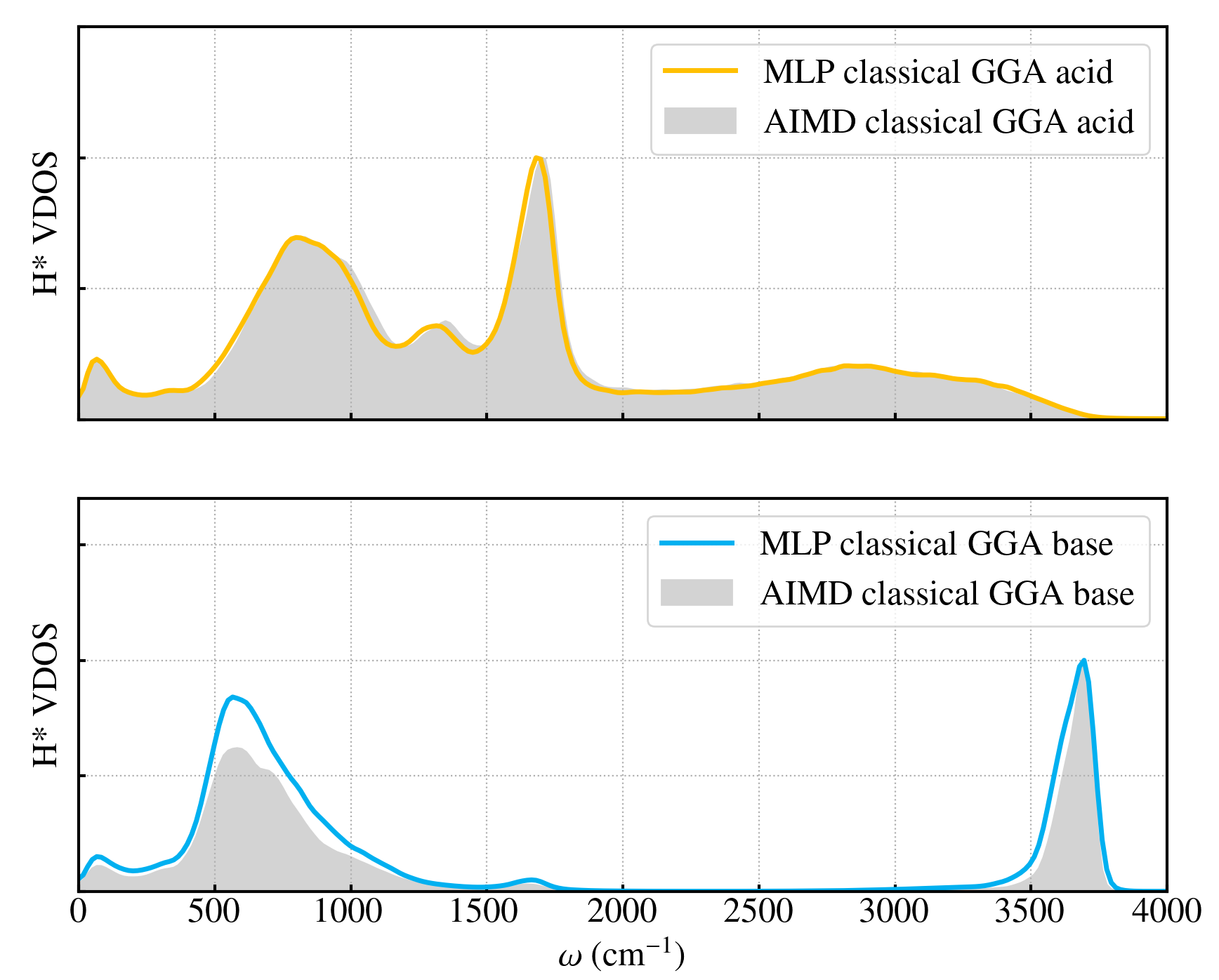
Figure 1: Comparison of the H^∗ VDOS for revPBE-D3 AIMD and the revPBE-D3-trained MLP trajectories. The top panel shows this comparison for acid trajectories, while the bottom panel shows the comparison for base trajectories.

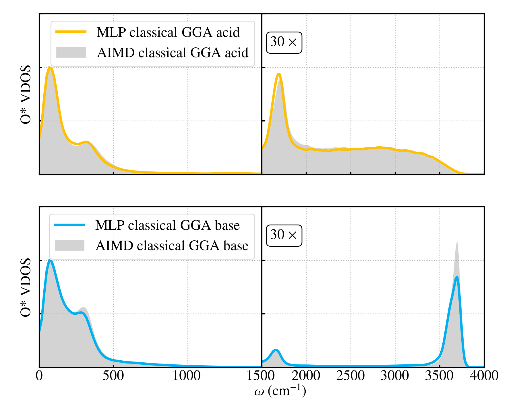
Figure 2: Comparison of the O^∗ VDOS for revPBE-D3 AIMD and the revPBE-D3-trained MLP trajectories. The top panel shows this comparison for acid trajectories, while the bottom panel shows the comparison for base trajectories.

We consider the vibrational density of states (VDOS) for H^∗ and O^∗—i.e., the H and O atoms that make up the H₃O⁺ and OH^- defects in simulations with an excess proton and a hydroxide ion respectively (see Sec. III.2)—shown in Figs. 1 and 2 respectively. These VDOS focus on the reactive defects and thus provide a stricter test of the MLP than the VDOS of all H and O atoms in the system (see SI Sec. II), most of which are bound to water molecules. For the excess proton, the MLP manages to accurately reproduce all features of the H^∗ VDOS that are characteristic of the reactive defects Fournier et al. (2018); Agmon et al. (2016). These include the blue-shifted librational band at $\sim$800 cm^-1, the broadened bending mode peak at $\sim$1600 cm^-1, the broad absorption band between the bend and the OH stretch region (2000-3600 cm^-1), and a peak around $\sim$1250 cm^-1 which has previously been assigned to a Zundel-like proton shuttling motion Headrick, Bopp, and Johnson (2004); Headrick et al. (2005); Asmis et al. (2003). The H^∗ VDOS for the hydroxide ion has fewer features: a librational band at $\sim$600 cm^-1, a comparatively smaller bending mode peak at $\sim$1600 cm^-1, and an OH stretch peak at $\sim$3600 cm^-1 that is sharper than that of pure liquid water Roberts et al. (2009); Agmon et al. (2016). While the MLP manages to accurately reproduce the frequencies of the features, it overestimates the amplitude of the librational band ($\sim$600 cm^-1) for the hydroxide ion. Figure 2 shows quantitative agreement in the O^∗ VDOS between the MLP and AIMD trajectories, with the much weaker bending mode peaks ($\sim$1600 cm^-1 for both the excess proton and hydroxide ion), the absorption band (2000-3600 cm^-1 for the excess proton), the stretch signal ($\sim$3600 cm^-1 for the hydroxide ion) and low-frequency features ($<$ 500 cm^-1) being faithfully reproduced by the MLP.

In Figures 3 and 4, we evaluate how well the GGA-trained MLP reproduces the AIMD free energy along the proton sharing coordinate. As illustrated in Figs. 3 and 4, $\delta=d_{\mathrm{O^{\prime}H^{*}}}-d_{\mathrm{O^{*}H^{*}}}$ for the excess proton and $\delta=d_{\mathrm{O^{*}H^{\prime}}}-d_{\mathrm{{O^{\prime}H^{\prime}}}}$ for the hydroxide ion, where $d$ denotes the distance between the respective atoms. O^∗ and H^∗ are the defect atoms defined above, while O^′ and H^′ are atoms in the first solvation shell of the charge defect. For the excess proton simulations, of the $\delta$ values from the three H^∗ atoms connected to O^∗, only the lowest was used, and for the hydroxide ion simulation, the $\delta$ values were calculated based only on the H^′ closest to O^∗. The free energy along the delta coordinate $\Delta F(\delta)=-k_{\mathrm{B}}T\ln P(\delta)$ was calculated from the resulting $\delta$ probability distribution, $P(\delta)$. The two free energy minima along the proton sharing coordinate, $\delta$, thus correspond to the covalent bonding of the hydrogen atom to one or the other oxygen atom, and the height of the free energy barrier between the two minima is located at $\delta$=0 due to the symmetry of the coordinate.

Figures 3 and 4 show that the MLP simulations accurately reproduce both the positions of the free energy minima and height of the free energy barrier at $\delta=0$, $\delta F(\delta=0)$, obtained from AIMD, with the MLP overestimating it by 0.02 kcal/mol for the acid and underestimating it by 0.12 kcal/mol for the base. At 300 K, these errors correspond to 0.03 and 0.2 $k_{\mathrm{B}}T$ respectively, are much smaller than the thermal energy in the system, and are completely dwarfed by the zero-point energy along these coordinates as discussed further in Sec. V.

To further validate that the structural and dynamical properties of the excess proton and hydroxide ion in liquid water are captured by our GGA MLP, we show in SI Sec. I that the MLP also quantitatively reproduces the AIMD O^∗-O, O^∗-H, and H^∗-H radial distribution functions for both simulations. Finally, the MLP trajectories yield O^∗ diffusion coefficients of 8.04 $\times$ 10^-9 and 4.95 $\times$ 10^-9 m²/s for the excess proton and hydroxide ion respectively, which compare favorably to corresponding AIMD values of 9.87 $\times$ 10^-9 and 3.13 $\times$ 10^-9 m²/s. As discussed in Sec. V, the slow convergence of the proton defect diffusion coefficient with simulation time is such that the difference between the MLP and AIMD diffusion coefficients can be accounted for by statistical uncertainty. This is further illustrated in SI Fig. 7.

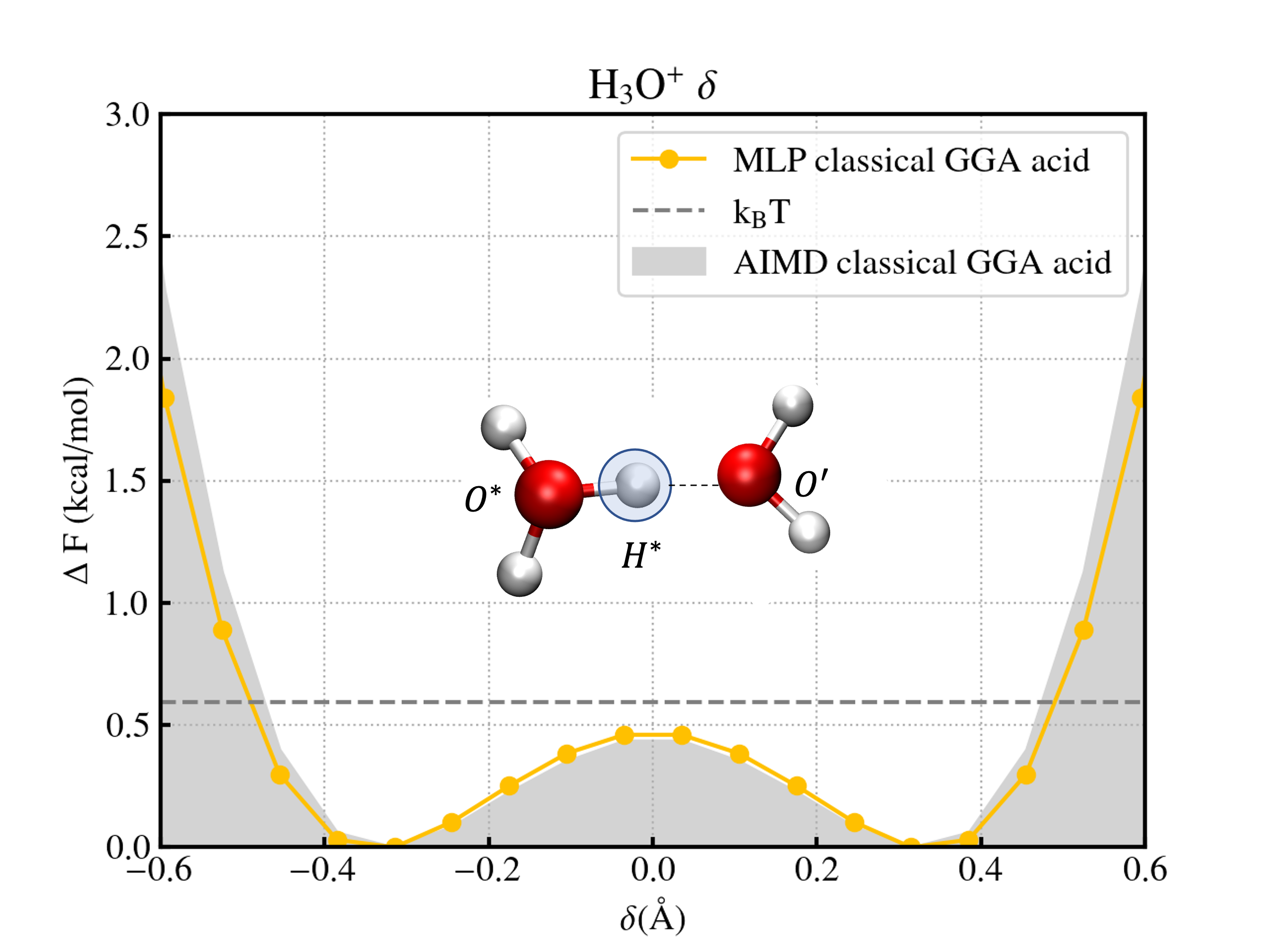
Figure 3: Comparison of the proton transfer free energy barrier along the proton sharing coordinate, $\delta=\mathrm{O^{\prime}H^{*}-O^{*}H^{*}}$, for revPBE-D3 AIMD and revPBE-D3-trained MLP acid trajectories. We only consider the H^∗ with the lowest $\delta$ value at each frame.

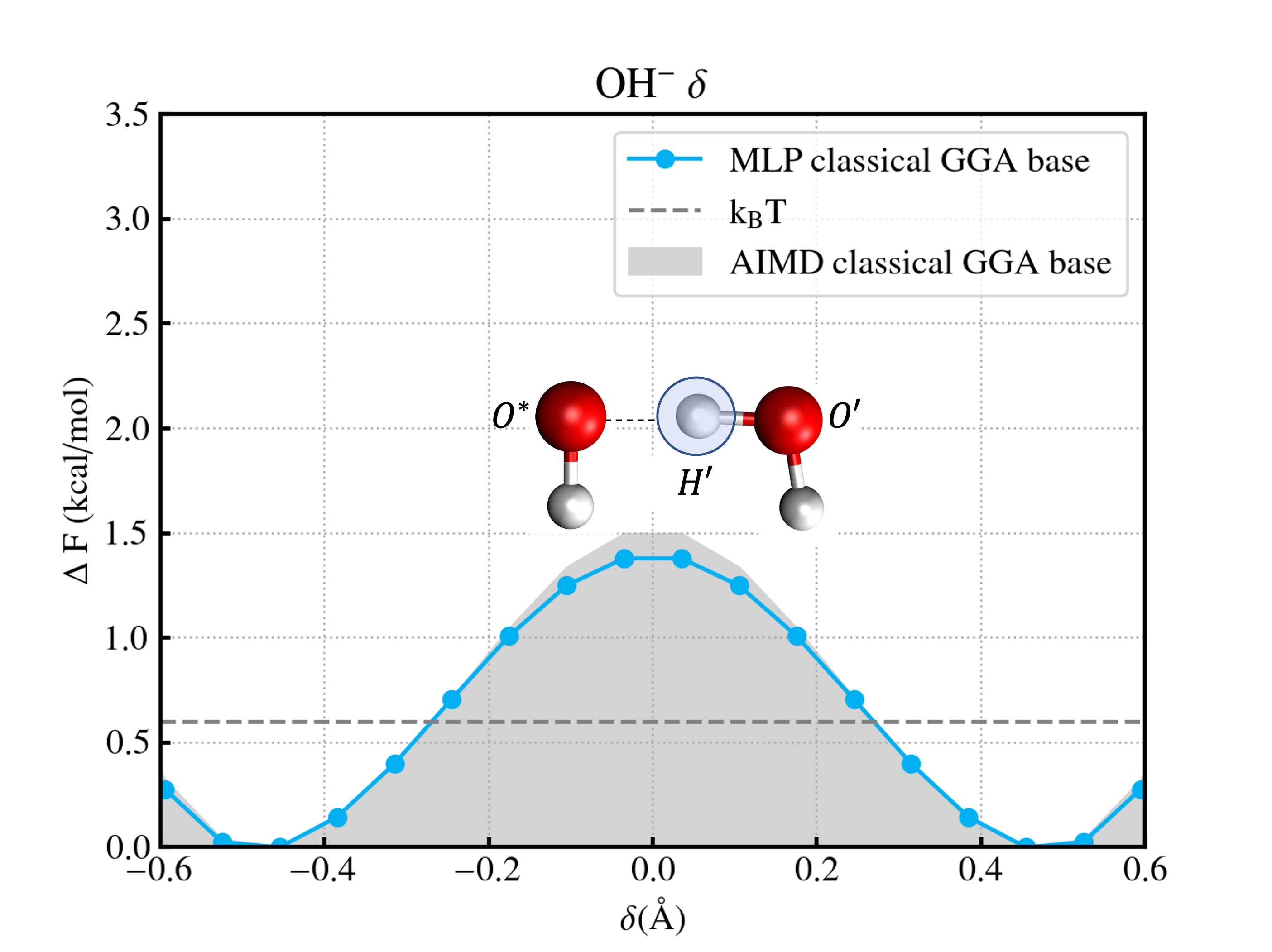
Figure 4: Comparison of the proton transfer free energy barrier along the proton sharing coordinate, $\delta=\mathrm{O^{*}H^{\prime}-O^{\prime}H^{\prime}}$, for revPBE-D3 AIMD and revPBE-D3-trained MLP base trajectories. We only consider the H^′ closest to the O^∗ at each frame.

V Results

Having established the accuracy of the GGA MLP trained on ab initio data in the previous section, we now investigate the properties of excess protons and hydroxide ions in water at the GGA and hybrid levels of DFT with and without nuclear quantum effects. Due to the low computational cost of evaluating MLPs, we investigate properties (such as the proton defect diffusion coefficients) that require multiple nanoseconds of simulation to reliably converge. The importance of using such long simulations is illustrated in Fig. 5, which shows the distribution of diffusion coefficients obtained from 50 ps, 100 ps, and 200 ps trajectory segments derived from subdividing our total of 20 ns of revPBE-D3 (GGA) MLP trajectory. A single simulation performed on a 50 ps, 100 ps, or 200 ps timescale would thus correspond to picking a single realization from these distributions (with each diffusion coefficient corresponding to the linear fit to one of the MSD curves shown in SI Figures 9 and 10, as detailed in Section III.2). As one can see, even with a 200 ps simulation, a time longer than that in many previous AIMD studies of proton defects, the wide distribution of diffusion coefficients that can be obtained does not allow one to reliably distinguish between the higher expected diffusion coefficient of an excess proton and the lower one expected for the hydroxide ion. This emphasizes the need for multiple-nanosecond simulations to comment on the relative transport rates of the excess proton and hydroxide ion in liquid water.

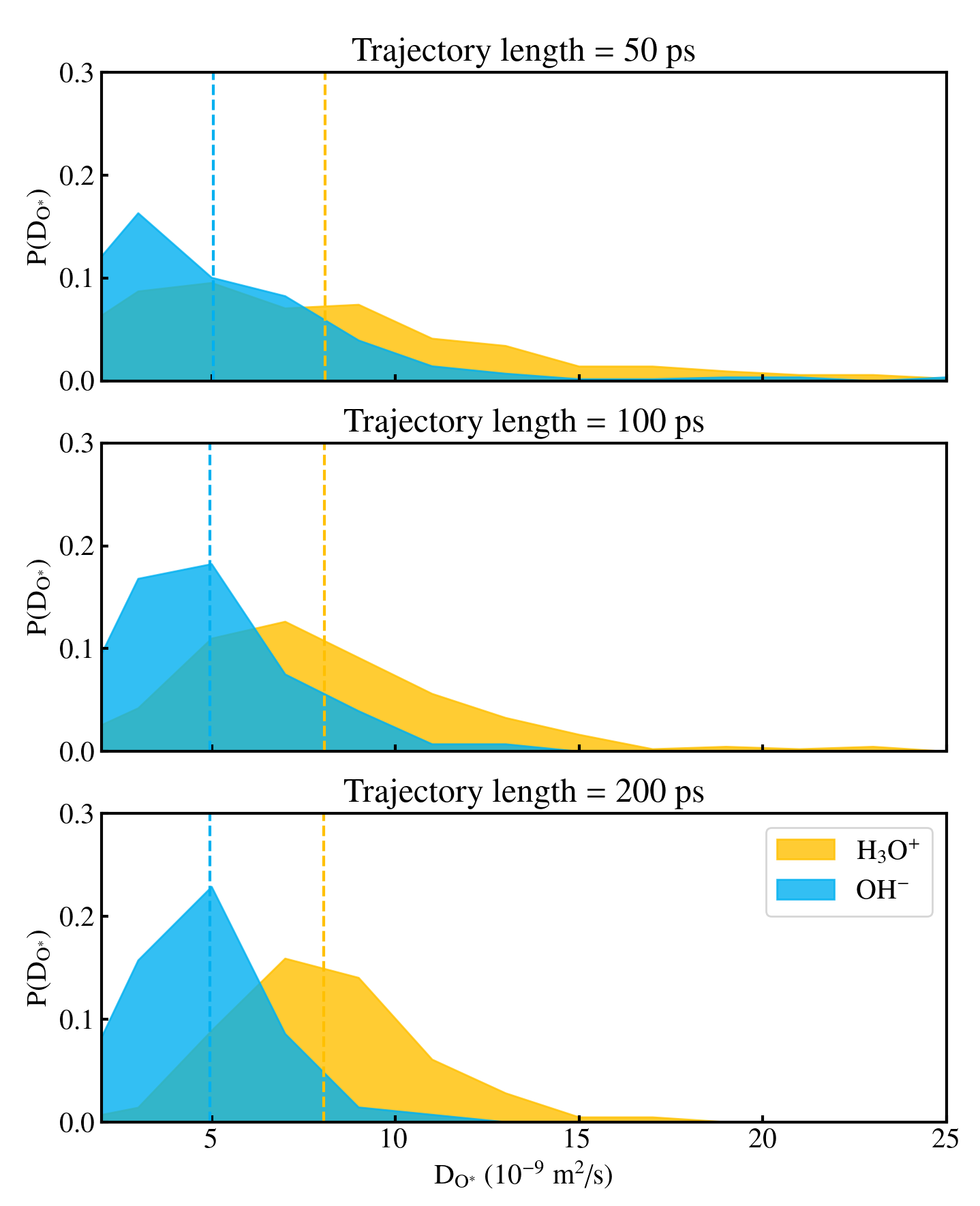
Figure 5: Proton defect diffusion coefficient distributions (P(D${}_{\mathrm{O^{*}}}$)) of the MLP GGA simulations computed at different trajectory lengths, with the corresponding means displayed as dashed lines. The degree of separation between the D${}_{\mathrm{O^{*}}}$ distributions for the acid and base increases with the trajectory length, underscoring the importance of computing D${}_{\mathrm{O^{*}}}$ values from trajectories that are at least hundreds of picoseconds long.

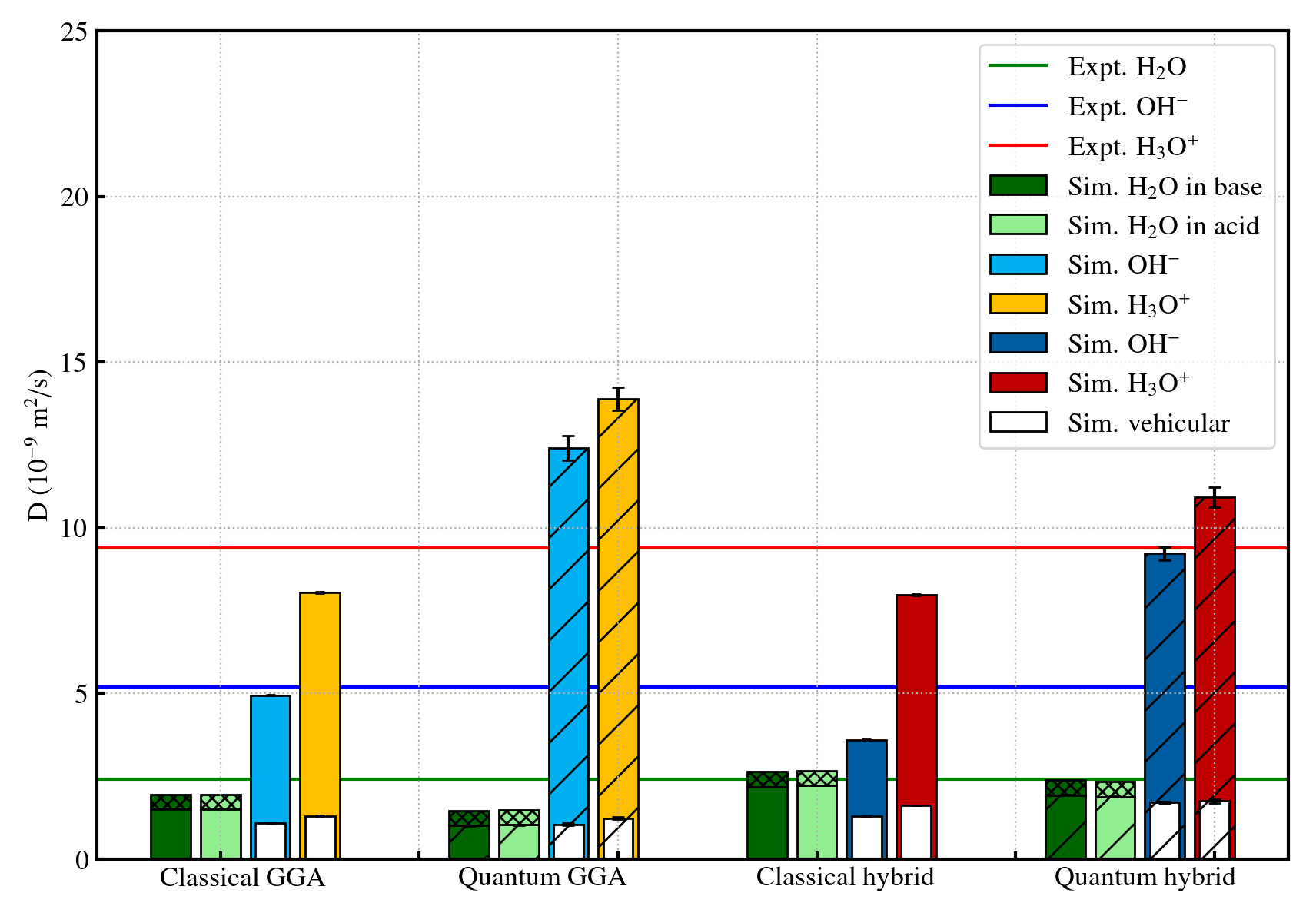
Figure 6: Acid and base diffusion coefficients calculated from the MLP trajectories. We report six values for each MLP run: the molecular diffusion coefficient of water (measured by tracking O atoms) in the acid and base, the proton defect diffusion coefficient (measured by tracking O^∗) in the acid and base, and the vehicular component of the proton defect diffusion coefficient for the acid and base. Experimental values for the diffusion coefficients of water Holz, Heil, and Sacco (2000), H₃O⁺ Sluyters and Sluyters-Rehbach (2010), and OH^- Sluyters and Sluyters-Rehbach (2010) are shown for comparison.

Figure 6 summarizes the water molecule and proton defect diffusion coefficients calculated from classical and quantum (TRPMD) simulations of MLPs trained on revPBE-D3 (GGA) and revPBE0-D3 (hybrid) AIMD simulations. For each combination of dynamics approach (classical or quantum) and electronic structure approach (GGA or hybrid), we performed separate simulations of an excess proton in water and a hydroxide ion in water, i.e., simulations of a water box that initially contained 128 water molecules to which one proton has been added or from which one proton has been removed. Each set of four bars shown in Fig. 6 corresponds to a particular simulation protocol, i.e., a combination of dynamics and electronic structure approaches, and within each set, the colored bars correspond to the diffusion coefficients of water molecules in the basic solution (dark green), water molecules in the acidic solution (light green), and the proton defect diffusion coefficients for the hydroxide ion (blue/navy) and the excess proton (yellow/red) respectively.

From Fig. 6, one can see that in all cases, proton defect diffusion coefficients are significantly higher than those of water molecules and that the excess proton diffuses faster than the hydroxide ion, which is in line with the experimentally observed trend Sluyters and Sluyters-Rehbach (2010). The solid horizontal lines in Fig. 6 show the experimentally observed diffusion coefficients of the relevant species Holz, Heil, and Sacco (2000); Sluyters and Sluyters-Rehbach (2010). Similar to previous studies, the water molecule diffusion coefficients obtained from revPBE-D3 and revPBE0-D3 AIMD simulations of pure water are in good agreement with the experimentally observed value when finite-size corrections Yeh and Hummer (2004) are applied Marsalek and Markland (2017). In Fig. 6, finite-size corrections are shown as the hatched regions of the green bars and were computed using the experimental shear viscosity. For both the excess proton and the hydroxide ion simulations, the diffusion coefficients of the water molecules are within 0.1 $\times$ 10^-9 m²/s of each other, indicating that at this low proton defect concentration (0.43 M), the defect has only a minor effect on the diffusion of the molecules in the liquid.

For the water molecules, the hybrid functional exhibits faster diffusion than the GGA, and within a given choice of functional, the quantum simulations show slightly slower diffusion than the classical ones. The former observation can be rationalized as due to the hybrid functional’s partial taming of the delocalization error inherent in (GGA) DFT, which alleviates the stronger hydrogen bonds Gillan, Alfè, and Michaelides (2016) and slower diffusion observed under GGA. The latter observation of slower diffusion upon including NQEs arises from the subtle balance of competing quantum effects in liquid water Habershon, Markland, and Manolopoulos (2009); Chen et al. (2003); Markland and Berne (2012) and other hydrogen-bonded systems Li, Walker, and Michaelides (2011); McKenzie (2012); McKenzie et al. (2014), which in the case of DFT water Guidon et al. (2008); Zhang et al. (2011); DiStasio et al. (2014); Miceli, de Gironcoli, and Pasquarello (2015) and the revPBE-D3 and revPBE0-D3 functionals Marsalek and Markland (2017) has generally led to a slight structuring of the liquid and corresponding lowering of the diffusion coefficient. We note that due to the subtle cancellation of NQEs in liquid water at 300 K, NNPs Chen et al. (2023) and other potentials Babin, Leforestier, and Paesani (2013); Babin, Medders, and Paesani (2014); Medders, Babin, and Paesani (2014); Reddy et al. (2016); Yu et al. (2022) fit to higher-level electronic structure methods such as CCSD(T) and AFQMC have shown a slight increase in water’s diffusion coefficient upon treating the nuclei quantum mechanically. Of all the MLPs, the quantum hybrid trajectory most closely reproduces the experimental water diffusion coefficient, with computed system size-corrected diffusion coefficients of 2.33 $\times$ 10^-9 m²/s and 2.38 $\times$ 10^-9 m²/s for the acid and base respectively, compared to the experimental value of 2.41 $\times$ 10^-9 m²/s Holz, Heil, and Sacco (2000).

The diffusion coefficients of the excess proton (yellow/red) and hydroxide ion (blue/navy) are shown in Fig. 6, with the horizontal red and blue lines showing the experimental diffusion coefficients. For both acid and base trajectories, the charge defect diffusion coefficient follows the trend: quantum GGA $>$ quantum hybrid $>$ classical GGA $>$ classical hybrid. These trends for the defect diffusion are roughly the opposite of what is seen for water molecules, with the GGA giving rise to faster defect diffusion than the hybrid and nuclear quantum effects also increasing the diffusion rate. The white bars in Fig. 6 show the vehicular component of the diffusion obtained by decomposing the total diffusion coefficients into their structural components, which arise entirely from intermolecular proton transfer events, and their vehicular components, which arise from the molecular motion of the proton defects (see SI Sec. III). We observe that in all cases, the vehicular component is a small and nearly constant part of proton defect diffusion and hence the changes in the total diffusion coefficients arise from variations in the dominant structural diffusion mechanism upon changing the exchange-correlation functional or including NQEs.

To understand the origins of the trends in the rate of diffusion of proton defects in water, we begin by analyzing the free energy barrier for proton transfer under the different simulation protocols. Fig. 7 shows the free energy profile along the proton sharing coordinate, $\Delta F(\delta)$, defined for the excess proton and hydroxide ion in Sec. IV. The height of the free energy barrier, $\Delta F(\delta=0)$, is larger for the hydroxide ion than for the excess proton, which is consistent with the slower diffusion of hydroxide ions compared to excess protons. For classical nuclei, which exhibit the most pronounced barrier, the difference in the barrier height between the two types of proton defect is 0.92 kcal/mol for the GGA and 1.23 kcal/mol for the hybrid functional. The proton transfer barrier obtained from the hybrid functional is higher than that of the GGA functional for both the excess proton and hydroxide ion by 0.28 kcal/mol and 0.60 kcal/mol respectively when a classical description of the nuclei is used. This behavior follows from the fact that the top of the barrier at $\delta$=0 corresponds to a scenario where the proton is equidistant from two O atoms and is thus a state of large charge separation. Due to the delocalization error in DFT charge, separated states under GGA are spuriously lowered in energy relative to charge-localized states, which decreases the free energy barrier. The hybrid functional somewhat alleviates this issue and, in turn, raises the free energy barrier along $\delta$. For both the excess proton and hydroxide ion, the minima in $\Delta F(\delta)$ obtained from the classical simulations are shifted closer to $\delta=0$ for GGA than the hybrid, indicating a more shared equilibrium position of the proton for the former.

Nuclear quantum effects are expected to play a major role in determining the free energy profile along the proton-sharing coordinate, which describes the movement of a light (hydrogen) atom across an energy barrier. The zero-point energy of an O-H stretch in water ($\hbar\omega$, $\omega$=3600 cm^-1) is 5.15 kcal/mol, which for the excess proton, is larger than the free energy barriers of 0.46 kcal/mol and 0.75 kcal/mol along the proton sharing coordinate obtained from both the classical GGA and hybrid simulations respectively. Upon including NQEs, the free energy barrier for the excess proton is whittled down to 0 kcal/mol for the GGA simulation and reduced to 0.03 kcal/mol for the hybrid simulation. In the case of the hydroxide ion, the classical free energy barriers of 1.38 kcal/mol and 1.98 kcal/mol for the GGA and hybrid simulations are substantially reduced by 1.32 kcal/mol and 1.60 kcal/mol respectively upon including NQEs. We note that these reductions in the free energy barrier are considerably smaller than the reduction that might be estimated by considering the ZPE along that coordinate, emphasizing that the mechanism of proton transport in solution is not fully captured by motion along this single coordinate.

It is instructive to investigate how the variation observed in the height of the free energy barrier along the proton sharing coordinate ($\Delta F(\delta=0)$) under different simulation protocols correlates with the proton defect diffusion coefficients, $\mathrm{D_{O^{*}}}$. Due to the commonly observed exponential dependence of rates of processes on their associated free energy barrier, Fig. 8 plots the natural logarithm of the defect diffusion coefficients $\log[\mathrm{D_{O^{*}}}$] against the free energy barrier along the proton sharing coordinate $\Delta F(\delta=0)$, which should give a linear relationship. As expected, there is an inverse linear relationship between them, i.e., an increase in the free energy barrier along the proton sharing coordinate decreases the likelihood of intermolecular proton hops and thus inhibits the transport of the proton defect. This inverse relationship is much stronger for the base than for the acid, which suggests that supramolecular factors beyond the intermolecular proton transfer barrier play a bigger role in the transport of H₃O⁺.

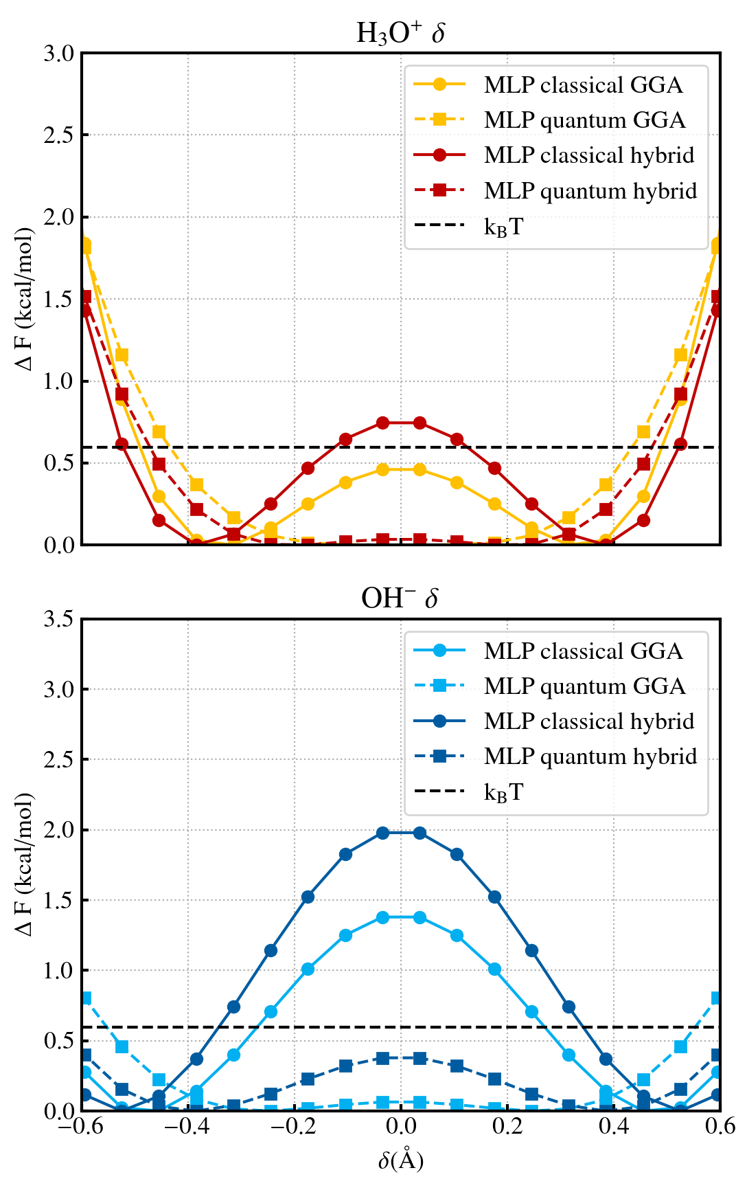
Figure 7: Free energy, $\Delta$F, along the proton sharing coordinate $\delta$, for the acid (top) and base (bottom) obtained from MLP simulations at 300 K. The dashed line shows $k_{\mathrm{B}}T$ at 300 K.

Comparing the simulated diffusion coefficients to their experimental values obtained from conductivity data at 301 K for H₃O⁺ (9.4 $\times$ 10^-9 m²/s) and OH^- (5.2 $\times$ 10^-9 m²/s) Sluyters and Sluyters-Rehbach (2010), both the classical GGA and quantum hybrid H₃O⁺ simulations (8.0 $\times$ 10^-9 and 10.9 $\times$ 10^-9 m²/s) most closely reproduce the experimental H₃O⁺ diffusion coefficient, while the classical GGA OH^- simulations (4.9 $\times$ 10^-9 m²/s) most closely reproduce the experimental OH^- diffusion coefficient. The strong performance of the classical GGA trajectories can likely be attributed to the cancellation of error between proton delocalization due to overestimated hydrogen bond strengths and proton localization due to the classical treatment of nuclei. Quantum hybrid trajectories also perform relatively well because they incorporate NQEs, and the revPBE0-D3 functional less severely overestimates hydrogen bond strengths. Notably, when NQEs are included for both the GGA and hybrid functionals, the ratios of the excess proton diffusion coefficient to that of the hydroxide ion diffusion coefficient, 1.1 and 1.2 respectively, are lower than the experimentally observed value of 1.8, and are in worse agreement for this property than when the nuclei are treated classically (1.6 and 2.2 for the GGA and hybrid simulations respectively). This arises from the much more pronounced NQEs on the hydroxide diffusion coefficient than the excess proton, with a factor of 2.5 and 2.6 increase for the GGA and hybrid upon going from classical to quantum for the hydroxide ion but only 1.7 and 1.4 for the excess proton.

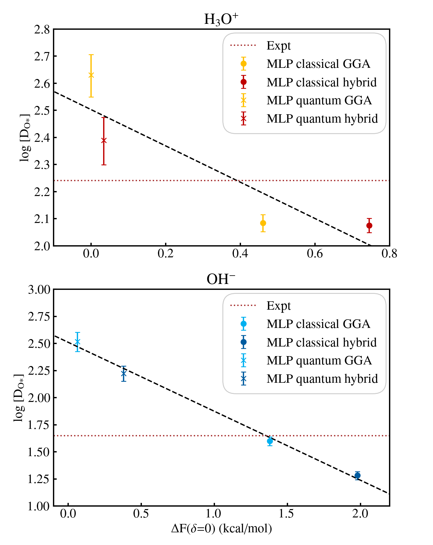
Figure 8: Diffusion coefficients as a function of the proton sharing coordinate free energy barrier, $\Delta$ F $(\delta=0)$, for the excess proton (top) and hydroxide ion (bottom) obtained from our MLP simulations. Our data show a much stronger correlation for the base than for the acid.

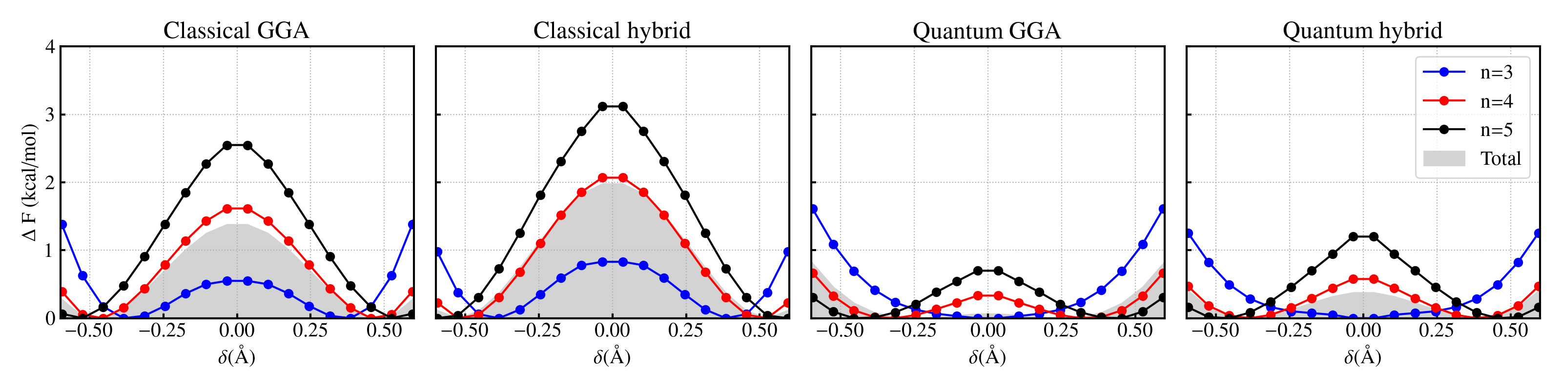
Figure 9: Values for the free energy barrier along the proton sharing coordinate $\delta$ at 3, 4, and 5 accepted hydrogen bonds at the OH^- for all MLP trajectories. The $\Delta$F($\delta$) for all OH^- is also shown for each trajectory.

To further analyze trends in the hydroxide ion diffusion coefficient and the impact of NQEs, we now explore the relationship between the rate of diffusion of OH^- and the proton transfer free energy barrier, $\Delta F(\delta=0)$. Previous studies have suggested that OH^- predominantly exists in an inert hypercoordinated state where it accepts four hydrogen bonds and transiently donates one Tuckerman, Chandra, and Marx (2006); Chen et al. (2018). In this picture, proton transfer occurs after thermal fluctuations break one of the accepted hydrogen bonds, converting the inert hypercoordinated OH^- to a tetrahedral active state that accepts three hydrogen bonds and donates one. The OH^- is then ready to accept a proton from a neighboring molecule because it has assumed the tetrahedral geometry typical of neutral water molecules, a concept known as presolvation Tuckerman, Chandra, and Marx (2006). The hypercoordination of OH^- is the primary reason why the mechanism of transport of OH^- cannot simply be inferred from that of H₃O⁺, which typically donates three hydrogen bonds.

Our MLP simulations support the hypercoordination picture, with the less active state where OH^- accepts four hydrogen bonds making up the majority of frames for all of the trajectories, i.e. 63%, 56%, 50%, and 58% of all frames in the classical GGA, classical hybrid, quantum GGA, and quantum hybrid trajectories respectively. In all cases, the percentage of all proton hops where the recipient is a triply-coordinated OH^- is higher than the percentage of all OH^- configurations that are triply coordinated. In particular, for the classical simulations, 51% and 44% (GGA and hybrid) of all proton hops are to triply-coordinated OH^- while only 13% and 7% of all OH^- configurations are triply coordinated. A similar trend is observed for the quantum simulations, where 62.6% and 51.5% (GGA and hybrid) of all proton hops are to triply-coordinated OH^-, while only 41% and 20% of all OH^- configurations are triply coordinated. Further analysis shows that the hydroxide ion diffusion coefficient is positively correlated with the percentage of proton hops to a triply-coordinated OH^-. Additionally, there is a clear inverse correlation between the free energy barrier along the proton sharing coordinate and the OH^- coordination number. Figure 9 shows the computed free energy barriers for OH^- at different numbers of accepted hydrogen bonds (n={3,4,5}). OH^- ions that accept three hydrogen bonds have the lowest $\Delta$F across all trajectories, further suggesting that the n=3 state is indeed the active proton transfer state, in line with previous studiesTuckerman, Chandra, and Marx (2006); Chen et al. (2018).

We observe that the impact of NQEs on the proton transfer barrier is two-fold: the direct effect of lowering the barrier along the proton sharing coordinate and the indirect effect of shifting the distribution of hypercoordinated states towards the more favorable states for proton transfer to occur. Specifically, in Fig. 9 one sees that $\Delta F(\delta=0)$ is lower for the quantum trajectories for any given value of the OH^- coordination (e.g. n=3, n=4, etc.). This direct effect lowers the barrier by as much as 1.92 kcal/mol in the n=5 state and by 0.83 kcal/mol in the n=3 state. Conversely, NQEs provide an indirect effect by markedly increasing the incidence of triply coordinated OH^- configurations: 12.6%, and 6.7% of all frames for classical GGA and hybrid trajectories respectively, compared to 41% and 20% of all frames in the quantum GGA and hybrid trajectories respectively.

VI Conclusion

We have presented two MLPs—trained on revPBE-D3 (GGA) and revPBE0-D3 (hybrid) AIMD energies and forces—that simultaneously capture the properties of excess protons and hydroxide ions in water. To test the validity of our MLPs, we benchmarked the GGA MLP against independent GGA AIMD trajectories of an excess proton in water and a hydroxide ion in water. Overall, the GGA MLP faithfully reproduced several of the most challenging ab initio properties relevant to proton defects, namely the H^∗ and O^∗ VDOS, the free energy barrier along $\delta$, and the RDFs (H^∗–H, O^∗–H, O^∗–O).

Our hybrid and GGA MLPs were then used to perform multi-nanosecond classical and TRPMD trajectories of the excess proton and hydroxide ion, enabling us to obtain diffusion properties of the proton defects with minimal statistical noise. By analyzing these simulations, we elucidated how the choice of DFT functional (GGA vs hybrid) and nuclear representation (classical vs quantum) affects the rate of both molecular and proton defect diffusion. By comparing the proton defect diffusion coefficient to the free energy barrier along the proton sharing coordinate ($\delta$), we showed that a higher free energy barrier is correlated with a low rate of proton transfer, although the correlation is stronger for the hydroxide ion than for the excess proton. Additionally, by calculating the free energy barrier along $\delta$ for different coordination states of the OH^- ion, we showed that our data agree with prior studies Tuckerman, Chandra, and Marx (2006); Chen et al. (2018) that posit a predominantly inert quadruply hydrogen-bonded OH^- that occasionally undergoes thermal fluctuations to lose one of its accepted hydrogen bonds in order to enter a tetrahedral state that is conducive to proton transfer.

The MLP models we introduce here provide a means to run multi-nanosecond molecular dynamics simulations of proton defects in water at DFT-level accuracy and low computational cost, thus enabling one to study rare events with unprecedented statistical accuracy. In addition, the training set constructed in this work provides a starting point for training MLPs that are able to treat both proton and hydroxide defects, and hence processes such as autoionization, at higher levels of electronic structure theory or for more diverse chemical environments. This lays the groundwork for improving our understanding of the finer details of the proton transfer mechanism in water, as well as the mechanics of autoionization and proton-hydroxide recombination events.

Data Availability

The data that supports the findings of this study are available within the article and its supplementary material.

VII References

References

- Peighambardoust, Rowshanzamir, and Amjadi (2010) S. Peighambardoust, S. Rowshanzamir, and M. Amjadi, International Journal of Hydrogen Energy 35, 9349 (2010).
- DeCoursey (2018) T. E. DeCoursey, Journal of The Royal Society Interface 15, 20180108 (2018).
- Marx (2006) D. Marx, ChemPhysChem 7, 1848 (2006).
- Hassanali et al. (2013) A. Hassanali, F. Giberti, J. Cuny, T. D. Kühne, and M. Parrinello, Proceedings of the National Academy of Sciences 110, 13723 (2013).
- Halle and Karlström (1983a) B. Halle and G. Karlström, J. Chem. Soc., Faraday Trans. 2 79, 1047 (1983a).
- Halle and Karlström (1983b) B. Halle and G. Karlström, J. Chem. Soc., Faraday Trans. 2 79, 1031 (1983b).
- Weingärtner and Chatzidimttriou-Dreismann (1990) H. Weingärtner and C. A. Chatzidimttriou-Dreismann, Nature 346, 548 (1990).
- Sluyters and Sluyters-Rehbach (2010) J. H. Sluyters and M. Sluyters-Rehbach, The Journal of Physical Chemistry B 114, 15582 (2010).
- Tuckerman et al. (1995a) M. Tuckerman, K. Laasonen, M. Sprik, and M. Parrinello, The Journal of Physical Chemistry 99, 5749 (1995a).
- Tuckerman et al. (1995b) M. Tuckerman, K. Laasonen, M. Sprik, and M. Parrinello, The Journal of Chemical Physics 103, 150 (1995b).
- Agmon (1995) N. Agmon, Chemical Physics Letters 244, 456 (1995).
- Marx et al. (1999) D. Marx, M. E. Tuckerman, J. Hutter, and M. Parrinello, Nature 397, 601 (1999).
- Marx, Tuckerman, and Parrinello (2000) D. Marx, M. E. Tuckerman, and M. Parrinello, Journal of Physics: Condensed Matter 12, A153 (2000).
- Vuilleumier and Borgis (1999) R. Vuilleumier and D. Borgis, The Journal of Chemical Physics 111, 4251 (1999).
- Day, Schmitt, and Voth (2000) T. J. F. Day, U. W. Schmitt, and G. A. Voth, Journal of the American Chemical Society 122, 12027 (2000).
- Tuckerman, Marx, and Parrinello (2002) M. E. Tuckerman, D. Marx, and M. Parrinello, Nature 417, 925 (2002).
- Agmon et al. (2016) N. Agmon, H. J. Bakker, R. K. Campen, R. H. Henchman, P. Pohl, S. Roke, M. Thämer, and A. Hassanali, Chemical Reviews 116, 7642 (2016).
- Hückel (1928) E. Hückel, Zeitschrift für Elektrochemie und angewandte physikalische Chemie 34, 546 (1928).
- Eigen (1964) M. Eigen, Angewandte Chemie International Edition in English 3, 1 (1964).
- Stillinger (1978) F. Stillinger, Theoretical Chemistry Advances and Perspectives, edited by H. Eyring (Academic, New York, 1978) pp. 177–234.
- Zatsepina (1972) G. Zatsepina, Journal of Structural Chemistry 12, 894 (1972).
- Schiöberg and Zundel (1973) D. Schiöberg and G. Zundel, Journal of the Chemical Society, Faraday Transactions 2: Molecular and Chemical Physics 69, 771 (1973).
- Librovich, Sakun, and Sokolov (1979) N. Librovich, V. Sakun, and N. Sokolov, Chemical Physics 39, 351 (1979).
- Khoshtariya and Berdzenishvili (1992) D. E. Khoshtariya and N. O. Berdzenishvili, Chemical physics letters 196, 607 (1992).
- Agmon (2000) N. Agmon, Chemical Physics Letters 319, 247 (2000).
- Napoli, Marsalek, and Markland (2018) J. A. Napoli, O. Marsalek, and T. E. Markland, The Journal of Chemical Physics 148, 222833 (2018).
- Cao and Voth (1994) J. Cao and G. A. Voth, The Journal of Chemical Physics 100, 5106 (1994).
- Jang and Voth (1999) S. Jang and G. A. Voth, The Journal of Chemical Physics 111, 2371 (1999).
- Craig and Manolopoulos (2004) I. R. Craig and D. E. Manolopoulos, The Journal of Chemical Physics 121, 3368 (2004).
- Habershon et al. (2013) S. Habershon, D. E. Manolopoulos, T. E. Markland, and T. F. Miller, Annual Review of Physical Chemistry 64, 387 (2013).
- Ceriotti et al. (2016) M. Ceriotti, W. Fang, P. G. Kusalik, R. H. McKenzie, A. Michaelides, M. A. Morales, and T. E. Markland, Chemical Reviews 116, 7529 (2016).
- Markland and Ceriotti (2018) T. E. Markland and M. Ceriotti, Nature Reviews Chemistry 2 (2018), 10.1038/s41570-017-0109.
- Tuckerman, Berne, and Martyna (1992) M. Tuckerman, B. J. Berne, and G. J. Martyna, The Journal of Chemical Physics 97, 1990 (1992).
- Markland and Manolopoulos (2008a) T. E. Markland and D. E. Manolopoulos, The Journal of Chemical Physics 129, 024105 (2008a).
- Markland and Manolopoulos (2008b) T. E. Markland and D. E. Manolopoulos, Chemical Physics Letters 464, 256 (2008b).
- Fanourgakis, Markland, and Manolopoulos (2009) G. S. Fanourgakis, T. E. Markland, and D. E. Manolopoulos, The Journal of Chemical Physics 131, 094102 (2009).
- Marsalek and Markland (2016) O. Marsalek and T. E. Markland, The Journal of Chemical Physics 144, 054112 (2016).
- Kapil, VandeVondele, and Ceriotti (2016) V. Kapil, J. VandeVondele, and M. Ceriotti, The Journal of Chemical Physics 144, 054111 (2016).
- Marsalek and Markland (2017) O. Marsalek and T. E. Markland, The Journal of Physical Chemistry Letters 8, 1545 (2017).
- Gasparotto, Hassanali, and Ceriotti (2016) P. Gasparotto, A. A. Hassanali, and M. Ceriotti, Journal of Chemical Theory and Computation 12, 1953 (2016).
- Cheng et al. (2019) B. Cheng, E. A. Engel, J. Behler, C. Dellago, and M. Ceriotti, Proceedings of the National Academy of Sciences 116, 1110 (2019).
- Behler and Parrinello (2007) J. Behler and M. Parrinello, Phys. Rev. Lett. 98, 146401 (2007).
- Behler (2011) J. Behler, The Journal of Chemical Physics 134, 074106 (2011).
- Behler (2014) J. Behler, Journal of Physics: Condensed Matter 26, 183001 (2014).
- Natarajan, Morawietz, and Behler (2015) S. K. Natarajan, T. Morawietz, and J. Behler, Physical Chemistry Chemical Physics 17, 8356 (2015).
- Schran, Behler, and Marx (2019) C. Schran, J. Behler, and D. Marx, Journal of Chemical Theory and Computation 16, 88 (2019).
- Hellström and Behler (2016) M. Hellström and J. Behler, The Journal of Physical Chemistry Letters 7, 3302 (2016).
- Hellström, Ceriotti, and Behler (2018) M. Hellström, M. Ceriotti, and J. Behler, The Journal of Physical Chemistry B 122, 10158 (2018).
- Morawietz et al. (2018) T. Morawietz, O. Marsalek, S. R. Pattenaude, L. M. Streacker, D. Ben-Amotz, and T. E. Markland, The Journal of Physical Chemistry Letters 9, 851 (2018).
- Perdew, Burke, and Ernzerhof (1996) J. P. Perdew, K. Burke, and M. Ernzerhof, Physical Review Letters 77, 3865 (1996).
- Zhang and Yang (1998) Y. Zhang and W. Yang, Physical Review Letters 80, 890 (1998).
- Adamo and Barone (1999) C. Adamo and V. Barone, The Journal of Chemical Physics 110, 6158 (1999).
- Goerigk and Grimme (2011) L. Goerigk and S. Grimme, Physical Chemistry Chemical Physics 13, 6670 (2011).
- Grimme et al. (2010) S. Grimme, J. Antony, S. Ehrlich, and H. Krieg, The Journal of Chemical Physics 132, 154104 (2010).
- VandeVondele et al. (2005) J. VandeVondele, M. Krack, F. Mohamed, M. Parrinello, T. Chassaing, and J. Hutter, Computer Physics Communications 167, 103 (2005).
- Kühne et al. (2020) T. D. Kühne, M. Iannuzzi, M. D. Ben, V. V. Rybkin, P. Seewald, F. Stein, T. Laino, R. Z. Khaliullin, O. Schütt, F. Schiffmann, D. Golze, J. Wilhelm, S. Chulkov, M. H. Bani-Hashemian, V. Weber, U. Borštnik, M. Taillefumier, A. S. Jakobovits, A. Lazzaro, H. Pabst, T. Müller, R. Schade, M. Guidon, S. Andermatt, N. Holmberg, G. K. Schenter, A. Hehn, A. Bussy, F. Belleflamme, G. Tabacchi, A. Glöß, M. Lass, I. Bethune, C. J. Mundy, C. Plessl, M. Watkins, J. VandeVondele, M. Krack, and J. Hutter, The Journal of Chemical Physics 152, 194103 (2020).
- Goedecker, Teter, and Hutter (1996) S. Goedecker, M. Teter, and J. Hutter, Physical Review B 54, 1703 (1996).
- Lippert, Hutter, and Parrinello (1997) G. Lippert, J. Hutter, and M. Parrinello, Molecular Physics 92, 477 (1997).
- VandeVondele and Hutter (2007) J. VandeVondele and J. Hutter, The Journal of Chemical Physics 127, 114105 (2007).
- Behler (2016) J. Behler, “Runner – a software package for constructing high-dimensional neural network potentials,” (2007-2016).
- Singraber et al. (2021) A. Singraber, Mpbircher, S. Reeve, D. W. Swenson, J. Lauret, and Philippedavid, “Compphysvienna/n2p2: Version 2.1.4,” (2021).
- Morawietz et al. (2016) T. Morawietz, A. Singraber, C. Dellago, and J. Behler, Proceedings of the National Academy of Sciences 113, 8368 (2016).
- Thompson et al. (2022) A. P. Thompson, H. M. Aktulga, R. Berger, D. S. Bolintineanu, W. M. Brown, P. S. Crozier, P. J. in ’t Veld, A. Kohlmeyer, S. G. Moore, T. D. Nguyen, R. Shan, M. J. Stevens, J. Tranchida, C. Trott, and S. J. Plimpton, Comp. Phys. Comm. 271, 108171 (2022).
- Singraber, Behler, and Dellago (2019) A. Singraber, J. Behler, and C. Dellago, Journal of Chemical Theory and Computation 15, 1827 (2019).
- Bussi, Donadio, and Parrinello (2007) G. Bussi, D. Donadio, and M. Parrinello, The Journal of Chemical Physics 126, 014101 (2007).
- Ceriotti, More, and Manolopoulos (2014) M. Ceriotti, J. More, and D. E. Manolopoulos, Computer Physics Communications 185, 1019 (2014).
- Kapil et al. (2019) V. Kapil, M. Rossi, O. Marsalek, R. Petraglia, Y. Litman, T. Spura, B. Cheng, A. Cuzzocrea, R. H. Meißner, D. M. Wilkins, B. A. Helfrecht, P. Juda, S. P. Bienvenue, W. Fang, J. Kessler, I. Poltavsky, S. Vandenbrande, J. Wieme, C. Corminboeuf, T. D. Kühne, D. E. Manolopoulos, T. E. Markland, J. O. Richardson, A. Tkatchenko, G. A. Tribello, V. V. Speybroeck, and M. Ceriotti, Computer Physics Communications 236, 214 (2019).
- Rossi, Ceriotti, and Manolopoulos (2014) M. Rossi, M. Ceriotti, and D. E. Manolopoulos, The Journal of Chemical Physics 140, 234116 (2014).
- Ceriotti et al. (2010) M. Ceriotti, M. Parrinello, T. E. Markland, and D. E. Manolopoulos, The Journal of Chemical Physics 133, 124104 (2010).
- VandeVondele and Hutter (2003) J. VandeVondele and J. Hutter, The Journal of Chemical Physics 118, 4365 (2003).
- Kolafa (2003) J. Kolafa, Journal of Computational Chemistry 25, 335 (2003).
- Kühne et al. (2007) T. D. Kühne, M. Krack, F. R. Mohamed, and M. Parrinello, Physical Review Letters 98 (2007), 10.1103/physrevlett.98.066401.
- Luzar and Chandler (1996) A. Luzar and D. Chandler, Physical Review Letters 76, 928 (1996).
- Yeh and Hummer (2004) I.-C. Yeh and G. Hummer, The Journal of Physical Chemistry B 108, 15873 (2004).
- Fournier et al. (2018) J. A. Fournier, W. B. Carpenter, N. H. C. Lewis, and A. Tokmakoff, Nature Chemistry 10, 932 (2018).
- Headrick, Bopp, and Johnson (2004) J. M. Headrick, J. C. Bopp, and M. A. Johnson, The Journal of Chemical Physics 121, 11523 (2004).
- Headrick et al. (2005) J. M. Headrick, E. G. Diken, R. S. Walters, N. I. Hammer, R. A. Christie, J. Cui, E. M. Myshakin, M. A. Duncan, M. A. Johnson, and K. D. Jordan, Science 308, 1765 (2005).
- Asmis et al. (2003) K. R. Asmis, N. L. Pivonka, G. Santambrogio, M. Brümmer, C. Kaposta, D. M. Neumark, and L. Wöste, Science 299, 1375 (2003).
- Roberts et al. (2009) S. T. Roberts, P. B. Petersen, K. Ramasesha, A. Tokmakoff, I. S. Ufimtsev, and T. J. Martinez, Proceedings of the National Academy of Sciences 106, 15154 (2009).
- Holz, Heil, and Sacco (2000) M. Holz, S. R. Heil, and A. Sacco, Physical Chemistry Chemical Physics 2, 4740 (2000).
- Gillan, Alfè, and Michaelides (2016) M. J. Gillan, D. Alfè, and A. Michaelides, The Journal of Chemical Physics 144, 130901 (2016).
- Habershon, Markland, and Manolopoulos (2009) S. Habershon, T. E. Markland, and D. E. Manolopoulos, The Journal of Chemical Physics 131, 024501 (2009).
- Chen et al. (2003) B. Chen, I. Ivanov, M. L. Klein, and M. Parrinello, Physical Review Letters 91 (2003), 10.1103/physrevlett.91.215503.
- Markland and Berne (2012) T. E. Markland and B. J. Berne, Proceedings of the National Academy of Sciences 109, 7988 (2012).
- Li, Walker, and Michaelides (2011) X.-Z. Li, B. Walker, and A. Michaelides, Proceedings of the National Academy of Sciences 108, 6369 (2011).
- McKenzie (2012) R. H. McKenzie, Chemical Physics Letters 535, 196 (2012).
- McKenzie et al. (2014) R. H. McKenzie, C. Bekker, B. Athokpam, and S. G. Ramesh, The Journal of Chemical Physics 140, 174508 (2014).
- Guidon et al. (2008) M. Guidon, F. Schiffmann, J. Hutter, and J. VandeVondele, The Journal of Chemical Physics 128, 214104 (2008).
- Zhang et al. (2011) C. Zhang, D. Donadio, F. Gygi, and G. Galli, Journal of Chemical Theory and Computation 7, 1443 (2011).
- DiStasio et al. (2014) R. A. DiStasio, B. Santra, Z. Li, X. Wu, and R. Car, The Journal of Chemical Physics 141, 084502 (2014).
- Miceli, de Gironcoli, and Pasquarello (2015) G. Miceli, S. de Gironcoli, and A. Pasquarello, The Journal of Chemical Physics 142, 034501 (2015).
- Chen et al. (2023) M. S. Chen, J. Lee, H.-Z. Ye, T. C. Berkelbach, D. R. Reichman, and T. E. Markland, Journal of Chemical Theory and Computation (2023), 10.1021/acs.jctc.2c01203.
- Babin, Leforestier, and Paesani (2013) V. Babin, C. Leforestier, and F. Paesani, Journal of Chemical Theory and Computation 9, 5395 (2013).
- Babin, Medders, and Paesani (2014) V. Babin, G. R. Medders, and F. Paesani, Journal of Chemical Theory and Computation 10, 1599 (2014).
- Medders, Babin, and Paesani (2014) G. R. Medders, V. Babin, and F. Paesani, Journal of Chemical Theory and Computation 10, 2906 (2014).
- Reddy et al. (2016) S. K. Reddy, S. C. Straight, P. Bajaj, C. H. Pham, M. Riera, D. R. Moberg, M. A. Morales, C. Knight, A. W. Götz, and F. Paesani, The Journal of Chemical Physics 145, 194504 (2016).
- Yu et al. (2022) Q. Yu, C. Qu, P. L. Houston, R. Conte, A. Nandi, and J. M. Bowman, The Journal of Physical Chemistry Letters 13, 5068 (2022).
- Tuckerman, Chandra, and Marx (2006) M. E. Tuckerman, A. Chandra, and D. Marx, Accounts of Chemical Research 39, 151 (2006).
- Chen et al. (2018) M. Chen, L. Zheng, B. Santra, H.-Y. Ko, R. A. D. Jr, M. L. Klein, R. Car, and X. Wu, Nature Chemistry 10, 413 (2018).