Vibrational spectroscopies in liquid water: on temperature and coordination effects in Raman and infrared spectroscopies

Abstract

Water is an ubiquitous liquid that has several exotic and anomalous properties. Despite its apparent simple chemical formula, its capability of forming a dynamic network of hydrogen bonds leads to a rich variety of physics. Here we study the vibrations of water using molecular dynamics simulations, mainly concentrating on the Raman and infrared spectroscopic signatures. We investigate the consequences of the temperature on the vibrational frequencies, and we enter the details of the hydrogen bonding coordination by using restrained simulations in order to gain quantitative insight on the dependence of the frequencies on the neighbouring molecules. Further we consider the differences due to the different methods of solving the electronic structure to evaluate the forces on the ions, and report results on the angular correlations, isotopic mixtures HOD in H₂O/D₂O and and the dielectric constants in water.

Key words: water, computer simulations, vibrational spectroscopy, molecular dynamics, density functional theory, hydrogen bonds

Abstract

Âîäà є íàéïîøèðåíiøîþ ðiäèíîþ, ùî âîëîäiє áàãàòüìà åêçîòèчíèìè òà àíîìàëüíèìè âëàñòèâîñòÿìè. Íåçâàæàþчè íà îчåâèäíó ïðîñòó õiìiчíó ôîðìóëó, ¿¿ çäàòíiñòü óòâîðþâàòè äèíàìiчíó ñiòêó âîäíåâèõ çâ’ÿçêiâ ïðèçâîäèòü äî âèíèêíåííÿ ðiçíîìàíiòíèõ ôiçèчíèõ åôåêòiâ. Äîñëiäæóþòüñÿ êîëèâàííÿ ó âîäi íà îñíîâi ìîëåêóëÿðíî¿ äèíàìiêè ç àêöåíòîì ïåðåâàæíî íà ñèãíàòóðàõ êîìáiíàöiéíèõ òà iíôðàчåðâîíèõ ñïåêòðiâ. Âèâчåíî âïëèâ òåìïåðàòóðè íà êîëèâíi ñïåêòðè; ââåäåíî äåòàëi êîîðäèíàöiéíèõ ñïiââiäíîøåíü ìiæ âîäíåâèìè çâ’ÿçêàìè íà îñíîâi ìîäåëþâàííÿ ç åíåðãåòèчíèìè îáìåæåííÿìè äëÿ îòðèìàííÿ êiëüêiñíî¿ iíôîðìàöi¿ ïðî çàëåæíiñòü чàñòîò ñóñiäíiõ ìîëåêóë. Òàêîæ ðîçãëÿíóòî âiäìiííîñòi, ùî âèíèêàþòü ïðè âèêîðèñòàííi ðiçíèõ ìåòîäiâ ðîçðàõóíêó åëåêòðîííî¿ ñòðóêòóðè äëÿ îáчèñëåííÿ ñèë, ùî äiþòü íà iîíè. Íàâåäåíî ðåçóëüòàòè äëÿ êóòîâèõ êîðåëÿöié, äëÿ içîòîïíèõ ñóìiøåé HOD â H₂O/D₂O òà äiåëåêòðèчíèõ ñòàëèõ âîäè.

Ключовi слова: âîäà, êîìï’þòåðíå ìîäåëþâàííÿ, êîëèâíà ñïåêòðîñêîïiÿ, ìîëåêóëÿðíà äèíàìiêà, ìåòîä ôóíêöiîíàëó ãóñòèíè, âîäíåâi çâ’ÿçêè

1 Introduction

The vibrational properties of liquid water are already well known — there is of course a plethora of literature on the topic, for a recent review please see for example [1]. The methods mostly used to characterise them are the infrared (IR) and Raman spectroscopies in the local frame, and inelastic neutron and X-ray scattering for the collective modes. The spectra consist of high-frequency region, that stems from the intramolecular O-H stretching motions, intramolecular H-O-H bending mode and the low-frequency modes plus possibly combination modes and overtones, that arise from the motion of the water molecules with respect to each other. The details of the vibrations change according to the instantaneous environment of the molecules, in particular, the hydrogen bond (HB) network, that forms as a “glue” between the molecules in the liquid. It is the influence of these HBs on the vibrational frequencies that we want to characterise in the present work.

An interesting temperature dependency of the signal in the O-H stretching bond region in (IR) and Raman vibrational spectroscopies is known: the intensity shifts to higher frequencies upon heating of the system. This can be understood in terms of the changing coordination in the HB network formed between the molecules: at low temperatures more HBs are present and thus the vibrational frequencies are lowered due to the attractive interactions along the O-H intramolecular bonds, causing the bond length to elongate and thus lower the frequency. At higher temperatures, many of the HBs are lost and the molecules approach the higher vibrational frequencies of a free water monomer. Thereby the vibrational frequencies at varying temperatures are indirectly functions of the intermolecular HB network, and thus the HB coordination of a given molecule.

The computation of IR and Raman spectra directly from the electronic structure in the condensed phase was developed along the appearance of “modern theory of polarization” [2]. It was soon applied to simulation of the IR spectra of water by Parrinello and co-workers [3], and soon the implementation of Raman spectra followed together with an application in ice [4].

Here we present atomistic molecular dynamics (MD) simulations of the temperature dependency of the Raman and IR signals. The first studies of Raman spectra directly from the electronic structure appeared some time ago [5]. Furthermore, we evaluate the Raman signal from the MD trajectories recently simulated by Del Ben and co-workers using the MP2 ab initio electronic structure methods to evaluate the interactions between the water molecules [6]. In order to fully characterize the underlying HB network, we first provide an analysis of the structural and dynamical properties of the samples. We then proceed to analysing the simulated spectra, and divide the changes detected to their origins in the HB network.

We further note that nowadays it would be more fashionable to run the simulations performed here using the potentials and required quantities such as the polarizability developed via machine learning [7] rather than running them with the explicitly resolved electronic structure at each time step. This approach could be used to reduce the errors due to the needy sampling of the statistics, nuclear quantum effects, and one is able to apply more accurate methods in solving the electronic structure and so on.

The present work is organized as follows: in section 2 we present the methods of simulation and analysis and the notation, in section 3 we present the results obtained from our analysis and in section 4 we put our results into perspective of what is already known about the vibrational spectroscopy of water and what we have learnt here.

We already humbly apologize here for the omissions that we cannot cover all the vast, sometimes even contradictory, literature and models and results present in the literature from about a century of scientific discoveries.

2 Methods

We have performed density functional theory-based molecular dynamics (DFTb-MD), where the ions are moved according to the Newtonian equations of motion according to the forces derived from the density functional theory (DFT) [8]. The nuclei, in particular, the protons — with the neutron when simulating with deuterium — in the hydrogen atoms, are treated as point particles and we rely on the Born-Oppenheimer approximation. Thus, the dynamics is performed using classical dynamics, leading to non-quantized dynamics and, therefore, we should expect to obtain exactly the same results as in the results from the experiments, added to the other approximations that we are employing.

2.1 Systems

Our samples consisted of 128 water molecules in a periodically repeated cell; in the MP2 simulations, 64 water molecules had been used instead [6]. The different systems simulated are listed in table 1. For computational simplicity we used the same, ambient experimental density in all the simulations. In the DFTb-MD simulations results on the angular correlations, isotopic lattice constant of isotropic mixtures was 15.7459 Å, corresponding to a density of 0.9808 g/cm³ of light or 1.0904 g/cm³ of deuterated water.

Table 1: Summary of the system parameters: targeted temperature ($T$), the resulting average intramolecular O-H bond length $d_{\mathrm{O-H}}$, average band gap, dipole moment $\mu_{\text{W}}$ and average polarizability $\overline{\alpha}$, diffusion constant $D_{\text{O}}$ of O evaluated via the Einstein (E) or Green-Kubo (GK) formalism. XC(traj) is the approach used in generating the trajectory and XC(pol) in calculating the band gap, dipole moment or polarizability.

	$T$	$d_{\mathrm{O-H}}$	gap	$\mu_{\text{W}}$	$\overline{\alpha}$	$D_{\mathrm{O}}^{\mathrm{E}}$	$D_{\mathrm{O}}^{\mathrm{GK}}$
Notation	[K]	[Å]	[eV]	[D]	[Å3]	[Å2/ps]
XC: BLYP+D3 128 H2O/D2O
D2O–$T=25$℃	298.15	0.992	4.39	3.03	1.771	0.08	0.10
D2O–$T=50$℃	323.15	0.990	4.29	2.96	1.767	0.21	0.18
D2O–$T=75$℃	348.15	0.990	4.18	2.93	1.765	0.29	0.23
D2O–$T=100$℃	373.15	0.989	4.12	2.89	1.761	0.40	0.37
D2O–$T=125$℃	398.15	0.988	4.02	2.85	1.760	0.51	0.59
H2O–$T=50$℃	323.15	0.992	4.30	2.99	1.769	0.17	0.21
H2O@D2O–$T=50$℃	323.15	0.992/0.991	4.31	3.03	1.769	0.07/0.08	0.14/0.13
D2O@H2O–$T=50$℃	323.15	0.991/0.991	4.31	3.05	1.767	0.39/0.17	0.07/0.13
HOD@D2O–$T=50$℃	323.15	0.991/0.991/0.992	4.32	2.98	1.774	0.28/0.17	0.11/0.15
HOD@H2O–$T=50$℃	323.15	0.992/0.991/0.990	4.28	2.99	1.769	0.16/0.22	0.08/0.14
XC: revPBE+D3 128 D2O
D2O–$T=25$℃	298.15	0.986	4.60	2.94	1.726	0.15	0.13
D2O–$T=50$℃	323.15	0.986	4.41	2.88	1.722	0.26	0.22
D2O–$T=75$℃	348.15	0.985	4.34	2.85	1.716	0.35	0.41
XC(traj): vdW-DF-rPW86/XC(pol): BLYP 128 H2O
H2O–vdW-DF/BLYP	323.15	0.984	4.00	2.80	1.751	0.34	0.37
XC(traj): MP2/XC(pol): BLYP 64 H2O
MP2/BLYP	298.15	0.978	4.67	3.02	1.667	0.07	0.08
XC(traj): MP2/XC(pol): PBE 64 H2O
MP2/PBE	298.15	0.978	4.67		1.685

We ran most of the simulations on the deuterated water, in order to reduce the error due to the employment of the classical equations of motion without quantum nuclear effects on the nuclei, and at somewhat elevated temperature of 50℃, since it is known that some of the methods used lead to samples that are near the amorphous liquids close to the real melting point of the liquid, in particular the BLYP+D3 that is described below.

2.2 Computational details

We have carried out DFTb-MD calculations using a hybrid Gaussian plane-wave (GPW) method [9] as implemented in the QuickStep module [10] in the CP2K suite of programs [11]. This approach combines a Gaussian basis set for the wave functions with an auxiliary plane wave basis set for the density. We chose a triple-zeta valence doubly polarised (TZV2P) basis set since it has been shown to provide a good compromise between accuracy and computational cost [12]. The cut-off for the electronic density was set to 400 Ry, in conjunction with the use of a smoothing method (NN50) for the exchange-correlation contribution [10]. The smoothing method has been found essential in our recent study of water [13] to obtain converged forces.

The action of core electrons on the (pseudo) valence orbitals was replaced by the Goedecker-Teter-Hutter (GTH) norm-conserving pseudo-potentials [14, 15]. The BLYP exchange-correlation (XC) functional [16, 17] of type generalised gradient approximation (GGA) has been used together with semi-empirical additional three-body potential [18] to account for the dispersion interactions missing in the GGA [19]. Improvement in the simulation of neat water was already shown in our previous study [13]. Since at the time of the evaluations of the polarizabilities, dipole moments and band gaps, the usage of MP2 and vdW-DF was not available or would have been prohibitively expensive computational task, we used either BLYP or the alternative GGA, Perdew-Burke-Ernzerhof (PBE) [20], to evaluate the electronic structure; the approximation of XC used is indicated as “XC(traj)” in table reftable:systems. Further, we simulated water using an explicit van der Waals-density functional; we applied the original vdW-DF [21] otherwise but the revised Perdew-Wang-86 (rPW86) approximation [22] in the exchange part, as was done also in the vdW-DF2 functional [23].

Born-Oppenheimer molecular dynamics simulations were carried out in the canonical, or the NVT ensemble with a Nosé-Hoover thermostat chain and a time step of 0.5 fs. Trajectories were run for at least 50 ps, the light water simulation H₂O–BLYP+D3 for over 150 ps. The properties were analyzed after an equilibration section of 10 ps. We remind the Reader here that the nuclear quantum effects have not been treated in the present study.

We characterize the HB network around a molecule by its HB coordination $C_{\mathrm{HB}}$, and we use the notation A_lD_nm when the central molecule accepts $l$ HBs and donates $n$ and $m$ HBs from the two hydrogen atoms on it. By symmetry, A_lD_nm corresponds to A_lD_mn.

In order to observe a stable coordination of the HBs on a single molecule, we constrained the local hydrogen bonding using restraints on collective variables on the coordination number of the form

$$C_{\mathrm{L}_{1},\mathrm{L}_{2}}=\frac{1}{\mathrm{N}_{\mathrm{L}_{1}}}\sum_{j=1}^{\mathrm{N}_{\mathrm{L}_{1}}}\Bigl{\{}\sum_{i=1}^{\mathrm{N}_{\mathrm{L}_{2}}}\frac{1-\left(r_{ij}/r_{0}\right)^{n}}{1-\left(r_{ij}/r_{0}\right)^{m}}\Bigr{\}},$$

where $\mathrm{L}_{2}$ is one of the two hydrogens or the oxygen atom on the central, constrained molecule and $\mathrm{L}_{1}$ is either any oxygen or hydrogen in the sample, correspondingly. We used a harmonic potential between the target value (number of hydrogens around a central oxygen or vice versa) and $C_{\mathrm{L}_{1},\mathrm{L}_{2}}$. The trajectory “A₂D₁₁s” is like the “A₂D₁₁” but the radius $r_{0}$ is smaller, forcing stronger the HBs; thus, “s” for “strict”. In “A₃D_nms” only the oxygen is constrained whereas the hydrogens are not restrained to form or to avoid HBs. We are aware that we only constrain the distance between the hydrogen and oxygen atoms, and there is no enforcement of a suitable directionality in the O-H$\cdots$O angle. Moreover, due to the relatively large radii used, this scheme does not necessarily lead to a definite hydrogen bond or the hindering of one because we do not wish to affect the vibrational modes strictly by forcing caging. Rather the absolute values and shifts should be regarded as trends.

2.3 Methods of analysis

There was used a geometrical definition of an HB, that was formed between two molecules when the O$\cdots$O distance is at most 3.5 Å and the H$-$O$\cdots$O angle is smaller than 30^∘.

The vibrational modes were analyzed by localizing them on the central, restrained molecule using the effective normal mode analysis (ENMA) method [24].

The evaluation of the polarizability [25] and the dipole moment was done using the correponding implementations in the CP2K suite.

The dielectric constants were calculated using the formulae

$$\frac{\varepsilon_{\infty}-1}{\varepsilon_{\infty}+2}=\frac{4\piup\alpha}{3\Omega},$$

$$\varepsilon=\varepsilon_{\infty}+\frac{\left\langle{}M^{2}\right\rangle-\left\langle{}M\right\rangle^{2}}{3\varepsilon_{0}\,k_{\mathrm{B}}T\,\Omega}\ ,$$

where $\alpha$ is the polarizability, $\Omega$ is the volume of the super cell and $M$ is the total dipole moment. We estimate the latter from the Berry phase of the dipole operator.

The frequencies from the MP2 trajectories were scaled with a uniform factor 0.94, similar to [6], to allow an easier comparison with the other data. All the power, IR and Raman spectra were multiplied with the frequency in resemblance to incorporating, and as an ad hoc correction due to, the quantum nature of the nuclei.

3 Results and discussions

3.1 Structure and dynamics

We characterized the geometrical structure of the liquid samples via the average number of HBs and intramolecular O-H bond length $d_{\mathrm{O-H}}$, radial distribution functions (RDF) $g(r)$, the dynamics with the diffusion constants, and the electronic properties by the average electronic band gap, molecular dipole moment and polarizability; the results are shown in table 1 and figures 1 and S1 [here and below, prefix “S” refers to the Supporting Material (SM)].

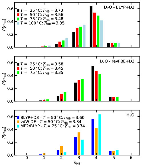
Figure 1: (Colour online) Distribution of $P(n_{\mathrm{HB}})$ and average $\bar{n}_{\mathrm{HB}}$ number of HBs per molecule.

Counter-intuitively, the average intramolecular bond length becomes slightly shorter upon increasing the temperature, but this is probably due to the concurrent reduction in the HBs. There are fewer HBs in the trajectory simulated with the vdW-DF, and the $d_{\mathrm{O-H}}$ is shorter than with BLYP+D3. MP2 yields the shortest O-H bond lengths, but the number of HBs is similar to the results with BLYP+D3 also at ambient temperature.

Except for $d_{\mathrm{O-H}}$ all the other studied quantities follow the expected trend upon an increase of the temperature: the number of HBs is reduced, even if the number of five-fold HB-coordinated molecules remains practically constant, the diffusion is enhanced, the electronic band gap is decreased due to larger geometrical fluctuations, the dipole moment decreases from the larger value found in ice and the polarizability is diminished.

In the RDF, the closest reminescense between the BLYP+D3 and the MP2 simulations is with the former simulated at $T=25$℃: the height of the peaks is very similar both in O-O and O-H correlations, but the position of the first maximum $r_{\mathrm{O-O}}^{\mathrm{max;1}}$ in $g_{\mathrm{O-O}}$ is at somewhat smaller radius in the MP2 results. This comparison is, however, somewhat blurred by the densities used: in the MP2 simulation the equilibrium density — about 2% larger than experimentally — had been used, whereas the BLYP+D3 samples are under pressure, the equilibrium density at $T=295$ K, $P=1$ bar being 1.066 g/cm³ [6]. The simulation applying the vdW-DF yields much less structured liquid than MP2 at $T=25$℃ or even BLYP+D3 at $T=100$℃, and $r_{\mathrm{O-O}}^{\mathrm{max;1}}$ is larger than even with BLYP+D3. Interestingly, data of the fifth-nearest-neighbour RDF, shown in figure S3, indicate that the fifth-closest O atom to the central O — as important indication of the liquid-like behaviour in water — does not get closer at the minimum encounters, but the relative magnitude at the maximum increases, as expected when the liquid becomes more diffusive upon higher temperature.

The electronic band gap gives a hint of the intra- and intermolecular arrangement, now that it was evaluated with the same treatment of the XC in all the computations of the Kohn-Sham eigenvalues. Therefore, it is interesting to notice that the value from the vdW-DF trajectory is clearly smaller, beyond the fluctuations (root-mean-square deviation $\approx$0.07 eV), than in the BLYP+D3 simulations at the same temperature, $T=50$℃.

We extract the values 1.964, 1.961, 1.960, 1.957, 1.956 for the dynamic dielectric constant with the BLYP+D3 approach in the D₂O at the different, increasing temperatures, 1.963 H₂O–$T=50$℃ with the BLYP+D3, 1.932, 1.929, 1.925 at the temperatures 25, 50 and 75℃ with the revPBE+D3, 1.950 with H₂O–vdW-DF/BLYP, and 1.949 and 1.963 in MP2/BLYP and MP2/PBE, respectively. On the dielectric constant $\varepsilon$ we extract a value of about 58, clearly but consistenly smaller than the value of $112\pm{}6$ obtained with the PBE approach and 64 water molecules at 350 K [26]. Details on the derivation of our value is given in the SM.

The diffusion constants $D_{\mathrm{O}}^{\mathrm{E}}$ and $D_{\mathrm{O}}^{\mathrm{GK}}$ have somewhat different values, but the differences are well within the statistical fluctuations, since much longer simulations should be performed to achieve a better convergence. The main effects, an increase in diffusion with the temperature in D₂O and respectively slower and faster diffusion with MP2 and vdW-DF than with BLYP+D3 in H₂O, are expected based on the relative magnitudes around the first minimum in the RDFs.

3.2 Dependence on temperature and XC

First we discuss the dependency of the Raman and infrared spectrum on the temperature, and various treatments of the electronic structure problem.

Before presenting the simulated spctra, we briefly discuss the power spectrum, that underlie the IR and Raman spectra. They are shown in figures S13 and S14, evaluated from the velocities of hydrogen or deuterium and the oxygen atoms in H₂O and D₂O. As the temperature is increased in D₂O, there are several systematic shifts along temperature: toward lower frequencies in regions around 300 and 650 cm^-1 and toward higher frequencies in the O-H stretching region around 2300 and 2600 cm^-1, where the latter effect is the most visible one and is seen clearly even in the power spectrum of O. The bending frequency is highly unaffected by the varying temperature, only via the height, which is set by normalizing the maximum of the whole spectrum and occurs in the O-H stretching region.

In H₂O, the vdW-DF- and MP2-treatments of the electronic structure lead to much narrower spectrum than BLYP+D3 in the O-H stretching region; we remind that the MP2 spectrum is multiplied by a constant whose value brings the maximum of the O-H stretching to the same region as BLYP+D3. Thereby, the maximum of the H-O-H stretching frequency is somewhat lower with MP2 than with BLYP+D3, but the spectra are very similar in region 300-1000 cm^-1. At around 280 cm^-1, vdW-DF has much lower intensity than BLYP+D3 or MP2, and at around 120 cm^-1 MP2 simulations yield a lower magnitude than BLYP+D3 or vdW-DF.

3.2.1 Raman spectra

The evaluated isotropic and anisotropic Raman spectra in D₂O and H₂O are presented in figures 2 together with experimental results [27, 28]. In the O-H stretching region, there is a clear decrease in intensity at the lower frequency region and a corresponding increase in the higher frequency region, both in isotropic and anistropic spectra. In the low-frequency range, there are two peaks at 45 and 175 cm^-1, where the relative intensity of the latter decreases with the temperature.

The simulated spectra follow these trends reasonably well: overall the width of the O-H stretching band from BLYP+D3 is larger than in experiments, more so in the isotropic spectrum. In D₂O we have scaled ad hoc the experimental frequencies by 0.97 to make a comparison easier. In figure 2, we have colour-coded the experimental results somewhat differently than in BLYP+D3 results, by visually adjusting the experimental temperature that corresponds to the BLYP+D3 temperature most adequately. We see that the BLYP+D3 intensities roughly correspond to experimental data at 25 degrees lower temperature, for example BLYP+D3-$T=25$℃ correspond to experiment-$T=0$℃. These deviations from experimental results mostly originate from the inaccuracy of the BLYP+D3 treament of the electronic structure, possibly having a contribution due to the nuclear quantum effect neglected here. In BLYP+D3-$T=75$℃ spectra, there is a double-peak structure close to the maximum that does have a corresponding feature in the experimental counter-part. This might originate from the relatively short simulation time into the trajectory, 40 ps. In the low-frequency part, the relative intensity of the peak at about 175 cm^-1 does not decrease exactly monotonously in BLYP+D3; at 100℃, the peak is no longer present in the BLYP+D3 spectrum.

In H₂O, the comparison of isotropic spectra from BLYP+D3 with experimental ones is similar, with the simulated spectra at $T=50$℃ being now similar to the experimental one obtained at $T=5$℃; here, the experimental frequency scale is not scaled. In the spectrum from vdW-DF/BLYP, the intensity is at higher frequencies, corresponding to the difference seen in the relative power spectra; the simulated spectra at $T=50$℃ now resemble the experimental one obtained at $T=50$℃, being in better agreement in the absolute frequency, but the width of the whole O-H band is narrower and the distance between the two peaks is smaller than in the experimental spectra. The low-frequency peaks in the anisotropic spectra are well reproduced both in BLYP+D3 and vdW-DF/BLYP-derived results. The anisotropic spectra in the O-H stretching region are similar to the experimental ones, with a difference in the frequency scale similar to the isotropic case.

The simulated Raman spectra are very similar to each other when either BLYP- or PBE-GGA was used to calculate the polarizability in the MP2 trajectory, and we only show the former here. The isotropic spectrum is much narrower than in the experiments, but over-all the agreement is best with the shape of the experimental spectrum measured at $T=5$℃. The relative intensity of the low-frequency peaks is similar to the experimental ratio at $T=25$℃; the shape of the high-frequency spectrum agrees well with the experimental one.

Figure 2: (Colour online) a), b) Isotropic and c) – f) anisotropic Raman spectra in a), c), e) D₂O and b), d), f) H₂O at different temperatures from the DFTbMD simulations together with experimental data, that were interpolated at the given temperatures [D₂O, original experimental data from Scherer et alia [27] at different temperatures from $-10$ to $+90$℃ in steps of 20 degrees]; H₂O, from Paolantoni et al. [28] — low frequencies at three different temperatures — and Scherer et al. [27] at different temperatures from $-10$ to $+90$℃ in steps of 20 degrees].

3.2.2 infrared spectra

The simulated IR spectra are shown in figure 3. As in the case of Raman spectroscopy, experimental results in the IR spectra in the O-H stretching region pose a shift of intensity from lower to higher frequencies upon increasing temperature. This change in intensity is well reproduced in the BLYP+D3 simulations. In H₂O, there is a double-peak structure.

Figure 3: (Colour online) infrared signal calculated in a) in D₂O from BLYP+D3 and experiments – dashed lines, b) in D₂O from revPBE+D3 and experiments, c) the constrained HB coordinations in D₂O and d) in H₂O. Experimental data from [29] in Panels (a) and (b) and from [30] in panel (d).

In figure 4 we further show the the IR spectrum evaluated in the various mixtures H₂O@D₂O, D₂O@H₂O, HOD@D₂O and HOD@H₂O. As expected, there appear peaks in the frequency ranges corresponding to both the O-H and O-D stretching and the H-O-H, H-O-D and D-O-D bending frequencies.

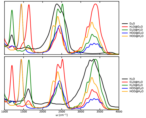
Figure 4: (Colour online) The infrared spectrum in the isotopic mixtures H₂O@D₂O, D₂O@H₂O, HOD@D₂O and HOD@H₂O.

3.3 Dependence on the coordination in the hydrogen bond network

We start the analysis from the average intramolecular O-H bond lengths, shown in table 2 in the different HB coordinations $C_{\mathrm{HB}}$ on the constrained, central molecule. The main effects are as expected: an O-H bond becomes elongated when a HB is donated by this OH group, and more so when there are more accepted HBs on the O since that weakens the intramolecular O-H bond strength. We have also evaluated the average dipole moment on the central molecule $\overline{D}$ via localization on Wannier functions. Here, we clearly see how the dipole moment increases upon having more HBs formed except the cases where the molecule accepts three HBs.

Table 2: Average intramolecular bond lengths and dipole moment in the constrained simulations.

$C_{\mathrm{HB}}$	$d(\mathrm{OH}_{a})$ [Å]	$d(\mathrm{OH}_{b})$ [Å]	$\overline{\mu}_{\mathrm{W}}$ [D]
A0D00	0.975$\pm$0.024	0.975$\pm$0.024	2.06
A0D01	0.975$\pm$0.023	0.984$\pm$0.024	2.23
A0D11	0.981$\pm$0.026	0.981$\pm$0.025	2.29
A1D00	0.976$\pm$0.025	0.976$\pm$0.025	2.38
A1D01	0.975$\pm$0.021	0.991$\pm$0.028	2.65
A1D11	0.986$\pm$0.028	0.986$\pm$0.028	2.78
A2D00	0.977$\pm$0.024	0.977$\pm$0.024	2.46
A2D01	0.976$\pm$0.024	0.997$\pm$0.028	2.80
A2D11	0.992$\pm$0.028	0.992$\pm$0.028	3.07
A2D11s	0.997$\pm$0.029	0.997$\pm$0.029	3.20
A3D11	0.995$\pm$0.030	0.993$\pm$0.027	2.97
A3Dnm	0.991$\pm$0.029	0.991$\pm$0.027	2.97

We determine how well the constraint on the HB coordination works by evaluating the distribution of $C_{\mathrm{HB}}$; the results are shown in figure 5b. Overall the central molecule is coordinated as given by the constraint, yet some differences occur, in particular in cases where the forcing of a given coordination leads to a strong difference in the number of acceptor and donor HBs from the “standard” coordination A₂D₁₁, such as A₂D₀₀. The distributions in the unconstrained trajectories, shown in figure 5a, indicate which coordinations naturally occur in the water: They are always close to the full coordination A₂D₁₁, sometimes having one accepting HB more or less (A₃D₁₁, A₁D₁₁) or one donor HB less (A₂D₀₁, A₁D₀₁); configuations with either no acceptor or donor HBs are very rare.

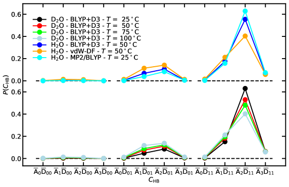
Figure 5: (Colour online) Distribution of HB configurations $C_{\mathrm{HB}}$ in the unconstrained trajectories.

The power spectrum of the constrained molecule, displayed in figure 6, gives indication of the frequency ranges in given coordinations. However, we concentrate on the frequency distributions yielded via the ENMA; these are also shown in figure 6, and the average frequencies of the two OH effective stretching modes in table 3.

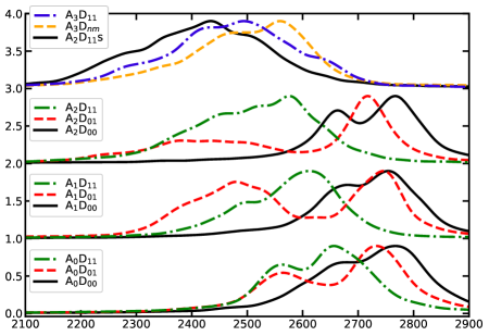
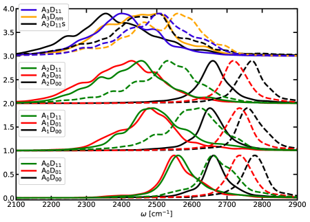
Figure 6: (Colour online) The power spectrum on the oxygen atoms (top panel) and the localized power spectra from ENMA (bottom panel) in the simulations with the restrained coordination of the hydrogen bonds.

Table 3: Frequencies obtained from localized ENMA vibrations at different coordinations $C_{\mathrm{HB}}$ on the central water molecule.

$C_{\mathrm{HB}}$	$\omega$			$\Delta\omega$
A0D00	1234	2686	2797	ref	ref	ref
A0D01	1224	2587	2756	$-10$	$-99$	$-41$
A0D11	1240	2628	2722	6	$-58$	$-74$
A1D00	1242	2678	2793	9	$-8$	$-4$
A1D01	1233	2500	2750	$-1$	$-186$	$-47$
A1D11	1230	2531	2628	$-4$	$-155$	$-168$
A2D00	1260	2678	2788	26	$-8$	$-9$
A2D01	1246	2428	2744	12	$-258$	$-52$
A2D11	1226	2449	2529	$-8$	$-237$	$-268$
A2D11s	1224	2431	2498	$-10$	$-255$	$-298$
A3D11	1204	2453	2529	$-30$	$-233$	$-268$
A3Dnm	1204	2453	2529	$-30$	$-233$	$-268$

A similar analysis is given in figure S16, where we have calculated the Fourier transform of the fluctuations of the intramolecular $d_{\mathrm{OH}}$ bond length and their average and difference, the latter mimicking a symmetric and asymmetric effective mode. These frequency distributions reflect well the ENMA modes, with a clear dual-peak structure in individual vibrations when one of the donor HBs is present and the other one is missing, yielding a breaking of the symmetry from the symmetric and asymmetric effective modes; correspondingly, the two peaks are better discerned in the average and difference of $d_{\mathrm{OH}}$ when both donor HBs are either present or broken; there, the symmetric and asymmetric effective modes provide a consistent picture of the local vibrations.

Against these observations it is easier to comprehend the changes upon varying coordination shown in the figure 7: When going from a quasi-free molecule $C_{\mathrm{HB}}=$A_nD₀₀ to A_nD₀₁ and to A_nD₁₁, the lower of the ENMA frequencies has its minimum in the middle configuration. This is probably caused by the collapse of the symmetric-asymmetric effective modes into two independent vibrations rather than an intrinsic lowest bond strength in those configurations.

Figure 7: (Colour online) Dependence of the two ENMA O-D stretching frequencies of a water molecule in D₂O in restricted coordinations upon a varying number of local number of acceptor and donor HBs.

We still make an observation of the hydrogen bond using the O-O-RDF split into contributions from hydrogen bonded and non-hydrogen bonded molecular pairs; the distributions are shown in figure S2. They appear as expected, with the major part of the first peak in the RDFs arising from hydrogen bonded molecules, and the non-hydrogen bonded pairs appearing at about 3.0 Å in the constrained samples and at about 2.7 Å in the normal trajectories. The amount of non-hydrogen bonds increases in D₂O upon increasing temperature, indicating more molecules penetrating into the first hydration shell of the molecules; we conclude that these are not hydrogen bonded to the central molecule since the share of the molecules with three acceptor HBs does not change in figure 5a.

4 Discussion

First of all, we remark that our overall description of the IR and Raman spectra of liquid water is relatively good: the main features and trends known from experiemets are very well reproduced qualitatively.

From earlier studies it has become apparent that the BLYP+D3 approach yields relatively realistic description of liquid water. Yet short-comings persist, like the too high equilibrium density at ambient conditions [6], the modest over-structuring of the liquid [13] arising due to a too high melting temperature [31] evidenced also in the collective vibrations [32].

When we compare our work to the previous literature on Raman spectra from structure method-based MD simulations [5], the agreement is reasonable, but we note that highly elevated temperature was used [5] in order to reduce the known tendency of over-structuring [33, 34] of the PBE treatment of XC.

Our simulated IR spectrum is very close to the one obtained earlier by Silvestrelli and Parrinello [3]. The reduction in the dipole moment upon an increased temperature is in line with the simulations of Guillot and Guissani [35]. The shifts in the shape of the Raman spectra are in line with those from the experiments and the neural networks [7].

In table 4 we compare the shifts in the OH/OD stretching frequency, defined as $\omega/\omega_{\mathrm{ref}}-1$, from our simulations in the D₂O with the constrained coordination to those obtained in [36] in HOD in D₂O. We note that the methods used are somewhat different, because in our simulations we obtain the frequencies from the analysis with the method ENMA, whereas in [36] the Authors use a semi-classical method, with the quantized dynamics on the single O-H bond; yet our goal is to quantify the trends on the shifts in the vibrational frequencies. Also in [36], the instantaneous configurations are grouped differently, where both the configurations labelled with $N_{\mathrm{O}}=1$ correpond to our cases A₀D_nm and A₀D_nm. As the $\omega_{\mathrm{ref}}$, we use the value in the coordination A₀D₀₀. We see the correspondence in the shifts, in particular, between the configurations A₁D₁₁ and 3_D and A₂D₁₁ and 4_D, and somewhat less clearly between the cases A₁D₀₁ and 2_SH. However, in the asymmetric coordinations A_nD₀₁, the two simulations differ more than in [36] where the central molecule is already asymmetric, namely HOD.

Table 4: Relative difference in the OH/OD stretching frequency at different coordinations of the hydrogen bonds both from our simulations and those from [36].

Coordination	$\omega$		shift		$N_{\mathrm{O}}$	$N_{\mathrm{H}}$	$N_{\mathrm{D}}$	label	shift
A0D00	2672	2786	ref	ref
A1D00	2700	2805	0.010	0.007	1	0	0	1N	$-$0.014
A2D00	2674	2778	0.001	$-$0.003	2	0	0	2N	$-$0.026
A0D01	2587	2743	$-$0.032	$-$0.015
A1D01	2512	2750	$-$0.060	$-$0.013	1	0	1	2SD	$-$0.011
					1	1	0	2SH	$-$0.067
A2D01	2588	2680	$-$0.031	$-$0.038	2	0	1	3SD	$-$0.022
					2	1	0	3SH	$-$0.088
A0D11	2579	2686	$-$0.035	$-$0.036
A1D11	2497	2590	$-$0.065	$-$0.071	1	1	1	3D	$-$0.063
A2D11	2457	2539	$-$0.080	$-$0.089	2	1	1	4D	$-$0.083

We note and admit here the admissions and unnecessary approximations and shortcuts in our simulations: in addition to the issues related to the approximative exchange-correlation functionals, neglected nuclear quantum effects, classical dynamics instead of the quantized dynamics, we also used a constant, empirical density of water instead of letting it adjust to the value that we would reach if the isothermal-isobaric ensemble were employed; indeed a density of 1.066 g/cm³ [37] has beeen found under the ambient conditions.

5 Conclusions

In this study we have performed DFT-based MD simulations of pure liquid water. We collected data on various structural and dynamical quantities, and we hope that the results will be useful in the interpretation of future investigations.

In particular, we investigated what happens to the O-H bond lengths, dipole moments and the vibrational frequencies when the coordination of the hydrogen bonds around the central molecules is different. We achieved this by explicitly restraining the distance of the neighbouring atoms from the oxygen and the two hydrogen or deuterium nuclei of the central molecule. We find definitive shifts in these quantities, which form the basis for the observations made in the normal, unconstrained simulations and thus further in the experimental results.

In the simulations of the liquid without constraints, we obtain an insight into the various underlying HB configurations in the course of simulations by correlating the characteristic frequency domain of the different HB coordination to the full spectrum in the fluctuating liquid. We can see how the numbers of the HBs reduce with the increased simulated temperature, yet interestingly the number of the configurations with five HBs — with our specific definition of an HB at least — is reduced only slightly whereas the average number of the HBs drops clearly.

In summary, we have managed to contribute somewhat further to the disclosure of the “secrets” of the hydrogen bond network and how the effects are detected in the experimental results.

Ukrainian 0

Ñïåêòðîñêîïiÿ êîëèâíèõ ñòàíiâ âîäè: òåìïåðàòóðíi òà êîîðäèíàöiéíi åôåêòè â êîìáiíàöiéíèõ òà iíôðàчåðâîíèõ ñïåêòðàõ Ð. Âóëåì’є${}^{\textsf{\footnotesize{\mbox{?}}}}$, A. Ï. Ñåéòñîíåí${}^{\textsf{\footnotesize{\mbox{?},\penalty 1000\mbox{?}}}}$

             
${}^{\textsf{\footnotesize 1}}$ Íàóêîâèé ïiäðîçäië ç âèâчåííÿ ïðîöåñiâ âèáiðêîâî¿ àêòèâàöi¿ íà îñíîâi îäíîåëåêòðîííî¿ àáî ðàäiàöiéíî¿ ïåðåäàчi åíåðãi¿ (PASTEUR), âiääiëåííÿ õiìi¿, Íîðìàëüíà âèùà øêîëà, Ïàðèçüêèé äîñëiäíèöüêèé óíiâåðñèòåò íàóê i ëiòåðàòóðè (PSL), Ñîðáîííñüêèé óíiâåðñèòåò, Íàöiîíàëüíèé öåíòð íàóêîâèõ äîñëiäæåíü (CNRS), F-75005 Ïàðèæ, Ôðàíöiÿ ${}^{\textsf{\footnotesize 2}}$ Iíñòèòóò õiìi¿, Öþðiõñüêèé óíiâåðñèòåò, Âiíòåðòóðåøòðàññå 190, CH-8057 Öþðiõ, Øâåéöàðiÿ

References

- [1] Perakis F., de Marco L., Shalit A., Tang F., Kann Z. R., Kühne T. D., Torre R., Bonn M., Nagata Y., Chem. Rev., 2016, 116, No. 13, 7590–7607, doi:10.1021/acs.chemrev.5b00640.
- [2] Resta R., J. Phys.: Condens. Matter, 2010, 22, 123201, doi:10.1088/0953-8984/22/12/123201.
- [3] Silvestrelli P. L., Bernasconi M., Parrinello M., Chem. Phys. Lett., 1997, 277, No. 5–6, 478–482, doi:10.1016/S0009-2614(97)00930-5.
- [4] Putrino A., Parrinello M., Phys. Rev. Lett., 2002, 88, 176401, doi:10.1103/PhysRevLett.88.176401.
- [5] Wan Q., Spanu L., Galli G. A., Gygi F., J. Chem. Theory Comput., 2013, 9, 4124–4130, doi:10.1021/ct4005307.
- [6] Ben M. D., Hutter J., VandeVondele J., J. Chem. Phys., 2015, 143, 054506, doi:10.1063/1.4927325.
- [7] Sommers G. M. Andrade M. F. C., Zhang L., Wang X., Car R., Phys. Chem. Chem. Phys., 2020, 22, 10592–10602, doi:10.1039/d0cp01893g.
- [8] Hohenberg P., Kohn W., Phys. Rev., 1964, 136, No. 3B, B864–B871, doi:10.1103/PhysRev.136.B864.
- [9] Lippert G., Hutter J., Parrinello M., Mol. Phys., 1997, 92, No. 3, 477–487, doi:10.1080/002689797170220.
- [10] VandeVondele J., Krack M., Mohamed F., Parrinello M., Chassaing T., Hutter J., Comput. Phys. Commun., 2005, 167, No. 2, 103–128, doi:10.1016/j.cpc.2004.12.014.
- [11] Kühne T. D., Iannuzzi M., Del B. M., Rybkin V. V., Seewald P., Stein F., Laino T., Khaliullin R. Z., Schütt O., Schiffmann F., J. Chem. Phys., 2020, 152, No. 19, 194103, doi:10.1063/5.0007045.
- [12] VandeVondele J., Mohamed F., Krack M., Hutter J., Sprik M., Parrinello M., J. Chem. Phys., 2005, 122, No. 1, 014515, doi:10.1063/1.1828433.
- [13] Jonchiere R., Seitsonen A. P., Ferlat G., Saitta A. M., Vuilleumier R., J. Chem. Phys., 2011, 135, 154503, doi:10.1063/1.3651474.
- [14] Goedecker S., Teter M., Hutter J., Phys. Rev. B, 1996, 54, No. 3, 1703, doi:10.1103/PhysRevB.54.1703.
- [15] Hartwigsen C., Goedecker S., Hutter J., Phys. Rev. B, 1998, 58, No. 7, 3641, doi:10.1103/PhysRevB.58.3641.
- [16] Becke A. D., Phys. Rev. A, 1988, 38, No. 6, 3098, doi:10.1103/PhysRevA.38.3098.
- [17] Lee C., Yang W., Parr R. G., Phys. Rev. B, 1988, 37, No. 2, 785, doi:10.1103/PhysRevB.37.785.
- [18] Grimme S., Antony J., Ehrlich S., Krieg H., J. Chem. Phys., 2010, 132, No. 15, 154104, doi:10.1063/1.3382344.
- [19] Lin I.-C., Seitsonen A. P., Coutinho-Neto M., Tavernelli I., Roethlisberger U., J. Phys. Chem. B, 2009, 113, No. 4, 1127–1131, doi:10.1021/jp806376e.
- [20] Perdew J. P., Burke K., Ernzerhof M., Phys. Rev. Lett., 1996, 77, No. 18, 3865, doi:10.1103/PhysRevLett.77.3865.
- [21] Dion M., Rydberg H., Schröder E., Langreth D. C., Lundqvist B. I., Phys. Rev. Lett., 2004, 92, No. 24, 246401, doi:10.1103/PhysRevLett.92.246401.
-
[22]
Murray É. D., Lee K., Langreth D. C., J. Chem. Theory Comput., 2009, 5, 2754–2762,
doi:10.1021/ct900365q. -
[23]
Lee K., Murray É. D., Kong L., Lundqvist B. I., Langreth D. C., Phys. Rev. B, 2010, 82, 081101,
doi:10.1103/PhysRevB.82.081101. -
[24]
Martinez M., Gaigeot M.-P., Borgis D., Vuilleumier R., J. Chem. Phys., 2006, 125, 144106,
doi:10.1063/1.2346678. - [25] Luber S., Iannuzzi M., Hutter J., J. Chem. Phys., 2014, 141, 094503, doi:10.1063/1.4894425.
- [26] Zhang C., Hutter J., Sprik M., J. Phys. Chem. Lett., 2016, 7, 2696–2701, doi:10.1021/acs.jpclett.6b01127.
- [27] Scherer J. R., Go M. K., Kint S., J. Phys. Chem., 1974, 78, 1304–1313, doi:10.1021/j100606a013.
- [28] Paolantoni M., Sassi P., Morresi A., Santini S., J. Chem. Phys., 2007, 127, 024504, doi:10.1063/1.2748405.
- [29] Maréchal Y., J. Mol. Struct., 2011, 1004, 146–155, doi:10.1016/j.molstruc.2011.07.054.
- [30] Linstrom P. J., Mallard W. G. (Eds.), NIST Chemistry WebBook, NIST Standard Reference Database Number 69, National Institute of Standards and Technology, 2023, doi:10.18434/T4D303.
- [31] Seitsonen A. P., Bryk T., Phys. Rev. B, 2016, 94, 184111, doi:10.1103/PhysRevB.94.184111.
- [32] Bryk T., Seitsonen A. P., Condens. Matter Phys., 2016, 19, 23604, doi:10.5488/CMP.19.23604.
- [33] Kuo I.-F. W., Mundy C. J., McGrath M. J., Siepmann J. I., VandeVondele J., Sprik M., Hutter J., Chen B., Klein M. L., Mohamed F., Krack M., Parrinello M., J. Phys. Chem. B, 2004, 108, No. 34, 12990–12998, doi:10.1021/jp047788i.
-
[34]
Lin I.-C., Seitsonen A. P., Tavernelli I., Roethlisberger U., J. Chem. Theory Comput., 2012, 8, 3902–3910,
doi10.1021/ct3001848. - [35] Guillot B., Guissani Y., In: Collision- and Interaction-Induced Spectroscopy, Vol. 114, Tabisz G. C., Neuman M. N. (Eds.), Kluwer Academic Publishers, Palo Alto, 1995, 129–142.
- [36] Auer B., Kumar R., Schmidt J. R., Skinner J. L., Proc. Natl. Acad. Sci. U.S.A., 2007, 104, 14215–14220, doi:10.1073/pnas.0701482104.
- [37] Ben M. D., Schönherr M., Hutter J., VandeVondele J., J. Phys. Chem. Lett., 2013, 4, 3753–3759, doi:10.1021/jz401931f.
Ukrainian \adddialect\l@ukrainian0 \l@ukrainian