Nonlocal approximation of minimal surfaces:
optimal estimates from stability

Abstract.

Minimal surfaces in closed 3-manifolds are classically constructed via the Almgren-Pitts approach. The Allen-Cahn approximation has proved to be a powerful alternative, and Chodosh and Mantoulidis (in Ann. Math. 2020) used it to give a new proof of Yau’s conjecture for generic metrics and establish the multiplicity one conjecture.

The primary goal of this paper is to set the ground for a new approximation based on nonlocal minimal surfaces. More precisely, we prove that if $\partial E$ is a stable $s$-minimal surface in $B_{1}\subset\mathbb{R}^{3}$ then:

• $\partial E\cap B_{1/2}$ enjoys a $C^{2,\alpha}$ estimate that is robust as $s\uparrow 1$ (i.e. uniform in $s$);

• the distance between different connected components of $\partial E\cap B_{1/2}$ must be at least of order $(1-s)^{\frac{1}{2}}$ (optimal sheet separation estimate);

• interactions between multiple sheets at distances of order $(1-s)^{\frac{1}{2}}$ are described by the Dávila–del Pino–Wei system.

A second important goal of the paper is to establish that hyperplanes are the only stable $s$-minimal hypersurfaces in $\mathbb{R}^{4}$, for $s\in(0,1)$ sufficiently close to $1$. This is done by exploiting suitable modifications of the results described above. In this application, it is crucially used that our curvature and separations estimates hold without any assumption on area bounds (in contrast to the analogous estimates for Allen-Cahn).

1. Introduction

The existence and regularity of minimal hypersurfaces is one of the central problems in Riemannian geometry. Particularly influential is the following question raised by S.-T. Yau [Yau82] in 1982:

Do all 3-manifolds contain infinitely many immersed minimal surfaces?

Since many 3-manifolds do not contain any area-minimizing surfaces, one needs to look for critical points (of the area functional). Such surfaces are naturally constructed by min-max —i.e., mountain-pass— methods, and are of finite Morse index.

The Almgren-Pitts approach

The most standard method for constructing min-max minimal surfaces is that of Almgren and Pitts [Pit81]. Building on it, Irie, Marques, and Neves [IMN18] gave in 2018 a positive answer to Yau’s conjecture in the case of generic metrics. Soon after, Song [Son18] was able to modify the methods from [IMN18] to establish the existence of infinitely many closed surfaces in every 3-manifold —thus positively answering Yau’s conjecture.

In the case of generic metrics, the results (multiplicity one and Morse index conjectures) established in [MR4172621, MR4191255] go far beyond Yau’s conjecture: for every integer $p\geqslant 1$ there exists an embedded minimal surface with index $p$ and area asymptotic to $c_{\circ}p^{1/3}$ (where $c_{\circ}$ is an explicit constant). However, when the same type of construction is run on manifolds that contain degenerate minimal surfaces (for generic metrics, this cannot happen), some information on the index of the constructed surfaces is lost. It seems complicated to understand in detail what is happening in these cases using the same methods. Thus, it is natural to ask if some alternatives to the Almgren-Pitts approach can provide complementary information.

The Allen-Cahn approach

Guaraco [MR3743704] proposed an alternative to the Almgren-Pitts theory, later extended by Gaspar–Guaraco [MR3814054]. Roughly speaking, the idea is to obtain minimal surfaces as limits as $\varepsilon\downarrow 0$ of (the zero level sets of) critical points of the Allen-Cahn functional:

$$J_{\varepsilon}(u):=\int_{M}\bigg{(}\varepsilon\frac{|\nabla u|^{2}}{2}+\frac{1}{\varepsilon}\frac{(1-u^{2})^{2}}{4}\bigg{)}d{\rm V}_{g},$$

where $(M,g)$ is a closed 3-manifold, $\nabla$ denotes the gradient on $M$, and ${\rm V}_{g}$ is the volume measure.

The connection between the Allen-Cahn functional and minimal surfaces has been long known: heuristically, the level sets of critical points of $J_{\varepsilon}$ converge to minimal surfaces as $\varepsilon\downarrow 0$ (see [MR0445362, MR1310848, MR1803974]). For fixed $\varepsilon>0$, critical points of $J_{\varepsilon}$ solve the following semilinear PDE (known as the Allen-Cahn equation):

$$-\Delta u=\varepsilon^{-2}(u-u^{3}).$$ (1.1)

Hence, thanks to elliptic regularity, for fixed $\varepsilon>0$, the set of all critical points of $J_{\varepsilon}$ is compact (in a very strong sense). This kind of strong compactness simplifies the construction of min-max critical points of $J_{\varepsilon}$ (defined on $H^{1}(M)$), making it comparable to the construction of critical points for Morse functions on finite dimensional manifolds (the Palais-Smale condition holds). In particular, from a technical viewpoint, the min-max construction for fixed $\varepsilon>0$ becomes much simpler than that in the Almgren-Pitts setting.

The following natural step is to send $\varepsilon\downarrow 0$ and try to recover minimal surfaces in the limit. However, this is hard since the nonlinearity in (1.1) blows up, and the elliptic estimates become useless. In [MR4045964], Chodosh and Mantoulidis succeeded in performing this delicate passage to the limit by carefully exploiting the finite Morse index property of min-max solutions. Among other things, they re-proved the existence of infinitely many minimal surfaces in closed 3-manifolds (with generic metrics) and established the multiplicity one conjecture of Marques and Neves. The most critical steps in their work are:

• Proving a (uniform in $\varepsilon$) curvature estimate for the level sets of stable critical points of $J_{\varepsilon}$ (assuming area bounds).

• Showing that whenever multiple sheets converge towards the same minimal surface, this limit must be degenerate (this requires a careful analysis of the interactions between different surface sheets encoded in the Toda system).

To achieve this, [MR4045964] builds on ideas developed by Wang and Wei in [MR3935478] to classify finite Morse index solutions of the Allen-Cahn equation in $\mathbb{R}^{2}$. For further information on the Allen-Cahn approximation of minimal surfaces, see also [MR4021161, DePhilippis-Pigati] and the references therein.

A new approach via nonlocal minimal surfaces

In [Yauforth], finite Morse index nonlocal minimal surfaces in a manifold are introduced and studied (see Section 1.1 here below for their definition). Surprisingly, these surfaces are in many respects better behaved than their classical (local) counterparts. For instance (see [Yauforth] for precise statements), the collection of all nonlocal minimal surfaces with index bounded by $m$ in a given closed $n$-manifold is compact in a very robust sense: In particular, any sequence has a subsequence that converges strongly in the natural Hilbert norm associated with nonlocal minimal surfaces. Therefore, roughly speaking, the “area” of the limit equals the limit of the “areas” although nonlocal minimal surfaces cannot have “multiplicity greater than one”. Moreover, in low dimensions ($n=3,4$), the collection of all nonlocal minimal surfaces with index bounded by $m$ is compact in the strongest possible sense, namely as “$C^{2}$ submanifolds”. Such strong compactness properties make nonlocal minimal surfaces particularly well-suited for min-max constructions. Indeed, in [Yauforth] the existence of infinitely many nonlocal minimal surfaces in any given close $n$-manifold is established —i.e., the nonlocal analog of Yau’s conjecture. This result is much less technical than in the case of classical minimal surfaces. Also, it works for all metrics and not just for generic ones.

Nonlocal minimal surfaces depend on a “fractional” parameter $s\in(0,1)$ —see Section 1.1 below. Similarly to the Allen-Cahn approach, classical minimal surfaces arise as a limit case: when the parameter $s$ approaches $1$. Thus, it is very natural to ask whether one can send $s\uparrow 1$ in the constructions from [Yauforth] to recover the classical Yau’s conjecture. As in the Allen-Cahn approach, two critical steps need to be addressed:

• Proving curvature estimates that are robust as $s\uparrow 1$.

• Extracting delicate information about interactions whenever multiple surface sheets converge towards the same limit surface.

This paper (see Theorem 1.1 below) addresses the aforementioned critical issues and thus sets the ground for the nonlocal approximation approach described above.

Although we address the most crucial steps, we do not give here a complete proof of the existence of infinitely many multiplicity one minimal surfaces (in close 3-manifolds with generic metric) using the new method because of two reasons. First, not to deviate from the paper’s central theme: i.e., proving optimal estimates for stable $s$-minimal surfaces in $\mathbb{R}^{3}$ (without assuming area bounds). Second, because —while it should now be relatively straightforward (using the results of this paper and [Yauforth], and adapting some ideas from [MR4045964]) to prove results analogous to those in [MR4045964] via nonlocal approximations— we expect that the new approach will yield to new (more precise) results that seem not achievable via Allen-Cahn. Thus, this will be worth investigating in depth in future works. In Section 1.5 below, we briefly discuss some possible advantages of the new approach and future directions.

Moreover, building on the new methods, we can address a central open problem in the theory of nonlocal minimal surfaces: we establish for the first time the classification of stable $s$-minimal cones in $\mathbb{R}^{4}$, for $s$ sufficiently close to $1$ (see Theorem 1.5 below).

1.1. Nonlocal minimal hypersurfaces

Nonlocal minimal (hyper)surfaces in $\mathbb{R}^{n}$ were introduced and first studied by Caffarelli, Roquejoffre, and Savin in [MR2675483]. Following this highly influential paper, several works extended (several parts of) the classical theory of minimal hypersurfaces to the new nonlocal setting —see, e.g., [MR3090533, CaffVal, BFV, FFMMM, MR3680376, MR3798717, MR3934589, MR4116635].

Nonlocal minimal hypersurfaces in a closed manifold

As said above, nonlocal minimal surfaces were initially defined in the Euclidean space $\mathbb{R}^{n}$ (in [MR2675483]). To study questions in Riemannian geometry, one needs a definition of nonlocal minimal surfaces on manifolds. The paper [Yauforth] gives a natural (canonic) definition that we recall next.

Let $n\geqslant 2$ and let $(M,g)$ be a closed $n$-dimensional Riemannian manifold.

Following the viewpoint of Caccioppoli and De Giorgi, (smooth, two-sided) minimal hypersurfaces in $M$ can be regarded as boundaries $\partial E$ of subsets $E\subset M$ which are critical points of the perimeter functional. Analogously, nonlocal (or fractional) minimal hypersurfaces in $M$ are defined as the boundaries $\partial E$ of subsets $E\subset M$ which are critical points of the fractional perimeter in $M$.

We first need to give a canonic definition of $H^{s/2}(M)$. As observed in [Yauforth], this can be done in at least three equivalent ways:

• Using the heat kernel $G(x,y,t)$ of $M$ we can set

  $$K_{s}(x,y):=\int_{0}^{\infty}G(x,y,t)\,\frac{dt}{t^{1+s/2}}.$$ (1.2)

  and

  $$[f]^{2}_{H^{s/2}(M)}:=\iint_{M\times M}(f(x)-f(y))^{2}K_{s}(x,y)\,d{\rm V}_{g}(x)\,d{\rm V}_{g}(y).$$ (1.3)

• Following a spectral approach, setting

  $$[f]^{2}_{H^{s/2}(M)}:=\sum_{k\geqslant 1}\lambda_{k}^{s/2}\langle f,\varphi_{k}\rangle^{2}_{L^{2}(M)},$$ (1.4)

  where $\varphi_{k}$ is an orthonormal basis of eigenfunctions of the Laplace-Beltrami operator $(-\Delta)_{M}$ and $\lambda_{k}$ are the corresponding eigenvalues.

• Using the Caffarelli-Silvestre extension, setting

  $$[f]^{2}_{H^{s/2}(M)}:=\inf\left\{\int_{M\times\mathbb{R}_{+}}z^{1-s}|\nabla_{x,z}F(x,z)|^{2}\,d{\rm V}_{g}(x)\otimes dz{\mbox{ s.t. }}F(\,\cdot\,,0)=f\right\}.$$

One can prove that (i)-(iii) define the same norm (not merely equivalent norms), up to multiplicative constants that we omit here —see [Yauforth] for the details. We emphasize the interest of having a canonic $H^{s/2}$ norm on a closed manifold (for instance, it seems that one cannot define a canonic $W^{s,1}$ norm on a manifold, as this type of norm can only be defined via charts and therefore will depend on the choice of an atlas and a partition of unity).

Now, the fractional perimeter in the closed manifold $M$ is defined as follows: given $s\in(0,1)$ and a (measurable) set $E\subset M$, we define

$$\mathrm{Per}_{s}(E):=(1-s)[\chi_{E}]^{2}_{H^{s/2}(M)},$$ (1.5)

where $\chi_{E}$ is the characteristic function of $E$.

One can see that, for every subset $E\subset M$ with smooth boundary, $(1-s)\mathrm{Per}_{s}(E)\to\mathrm{Per}(E)$ as $s\uparrow 1$ (up to a multiplicative dimensional constant, see [MR3586796] and also [MR1942130, MR2782803, MR2765717] for further details in the case of $\mathbb{R}^{n}$).

Given a set $E\subset M$ with smooth boundary, we say that $\partial E$ is $s$-minimal (or a critical point of $\mathrm{Per}_{s}$) if, for every smooth vector field $X$ on $M$, we have that

$$\frac{d}{dt}\Big{|}_{t=0}\mathrm{Per}_{s}(\phi^{X}(E,t))=0,$$ (1.6)

where $\phi^{X}:M\times\mathbb{R}\to M$ denotes the associated vector flow satisfying $\partial_{t}\phi^{X}=X\circ\phi^{X}$ and $\phi^{X}(x,0)=x$.

For the definition of stable and finite Morse index nonlocal minimal surfaces in $M$ —and criteria relating the Morse index and (almost-)stability for collections of disjoint subdomains— see [Yauforth].

Stable nonlocal minimal hypersurfaces in $\mathbb{R}^{n}$

By a suitable modification of (1.3)-(1.5), one can also define the fractional perimeter $\mathrm{Per}_{s}$ in $\mathbb{R}^{n}$, as well as on other non-compact, stochastically complete, Riemannian manifolds $\widetilde{M}$. For this, one needs to introduce relative fractional perimeters (e.g., we want to say that a hyperplane in $\mathbb{R}^{n}$ is a $s$-minimal surface even though a half-space has infinite $s$-perimeter).

Given a bounded open set $\Omega\subset\widetilde{M}$, a relative $s$-perimeter in $\Omega$ is a functional denoted by $\mathrm{Per}_{s}(\,\cdot,\Omega)$ and satisfying the following two properties:

• $\mathrm{Per}_{s}(E,\Omega)-\mathrm{Per}_{s}(F,\Omega)=\mathrm{Per}_{s}(E)-\mathrm{Per}_{s}(F)$ for all (measurable) sets $E$ and $F$ such that $E\setminus\Omega=F\setminus\Omega$ and $\mathrm{Per}_{s}(F)<\infty$.

• $\mathrm{Per}_{s}(E,\Omega)<\infty$ if $\partial E$ is a smooth submanifold in a neighbourhood of the compact set $\overline{\Omega}$.

A natural relative $s$-perimeter functional was defined in [MR2675483] as follows. Let for simplicity $\widetilde{M}=\mathbb{R}^{n}$ and notice that (1.2) makes complete sense in $\mathbb{R}^{n}$. As a matter of fact, a simple computation shows that $K_{s}(x,y)=|x-y|^{-n-s}$ (up to a multiplicative constant). Now, given a bounded open set $\Omega\subset\mathbb{R}^{n}$, put

$$\mathrm{Per}_{s}(E,\Omega):=(1-s)\iint_{(\mathbb{R}^{n}\times\mathbb{R}^{n})\setminus(\Omega^{c}\times\Omega^{c})}\frac{(\chi_{E}(x)-\chi_{E}(y))^{2}}{|x-y|^{n+s}}\,dx\,dy,$$

where $\Omega^{c}:=\mathbb{R}^{n}\setminus\Omega$. It is easy to show that, with this definition, properties (I) and (II) hold.

In this framework, we say that $\partial E$ is $s$-minimal in $\Omega$ if $\mathrm{Per}_{s}(E;\Omega)<\infty$ and (1.6) holds for all vector fields $X\in C^{\infty}_{c}(\Omega;\mathbb{R}^{n})$ (in other words if $E$ is a critical point of $\mathrm{Per}_{s}(\,\cdot\,,\Omega)$ with respect to $C^{2}$ inner variations not moving the complement of $\Omega$).

If, in addition, we have that

$$\frac{d^{2}}{dt^{2}}\Big{|}_{t=0}\mathrm{Per}_{s}(\phi^{X}(E,t),\Omega)\geqslant 0\quad\mbox{for all }X\in C^{\infty}_{c}(\Omega;\mathbb{R}^{n}),$$ (1.7)

then we say that $\partial E$ is stable (in $\Omega$).

Finally, we recall that $E$ is called a minimizer of $\mathrm{Per}_{s}(\,\cdot\,,\Omega)$ (and $\partial E$ is called a minimizing $s$-minimal hypersurface in $\Omega$) if

$$\mathrm{Per}_{s}(F,\Omega)\geqslant\mathrm{Per}_{s}(E,\Omega)\quad\mbox{for all $F\subset\mathbb{R}^{n}$ such that $F\setminus\Omega=E\setminus\Omega$}.$$

Minimizers are stable critical points (but not necessarily the other way around).

If $\partial E$ is assumed to be an $(n-1)$-submanifold of $\mathbb{R}^{n}$ of class $C^{2}$ in a neighborhood of the compact set $\overline{\Omega}$, then one can show (see [MR2675483, FFMMM]) that $\partial E$ is $s$-minimal in $\Omega$ if, and only if,

$$(1-s)\,{\rm p.v.}\int_{\mathbb{R}^{n}}\frac{(\chi_{E^{c}}-\chi_{E})(y)}{|x-y|^{n+s}}\,dy=0\quad\mbox{for all }x\in\partial E\cap\Omega.$$ (1.8)

Here above and in the rest of this paper, the notation “p.v.” stands for “in the principal value sense” (that is ${\rm p.v.}\int_{\mathbb{R}^{n}}\frac{(\chi_{E^{c}}-\chi_{E})(y)}{|x-y|^{n+s}}\,dy:=\lim_{r\downarrow 0}\int_{\mathbb{R}^{n}\setminus B_{r}(x)}\frac{(\chi_{E^{c}}-\chi_{E})(y)}{|x-y|^{n+s}}\,dy$). Equation (1.8) is called the $s$-minimal surface equation.

At this point, we have already introduced all the terminology needed for the paper’s main results. Thus we can proceed to state them.

1.2. Main results

Our first main result concerns robust (as $s\uparrow 1$) $C^{2,\alpha}$ estimates and optimal sheet separation estimates for stable $s$-minimal surfaces in $\mathbb{R}^{3}$ (generalizations to 3-manifolds hold with similar proofs, but we will focus on $\mathbb{R}^{3}$ for simplicity). It reads as follows:

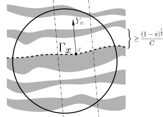
Figure 1. Sketch of the results in Theorem 1.1.

Theorem 1.1.

Let $E\subset\mathbb{R}^{n}$, with $n\in\{2,3\}$. There exist dimensional constants $s_{*}\in(0,1)$, $\alpha\in(0,1)$, $r_{\circ}\in(0,1)$, and $C>0$ such that the following holds true when $s\in[s_{*},1)$.

Suppose that $\partial E$ is a stable $s$-minimal set in $B_{2}$. Assume that $\partial E\cap B_{2}$ is an $(n-1)$-submanifold of class $C^{2}$ and let $\nu$ denote a unit normal vector field.

For any given $x\in\partial E\cap\overline{B_{1}}$, let $Y_{1},\dots,Y_{n}$ be an Euclidean coordinate system with origin at $x$ and $Y_{n}$-axis pointing in the $\nu(x)$ direction.

Let also $\Gamma_{x}$ be the connected component $\partial E\cap\{Y_{1}^{2}+\dots+Y_{n-1}^{2}\leqslant r_{\circ}^{2}\}$ containing $x$.

Let $g:B_{r_{\circ}}^{\prime}\to\mathbb{R}$ be such that $Y_{n}=g(Y_{1},\dots,Y_{n-1})$ on $\Gamma_{x}$.

Then,

$$\|g\|_{C^{2,\alpha}(B_{r_{\circ}}^{\prime})}\leqslant C.$$ (1.9)

Moreover, the following “sheet separation estimate” holds:

$$\partial E\cap\left\{Y_{1}^{2}+\dots+Y_{n-1}^{2}\leqslant r_{\circ}^{2}\;{\mbox{ with }}\;\big{|}Y_{n}-g(Y_{1},\dots,Y_{n-1})\big{|}\leqslant\frac{(1-s)^{\frac{1}{2}}}{C}\right\}=\Gamma_{x}.$$ (1.10)

A sketch of the result obtained in Theorem 1.1 is provided in Figure 1. Roughly speaking, Theorem 1.1 provides two precious pieces of information:

• The graph describing $\Gamma_{x}$ (which is assumed to be of class $C^{2}$, but only qualitatively) enjoys a $C^{2,\alpha}$ estimate that is robust as $s\uparrow 1$.

• While $\partial E$ can consist of many sheets, other sheets must be separated from $\Gamma_{x}$ by, at least, a distance  $\frac{(1-s)^{\frac{1}{2}}}{C}$, for a uniform $C>0$ as $s\uparrow 1$.

Remark 1.2.

The exponent $\frac{1}{2}$ in the “sheet separation estimate” (1.10) is sharp. Indeed, if, for example, one defines

$$E^{s}:=\bigcup_{k\in\mathbb{Z}}\left\{2k\leqslant\frac{x_{n}}{C_{*}\,\sqrt{1-s}}\leqslant 2k+1\right\},$$

then, by symmetry, $\partial E^{s}$ is a $s$-minimal set for all $s\in(0,1)$. Moreover, $\partial E^{s}$ is stable provided that $s$ is sufficiently close to $1$ and $C_{*}$ is chosen large enough (independently of $s$); see [newprep, Remark 2.3] for details.

Remark 1.3.

We emphasize that Theorem 1.1 can be regarded as the counterpart of the regularity theory developed by Chodosh-Mantoulidis [MR4045964] and Wang-Wei [MR4021161] in the context of Allen-Cahn approximations.

Remark 1.4.

The same result in Theorem 1.1 holds in dimension $n=4$ if we assume that $E$ has a conical structure with singularity away from the region of interest, e.g. under the assumption that $t(E-x_{\circ})=E-x_{\circ}$ for all $t>0$, for some $x_{\circ}$ with $|x_{\circ}|\geqslant 100$ (see Proposition 3.8 below). As we shall see, such an estimate plays a key role in the classification of stable $s$-minimal hypercones in $\mathbb{R}^{4}$ (see Theorem 1.5 below).

Our second main result classifies stable $s$-minimal cones in $\mathbb{R}^{4}$ for $s$ close to $1$:

Theorem 1.5.

There exists $s_{*}\in(0,1)$ such that for every $s\in(s_{*},1)$ the following holds true. Let $E\subset\mathbb{R}^{4}$ be a $s$-minimal hypercone that is stable in $\mathbb{R}^{4}\setminus\{0\}$. Suppose that $\partial E$ is nonempty and has a smooth trace on $\mathbb{S}^{3}$. Then, $\partial E$ must be a hyperplane.

The relation between Theorems 1.1 and 1.5 is that our proof of the latter result will critically rely on a version of the former one which applies to hypercones in $\mathbb{R}^{4}$ (recall Remark 1.4).

As a good example of the striking consequences that Theorem 1.5 entails, let us give the following:

Corollary 1.6.

Let $E\subset\mathbb{R}^{4}$ be a stable $s$-minimal surface and assume that $\partial E$ is smooth. If $s\in(s_{*},1)$, with $s_{*}$ as in Theorem 1.5, then $\partial E$ must be a hyperplane.

The analogue of Corollary 1.6 for $s=1$ was known as Schoen’s conjecture (see [ColdMin, Conjecture 2.12]). It states that any complete, connected stable minimal hypersurface in $\mathbb{R}^{4}$ must be a hyperplane, and has been proven only very recently by Chodosh and Li in the groundbreaking paper [ChoLi], with a completely different argument to the one that we employ here. It is interesting to point out that the results for $s\in(0,1)$ and for $s=1$ do not seem to imply each other in any way. In the next section, we explain why Theorem 1.5 implies Corollary 1.6 (here, one can glimpse a crucial feature of the nonlocal theory that is in marked contrast with the classical minimal surfaces theory).

1.3. Monotonicity formula and the fundamental role of hypercones

Nonlocal minimal hypersurfaces enjoy a monotonicity formula (which plays the role of Fleming’s monotonicity formula for minimal surfaces). This remarkable property, established by Caffarelli, Roquejoffre, and Savin [MR2675483], is formulated in terms of the Caffarelli-Silvestre extension $U_{E}$ of $\chi_{E^{c}}-\chi_{E}$. We recall that $U_{E}$ is defined as the (unique) bounded, weak solution $U$ of the problem

$$\begin{cases}{\rm div}(z^{1-s}\nabla U)=0\quad&\mbox{ in }\mathbb{R}^{n}\times(0,\infty),\\ U=\chi_{E^{c}}-\chi_{E}&\mbox{ on }\mathbb{R}^{n}\times\{0\},\end{cases}$$

where $\,{\rm div}\,$ and $\,\nabla\,$ are taken with respect to all $n+1$ coordinates $(x_{1},\dots,x_{n},z)$ of $\mathbb{R}^{n}\times(0,\infty)$.

As proven in [MR2675483], if $\partial E$ is a minimizing $s$-minimal hypersurface in $\Omega$, then, for all $x_{\circ}\in\partial E\cap\Omega$, the function

$$r\mapsto\phi_{E}(r,x_{\circ}):=r^{s-n}\int_{\widetilde{B}_{r}^{+}(x_{\circ})}z^{1-s}\,|\nabla U_{E}(x,z)|^{2}\,dx\,dz$$

is monotone nondecreasing in the interval $r\in(0,{\rm dist}(x_{\circ},\Omega^{c}))$. Here above, $\widetilde{B}_{r}^{+}(x_{\circ})$ denotes the upper half-ball of radius $r$ in $\mathbb{R}^{n+1}_{+}$ centered at $(x_{\circ},0)$. The proof in [MR2675483] easily generalizes to the case where $\partial E$ is any smooth stable $s$-minimal hypersurface in $\Omega$.

Moreover, $\phi_{E}(r,x_{\circ})$ is constant in $r$ in a neighbourhood of $0$ if, and only if, $E$ (or equivalently $\partial E$) is conical about $x$ —i.e. $t(E-x_{\circ})=E-x_{\circ}$ for all $t>0$.

A version of this monotonicity formula on Riemannian manifolds is found in [Yauforth].

As in the classical theory, the monotonicity formula confers a central role to $s$-minimal hypercones: every converging blow-up sequence ($R_{k}(E-x_{\circ})$, with $R_{k}\uparrow\infty$) or blow-down sequence ($r_{k}(E-x_{\circ})$, with $r_{k}\downarrow 0$) must have a conical limit. Thus, classifying minimizing or stable minimal cones is a crucial step in the regularity theory. Actually, in the nonlocal scenario, the classification of stable hypercones entails much stronger consequences than in the local ($s=1$) case. Indeed, for example, the following implication holds:

Theorem 1.7 ([newprep, Theorem 2.11]).

Assume that, for some pair $(n,s)$ with $n\geqslant 3$ and $s\in(0,1)$, hyperplanes are the only stable $s$-minimal hypercones in $\mathbb{R}^{n}\setminus\{0\}$.

Then, any stable $s$-minimal hypersurface $\partial E$ of class $C^{2}$ in $\mathbb{R}^{n}$ must be a hyperplane.

We notice that our Corollary 1.6 follows from a direct application of Theorems 1.5 and 1.7.

Theorem 1.7 can be informally stated as:

“Whenever one can prove flatness of stable $s$-minimal (hyper)cones, one can also prove flatness of any stable $s$-minimal hypersurface”.

So, the question is now: when can we prove that stable $s$-minimal cones in $\mathbb{R}^{n}$ must be flat?

For $s=1$, the answer to this question has been known since the late 1960s. Indeed, by the results of Almgren [Almgren], for $n=4$, and Simons [MR233295], for $5\leqslant n\leqslant 7$, we know that stable minimal cones are flat if $n\leqslant 7$. This is false for $n\geqslant 8$, “Simons’ cone” $\{x_{1}^{2}+x_{2}^{2}+x_{3}^{2}+x_{4}^{2}=x_{5}^{2}+x_{6}^{2}+x_{7}^{2}+x_{8}^{2}\}$ being a famous counterexample (as proven by Bombieri, De Giorgi, and Giusti [MR250205]).

By analogy to the $s=1$ case, for $s\in(0,1)$ it is natural to conjecture the following:

Conjecture 1.8.

For all $3\leqslant n\leqslant 7$, there exists $s_{*}\in(0,1)$ such that, for all $s\in(s_{*},1)$, hyperplanes are the only stable $s$-minimal hypercones in $\mathbb{R}^{n}\setminus\{0\}$.

Previously to this paper, Conjecture 1.8 had only been proven in dimension $n=3$ [MR4116635]. The same statement for minimizers is known in the whole dimensional range $3\leqslant n\leqslant 7$ [CaffVal]. Unfortunately, this approach for minimizers cannot be extended to general stable critical points. Here we establish the conjecture for $n=4$.

We must emphasize that for $s=1$ the analogue of the conclusion of Theorem 1.7 (i.e. the flatness of complete, connected embedded stable minimal hypersurfaces in $\mathbb{R}^{n}$ for $n\leqslant 7$) is a major open problem in dimensions $n=5,6,7$. Actually, the case $n=4$ was proven only very recently in [ChoLi] (for $n=3$ this has been known since the 1970’s  [MR546314, MR562550]).

Heuristically, the fact that the conclusion of Theorem 1.7 is so strong should put us on alert, and we should expect difficulties in establishing the validity of its assumptions. In order words, the problem of classifying nonlocal stable minimal hypercones must be highly non-trivial. Taking a naive approach, one would expect that sequences of stable $s_{k}$-minimal cones $\partial E_{k}$ should converge, as $s_{k}\uparrow 1$, towards some stable minimal hypercone (hence a hyperplane if $n\leqslant 7$ using Almgren and Simons’ result). However, turning this intuition into an actual mathematical proof poses several serious challenges; for instance:

• Nothing prevents, a priori, the sets $\partial E_{k}\cap\mathbb{S}^{n-1}$ from converging towards some subset of $\mathbb{S}^{n-1}$ with infinite $(n-2)$-perimeter!

• Even if we artificially added the assumption that $\sup_{k}\mathcal{H}^{n-2}(\partial E_{k}\cap\mathbb{S}^{n-1})<\infty$ (and even if we managed to use this extra information to prove that $\partial E_{k}$ should then converge towards a conical stable minimal integral varifold), the classification problem would remain far from trivial. Indeed, one would still need to rule out multiplicity of the limit surface: for instance $\partial E_{k}\cap\mathbb{S}^{n-1}$ could consist of several connected components all converging smoothly towards the “equator” of $\mathbb{S}^{n-1}$.

Remarkably, in this paper, we can rule out such scenarios in the $n=4$ case, thus establishing Conjecture 1.8 up to dimension $4$ (as stated in Theorem 1.5).

1.4. Multiplicity of the limit surface and the Dávila-del Pino-Wei system

As said above, ruling out multiplicity of the limit minimal surface is a key aspect of our proof of Conjecture 1.8 for $n=4$. On the other hand, the fine analysis of multiplicity situations is also critical to construct rich families of finite Morse index minimal surfaces: both using Allen-Cahn or nonlocal approximations. For these purposes, the information about “nonlocal interactions between sheets” becomes extremely valuable.

The following is a summary of our findings in this direction:

• As $s_{k}\uparrow 1$, multiple (even infinitely many) sheets of a sequence of $s_{k}$-minimal surfaces may converge towards the same smooth minimal surface (as explained in Remark 1.2, it is easy to construct examples where the number of sheets in a bounded region of space is of order $(1-s_{k})^{-\frac{1}{2}}\uparrow\infty$).

• When multiple sheets —at a critical distance of order $(1-s)^{\frac{1}{2}}$— are collapsing onto the same surface, crucial information on their nonlocal interactions “survives” in the limit $s\uparrow 1$. This information turns out to be encoded as a nontrivial solution of a certain (local!) PDE system of the following type:

  $$\Delta_{\mathbb{R}^{n-1}}\widetilde{g}_{i}=2\sum_{{1\leqslant j\leqslant N}\atop{j\neq i}}\frac{(-1)^{i-j}}{\widetilde{g}_{j}(x^{\prime})-\widetilde{g}_{i}(x^{\prime})},$$ (1.11)

  where $\widetilde{g}_{1}<\widetilde{g}_{2}<\dots<\widetilde{g}_{N}$ are functions from $\mathbb{R}^{n-1}$ to $\mathbb{R}$.

• This information, which can only be revealed through careful analysis, turns out to be essential in applications (e.g., in our proof of Conjecture 1.8 for $n=4$).

To the best of our knowledge, the system (1.11) was first considered in our context by Dávila, del Pino and Wei in [MR3798717], where embedded $s$-minimal surfaces with $N\geqslant 2$ layers (as well as $s$-catenoids, with $N=1$) are constructed. This construction is done by perturbing a particular solution of (1.11), as $s\uparrow 1$. More precisely, the “Ansatz”

$$\widetilde{g}_{i}=a_{i}\widetilde{g},\qquad i=1,\dots,N,$$

is made, where $\widetilde{g}:\mathbb{R}^{n-1}\to\mathbb{R}$ solves the Lane-Emden equation with negative exponent

$$\Delta_{\mathbb{R}^{n-1}}\widetilde{g}=\dfrac{1}{\widetilde{g}},$$ (1.12)

and $a_{i}\in\mathbb{R}$ satisfy the balancing condition

$$a_{i}=2\sum_{{1\leqslant j\leqslant N}\atop{j\neq i}}\frac{(-1)^{i-j}}{a_{j}-a_{i}},\qquad i=1,\dots,N.$$ (1.13)

While the construction in [MR3798717] is technically involved, no other properties of (1.11) are exploited. The model equation (1.12) has a longer history and has been studied for its various applications. The nonlinearity with negative exponent dates back to the 1970s and was studied in [Kawarada]. In geometrical contexts, this model has been used to construct singular minimal surfaces, see [Meadows, Simon]. The same equation has also been used in models of micro-electromechanical systems [MEMS] and thin film coating [Jiang-Ni]. Liouville-type results for entire stable solutions of (1.12) in the spirit of Farina [Farina] were obtained in [Ma-Wei].

Coming back to (1.11), the formal computations from [MR3798717] strongly suggest that a system of the type (1.11) should be the “right model” for interactions between sheets of rather general $s$-minimal surfaces as $s\uparrow 1$. However, to our knowledge, there were no rigorous results in this direction since the estimates that would be needed to bound the “errors” in the formal computations are very delicate (in particular, it does not seem possible to follow this approach for general $s$-minimal surfaces). Now, thanks to the strong $C^{2,\alpha}$ and optimal sheet separation estimates for stable surfaces that we obtain in this paper, we can rigorously estimate these errors.

More precisely, an example of the type of new results that we can prove is the following (see Lemma 3.9 for a more general statement): let $\Omega:=B_{1}^{\prime}\times(-1,1)\subset\mathbb{R}^{3}$, where $B_{1}^{\prime}$ is the unit ball of $\mathbb{R}^{2}$. Suppose that $\partial E_{k}$ is a sequence of stable $s_{k}$-minimal surfaces (in $\Omega$) with $s_{k}\uparrow 1$. Assume that $\partial E_{k}\cap\Omega=\bigcup_{i=1}^{N_{k}}\Gamma_{k,i}$ where $\Gamma_{k,i}:=\{x_{3}=g_{k,i}(x^{\prime})\}$, and $g_{k,1}<g_{k,2}<\dots<g_{k,N_{k}}$. Suppose in addition that $\sup_{1\leqslant i\leqslant N_{k}}\|g_{k,i}-g\|_{L^{\infty}(B_{1}^{\prime})}\to 0$ for some $g:B^{\prime}_{1}\to(-1,1)$. In other words, suppose that all the sheets of the surface $\Gamma_{k,i}$ are converging towards the same graphical surface $\Gamma:=\{x_{3}=g(x^{\prime})\}$. We stress that, in this assumption, the multiplicity (number of sheets converging to $\Gamma$) could be infinite as well. We also observe that, by the estimates in Theorem 1.1, we may assume that $\|g_{k,i}\|_{C^{2,\alpha}(B_{1}^{\prime})}$ is uniformly bounded for all $k$ and $i$ (and hence $g$ is $C^{2,\alpha}$). Then, under the above hypotheses, the following system of PDEs holds:

$$H[\Gamma_{k,i}](x)=2\sqrt{\sigma_{k}}\left(\sum_{j>i}(-1)^{i-j}\frac{\sqrt{\sigma_{k}}}{d(x,\Gamma_{k,j})}-\sum_{j<i}(-1)^{i-j}\frac{\sqrt{\sigma_{k}}}{d(x,\Gamma_{k,j})}\right)+O\big{(}(\sqrt{\sigma_{k}})^{1+\beta}\big{)},$$ (1.14)

where $x\in\Gamma_{k,i}$, $\sigma_{k}:=(1-s_{k})\downarrow 0$ and $\beta>0$. Here above, we have denoted by $H[\Gamma_{k,i}](x)$ the mean curvature of the surface $\Gamma_{k,i}$ at its point $x$, and by $d(x,\Gamma_{k,j})$ the distance in $\mathbb{R}^{3}$ between the point $x$ and the surface $\Gamma_{k,j}$.

We stress that, since we know from the optimal sheet separation estimate of Theorem 1.1 that $d(x,\Gamma_{k,j})\geqslant c\sqrt{\sigma_{k}}$, for some $c>0$, the error term $O\big{(}(\sqrt{\sigma_{k}})^{1+\beta}\big{)}$ in (1.14) is an honest higher-order term.

We also remark that in the particular case in which $N_{k}$ remains bounded, $g\equiv 0$ and

$$\widetilde{g}_{k,i}:=\frac{g_{k,i}}{\sqrt{\sigma_{k}}}\to\widetilde{g}_{i}\in L^{\infty}(B_{1}^{\prime})\quad\mbox{as $k\to+\infty$},$$

the limit of (1.14) as $k\to\infty$ is (1.11). Similarly, when multiple sheets converge towards some non-planar minimal surface, then a system like (1.11) is obtained, with the only difference that $\Delta_{\mathbb{R}^{n-1}}$ is replaced by the Jacobi operator of the minimal surface.

We also observe that the stability condition can be rewritten (see Proposition 4.11) in terms of solutions to the system (1.11), and one can use this to obtain non-existence of solutions. Additionally, we mention that the system (1.11) is analogous in many aspects to the Toda system for Allen-Cahn approximations, which plays a central role in [MR3935478, MR4021161, MR4045964].

1.5. Some advantages of the nonlocal approximation and future directions

As explained above, the primary motivation of this paper is to set the ground for the construction of minimal surfaces via nonlocal approximation. Let us comment briefly on the advantages that we see in this new approach:

• Obtaining the curvature estimate and the analog of Toda system is significantly more straightforward and less technical than using the Allen-Cahn approach. Indeed, this is done in Section 3 (which takes ca. 20 pages with an essentially self-contained presentation). Notice, however, that the most involved proof in Section 3 is that of Proposition 3.2 (it takes almost 10 pages). But Proposition 3.2 becomes almost trivial if one assumes area bounds (as the $L^{-2}$ estimate is then an immediate consequence of the stability inequality). Thus, if one is interested in the application to min-max, one can always proceed like in Allen-Cahn and prove a weaker curvature estimate depending on area bounds. Doing so, one can skip ca. 10 pages of the argument. Hence, in a fair comparison, one needs ca. 10 pages (of very detailed and largely self-contained proofs) to achieve results parallel to Allen-Cahn.

• Although this paper focuses on the case $n=3$, we do not discern any essential difficulty that could prevent one from extending the nonlocal approximation strategy to higher dimensions $4\leqslant n\leqslant 7$. A robust curvature estimate —depending on area bounds— for stable $s$-minimal surfaces in dimensions $4\leqslant n\leqslant 7$ will need to be developed (in particular, one will need a classification result for stable $s$-minimal cones for $s\sim 1$ depending on area bounds, which is a much weaker statement than Theorem 1.5). By comparison, the Allen-Cahn approximation seems much more difficult to extend to higher dimensions; the main obstruction being the absence of a classification result for stable solutions of the semilinear equation in $\mathbb{R}^{n}$ for $4\leqslant n\leqslant 7$ (even assuming area bounds!).

• Heuristically, one can think of nonlocal minimal surfaces as singular sets of critical points of the $H^{s/2}(M)$ energy among maps $M\to\mathbb{S}^{0}:=\{-1,+1\}$. From such a point of view, nonlocal minimal surfaces of codimension $d$ could be defined as the singular sets of critical points of $H^{(d-1)+s/2}(M)$ among maps $M\to\mathbb{S}^{d-1}$. First studied in [MR2783309], such maps are called fractional harmonic maps. They share several key properties with local and nonlocal minimal surfaces (e.g., they enjoy a monotonicity formula); see [MR4331016, MR3900821] and references therein. The current theory of fractional harmonic maps will need to be further developed if one aims to look at their singular sets as nonlocal minimal surfaces with higher codimension. This exciting direction will be pursued in future works.

• An exciting new feature of nonlocal approximations in contrast to Allen-Cahn is scaling invariance. Indeed, suppose that we have a sequence of $s_{k}$-minimal surfaces $\partial E_{k}$, with indexes bounded by $m$, and with $s_{k}\uparrow 1$ and some curvature of $\partial E_{k}$ blows-ups along the sequence. Then, one can consider a rescaled sequence converging towards a global minimal surface with finite Morse index in $\mathbb{R}^{3}$, and curvatures bounded by $1$. Such surfaces can be seen as “bubbles” that model “neck-type” singularities appearing when the approximating surfaces converge with multiplicity $>1$ to the same (degenerate) minimal surface. This type of analysis (which is not possible with the Allen-Cahn approximation because scaling changes the value of the parameter $\varepsilon$) can be very interesting to understand how exactly the index is lost in the presence of degenerate surfaces.

1.6. Acknowledgments

HC has received funding from the European Research Council under Grant Agreement No. 721675, grants CEX2019-000904-S funded by MCIN/AEI/ 10.13039/501100011033 and PID2020-113596GB-I00 by the Spanish government.

SD is supported by the Australian Research Council DECRA DE180100957 PDEs, free boundaries and applications.

JS is supported by the Swiss NSF Ambizione Grant PZ00P2 180042 and by the European Research Council under Grant Agreement No 948029.

EV is supported by the Australian Laureate Fellowship FL190100081 Minimal surfaces, free boundaries, and partial differential equations.

It is a pleasure to thank Alessandro Carlotto and Joaquín Pérez for interesting and helpful discussions concerning Lemma 4.5.

2. Overview of the proofs and organization of the paper

The rest of this paper is organized as follows.

• $C^{2,\alpha}$ and optimal separation estimates (Section 3)

  • Optimal separation in $L^{-2}$ (Proposition 3.2)

  • Decoupling of $s$-mean curvature equation (Proposition 3.5)

  • Optimal $L^{-\infty}$-separation in dimension $n=3$ (Proposition 3.5)

  • Robust $C^{2,\alpha}$ estimates in dimension $n=3$ (Proposition 3.8)

  • The limit Dávila-del Pino-Wei system of Toda type (Lemma 3.9)

  • Proof of Theorem 1.1 à la B. White (Section 3.7)

• Classification of stable $s$-minimal cones in $\mathbb{R}^{4}$ (Section 4)

  • Structure of embedded almost minimal surfaces on $\mathbb{S}^{3}$ with bounded second fundamental form (Lemma 4.5)

  • Graphical representation of trace of $s$-minimal cones on $\mathbb{S}^{3}$ (Proposition 4.6)

  • Limit Toda-type system (Proposition 4.9) and stability inequality (Proposition 4.11)

  • Proof of Theorem 1.5 in the spirit of A. Farina’s integral estimate (Section 4.5)

The paper ends with an appendix detailing some basic results about stability conditions for nonlocal minimal surfaces in bounded domains.

2.1. Main ideas in Section 3

Section 3 focuses on $C^{2,\alpha}$ and optimal separation estimates. We sketch next the main steps from the proofs in this part of the paper. In all steps before Step 6, a quantitative control on the second fundamental form of the stable $s$-minimal surface is assumed.

Step 1: Optimal separation in $L^{-2}$. One first obtains optimal separation estimates in Proposition 3.2, namely the following $L^{2}$ bound for the reciprocal of the distance between two consecutive sheets, described by the graphs of $x_{n}=g_{i}(x^{\prime})$ and $x_{n}=g_{i+1}(x^{\prime})$, of a stable $s$-minimal surface:

$$(1-s)\int_{B^{\prime}_{1/2}}\frac{dx^{\prime}}{|g_{i+1}-g_{i}|^{2}}\leqslant C.$$ (2.1)

This bound holds in any dimension and will be obtained through several bespoke integral estimates from the localized stability condition (precisely stated in Proposition 3.1)

$$(1-s)\iint_{\Gamma\times\Gamma}\frac{\big{|}\nu(x)-\nu(y)\big{|}^{2}\eta^{2}(x)}{|x-y|^{n+s}}\,d\mathcal{H}^{n-1}_{x}\,d\mathcal{H}^{n-1}_{y}\\ \leqslant(1-s)\iint_{\Gamma\times\Gamma}\negmedspace\frac{\big{(}\eta(x)-\eta(y)\big{)}^{2}}{|x-y|^{n+s}}\,d\mathcal{H}^{n-1}_{x}\,d\mathcal{H}^{n-1}_{y}+{\rm Ext}_{\Omega}^{2},$$ (2.2)

where $\Gamma=\partial E\cap\Omega$ and ${\rm Ext}_{\Omega}^{2}$ denotes the exterior term which accounts for the (nonlocal) interactions across $\partial\Omega$. Here $\Omega\subset B_{1}^{\prime}\times(-1,1)$ is an appropriately chosen cylindrical neighborhood of one of the sheets of the surface containing, at most, a large (but fixed) number of other sheets. In (2.1) we see that consecutive sheets of the surface interact, giving a positive contribution to the left-hand side to the stability inequality as the difference of the normal vectors for consecutive layers is of order $1$. This crucial information allows us to bound the left-hand side in the stability inequality (2.2) by below by a sum of the type

$$\sum_{i}(1-s)\int_{B^{\prime}_{1/2}}\frac{dx^{\prime}}{|g_{i+1}-g_{i}|^{2}}.$$

On the other hand, the integral on the right-hand side, and exterior term ${\rm Ext}_{\Omega}^{2}$, are bounded by double sums of the type

$$\sum_{i,j}(1-s)\int_{B^{\prime}_{1}}\frac{dx^{\prime}}{|g_{j}-g_{i}|^{2}}.$$

In order to relate the left and right hand sides we write $g_{j}-g_{i}$ as a telescoping sum and use the elementary inequality

$$\frac{1}{(g_{j}-g_{i})^{2}} \leqslant\frac{1}{(j-i)^{3}}\sum_{k=i}^{j-1}\frac{1}{(g_{k+1}-g_{k})^{2}}.$$

Doing so, and carefully using the smallness of certain constants appearing in the right hand side and appropriate covering arguments, one can close the estimate and prove (2.1). The details are given in the proof of Proposition 3.2.

Step 2: Decoupling. By singling out one layer from the others, the $s$-mean curvature equation can be decoupled and rewritten in terms of a quasilinear elliptic operator (Proposition 3.5), namely

$$H_{s}[\Gamma_{i}](x^{\prime},g_{i}(x^{\prime}))=(1-s)\int_{B^{\prime}_{1}}F\left(\frac{g_{i}(y^{\prime})-g_{i}(x^{\prime})}{|x^{\prime}-y^{\prime}|}\right)\,\frac{dy^{\prime}}{|x^{\prime}-y^{\prime}|^{n-1+s}}+O(1-s)=f_{i},$$ (2.3)

where $F(t)=c(n,s)\int_{0}^{t}(1+\tau^{2})^{-\frac{n+s}{2}}d\tau$.

Moreover, thanks to the separation estimate (2.1), the “remainders” $f_{i}$ are small in $L^{2}$ :

$$\left\|{f_{i}}\right\|_{L^{2}}\leqslant C\sqrt{1-s}.$$

As a matter of fact, a posteriori a more careful inspection of the “remainders” leads to the Toda-type system (1.11).

Step 3: Optimal $L^{-\infty}$-separation in dimension $n=3$. We proceed to show the sharp lower bound for the infimum of the distance between two consecutive layers, namely

$$\inf_{B_{1/2}^{\prime}}(g_{i+1}-g_{i})\geqslant c\sqrt{1-s}>0.$$ (2.4)

To this end, by taking the difference of equations (2.3) for two consecutive layers, we see that the separation $g_{i+1}-g_{i}$ satisfies a linearized elliptic equation

$$\mathcal{L}(g_{i+1}-g_{i})=H_{s}[\Gamma_{i+1}](x^{\prime},g_{i+1}(x^{\prime}))-H_{s}[\Gamma_{i}](x^{\prime},g_{i}(x^{\prime}))=\bar{f}_{i},\qquad\left\|{\bar{f}_{i}}\right\|_{L^{2}}\leqslant C\sqrt{1-s}.$$

The next step in Proposition 3.5 is to use Harnack inequality on the rescaled surfaces (zoom in by factor $1/r$) to obtain the linear growth bound on the separation:

$$(g_{i+1}-g_{i})(x_{\circ}^{\prime})=\delta\sqrt{1-s}\quad\implies\quad\sup_{B_{r/2}^{\prime}(x_{\circ}^{\prime})}(g_{i+1}-g_{i})\leqslant Cr\sqrt{1-s},\quad\forall r\in[\delta,1].$$

Inserting into (2.1), we easily obtain a contradiction in dimension $n=3$ if $\delta$ is small enough, using that the integral $\int_{\delta}^{1}\frac{r^{n-2}dr}{r^{2}}$ diverges as $\delta\downarrow 0$. Hence (2.4) must hold.

Step 4: $C^{2,\alpha}$ regularity in any dimension $n$. We observe that (2.3) can be seen as a uniformly nonlocal elliptic equation, where, by interpolation, the right-hand sides $f_{i}$ are uniformly bounded in $C^{\alpha}$ (Corollary 3.7). Thus, the local smoothness of $s$-minimal surfaces which are locally graphs [BFV] then gives robust $C^{2,\alpha}$ estimates (as $s\uparrow 1$) for $g_{i}$ (Proposition 3.8).

Step 5: Limit Toda-type system. As a consequence of these uniform $C^{2,\alpha}$ estimates (and layer separation bounds), rigorous Taylor expansions can be made to precisely estimate the nonlocal integrals. Doing so in Lemma 3.9 we will derive the elliptic system (1.14).

Step 6: Robust $C^{2,\alpha}$ estimates without quantitative $C^{2}$ bound. The preliminary results obtained in this way will thus be combined to a scaling trick due to Brian White and lead to the proof of Theorem 1.1. Roughly speaking, one aims at a uniform bound on the classical curvature of the stable $s$-minimal surface under consideration, and for that one argues by contradiction:

• If not, a suitable scaling $\Gamma_{k}$ of the sequence of surfaces with diverging curvature would maintain bounded (but nonzero) curvatures. Thus all estimates in Step 1 through Step 5, in particular uniform $C^{2,\alpha}$-compactness, are applicable to these rescalings.

• Any sub-sequential limit $\Gamma_{\circ}$ of $\Gamma_{k}$ is necessarily stable. If $\Gamma_{\circ}$ is isolated away from other limiting surfaces, one can pass the stability inequality to the limit. Otherwise, a positive Jacobi field can be constructed (from the normalized “distance” between the ordered surfaces, as in [ColdMin]).

• This would contradict the classical flatness of stable minimal surfaces in $\mathbb{R}^{3}$.

We stress that all these arguments vitally rely on the robust $C^{2,\alpha}$ estimates obtained in the previous steps.

2.2. Main ideas in Section 4

Then, in Section 4 we focus on the classification of stable $s$-minimal cones in $\mathbb{R}^{4}$. To this end, one analyzes the trace on the sphere $\mathbb{S}^{3}$ of stable $s$-minimal cones when $s$ is close to $1$:

Step 1: Structure of trace on $\mathbb{S}^{3}$ of $s$-minimal cones with bounded second fundamental form. The key reduction is to represent the trace of $s$-minimal cones on $\mathbb{S}^{3}$ as union of graphs over the equator (Proposition 4.6) with maximal height $O(\sqrt{1-s})$. To do this we first use a version for hypercones in $\mathbb{R}^{4}$ of the $C^{2,\alpha}$ estimate, combined with B. White’s blow-up strategy described above, in order to prove that the second fundamental form of the trace on the sphere of any stable $s$-minimal surface must be bounded by a constant independent of $s$ (as $s\uparrow 1$). This argument relies on the classification of complete embedded stable minimal surfaces in $\mathbb{R}^{3}$.

Also, in Lemma 4.5 we prove that any embedded $C^{2}$ almost minimal surface in $\mathbb{S}^{3}$ with bounded second fundamental form (not necessarily stable) must be a union of graphs over some closed minimal surfaces in $\mathbb{S}^{3}$ (here $n-1=3$ is also used because we need a universal area estimate for stable minimal immersion into $\mathbb{S}^{3}$ from [MR2483369]).

Finally, having shown that stable $s$-minimal hypercones in $\mathbb{R}^{4}$ are almost-minimal as $s\uparrow 1$ and have bounded second fundamental form, we deduce that their traces on $\mathbb{S}^{4}$ must accumulate towards the equator (up to rotation). Moreover, we prove that these spherical traces are a union of graphs over this equator with maximal height $O(\sqrt{1-s})$. Thanks to the optimal separation estimate we obtain, in addition, that the number of graphs is remains bounded as $s\uparrow 1$.

Step 2: Limiting Toda-type system and stability inequality. Once we know that, for $s$ sufficiently close to $1$, the trace of $s$-minimal cones on $\mathbb{S}^{n-1}$ is a union of graphs over its equator, $\bigcup_{i=1}^{N}\{x_{n}=g_{i}(\vartheta)\}$, with $\vartheta\in\mathbb{S}^{n-1}\cap\{x_{n}=0\}\cong\mathbb{S}^{n-2}$, $|g_{i}|\leqslant C\sqrt{1-s}$, and $\|g_{i}\|_{C^{2,\alpha}}\leqslant C$ (by the previous step we know it when $n=4$, but interestingly the last step actually works for $n\leqslant 7$), we can consider the re-normalized functions

$$\widetilde{g}_{i}:=\frac{g_{i}}{\sqrt{1-s}}.$$

We prove that these functions $\tilde{g}_{i}$, up to small errors,

• solve the Toda-type system (Corollary 4.10); and

• satisfy a stability condition (Corollary 4.13).

These results can be stated respectively as:

$$\Delta_{\mathbb{S}^{n-2}}\widetilde{g}_{i}(\vartheta)+(n-2)\widetilde{g}_{i}(\vartheta)=2\sum_{\begin{subarray}{c}1\leqslant j\leqslant N\\ j\neq i\end{subarray}}\frac{(-1)^{i-j}}{\widetilde{g}_{i+1}(\vartheta)-\widetilde{g}_{i}(\vartheta)}+O\bigl{(}(1-s)^{\gamma^{\prime}}\bigr{)},$$ (2.5)

$$\frac{2}{N}\sum_{\begin{subarray}{c}1\leqslant i<j\leqslant N\\ j-i\text{ odd}\end{subarray}}\int_{\mathbb{S}^{n-2}}\frac{4}{\big{|}\widetilde{g}_{j}(\vartheta)-\widetilde{g}_{i}(\vartheta)\big{|}^{2}}\,d{\mathcal{H}}^{n-2}_{\vartheta}\leqslant\frac{(n-3)^{2}+\varepsilon}{4}{\mathcal{H}}^{n-2}\big{(}\mathbb{S}^{n-2}\big{)}+C_{\varepsilon}(1-s)^{\gamma^{\prime}}.$$ (2.6)

The (small) parameter $\varepsilon>0$ in stability condition and the “numerology” $\frac{(n-3)^{2}}{4}$ comes from the fact that we choose a radial test function similar to $r^{-\frac{(n-1)-2}{2}}$ which almost saturates the (classical) Hardy’s inequality in $\mathbb{R}^{n-1}$.

Step 3: Classification of stable $s$-minimal cones in $\mathbb{R}^{4}$. One argues by contradiction (in the spirit of Alberto Farina) by testing the difference of two suitably chosen equations (2.5) against the reciprocal of the sheet separation and integrating by parts. This leads to a contradiction when compared to (2.6) as long as

$$(n-2)>\frac{(n-3)^{2}}{4},\quad\text{ i.e. }\quad 3\leqslant n\leqslant 7.$$

We point out that this dimensional range, which we believe to be optimal, is the same as in Simon’s celebrated result for $s=1$ in [MR233295]. This is interesting since, for Allen-Cahn approximations, the analogous dimensional range for the Toda system in [MR4021161] is $2\leqslant n-1\leqslant 9$, which does not correspond to the “natural” geometric dimensional range of minimal surfaces (in some sense the extra dimensions $n=8,9,10$ obtained for Allen-Cahn approximations are useless because the “bottleneck” is elsewhere).

3. $C^{2,\alpha}$ and optimal separation estimates

In this section, we prove that any stable $s$-minimal hypersurface such that the norm of its second fundamental form is bounded by $1$ in $B_{1}$ must satisfy a $C^{2,\alpha}$ estimate which is robust as $s\uparrow 1$. In addition, we prove optimal interlayer separation estimates and, as a byproduct, optimal bounds for the classical perimeter of the set in $B_{1/2}$.

3.1. Notation and preliminaries

Throughout the paper, we denote

$$\hskip 156.49014pt\sigma:=1-s\qquad\quad\quad\mbox{ (hence, $\sigma\downarrow 0$ as $s\uparrow 1$)}.$$

Given $\Omega\subset\mathbb{R}^{n}$ smooth and bounded, we assume that $E$ is a critical point of ${\rm Per}_{s}$ inside $\Omega$ and that $\partial E\cap\Omega$ is a smooth submanifold of $\mathbb{R}^{n}$. We define the normal vector $\nu$ to $\partial E$ (inside $\Omega$) as the map $\nu:\partial E\cap\Omega\to\mathbb{S}^{n-1}$ for which we have

$$\nabla\chi_{E}=-\nu\mathcal{H}^{n-1}|_{\partial E\cap\Omega}\quad\mbox{inside }\Omega.$$ (3.1)

Also, we denote by $n_{\Omega}$ the outwards unit normal to $\Omega$ (we intentionally use very different notations for the two normal vectors $\nu$ and $n_{\Omega}$ since they play very different roles).

Given a smooth and oriented hypersurface $(\Gamma,\nu)$ in $\mathbb{R}^{n}$ and $x\in\Gamma$ we define the fractional mean curvature of $\Gamma$ at $x$ as

$$H_{s}[\Gamma](x):=\sigma\int_{\Gamma}\nu(y)\cdot\frac{y-x}{|y-x|^{n+s}}\,d\mathcal{H}^{n-1}_{y}.$$

Recall that $\partial E$ is $s$-minimal in $\Omega\subset\mathbb{R}^{n}$ if, for all $x\in\partial E\cap\Omega$, we have (1.8). By a simple integration by parts argument, using that

$$\frac{1}{|x-y|^{n+s}}=\frac{1}{s}\,{\rm div}_{y}\left(\frac{x-y}{|x-y|^{n+s}}\right),$$

we obtain the equivalent equation

$$H_{s}[\partial E\cap\Omega](x)={\rm Ext}_{1}^{\Omega}(x)\quad\mbox{for all }x\in\partial E\cap\Omega,$$ (3.2)

where

$${\rm Ext}_{1}^{\Omega}(x):=\sigma\left(\int_{E\cap\partial\Omega}n_{\Omega}(y)\cdot\frac{x-y}{|x-y|^{n+s}}\,d\mathcal{H}^{n-1}_{y}+s\int_{E\cap\Omega^{c}}\frac{dy}{|x-y|^{n+s}}\right).$$

In this context, we have the following characterization of stability:

Proposition 3.1.

The stability of $\partial E$ in $\Omega$ is equivalent to the validity, for all $\eta\in C^{1}_{c}(\Omega)$, of

$$\sigma\iint_{\Gamma\times\Gamma}\frac{\big{|}\nu(x)-\nu(y)\big{|}^{2}\eta^{2}(x)}{|x-y|^{n+s}}\,d\mathcal{H}^{n-1}_{x}\,d\mathcal{H}^{n-1}_{y}\leqslant\sigma\iint_{\Gamma\times\Gamma}\negmedspace\frac{\big{(}\eta(x)-\eta(y)\big{)}^{2}}{|x-y|^{n+s}}\,d\mathcal{H}^{n-1}_{x}\,d\mathcal{H}^{n-1}_{y}+{\rm Ext}_{2}^{\Omega},$$ (3.3)

where $\Gamma:=\partial E\cap\Omega$ and

$${\rm Ext}_{2}^{\Omega}:=2\sigma\int_{\Gamma}d\mathcal{H}^{n-1}_{x}\,\eta^{2}(x)\nu(x)\cdot\left(\int_{E\cap\Omega^{c}}\frac{(n+s)(x-y)}{|x-y|^{n+s+2}}\,dy+\int_{E\cap\partial\Omega}\frac{n_{\Omega}(y)}{|x-y|^{n+s}}\,d\mathcal{H}^{n-1}_{y}\right).$$

The proof of this proposition is essentially given in the computations of the second variation of the fractional perimeter from [FFMMM]. We outline the modifications needed for our purposes in Appendix A.

To distinguish between vertical and horizontal components of a vector, we use the following notations. For $x\in\mathbb{R}^{n}$, we set $x=(x^{\prime},x_{n})$, where $x^{\prime}=(x_{1},\dots,x_{n-1})$; also we denote by $B_{1}^{\prime}$ the unit ball in $\mathbb{R}^{n-1}$.

In all this section we will assume that $n\geqslant 2$ and that $E\subset\mathbb{R}^{n}$ is a stable $s$-minimal set in

$$\Omega_{0}:=B_{1}^{\prime}\times(-1,1)\subset\mathbb{R}^{n}.$$

We will suppose, in addition, that

$$\partial E\mbox{ coincides with }\ \bigcup_{i=1}^{N}\,\{x_{n}=g_{i}(x^{\prime})\}\ \mbox{ inside }\Omega_{0},\quad{\mbox{for some }}g_{i}:B_{1}^{\prime}\to\mathbb{R}$$ (3.4)

$${\mbox{satisfying}}\quad g_{1}<g_{2}<\cdots<g_{N}\qquad\mbox{and}\qquad\|\nabla g_{i}\|_{L^{\infty}(B_{1}^{\prime})}+\|D^{2}g_{i}\|_{L^{\infty}(B_{1}^{\prime})}<\delta\,.$$ (3.5)

Here $N$ is some arbitrarily large positive integer. We will show that $N$ is bounded by a constant depending only on $n$ and $s$, but this constant blows up as $s\uparrow 1$ (in dimension $n=3$ we will actually show the optimal bound $N\leqslant C(1-s)^{-\frac{1}{2}}$). We emphasize that we do not make any quantitative assumption on the size of $N$, only a qualitative one (namely, that $N<+\infty$).

Also, $\delta>0$ in (3.5) will be chosen conveniently small in order to make some of the arguments easier. In latter applications we will always be able to assume that $\delta$ is small enough after zooming in around some point and making a suitable rotation.

We define $\Gamma_{i}:=\{x_{n}=g_{i}(x^{\prime})\}\cap\Omega_{0}$. We note that possibly $g_{i}(x^{\prime})\not\in(-1,1)$ for some $x^{\prime}\in B_{1}^{\prime}$, hence $\Gamma_{i}$ is not necessarily a graph over $B_{1}^{\prime}$.

We also denote

$$\Gamma:=\partial E\cap\Omega_{0}=\bigcup_{i=1}^{N}\Gamma_{i}.$$ (3.6)

We observe that, as a consequence of (3.2), if $i_{x}$ is such that $x\in\Gamma_{i_{x}}$ we have, for $\Omega_{0}=B_{1}^{\prime}\times(-1,1)$,

$$H_{s}[\Gamma_{i_{x}}](x)+\sum_{j\neq i_{x}}H_{s}[\Gamma_{j}](x)={\rm Ext}_{1}^{\Omega_{0}}(x)\quad\mbox{for all }x\in\Gamma.$$ (3.7)

3.2. Optimal separation estimate in $L^{-2}$

The goal of this subsection is to establish the following

Proposition 3.2.

There exists a dimensional constant $C>0$ such that the following holds true. Let $E$ be stable $s$-minimal in $B^{\prime}_{1}\times[-1,1]$ and assume that (3.4) and (3.5) hold true, with $(1-s)=\sigma\in(0,1/2)$ and $\delta:=\frac{1}{100}$.

Then, for every $i$ such that

$$\min_{\overline{B}_{1/2}^{\prime}}|g_{i}|\leqslant\frac{1}{2},$$ (3.8)

we have that

$$\sigma\int_{B^{\prime}_{1/2}}\frac{dx^{\prime}}{|g_{i+1}-g_{i}|^{2}}\leqslant C.$$

The result in Proposition 3.2 can be read as an estimate for the $L^{-2}$ norm of the separation (in the $x_{n}$ direction) of two consecutive graphs, that is for the function $(g_{i+1}-g_{i})$. By the example in Remark 1.2, the previous estimate is optimal. Since our final goal will be to obtain an estimate for the infimum of $(g_{i+1}-g_{i})$ (or equivalently for the $L^{-p}$ norm as $p\uparrow+\infty$), this can be seen as a first step in this direction.

To prove Proposition 3.2, we will need the following preliminary result.

Lemma 3.3.

Let $1-s=\sigma\in(0,1/2)$. Assume that for some $i<j$ we have $\min_{\overline{B_{1}^{\prime}}}(g_{j}-g_{i})\leqslant\widetilde{\delta}$ for some $\widetilde{\delta}>0$ and let

$$c_{n,s}:=\mathcal{H}^{n-2}(\mathbb{S}^{n-2})\int_{0}^{\infty}(1+t^{2})^{-\frac{n+s}{2}}\,t^{n-2}\,dt.$$

Then,

$$\big{(}1-c_{\delta,\widetilde{\delta}}\big{)}\frac{c_{n,s}\;\sigma}{|g_{j}(x^{\prime})-g_{i}(x^{\prime})|^{1+s}}\leqslant\int_{\Gamma_{j}}\frac{\sigma}{|x-y|^{n+s}}\,d\mathcal{H}^{n-1}_{y}\leqslant\big{(}1+c_{\delta,\widetilde{\delta}}\big{)}\frac{c_{n,s}\;\sigma}{|g_{j}(x^{\prime})-g_{i}(x^{\prime})|^{1+s}}$$

for all $x\in\Gamma_{i}\cap B_{3/4}^{\prime}\times\mathbb{R}$, where $c_{\delta,\widetilde{\delta}}\leqslant C(\sqrt{\delta}+\widetilde{\delta})\downarrow 0$ as $\delta,\widetilde{\delta}\downarrow 0$.

Proof.

In all the proof we may suppose without loss of generality that $\delta$ and $\widetilde{\delta}$ are conveniently small. Define

$$h(z^{\prime}):=g_{j}(x^{\prime}+z^{\prime})-g_{i}(x^{\prime}+z^{\prime})\geqslant 0$$

and notice that, since $\|D^{2}h\|_{L^{\infty}}\leqslant\|D^{2}g_{j}\|_{L^{\infty}}+\|D^{2}g_{i}\|_{L^{\infty}}\leqslant 2\delta$, we have

$$0\leqslant h(z^{\prime})=h(0)+Dh(0)\cdot z^{\prime}+\delta|z^{\prime}|^{2}\quad\mbox{for all $|z^{\prime}|\leqslant 1/4$}.$$ (3.9)

This yields that, for all $r\in(0,1/4)$,

$$|Dh(0)|=\frac{1}{r}\sup_{z^{\prime}\in B_{r}}(-Dh(0)\cdot z^{\prime})\leqslant\frac{1}{r}h(0)+\delta r$$

and hence, after optimizing in $r$,

$$|Dh(0)|\leqslant 2\sqrt{h(0)\delta}.$$ (3.10)

Let $\varrho:=\sqrt{h(0)}$. Then, using (3.9) and (3.10) we obtain

$$|h(z^{\prime})-h(0)|\leqslant|Dh(0)\cdot z^{\prime}|+\delta|z^{\prime}|^{2}\leqslant(2\sqrt{\delta}+\delta)\,h(0)=c_{\delta}\,h(0)\quad\mbox{for all }z^{\prime}\in B^{\prime}_{\varrho},$$

where $c_{\delta}:=2\sqrt{\delta}+\delta$, and therefore

$$(1-c_{\delta})h(0)\leqslant|h(z^{\prime})|\leqslant(1+c_{\delta})h(0)\quad\mbox{for all }z^{\prime}\in B^{\prime}_{\varrho}.$$

Now we want to estimate the quantity

$$\int_{\Gamma_{j}}\frac{\sigma}{|x-y|^{n+s}}\,d\mathcal{H}^{n-1}_{y}=\int_{\Gamma_{j}\cap B_{\varrho}(x)}\frac{\sigma}{|x-y|^{n+s}}\,d\mathcal{H}^{n-1}_{y}+\int_{\Gamma_{j}\setminus B_{\varrho}(x)}\frac{\sigma}{|x-y|^{n+s}}\,d\mathcal{H}^{n-1}_{y}.$$

For this, let $z:=y-x$. On the one hand, since $|g_{i}(y^{\prime})-g_{i}(x^{\prime})|\leqslant\delta|y^{\prime}-x^{\prime}|=\delta|z^{\prime}|$, we have

$$|y-x|^{2}=|y^{\prime}-x^{\prime}|^{2}+\big{(}g_{j}(y^{\prime})-g_{i}(x^{\prime})\big{)}^{2}$$

$$\qquad\quad=|z^{\prime}|^{2}+(h(z^{\prime})+O(\delta)|z^{\prime}|)^{2}=(|z^{\prime}|^{2}+h(0)^{2})(1+O(\delta)).$$

Using also that $d\mathcal{H}^{n-1}_{x}\leqslant\sqrt{1+\delta^{2}}\,dx^{\prime}$ on $\Gamma_{j}=\{x_{n}=g_{j}(x^{\prime}),|x^{\prime}|\leqslant 1\}$, we obtain (for some constant $c_{\delta}$ that may vary from line to line and satisfies $c_{\delta}\downarrow 0$ as $\delta\downarrow 0$) that

$$\begin{split}\int_{\Gamma_{j}\cap B_{\varrho}(x)}\frac{\sigma}{|x-y|^{n+s}}\,d\mathcal{H}^{n-1}_{y}&\leqslant(1+c_{\delta})\int_{\Gamma_{j}\cap B_{\varrho}(x)}\frac{\sigma}{\big{(}|x^{\prime}-y^{\prime}|^{2}+h(0)^{2}\big{)}^{n+s}}\,d\mathcal{H}^{n-1}_{y}\\ &\leqslant(1+c_{\delta})\int_{B^{\prime}_{\varrho}}\frac{\sigma}{\big{(}|z^{\prime}|^{2}+h(0)^{2}\big{)}^{n+s}}\,dz^{\prime}\\ &\leqslant(1+c_{\delta})\mathcal{H}^{n-2}(\mathbb{S}^{n-2})\sigma\int_{0}^{\infty}\frac{r^{n-2}\,dr}{(r^{2}+h(0)^{2})^{\frac{n+s}{2}}}\\ &\leqslant(1+c_{\delta})\frac{\mathcal{H}^{n-2}(\mathbb{S}^{n-2})\sigma}{h(0)^{1+s}}\int_{0}^{\infty}\frac{t^{n-2}\,dt}{(1+t^{2})^{\frac{n+s}{2}}}.\end{split}$$

On the other hand,

$$h(0)=|g_{j}(x^{\prime})-g_{i}(x^{\prime})|\leqslant\min_{\overline{B_{1}^{\prime}}}(g_{j}-g_{i})+2(\|\nabla g_{j}\|_{L^{\infty}}\|\nabla g_{i}\|_{L^{\infty}})\leqslant\widetilde{\delta}+4\delta\leqslant c_{\delta,\widetilde{\delta}}$$

and consequently $\frac{\varrho}{2h(0)}=\frac{\sqrt{h(0)}}{2h(0)}\to+\infty$ as $\delta,\widetilde{\delta}\downarrow 0$.

Additionally, if $\delta$ and $\widetilde{\delta}$ are sufficiently small, then $\Gamma_{j}\cap B_{\varrho}(x)$ will contain $\{x_{n}=g_{j}(x^{\prime})\ :\ x^{\prime}\in B_{\varrho/2}\}$. Therefore,

$$\begin{split}\int_{\Gamma_{j}\cap B_{\varrho}(x)}\frac{\sigma}{|x-y|^{n+s}}d\mathcal{H}^{n-1}_{y}&\geqslant(1-c_{\delta})\int_{\Gamma_{j}\cap B_{\varrho}(x)}\frac{\sigma}{\big{(}|x^{\prime}-y^{\prime}|^{2}+h(0)^{2}\big{)}^{n+s}}\,d\mathcal{H}^{n-1}_{y}\\ &\geqslant(1-c_{\delta})\int_{B^{\prime}_{\varrho/2}}\frac{\sigma}{\big{(}|z^{\prime}|^{2}+h(0)^{2}\big{)}^{n+s}}\,dz^{\prime}\\ &\geqslant(1-c_{\delta})\mathcal{H}^{n-2}(\mathbb{S}^{n-2})\sigma\int_{0}^{\varrho/2}\frac{r^{n-2}\,dr}{(r^{2}+h(0)^{2})^{\frac{n+s}{2}}}\\ &=(1-c_{\delta})\frac{\mathcal{H}^{n-2}(\mathbb{S}^{n-2})\sigma}{h(0)^{1+s}}\int_{0}^{\frac{\varrho}{2h(0)}}\frac{\bar{r}^{n-2}d\bar{r}}{(1+\bar{r}^{2})^{\frac{n+s}{2}}}\\ &\geqslant(1-c_{\delta,\widetilde{\delta}})\frac{\mathcal{H}^{n-2}(\mathbb{S}^{n-2})\sigma}{h(0)^{1+s}}\int_{0}^{\infty}\frac{t^{n-2}\,dt}{(1+t^{2})^{\frac{n+s}{2}}}.\end{split}$$

Finally, the contributions from “the exterior of the ball” can be bounded by

$$\begin{split}\left|\int_{\Gamma_{j}\setminus B_{\varrho}(x)}\frac{\sigma}{|x-y|^{n+s}}\,d\mathcal{H}^{n-1}_{y}\right|&\leqslant\int_{B_{2}^{\prime}\setminus B^{\prime}_{\varrho}(x)}\sqrt{1+\delta^{2}}\frac{\sigma}{|y^{\prime}-x^{\prime}|^{n+s}}\,dy^{\prime}\leqslant C\sigma\int_{\varrho}^{\infty}\frac{\bar{r}^{n-1}d\bar{r}}{\bar{r}^{n+s}}\\ &=C\frac{\sigma}{\varrho^{1+s}}=2C\frac{\sigma\delta}{h(0)^{\frac{1+s}{2}}}\leqslant c_{\delta,\widetilde{\delta}}\frac{\sigma}{h(0)^{1+s}}.\qed\end{split}$$

Before proving the optimal $L^{-2}$ estimate of Proposition 3.2, we establish next a rough (but helpful) estimate in $L^{-\infty}$.

Lemma 3.4.

With the same assumptions as in Proposition 3.2 we have

$$\inf_{B_{1/2}^{\prime}}(g_{i+1}-g_{i})\geqslant\frac{\sigma^{4}}{C}.$$

Proof.

Assume by contradiction that there exists a point $z^{\prime}\in B_{1/2}$ where $g_{i+1}-g_{i}=\tau^{2}\sigma^{4}$ for some $\tau\in(0,1)$. Our goal will be to bound $\tau$ away from zero (hence we may assume without loss of generality that $\tau$ is very small whenever needed).

By the assumption on $i$ in (3.8), we have that $|g_{i}(z^{\prime})|<3/4$. Let $z:=(z^{\prime},g_{i}(z^{\prime}))$ and $\varrho:=\tau\sigma^{2}$. Consider the rescaled set $\widetilde{E}:=(E-z)/\varrho$. We note that $\widetilde{E}$ is a stable $s$-minimal set in $B_{2}$. We also observe that the “layers” $\{x_{n}=g_{j}(x^{\prime})\}$ become, after scaling,

$$\{x_{n}=\widetilde{g}_{j}(x^{\prime})\}\qquad\mbox{where }\|D^{2}\widetilde{g}_{j}\|_{L^{\infty}}\leqslant\varrho\delta,\quad\mbox{for all }j=1,\dots,N.$$

Besides, since the point $z$ is mapped to $0$, we have that

$$\widetilde{g}_{i}(0)=0\quad\mbox{and}\quad\widetilde{g}_{i+1}(0)\leqslant\varrho.$$

It thereby follows, arguing similarly as in the proof of Lemma 3.3, that, for $\delta,\widetilde{\delta}$ sufficiently small,

$$0\leqslant\widetilde{g}_{i+1}-\widetilde{g}_{i}\leqslant 2\varrho\quad\mbox{in }B_{1}^{\prime}.$$

Now we use the stability inequality in Proposition 3.1 with $\Omega:=B_{1}$, $E$ replaced by $\widetilde{E}$, $\Gamma$ replaced by $\widetilde{\Gamma}:=\partial\widetilde{E}\cap B_{1}$, and $\eta$ any radial smooth cutoff satisfying $\chi_{B_{1/2}}\leqslant\eta\leqslant\chi_{B_{1}}$.

Using that $\widetilde{E}$ is stable $s$-minimal in $B_{2}$, the perimeter estimate in [MR4116635, Theorem 3.5] (see also [MR3981295, newprep]) gives that

$$\mathcal{H}^{n-1}(\widetilde{\Gamma})\leqslant\frac{C}{\sigma}.$$

Hence, we obtain the following bound for the right hand side of the stability inequality (that we denote here simply by “r-h-s”):

$$\mbox{r-h-s}:=\sigma\iint_{\widetilde{\Gamma}\times\widetilde{\Gamma}}\negmedspace\frac{\big{(}\eta(x)-\eta(y)\big{)}^{2}}{|x-y|^{n+s}}\,d\mathcal{H}^{n-1}_{x}\,d\mathcal{H}^{n-1}_{y}+{\rm Ext}_{2}^{\Omega}\leqslant\frac{C}{\sigma}.$$

Now, the left hand side in the stability inequality (that we denote by “l-h-s”) is

$$\mbox{l-h-s}:=\sigma\iint_{\widetilde{\Gamma}\times\widetilde{\Gamma}}\frac{\big{|}\widetilde{\nu}(x)-\widetilde{\nu}(y)\big{|}^{2}\eta^{2}(x)}{|x-y|^{n+s}}\,d\mathcal{H}^{n-1}_{x}\,d\mathcal{H}^{n-1}_{y}.$$

Using Lemma 3.3 and noticing that if $x\in\widetilde{\Gamma}_{i}$ and $y\in\widetilde{\Gamma}_{i+1}$ then $|\widetilde{\nu}(x)-\widetilde{\nu}(y)|\geqslant 2-c_{\varrho}\geqslant 1$, where $c_{\varrho}\downarrow 0$ as $\varrho\downarrow 0$, we conclude that

$$\int_{B_{1/4}^{\prime}}\frac{\sigma}{|g_{i+1}(x^{\prime})-g_{i}(x^{\prime})|^{1+s}}\,dx^{\prime}\leqslant C\,\mbox{l-h-s}.$$

From these considerations, and recalling that $|g_{i+1}(x^{\prime})-g_{i}(x^{\prime})|\leqslant 2\varrho$, we deduce

$$\frac{\sigma}{\varrho^{1+s}}\leqslant C\,\mbox{l-h-s}\leqslant C\,\mbox{r-h-s}\leqslant\frac{C}{\sigma}.$$

Since $\varrho=\tau\sigma^{2}$, from this we obtain that $\sigma^{-2s}\leqslant C\tau^{1+s}$. This yields that $\tau$ is bounded away from zero with a uniform bound for $\sigma\in(0,1/2)$ (actually the bound improves as $\sigma\downarrow 0$ since the quantity $\sigma^{-2s}\uparrow\infty$). This finishes the proof of Lemma 3.4. ∎

Proof of Proposition 3.2.

This proof is divided into several steps.

Step 1: Normalization. Observe first that, if we zoom in and choose a new coordinate frame about a point of the surface, the constant $\delta$ in (3.5) for the (suitably rotated) rescaled surface will became smaller. Hence, if we can prove the estimate in Proposition 3.2 assuming that (3.5) holds with $\delta>0$ tiny then the estimate in the case $\delta=\frac{1}{100}$ follows by a simple scaling and covering argument (with a larger constant $C$). Thus, let us assume without loss of generality that (3.5) holds with some $\delta>0$ to be chosen later.

Let

$$M :=\min\big{\{}j\geqslant i_{0}:\ \min_{\overline{B^{\prime}_{1}}}(g_{j+1}-g_{j})>2\delta\big{\}}$$

$${\mbox{and }}\quad m :=\min\big{\{}j\leqslant i_{0}:\ \max_{\overline{B^{\prime}_{1}}}(g_{j}-g_{j-1})>2\delta\big{\}}.$$

If the set of indices $j$ in the definition of $M$ (respectively $m$) is empty, we set $M:=N-1$ (respectively $m:=1$).

Recall that we denote $\Gamma=\bigcup_{1\leqslant i\leqslant N}\Gamma_{i}\subset\Omega_{0}=B_{1}^{\prime}\times(-1,1)$. For $x\in\Gamma$ we define

$$r_{x}:=\min\big{\{}1-|x^{\prime}|,1-|x_{n}|\big{\}}.$$

Let us define the “rescaled objects” $E_{x}:=\frac{1}{r_{x}}(E-x)$, $\Gamma_{i,x}:=\frac{1}{r_{x}}(\Gamma_{i}-x)\cap\Omega_{0}$, and $g_{i,x}:=\frac{1}{r_{x}}g_{i}(x^{\prime}+r_{x}\,\cdot\,)|_{B_{1}^{\prime}}$. Also, given $x\in\Gamma$ let $i_{x}$ be the index such that $x\in\Gamma_{i_{x}}$ and

$$M_{x,kN_{\circ}} :=\min\big{\{}i_{x}+kN_{\circ},M\big{\}}$$

$${\mbox{and }}\quad m_{x,kN_{\circ}} :=\max\big{\{}i_{x}+kN_{\circ},m\big{\}},$$

where $k\in\{1,3\}$ and $N_{\circ}$ is some (large) positive integer to be chosen later. We stress that $M$ and $m$ record the indices of first $2\delta$-separation in the largest scale (as $r_{x}\in(0,1]$) and remain the same for all rescalings.

Also, let us define $\varphi:\Gamma\to[0,\infty)$ as

$$\varphi(x):=\sum_{m_{x,N_{\circ}}\leqslant i<M_{x,N_{\circ}}}\int_{B^{\prime}_{1/2}}\frac{c_{n,s}\,\sigma\,dx^{\prime}}{|g_{i+1,x}-g_{i,x}|^{2}},$$

where $c_{n,s}$ is the positive constant from Lemma 3.3. Our goal will be to prove a bound of the type $\varphi(x)\leqslant C$ for all $x\in\Gamma$.

We first note that by definition $\varphi$ is upper-semicontinuous and $\varphi(x)\to 0$ as $x\to\partial\Omega_{0}$. Indeed, the upper-semicontinuity easily follows using that whenever $x_{k}\to x$ we have $\limsup_{k}[\overline{m}_{x_{k}},\overline{M}_{x_{k}}]=[\overline{m}_{x},\overline{M}_{x}]$, while the vanishing property of $\varphi$ on $\partial\Omega_{0}$ follows from observing that

$$\varphi(x)=\mathcal{H}^{n-1}(B_{1}^{\prime})r_{x}^{2}\sum_{m_{x,N_{\circ}}\leqslant i<M_{x,N_{\circ}}}\fint_{B^{\prime}_{r_{x}/2}(x^{\prime})}\frac{c_{n,s}\,\sigma\,dy^{\prime}}{|g_{i+1}-g_{i}|^{2}}$$

and $r_{x}\to 0$ as $x\to\partial\Omega_{0}$.

Hence, $\varphi$ attains a maximum at a point $x_{\circ}$ in the interior of $\Omega_{0}$. Now, by replacing the set $E$ by $E_{x_{\circ}}$ (and accordingly also $\Gamma_{i}$ and $g_{i}$ by $\Gamma_{i,x_{\circ}}$ and $g_{i,x_{\circ}}$ respectively) we may and do assume without loss of generality that $\varphi$ attains its maximum at $x_{\circ}=0$.

Step 2: Testing stability. We will now test the stability inequality (3.3) with a suitable test function. In order to define the test function let us set

$$\zeta_{i}:=\begin{cases}1\quad&\mbox{for }|i-i_{0}|\leqslant N_{\circ},\\ 2-\frac{|i-i_{0}|}{N_{\circ}}&\mbox{for }N_{\circ}\leqslant|i-i_{0}|\leqslant 2N_{\circ},\\ 0&\mbox{for }|i-i_{0}|\geqslant 2N_{\circ}\end{cases}$$ (3.11)

and

$$\overline{\zeta}_{i}:=\zeta_{i}\chi_{[m,M]}(i).$$

Also let $\zeta:B_{1}^{\prime}\times[-1,1]\to[0,1]$ be any Lipschitz function such that $\zeta=\overline{\zeta}_{i}$ on $\Gamma_{i}$ and let $\xi:\mathbb{R}^{n-1}\to\mathbb{R}$ some fixed smooth radial cutoff satisfying $\chi_{B^{\prime}_{1/2}}\leqslant\xi\leqslant\chi_{B^{\prime}_{3/4}}$.

Let us test the stability inequality (3.3) in the domain $\Omega$ defined as follows

$$\Omega =\big{\{}g_{i_{0}-3N_{\circ}}(x^{\prime})\leqslant x_{n}\leqslant g_{i_{0}+3N_{\circ}}(x^{\prime})\,,\ |x^{\prime}|\leqslant\tfrac{7}{8}\big{\}}\quad m\leqslant i_{0}-3N_{\circ} M\geqslant i_{0}+3N_{\circ}$$ if and (3.12)

$$\Omega =\big{\{}g_{m_{0}}(x^{\prime})-\delta\leqslant x_{n}\leqslant g_{i_{0}+3N_{\circ}}(x^{\prime})\,,\ |x^{\prime}|\leqslant\tfrac{7}{8}\big{\}} m>i_{0}-3N_{\circ} M\geqslant i_{0}+3N_{\circ}$$ if and (3.13)

$$\Omega =\big{\{}g_{i_{0}-3N_{\circ}}(x^{\prime})\leqslant x_{n}\leqslant g_{M_{0}}(x^{\prime})+\delta\,,\ |x^{\prime}|\leqslant\tfrac{7}{8}\big{\}} m\leqslant i_{0}-3N_{\circ} M<i_{0}+3N_{\circ}$$ if and (3.14)

$$\Omega =\big{\{}g_{m_{0}}(x^{\prime})-\delta\leqslant x_{n}\leqslant g_{M_{0}}(x^{\prime})+\delta\,,\ |x^{\prime}|\leqslant\tfrac{7}{8}\big{\}} m>i_{0}-3N_{\circ} M<i_{0}+3N_{\circ}$$ if and (3.15)

and with the test function (which is by construction compactly supported in $\Omega$)

$$\eta(x):=\xi(x^{\prime})\zeta(x).$$

Suppose now that $N_{\circ}$ and $\delta$ are chosen satisfying

$$8N_{\circ}\delta<\tfrac{3}{4}.$$ (3.16)

Then, we have that $x\in\Gamma$ and $\eta(x)>0$ imply

$$|x^{\prime}|<3/4\quad\mbox{and}\quad|x_{n}|\leqslant 3N_{\circ}\Big{(}\delta+{\rm diam}(B^{\prime}_{3/4})\|\nabla g_{i}\|_{L^{\infty}}\Big{)}\leqslant 8N_{\circ}\delta<\tfrac{3}{4}.$$

The stability inequality reads

$$I_{1}=\mbox{l-h-s}\leqslant\mbox{r-h-s}=I_{2}+I_{3},$$

where

$$I_{1}:=\sigma\iint_{(\Gamma\cap\Omega)\times(\Gamma\cap\Omega)}\frac{\big{|}\nu(x)-\nu(y)\big{|}^{2}\eta^{2}(x)}{|x-y|^{n+s}}\,d\mathcal{H}^{n-1}_{x}\,d\mathcal{H}^{n-1}_{y},$$

$$I_{2}:=\sigma\iint_{(\Gamma\cap\Omega)\times(\Gamma\cap\Omega)}\frac{\big{(}\eta(x)-\eta(y)\big{)}^{2}}{|x-y|^{n+s}}\,d\mathcal{H}^{n-1}_{x}\,d\mathcal{H}^{n-1}_{y},$$

and

$$I_{3}:={\rm Ext}_{2}^{\Omega}=2\sigma\int_{\Gamma\cap\Omega}\,d\mathcal{H}^{n-1}_{x}\eta^{2}(x)\nu(x)\cdot\left(\int_{E\cap\Omega^{c}}\frac{(n+s)(x-y)\,dy}{|x-y|^{n+s+2}}+\int_{E\cap\partial\Omega}\frac{n_{\Omega}(y)\,d\mathcal{H}^{n-1}_{y}}{|x-y|^{n+s}}\right).$$ (3.17)

Step 3: Estimate of $I_{1}$. We observe first that

$$2\varphi(0)\leqslant I_{1}.$$ (3.18)

Indeed, on the one hand if $(j-i)\in\{1,3,5,7\dots\}$ we have $|\nu_{j}(y)-\nu_{i}(x)|^{2}\geqslant 4(1-2\delta^{2})^{2}\geqslant 2$ (for $\delta$ sufficiently small) for all $i,j$. On the other hand, using Lemma 3.3 we obtain (also for $\delta$ sufficiently small)

$$\frac{c_{n,s}}{2}\frac{\sigma\,\xi(x^{\prime})^{2}}{|g_{i}(x^{\prime})-g_{j}(x^{\prime})|^{1+s}}\leqslant\int_{\Gamma_{j}}\frac{\sigma\,\xi(x^{\prime})^{2}}{|y-x|^{n+s}}\,d\mathcal{H}^{n-1}_{y}\leqslant 2c_{n,s}\frac{\sigma\,\xi(x^{\prime})^{2}}{|g_{i}(x^{\prime})-g_{j}(x^{\prime})|^{1+s}}$$ (3.19)

for all $x\in\Gamma_{i}$ with $x^{\prime}\in B_{3/4}^{\prime}$ and $m_{0}\leqslant i<j\leqslant M_{0}$. Furthermore, by Lemma 3.4, we have $(g_{j}-g_{i})\in(\sigma^{4}/C,1)$ for $j>i$ and hence —since $\lim_{\sigma\downarrow 0}\sigma^{\sigma}=1$— we find that $(g_{j}-g_{i})^{2}$ and $|g_{j}-g_{i}|^{1+s}$ are comparable with dimensional constants close to $1$, namely

$$|g_{j}-g_{i}|^{1+s}=\bigl{(}1+O(\sigma|\log\sigma|)\bigr{)}(g_{j}-g_{i})^{2}.$$ (3.20)

Therefore,

$$\begin{split}I_{1}&=\sigma\iint_{\Gamma\times\Gamma}\frac{\big{|}\nu(y)-\nu(x)\big{|}^{2}\eta^{2}(x)}{|y-x|^{n+s}}\,d\mathcal{H}^{n-1}_{x}\,d\mathcal{H}^{n-1}_{y}\\ &\geqslant 2\sum_{\begin{subarray}{c}m_{0,N_{\circ}}\leqslant i<j\leqslant M_{0,N_{\circ}}\\ (j-i)\text{ odd}\end{subarray}}\int_{B_{1}^{\prime}}\frac{c_{n,s}\,\sigma\,\xi(x^{\prime})^{2}\,dx^{\prime}}{|g_{j}(x^{\prime})-g_{i}(x^{\prime})|^{2}}\geqslant 2\sum_{m_{0,N_{\circ}}\leqslant i<M_{0,N_{\circ}}}\int_{B_{1}^{\prime}}\frac{c_{n,s}\,\sigma\,\xi^{2}\,dx^{\prime}}{|g_{i+1}-g_{i}|^{2}}.\\ \end{split}$$

Hence, (3.18) follows.

Step 4: Estimate of $I_{2}$. Our next goal is to bound from above $I_{2}$ and $I_{3}$. Let us start with $I_{2}$. Note that if $x\in\Gamma_{i}$ and $y\in\Gamma_{j}$ we have

$$\big{(}\eta(y)-\eta(x)\big{)}^{2}=(\xi(y^{\prime})\overline{\zeta}_{j}-\xi(x^{\prime})\overline{\zeta}_{i})^{2}\leqslant 2(\xi(y^{\prime})-\xi(x^{\prime}))^{2}\overline{\zeta}_{j}^{2}+2(\overline{\zeta}_{j}-\overline{\zeta}_{i})^{2}\xi^{2}(x^{\prime}).$$

Using this we can bound

$$I_{2}\leqslant I_{2,1}+I_{2,2}$$

where

$$I_{2,1}:=4\sigma\sum_{\begin{subarray}{c}i\leqslant j\\ \overline{\zeta}_{i}>0\end{subarray}}\iint_{\Gamma_{i}\times\Gamma_{j}}\frac{\big{(}\xi(y^{\prime})-\xi(x^{\prime})\big{)}^{2}}{|y-x|^{n+s}}\,d\mathcal{H}^{n-1}_{x}\,d\mathcal{H}^{n-1}_{y}$$

and

$$I_{2,2}:=4\sigma\sum_{\begin{subarray}{c}i<j\\ \Gamma_{i}\subset\Omega,\Gamma_{j}\subset\Omega\end{subarray}}(\overline{\zeta}_{j}-\overline{\zeta}_{i})^{2}\iint_{\Gamma_{i}\times\Gamma_{j}}\frac{\xi(x^{\prime})^{2}}{|y-x|^{n+s}}\,d\mathcal{H}^{n-1}_{x}\,d\mathcal{H}^{n-1}_{y}.$$

Now, on the one hand, by the definition of $\zeta_{i}$ , we notice that $\#\{i\ :\ \overline{\zeta}_{i}>0\}\leqslant 4N_{\circ}$. Hence, using that $|\xi(x^{\prime})-\xi(y^{\prime})|\leqslant C|x-y|$, one easily obtains

$$I_{2,1}\leqslant CN_{\circ}^{2}.$$

On the other hand, noticing that $\Gamma_{i}\subset\Omega$ if and only if $i\in[m_{0,3N_{\circ}},M_{0,3N_{\circ}}]$ and that $\overline{\zeta}_{i}=\zeta_{i}$ for all $i\in[m_{0,3N_{\circ}},M_{0,3N_{\circ}}]$, we obtain

$$I_{2,2}\leqslant 16c_{n,s}\sigma\sum_{m_{0,3N_{\circ}}\leqslant i<j\leqslant M_{0,3N_{\circ}}}(\zeta_{j}-\zeta_{i})^{2}\int_{B_{3/4}^{\prime}}\frac{\xi(x^{\prime})^{2}\,dx^{\prime}}{(g_{j}-g_{i})^{1+s}}.$$

In particular, by (3.20),

$$I_{2,2}\leqslant 16\sum_{m_{*}\leqslant i<j\leqslant M_{*}}(\zeta_{j}-\zeta_{i})^{2}\int_{B_{3/4}^{\prime}}\frac{c_{n,s}\,\sigma\,dx^{\prime}}{(g_{j}-g_{i})^{2}}.$$ (3.21)

Now setting $h_{i}:=g_{i+1}-g_{i}$ and noticing that the inequality between the harmonic and arithmetic means gives, at each $x^{\prime}\in B_{3/4}$,

$$\begin{split}\frac{1}{(g_{j}-g_{i})^{2}}&=\frac{1}{\left(\sum_{k=i}^{j-1}h_{k}\right)^{2}}=\frac{1}{(j-i)^{2}}\frac{(j-i)^{2}}{\sum_{k,\ell=i}^{j-1}h_{k}h_{\ell}}\leqslant\frac{1}{(j-i)^{2}}\frac{\sum_{k,\ell=i}^{j-1}\frac{1}{h_{k}h_{\ell}}}{(j-i)^{2}}\\ &\leqslant\frac{1}{(j-i)^{3}}\sum_{k=i}^{j-1}\frac{1}{h_{k}^{2}}=\frac{1}{(j-i)^{3}}\sum_{k=i}^{j-1}\frac{1}{(g_{k+1}-g_{k})^{2}}.\end{split}$$ (3.22)

Therefore, using (3.21) and recalling that $|M_{0,3N_{\circ}}-M_{0,3N_{\circ}}|\leqslant 6N_{\circ}$ and $|\zeta_{j}-\zeta_{i}|\leqslant\frac{|j-i|}{N_{\circ}}$, we obtain

$$\begin{split}I_{2,2}&\leqslant 16\sum_{m_{0,3N_{\circ}}\leqslant i<j\leqslant M_{0,3N_{\circ}}}\frac{(j-i)^{2}}{N_{\circ}^{2}}\int_{B_{3/4}^{\prime}}\frac{c_{n,s}\,\sigma\,dx^{\prime}}{(g_{j}-g_{i})^{2}}\\ &\leqslant 16\sum_{m_{0,3N_{\circ}}\leqslant i<j\leqslant M_{0,3N_{\circ}}}\frac{1}{N_{\circ}^{2}}\frac{1}{j-i}\sum_{k=i}^{j-1}\int_{B_{3/4}^{\prime}}\frac{c_{n,s}\,\sigma\,dx^{\prime}}{(g_{k+1}-g_{k})^{2}}\\ &\leqslant\frac{C\log N_{\circ}}{N_{\circ}}\sum_{m_{0,3N_{\circ}}\leqslant k<M_{0,3N_{\circ}}}\int_{B_{3/4}^{\prime}}\frac{c_{n,s}\,\sigma\,dx^{\prime}}{(g_{k+1}-g_{k})^{2}}.\end{split}$$ (3.23)

Step 5: Estimate of $I_{3}$. It only remains to bound $I_{3}={\rm Ext}_{2}^{\Omega}$. We need to consider 4 cases depending on which case in (3.12)-(3.15) applies. Consider first the case (3.12).

In this case we notice the test function $\eta$ is supported in

$$(B_{3/4}^{\prime}\times\mathbb{R})\cap\left(\bigcup_{|i-i_{0}|\leqslant 2N_{\circ}}\Gamma_{i}\right).$$ (3.24)

Now the dummy variable $x$ in the outer integral in (3.17) runs over a subset of the support of $\eta$, while in the inner integrals with respect to $y$ are integrated over a subset of the exterior of the domain $\Omega=\{g_{i_{0}-3N_{\circ}}(y^{\prime})\leqslant y_{n}\leqslant g_{i_{0}+3N_{\circ}}(y^{\prime}),|y^{\prime}|\leqslant\tfrac{7}{8}\}$.

We consider the (scalar) inner $y$-integral in the bulk

$$\begin{split}I_{3,1}:\!\!&=(n+s)\int_{E\cap\Omega^{c}}\frac{\nu(x)\cdot(x-y)}{|x-y|^{n+s+2}}\,dy.\end{split}$$ (3.25)

Since $x$ lies in the support (3.24), the kernel is uniformly bounded away from $0$ whenever $|y^{\prime}|\geqslant\tfrac{7}{8}$, giving

$$I_{3,1} =\int_{E\cap\Omega^{c}\cap B_{7/8}^{\prime}}(n+s)\frac{\nu(x)\cdot(x-y)}{|x-y|^{n+s+2}}\,dy+O(1).$$

In the vertical strip $|y^{\prime}|\leqslant\tfrac{7}{8}$, we decompose the exterior into

$$\Omega^{c}\cap B_{7/8}^{\prime}=\Omega^{c}_{+}\cup\Omega^{c}_{-},\quad\text{ where }\quad\Omega^{c}_{\pm}:=\{y\in\Omega^{c}\cap B_{7/8}^{\prime}:\pm\nu(x)\cdot(x-y)>0\}.$$

Here one of $\Omega^{c}_{+}$, $\Omega^{c}_{-}$ lies above $\Omega$ (with respect to the last coordinate) and the other below, depending on the orientation of $\nu(x)$. Hence,

$$|I_{3,1}| \leqslant C\left((n+s)\int_{E\cap\Omega^{c}_{+}}\dfrac{\nu(x)\cdot(x-y)}{|x-y|^{n+s+2}}\,dy-(n+s)\int_{E\cap\Omega^{c}_{-}}\dfrac{\nu(x)\cdot(x-y)}{|x-y|^{n+s+2}}\,dy+1\right)$$

$$\leqslant C\left((n+s)\int_{\Omega^{c}_{+}}\dfrac{\nu(x)\cdot(x-y)}{|x-y|^{n+s+2}}\,dy-(n+s)\int_{\Omega^{c}_{-}}\dfrac{\nu(x)\cdot(x-y)}{|x-y|^{n+s+2}}\,dy+1\right)$$

$$=C\left(\nu(x)\cdot\int_{\Omega^{c}_{+}}\nabla\left(\frac{1}{|x-y|^{n+s}}\right)\,dy-\nu(x)\cdot\int_{\Omega^{c}_{-}}\nabla\left(\dfrac{1}{|x-y|^{n+s}}\right)\,dy+1\right)$$

$$=C\left(\int_{\partial\Omega^{c}_{+}}\frac{\nu(x)\cdot n_{\Omega^{c}_{+}}(y)}{|x-y|^{n+s}}\,d\mathcal{H}^{n-1}_{y}-\int_{\partial\Omega^{c}_{-}}\frac{\nu(x)\cdot n_{\Omega^{c}_{-}}(y)}{|x-y|^{n+s}}\,d\mathcal{H}^{n-1}_{y}+1\right)$$

$$\leqslant C\left(\int_{\Gamma_{i_{0}+3N_{\circ}}}\dfrac{1}{|x-y|^{n+s}}\,d\mathcal{H}^{n-1}_{y}+\int_{\Gamma_{i_{0}-3N_{\circ}}}\dfrac{1}{|x-y|^{n+s}}\,d\mathcal{H}^{n-1}_{y}+1\right).$$

We observe that this upper bound also controls the other inner $y$-integral on the boundary:

$$I_{3,2}:=\int_{E\cap\partial\Omega}\frac{n_{\Omega}(y)\,d\mathcal{H}^{n-1}_{y}}{|x-y|^{n+s}} \leqslant C\left(\int_{\Gamma_{i_{0}+3N_{\circ}}}\dfrac{1}{|x-y|^{n+s}}\,d\mathcal{H}^{n-1}_{y}+\int_{\Gamma_{i_{0}-3N_{\circ}}}\dfrac{1}{|x-y|^{n+s}}\,d\mathcal{H}^{n-1}_{y}+1\right).$$

Using the previous observations we can easily bound —by a computation similar to the one in Lemma 3.3, and using again the observation (3.20)—

$$I_{3}={\rm Ext}_{2}^{\Omega} \leqslant C\sum_{|i-i_{0}|<2N_{\circ}}\left(\int_{B_{3/4}^{\prime}}\frac{c_{n,s}\,\sigma\,dx^{\prime}}{(g_{i_{0}+3N_{\circ}}-g_{i})^{2}}+\int_{B_{3/4}^{\prime}}\frac{c_{n,s}\,\sigma\,dx^{\prime}}{(g_{i}-g_{i_{0}-3N_{\circ}})^{2}}\right)+CN_{\circ}\sigma$$

$$\leqslant C\sum_{i=i_{0}-2N_{\circ}}^{i_{0}+2N_{\circ}-1}\int_{B_{3/4}^{\prime}}\dfrac{c_{n,s}\,\sigma\,dx^{\prime}}{(g_{i+1}-g_{i})^{2}}+CN_{\circ}\sigma.$$

Thus, making again use of (3.22) we obtain

$$I_{3}\leqslant CN_{\circ}\frac{1}{N_{\circ}^{3}}\sum_{k=i_{0}-3N_{\circ}}^{i_{0}+3N_{\circ}-1}\int_{B_{3/4}^{\prime}}\frac{c_{n,s}\,\sigma\,dx^{\prime}}{(g_{k+1}-g_{k})^{2}}+CN_{\circ}\sigma.$$

In the case (3.15) the estimate is actually simpler, because the top and bottom layers $\Gamma_{M}$ and $\Gamma_{m}$ are separated by a distance $\geqslant\delta$ from the top and bottom boundaries of the domain $\Omega$. Hence in this case it easily follows

$$I_{3}\leqslant C(\delta)N_{0}\sigma.$$

The two other cases (3.13) and (3.14) are a mixture of (3.12) and (3.15). In any case, for all the four cases we obtain the estimate

$$I_{3}\leqslant\frac{C}{N_{\circ}^{2}}\sum_{m_{0,3N_{\circ}}\leqslant k<M_{0,3N_{\circ}}}\int_{B_{3/4}^{\prime}}\frac{c_{n,s}\,\sigma\,dx^{\prime}}{(g_{k+1}-g_{k})^{2}}+C(\delta)N_{\circ}\sigma.$$ (3.26)

Step 6: Covering and conclusion. Putting together all of our previous estimates we obtain

$$2\varphi(0) \leqslant I_{1}\leqslant I_{2,1}+I_{2,2}+I_{3}$$

$$\leqslant CN_{\circ}^{2}+\left(\frac{C\log N_{\circ}}{N_{\circ}}+\frac{C}{N_{\circ}^{2}}\right)\sum_{m_{0,3N_{\circ}}\leqslant k<M_{0,3N_{\circ}}}\int_{B_{3/4}^{\prime}}\frac{c_{n,s}\,\sigma\,dx^{\prime}}{(g_{k+1}-g_{k})^{2}}+C(\delta)N_{\circ}\sigma.$$

Now, using the definition of $\varphi$ and the fact that it attains its maximum at $0$, a simple covering argument gives

$$\sum_{m_{0,3N_{\circ}}\leqslant k<M_{0,3N_{\circ}}}\int_{B_{3/4}^{\prime}}\frac{c_{n,s}\,\sigma\,dx^{\prime}}{(g_{k+1}-g_{k})^{2}}\leqslant C\varphi(0)+C(\delta)N_{\circ}\sigma.$$ (3.27)

In conclusion, we have

$$2\varphi(0)\leqslant CN_{\circ}^{2}+\left(\frac{C\log N_{\circ}}{N_{\circ}}+\frac{C}{N_{\circ}^{2}}\right)\varphi(0)+C(\delta)N_{\circ}\sigma,$$

provided that (3.16) holds.

Finally, we can choose first $N_{\circ}$ large enough in order to “absorb” $\frac{C\log N_{\circ}}{N_{\circ}}\varphi(0)$ and $\frac{C}{N_{\circ}^{2}}\varphi(0)$ in the left hand side and then choose $\delta>0$ sufficiently small so that (3.16) holds, obtaining

$$\varphi(0)\leqslant C(N_{\circ},\delta)=:C,$$

where $C$ is a constant depending only on $n$, as desired. ∎

3.3. Decoupling the equations: small right hand side in $L^{2}$

We now get back to the $s$-minimal surface equation (3.2). Using (3.7) and recalling the notation in (3.6), for fixed $i$ we will write it as

$$H_{s}[\Gamma_{i}](x)=-\sum_{j\neq{i}}H_{s}[\Gamma_{j}](x)+{\rm Ext}_{1}^{\Omega_{0}}(x)=:f_{i}(x),\quad\mbox{for all }x\in\Gamma_{i}.$$

While $H_{s}[\Gamma_{i}](x)$ only depends on “the geometry” of the layer (connected component of $\partial E$ in $\Omega_{0}$) $\Gamma_{i}$, since the $s$-minimal surface equation is nonlocal, all the different “layers” (i.e. different connected components of the boundary) interact in the equation through the right hand sides $f_{i}$. Surprisingly, as shown in the following proposition, the stability assumption yields that the interaction between layers is very small and the “system” becomes decoupled up to very small errors:

Proposition 3.5.

Let $s\in\left(\tfrac{1}{2},1\right)$ and $E$ be a stable $s$-minimal set in $B_{1}^{\prime}\times(-1,1)$. In the notation of (3.4), assume that

$$\|\nabla g_{i}\|_{L^{\infty}(B_{1}^{\prime})}+\|D^{2}g_{i}\|_{L^{\infty}(B_{1}^{\prime})}\leqslant\frac{1}{100}.$$ (3.28)

Then for every $i$ such that $\min_{\overline{B}_{1/2}}|g_{i}|\leqslant 1/2$ we have that

$$\|f_{i}\|_{L^{2}(\Gamma_{i}\cap B^{\prime}_{1/2}\times(-1,1))}\leqslant C\sqrt{\sigma}.$$ (3.29)

Moreover, in dimension $n=3$ we have the stronger estimates

$$\inf_{B^{\prime}_{1/2}}(g_{i+1}-g_{i})\geqslant c\sigma^{1/2}>0\quad\mbox{and}\quad\|f_{i}\|_{L^{\infty}(\Gamma_{i}\cap B^{\prime}_{1/2}\times(-1,1))}\leqslant C\sqrt{\sigma}.$$ (3.30)

Proof.

The proof consists of two steps.

Step 1. Let us show (3.29). Set $\Omega:=\Omega_{0}=B_{1}^{\prime}\times(-1,1)$. By (1.8), for all $x\in\Gamma_{i}$ we have that

$${\rm p.v.}\int_{\mathbb{R}^{n}}\frac{(\chi_{E^{c}}-\chi_{E})(y)}{|x-y|^{n+s}}\,dy=0.$$

Equivalently,

$${\rm p.v.}\int_{\Omega}\frac{(\chi_{E^{c}}-\chi_{E})(y)}{|x-y|^{n+s}}\,dy=-\int_{\Omega^{c}}\frac{(\chi_{E^{c}}-\chi_{E})(y)}{|x-y|^{n+s}}\,dy.$$

and therefore, for $|x^{\prime}|\leqslant\tfrac{1}{2}$,

$$\left|\sigma\,{\rm p.v.}\int_{\Omega}\frac{(\chi_{E^{c}}-\chi_{E})(y)}{|x-y|^{n+s}}\,dy\right|\leqslant\sigma\int_{\Omega^{c}}\frac{2}{|x-y|^{n+s}}\,dy\leqslant C\sigma.$$

In order to proceed with the estimate notice that in $\Omega$ we have that

$$E=\displaystyle\bigcup_{j\in 2\mathbb{Z}}\{g_{j-1}(x^{\prime})<x_{n}<g_{j}(x^{\prime})\}$$

and define the sets (for $i$ even; otherwise one changes the definitions accordingly)

$$\underline{F}_{i}:=\Omega\cap\{g_{i-1}(x^{\prime})<x_{n}<g_{i}(x^{\prime})\}\qquad\mbox{and}\quad\quad\overline{F}_{i}:=\Omega\setminus\{g_{i}(x^{\prime})<x_{n}<g_{i+1}(x^{\prime})\}$$

so that $\underline{F}_{i}\subset E\cap\Omega\subset\overline{F}_{i}$. We have

$${\rm p.v.}\int_{\Omega}\frac{(\chi_{{\overline{F}_{i}}^{c}}-\chi_{\overline{F}_{i}})(y)}{|x-y|^{n+s}}\,dy\leqslant{\rm p.v.}\int_{\Omega}\frac{(\chi_{E^{c}}-\chi_{E})(y)}{|x-y|^{n+s}}\,dy\leqslant{\rm p.v.}\int_{\Omega}\frac{(\chi_{{\underline{F}_{i}}^{c}}-\chi_{\underline{F}_{i}})(y)}{|x-y|^{n+s}}\,dy.$$

We now use that

$$\frac{1}{|x-y|^{n+s}}=\frac{1}{s}{\rm div}_{y}\left(\frac{x-y}{|x-y|^{n+s}}\right)$$

and hence for $x\in\Gamma_{i}$ with $|x^{\prime}|\leqslant\tfrac{1}{2}$,

$$\begin{split}&\quad\;\sigma\,{\rm p.v.}\int_{\Omega}\frac{(\chi_{{\overline{F}_{i}}^{c}}-\chi_{\overline{F}_{i}})(y)}{|x-y|^{n+s}}\,dy\\ &=\frac{\sigma}{s}\left(2\int_{\Omega\cap\partial\overline{F}_{i}}\dfrac{\nu(y)\cdot(x-y)}{|x-y|^{n+s}}\,d\mathcal{H}^{n-1}_{y}-\int_{\partial\Omega}\dfrac{(\chi_{\overline{F}_{i}^{c}}-\chi_{\overline{F}_{i}})(y)n_{\Omega}(y)\cdot(x-y)}{|x-y|^{n+s}}\,d\mathcal{H}^{n-1}_{y}\right)\\ &=\frac{2}{s}H_{s}[\Gamma_{i}](x)+\frac{2}{s}H_{s}[\Gamma_{i+1}](x)+O(\sigma)\end{split}$$

and similarly

$$\begin{split}&\quad\;\sigma\,{\rm p.v.}\int_{\Omega}\frac{(\chi_{{\underline{F}_{i}}^{c}}-\chi_{\underline{F}_{i}})(y)}{|x-y|^{n+s}}\,dy\\ &=\frac{\sigma}{s}\left(2\int_{\Omega\cap\partial\underline{F}_{i}}\dfrac{\nu(y)\cdot(x-y)}{|x-y|^{n+s}}\,d\mathcal{H}^{n-1}_{y}-\int_{\partial\Omega}\dfrac{(\chi_{\underline{F}_{i}^{c}}-\chi_{\underline{F}_{i}})(y)n_{\Omega}(y)\cdot(x-y)}{|x-y|^{n+s}}\,d\mathcal{H}^{n-1}_{y}\right)\\ &=\frac{2}{s}H_{s}[\Gamma_{i}](x)+\frac{2}{s}H_{s}[\Gamma_{i-1}](x)+O(\sigma).\end{split}$$

Therefore, for $x\in\Gamma_{i}$ with $|x^{\prime}|\leqslant\tfrac{1}{2}$ we have

$$-C\sigma+H_{s}[\Gamma_{i-1}](x)\leqslant H_{s}[\Gamma_{i}](x)\leqslant H_{s}[\Gamma_{i+1}](x)+C\sigma.$$ (3.31)

Now, as in Lemma 3.3 we observe that

$$\begin{split}\big{|}H_{s}[\Gamma_{i+1}](x)\big{|}&=\left|\sigma\int_{\Gamma_{i+1}}\nu(y)\cdot\frac{x-y}{|x-y|^{n+s}}\right|\leqslant\left|\sigma\int_{\Gamma_{j}}\frac{1}{|x-y|^{n+s-1}}\right|\\ &\leqslant\frac{C\sigma}{\big{|}g_{i+1}(x^{\prime})-g_{i}(x^{\prime})\big{|}^{s}}\leqslant\frac{C\sigma}{\big{|}g_{i+1}(x^{\prime})-g_{i}(x^{\prime})\big{|}}.\end{split}$$

Likewise,

$$\big{|}H_{s}[\Gamma_{i-1}](x)\big{|}\leqslant\frac{C\sigma}{\big{|}g_{i}(x^{\prime})-g_{i-1}(x^{\prime})\big{|}}.$$

Hence, using (3.31),

$$\big{|}H_{s}[\Gamma_{i}](x^{\prime},g_{i}(x^{\prime}))\big{|}\leqslant C\left(\frac{\sigma}{\big{|}g_{i+1}(x^{\prime})-g_{i}(x^{\prime})\big{|}}+\frac{\sigma}{\big{|}g_{i}(x^{\prime})-g_{i-1}(x^{\prime})\big{|}}\right).$$ (3.32)

Now we recall that by Proposition 3.2,

$$\big{\|}H_{s}[\Gamma_{i+1}]\big{\|}_{L^{2}(\Gamma_{i}\cap B^{\prime}_{1/2}\times(-1,1))}\leqslant C\left(\int_{B^{\prime}_{1/2}}\frac{\sigma^{2}\,dx^{\prime}}{\big{|}g_{i+1}(x^{\prime})-g_{i}(x^{\prime})\big{|}^{2}}\right)^{1/2}\leqslant C\big{(}C\sigma\big{)}^{1/2}\leqslant C\sqrt{\sigma}$$

and similarly,

$$\big{\|}H_{s}[\Gamma_{i-1}]\big{\|}_{L^{2}(\Gamma_{i}\cap B^{\prime}_{1/2}\times(-1,1))}\leqslant C\sqrt{\sigma}.$$

Hence using (3.31) we conclude that

$$\big{\|}H_{s}[\Gamma_{i}]\big{\|}_{L^{2}(\Gamma_{i}\cap B^{\prime}_{1/2}\times(-1,1))}\leqslant C\sqrt{\sigma}.$$ (3.33)

Step 2. Let us show (3.30). For this, we claim that, for $x^{\prime}\in B^{\prime}_{3/4}$ and $v:=(g_{i+1}-g_{i})\chi_{B_{1}^{\prime}}$, we have that

$$H_{s}[\Gamma_{i+1}](x^{\prime},g_{i+1}(x^{\prime}))-H_{s}[\Gamma_{i}](x^{\prime},g_{i}(x^{\prime}))=\sigma\int_{B^{\prime}_{1}}a_{i}(x,y)\frac{v(y^{\prime})-v(x^{\prime})}{|x^{\prime}-y^{\prime}|^{n-1+(1+s)}}\,dy^{\prime}+E(x^{\prime}),$$ (3.34)

where $\|E\|_{L^{\infty}(B^{\prime}_{3/4})}\leqslant C\sigma$ and $a_{i}$ is bounded from below away from zero and bounded from above.

To check this, we use equation (49) in [BFV] to see that

$$H_{s}[\Gamma_{i}](x^{\prime},g_{i}(x^{\prime}))=\sigma\int_{B^{\prime}_{1}}F\left(\frac{g_{i}(y^{\prime})-g_{i}(x^{\prime})}{|x^{\prime}-y^{\prime}|}\right)\,\frac{dy^{\prime}}{|x^{\prime}-y^{\prime}|^{n-1+s}}+O(\sigma),$$

where $F\in C^{1}(\mathbb{R})$ is such that $F(0)=0$ and

$$F^{\prime}(r)=\frac{c}{(1+r^{2})^{\frac{n+s}{2}}},$$ (3.35)

for some $c>0$.

Therefore,

$$H_{s}[\Gamma_{i+1}](x^{\prime},g_{i+1}(x^{\prime}))-H_{s}[\Gamma_{i}](x^{\prime},g_{i}(x^{\prime}))$$

$$= \sigma\int_{B^{\prime}_{1}}\left[F\left(\frac{g_{i+1}(y^{\prime})-g_{i+1}(x^{\prime})}{|x^{\prime}-y^{\prime}|}\right)-F\left(\frac{g_{i}(y^{\prime})-g_{i}(x^{\prime})}{|x^{\prime}-y^{\prime}|}\right)\right]\,\frac{dy^{\prime}}{|x^{\prime}-y^{\prime}|^{n-1+s}}+O(\sigma)$$

$$= \sigma\int_{B^{\prime}_{1}}F^{\prime}\big{(}\xi_{i}(x^{\prime},y^{\prime})\big{)}\Big{(}\big{(}g_{i+1}(y^{\prime})-g_{i+1}(x^{\prime})\big{)}-\big{(}g_{i}(y^{\prime})-g_{i}(x^{\prime})\big{)}\Big{)}\,\frac{dy^{\prime}}{|x^{\prime}-y^{\prime}|^{n-1+(1+s)}}+O(\sigma),$$

for some $\xi_{i}(x^{\prime},y^{\prime})$ lying on the segment joining $P_{i}:=\frac{g_{i}(y^{\prime})-g_{i}(x^{\prime})}{|x^{\prime}-y^{\prime}|}$ to $P_{i+1}:=\frac{g_{i+1}(y^{\prime})-g_{i+1}(x^{\prime})}{|x^{\prime}-y^{\prime}|}$. We stress that $|P_{i}|$ and $|P_{i+1}|$ are bounded uniformly, due to (3.28), therefore $a_{i}(x^{\prime},y^{\prime}):=F^{\prime}\big{(}\xi(x^{\prime},y^{\prime})\big{)}$ is bounded from below away from zero and bounded from above, thanks to (3.35), and the proof of (3.34) is complete.

From (3.33) and (3.34) it follows that

$$|\mathcal{L}v|\leqslant h\quad\mbox{in }B^{\prime}_{3/4},$$

where

$$\mathcal{L}v:=\sigma\int_{B^{\prime}_{1}}a_{i}(x^{\prime},y^{\prime})\frac{v(y^{\prime})-v(x^{\prime})}{|x^{\prime}-y^{\prime}|^{n-1+(1+s)}}\,dy^{\prime}$$

and $\|h\|_{L^{2}(B^{\prime}_{3/4})}\leqslant C\sqrt{\sigma}$. Note that the order of the operator is $1+s$, which is arbitrarily close to $2$.

Hence by the Harnack inequality for nonlocal operators (see [MR1941020, MR2095633]), if $q>n^{\prime}/(1+s)$, with $n^{\prime}:=n-1$, we have that

$$\sup_{B_{1/2}^{\prime}}v\leqslant C\inf_{B_{1/2}^{\prime}}v+C\|h\|_{L^{q}(B_{3/4}^{\prime})}.$$

For $n=3$ and $s\in\left(\tfrac{1}{2},1\right)$, we may take $q=2$, thus obtaining that

$$\sup_{B_{1/2}^{\prime}}(g_{i+1}-g_{i})\leqslant C\inf_{B_{1/2}^{\prime}}(g_{i+1}-g_{i})+C\sqrt{\sigma}.$$ (3.36)

Furthermore, in dimension $n=3$ (and thus $n^{\prime}=2$), assume now that $(g_{i+1}-g_{i})(x_{\circ}^{\prime})=\delta\sqrt{\sigma}$ for some $x^{\prime}_{\circ}\in B^{\prime}_{1/2}$ and let us prove a lower bound for $\delta$.

For $r\in(0,1/4)$ we now dilate the set $E$ around $x_{\circ}=(x_{\circ}^{\prime},g_{i}(x_{\circ}^{\prime}))\in\Gamma_{i}$ and we obtain new surfaces $\Gamma_{i,r}:=\frac{1}{r}(\Gamma_{i}-x_{\circ})$ which have graphical expressions $x_{n}=g_{i,r}(x^{\prime})$ in $B_{1}^{\prime}\times(-1,1)$, where $g_{i,r}(x^{\prime}):=\frac{1}{r}g_{i}(x_{\circ}^{\prime}+rx^{\prime})$.

Since (3.36) holds with $g_{i}$ replaced by $g_{i,r}$ and we have that $(g_{i+1,r}-g_{i,r})(0)=\frac{1}{r}(g_{i+1}-g_{i})(x_{\circ}^{\prime})=\frac{\delta\sqrt{\sigma}}{r}$, we obtain that

$$\sup_{B_{r/2}^{\prime}(x_{\circ}^{\prime})}(g_{i+1}-g_{i})=r\sup_{B_{1/2}^{\prime}}(g_{i+1,r}-g_{i,r})\leqslant Cr\left(\frac{\delta\sqrt{\sigma}}{r}+\sqrt{\sigma}\right).$$

In other words, for all $r\geqslant\delta$ we have that

$$\sup_{B_{r/2}^{\prime}(x_{\circ}^{\prime})}(g_{i+1}-g_{i})\leqslant Cr\sqrt{\sigma}.$$

But then using again Proposition 3.2 and the fact that $n^{\prime}=2$, we obtain that

$$C\geqslant\int_{B_{1/4}^{\prime}(x_{\circ}^{\prime})}\frac{\sigma\,dx^{\prime}}{(g_{i+1}-g_{i})^{2}}\geqslant\frac{\sigma}{C}\int_{\delta}^{1/4}\frac{r\,dr}{(Cr\sqrt{\sigma})^{2}}\geqslant\frac{|\log\delta|}{C},$$ (3.37)

which proves that $\delta\geqslant c>0$. This and (3.32) give that

$$\|f_{i}\|_{L^{\infty}(\Gamma_{i}\cap B^{\prime}_{1/2}\times(-1,1))}\leqslant C\sqrt{\sigma},$$

and this completes the proof of (3.30). ∎

The following variation of Proposition 3.5 will be used in the sequel.

Proposition 3.6.

Let $n=4$ and $E$ be a stable $s$-minimal set in $B_{1}^{\prime}\times(-1,1)$, and assume that $\|\nabla g_{i}\|_{L^{\infty}(B_{1}^{\prime})}+\|D^{2}g_{i}\|_{L^{\infty}(B_{1}^{\prime})}\leqslant\frac{1}{100}$. Assume that for some $x_{\circ}$ with $|x_{\circ}|\geqslant 100$ we have $t(E-x_{\circ})=E-x_{\circ}$ for all $t>0$ (i.e. $E$ is conical with respect to $x_{\circ}$). Then for every $i$ such that $\min_{\overline{B}_{1/2}}|g_{i}|\leqslant 1/2$ we have

$$\inf_{B^{\prime}_{1/2}}(g_{i+1}-g_{i})\geqslant c\sigma^{1/2}>0\quad\mbox{and}\quad\|f_{i}\|_{L^{\infty}(\Gamma_{i}\cap B^{\prime}_{1/2}\times(-1,1))}\leqslant C\sqrt{\sigma}.$$

Proof.

It is a small modification of the proof of Proposition 3.5. The point where the conical structure of $E$ is crucial is in order to obtain a divergent integral in (3.37). Indeed, without it, that integral could be convergent for $n=4$ (that is, $n^{\prime}=3$) since the Jacobian is $r^{n-2}=r^{2}$. However, due to the conical structure of $E$ the proof carries over as in one dimension less, that is $n=3$. ∎

3.4. $C^{2,\alpha}$ estimate in dimension $n=3$

We now obtain the following consequence of Proposition 3.5.

Corollary 3.7.

Assume that $E\subset\mathbb{R}^{3}$ is a stable s-minimal set in $B_{1}$ and that the norm of the second fundamental form of $\partial E$ is bounded by 1 in $B_{1}$. Assume that $0\in\Gamma_{i}\subset\partial E$ and that the hyperplane $\{x_{n}=0\}$ is tangent to $\Gamma_{i}$ at $0$. If we define

$$f_{i}:=-\sum_{j\neq{i_{x}}}H_{s}[\Gamma_{j}](x)+{\rm Ext}_{1}^{\Omega}(x)\qquad\mbox{ (so that $H_{s}[\Gamma_{i}]=f_{i}$)}.$$ (3.38)

then we have, for $\alpha=1/4$,

$$\|f_{i}\|_{C^{\alpha}(\Gamma_{i}\cap B_{1/2})}\leqslant C\sigma^{\alpha}.$$

Proof.

Thanks to Proposition 3.5, the separation between consecutive layers in $B_{1/2}$ is, at least, $C^{-1}\sqrt{\sigma}$. As a consequence, after zooming in enough (by the factor $1/r=C\sigma^{-1/2}$), we obtain a new set $\widetilde{E}:=\tfrac{1}{r}E$ such that the surfaces $\widetilde{\Gamma}_{i}:=\tfrac{1}{r}\Gamma_{i}$ are $C^{1,1}$ graphs with second fundamental form bounded by $r$, and the separation between consecutive layers in $B_{1/(2r)}$ is $\geqslant 2$.

For every $z\in\Gamma_{i}\cap B_{\frac{1}{2}}$, calling $\widetilde{z}:=\tfrac{1}{r}z$ the rescaled point, we have (in some appropriate coordinate frame depending on $z$)

$$(\partial\widetilde{E}-z)\cap B^{\prime}_{1}\times(-1,1)=\{x_{n}=\widetilde{g}(x^{\prime}),|x^{\prime}|<1\},$$

for some $\widetilde{g}:B_{1}^{\prime}\to\mathbb{R}$ with $\|g\|_{C^{1,1}}\leqslant\frac{r}{C}\leqslant\frac{1}{10}$. It then follows from the standard local smoothness of $s$-minimal surfaces which are locally graphs (see [BFV]) that $\|\widetilde{g}\|_{C^{3}(B_{1/2})}\leqslant C$, and hence, setting $\widetilde{f}_{i}(x):=r^{-s}f_{i}(rx)$ and noting that $\widetilde{f}_{i}=H_{s}[\widetilde{\Gamma}_{i}]$, we have that

$$\Big{[}\widetilde{f}_{i}\Big{]}_{C^{0,1}(\Gamma_{i}\cap B_{r/4}(z))}\leqslant C\|\widetilde{g}\|_{C^{3}(B_{1/2})}\leqslant C.$$ (3.39)

Rescaling (recalling that $r=C\sqrt{\sigma}$) and using the freedom to choose $z\in\Gamma_{i}\cap B_{\frac{1}{2}}$, we obtain

$$[f_{i}]_{C^{0,1}(\Gamma_{i}\cap B_{1/2})}\leqslant\frac{1}{r^{s}}\sup_{z}\,\Big{[}\widetilde{f}_{i}\Big{]}_{C^{0,1}(\Gamma_{i}\cap B_{r/4}(z))}\leqslant\frac{C}{\sqrt{\sigma}}.$$

On the other hand, by Proposition 3.5 we have $\|f_{i}\|_{L^{\infty}(\Gamma_{i}\cap B_{1/2})}\leqslant C\sigma^{1/2}$. Hence, by interpolation, we obtain

$$[f_{i}]_{C^{\alpha}(B^{\prime}_{3/4})}\leqslant C\sigma^{(1-\alpha)/2-\alpha/2}.$$

Finally, choosing $\alpha=1/4$ we get $(1-\alpha)/2-\alpha/2=\alpha$. ∎

Finally we can prove the following result:

Proposition 3.8.

Let $s\in\left[\frac{7}{8},1\right)$. Assume that $E\subset\mathbb{R}^{3}$ is a stable s-minimal set in $B_{2}$ and that the norm of the second fundamental form of $\partial E$ is bounded by $1/4$ in $B_{2}$. Assume that $0\in\partial E$ and that the hyperplane $\{x_{n}=0\}$ is tangent to $\partial E$ at $0$. Let $\Gamma_{\circ}$ denote the connected component of $\partial E\cap(B_{1}^{\prime}\times(-1,1))$ containing $0$ and set $\Gamma_{\circ}=\{x_{n}=g(x^{\prime}),|x^{\prime}|<\tfrac{1}{2}\}$. Then,

$$\|g\|_{C^{2,\alpha}(B_{1/2}^{\prime})}\leqslant C$$

where $\alpha=1/8$ and C is robust as $\sigma\downarrow 0$.

The same estimate holds for $n=4$ if we assume that $E$ has conical structure, namely that $t(E-x_{\circ})=E-x_{\circ}$ for all $t>0$, for some $x_{\circ}$ with $|x_{\circ}|\geqslant 100$.

Proof.

By Corollary 3.7, and proceeding similarly as in [CaffVal, Section 2] or [BFV, Section 3], we see that $g$ satisfies a nonlocal equation of the type

$$\mathcal{L}g=\bar{f}\quad\mbox{in }B^{\prime}_{3/4},\quad\mbox{with }\big{\|}\bar{f}\big{\|}_{C^{1/4}(B_{3/4}^{\prime})}\leqslant C.$$

Here $\mathcal{L}$ is a (nonlocal, nonlinear) elliptic operator of order $1+s$ of the form

$$\mathcal{L}u(x)={\rm p.v.}\int_{\mathbb{R}^{n}}G\left(\frac{|u(x)-u(y)|}{|x-y|}\right)K(x-y)\,dx$$

where

$$G(t):=\int_{0}^{t}(1+\tau^{2})^{-\frac{n+s}{2}}d\tau\quad\mbox{and}\quad K(z):=|z|^{-(n-1)-1-s}\eta(|z|),$$

with $\eta\in C^{\infty}_{c}([0,1/4))$ being a nonnegative cut-off function such that $\eta\equiv 1$ in $[0,1/8]$. It then follows from the standard Schauder-type regularity theory of nonlocal elliptic equations —see for instance [Fall]— that $\|g\|_{C^{1+s+1/4}(B_{1/2}^{\prime})}\leqslant C$. Since $s\geqslant\tfrac{7}{8}$ entails that $1+s+\tfrac{1}{4}\geqslant 2+\tfrac{1}{8}$, our conclusion follows.

In the case in which $n=4$ and sets have a conical structure, we can use a similar argument thanks to Proposition 3.6. ∎

3.5. The Dávila-del Pino-Wei system

We now prove that uniform $C^{2,\alpha}$ bounds in $s$ and optimal separation estimates suffice for the interactions in $\partial E$ to be governed by the elliptic system described in (1.14).

Lemma 3.9.

Suppose that $\partial E$ is a $s$-minimal surface in $B^{\prime}_{1}\times(-1,1)$. Assume that $0\in\partial E$ and that $\partial E\cap B^{\prime}_{1}\times(-1/2,1/2)\subset\bigcup_{i=1}^{N}\Gamma_{i}$, where $\Gamma_{i}=\{x_{n}=g_{i}(x^{\prime})\}$, with $g_{i}:B_{1}^{\prime}\to\mathbb{R}$, $g_{1}<g_{2}<\dots<g_{N}$, and $\|g_{i}\|_{C^{2,\alpha}(B^{\prime}_{1})}\leqslant 1$ for all $i$. Assume that $g_{i+1}-g_{i}\geqslant c\sqrt{\sigma}$, for some universal constant $c>0$.

Let $i_{0}$ be such that $0\in\Gamma_{i_{0}}$ (hence $g_{i_{0}}(0)=0$) and suppose in addition that $\nu_{\partial E}(0)=e_{n}$ (hence $\nabla g_{i_{0}}(0)=0$).

Then, for some $\beta>0$ we have

$$H[\Gamma_{i_{0}}](0)=2{\sigma}\left(\sum_{j>i_{0}}\frac{(-1)^{i_{0}-j}}{d(0,\Gamma_{j})}-\sum_{j<i_{0}}\frac{(-1)^{i_{0}-j}}{d(0,\Gamma_{j})}\right)+O\big{(}(\sqrt{\sigma})^{1+\beta}\big{)}.$$ (3.40)

In particular, $\big{|}H[\Gamma_{i_{0}}](0)\big{|}\leqslant C\sqrt{\sigma}$.

We point out that, in particular, we can take $\beta=\frac{1}{4}$ in (3.40).

Proof of Lemma 3.9.

Let $\Omega:=\Omega_{0}=B^{\prime}_{1}\times(-1,1)$. Since $\partial E$ is minimal in $\Omega$, by (3.2) we have that

$$H_{s}[\partial E](0)=H_{s}[\Gamma_{i_{0}}](0)+\sum_{j\neq i_{0}}H_{s}[\Gamma_{j}](0)+O(\sigma),$$

where the error $O(\sigma)$ comes from the bound for $\big{|}{\rm Ext}_{1}^{\Omega}(0)\big{|}$.

Now the proof follows putting together the bounds obtained in the next two steps.

Step 1. Let us show that for $c_{\circ}:=\frac{\mathcal{H}^{n-2}(\partial B_{1}^{\prime})}{2(n-1)}$,

$$\big{|}H_{s}[\Gamma_{i_{0}}](0)-c_{\circ}H[\Gamma_{i_{0}}](0)\big{|}\leqslant O\big{(}\sigma|\log\sigma|\big{)}.$$ (3.41)

To prove it, let us write $g:=g_{i_{0}}$ and recall that by assumption we have

$$g(0)=|\nabla g(0)|=0\qquad\mbox{ and}\qquad\|g\|_{C^{2,\alpha}}\leqslant 1.$$ (3.42)

Hence, since $\nu(0)=e_{n}$ we have

$$H[\Gamma_{i_{0}}](0)=-\Delta g(0).$$

Thus our goal is to relate $H_{s}[\Gamma_{i_{0}}](0)$ with $\Delta g(0)$.

Recall that

$$H_{s}[\Gamma_{i_{0}}](0)=\sigma\int_{\Gamma_{i_{0}}}\frac{\nu(y)\cdot y}{|y|^{n+s}}\,d\mathcal{H}^{n-1}(y)=\sigma\int_{B_{1}^{\prime}}\frac{(-\nabla g(y^{\prime}),1)\cdot(y^{\prime},g(y^{\prime}))}{(|y^{\prime}|^{2}+g(y^{\prime})^{2})^{\frac{n+s}{2}}}\,dy^{\prime}.$$

Now, on the one hand, we have

$$I_{1}:=\sigma\int_{B_{\varrho}^{\prime}}\frac{(-\nabla g(y^{\prime}),1)\cdot(y^{\prime},g(y^{\prime}))}{(|y^{\prime}|^{2}+g(y^{\prime})^{2})^{\frac{n+s}{2}}}\,dy^{\prime}=(1+O(\varrho^{2}))\sigma\int_{B_{\varrho}^{\prime}}\frac{g(y^{\prime})-\nabla g(y^{\prime})\cdot y^{\prime})}{|y^{\prime}|^{n+s}}\,dy^{\prime},$$

where we have used that $|y^{\prime}|^{2}+g(y^{\prime})^{2}=|y^{\prime}|^{2}(1+g(y^{\prime})^{2}/|y^{\prime}|^{2})=|y|^{2}(1+O(\varrho^{2}))$ for $y^{\prime}\in B_{\varrho}^{\prime}$, thanks to (3.42).

Now, we note that (3.42) gives the Taylor expansions

$$\big{|}g(y^{\prime})-\tfrac{1}{2}y\cdot D^{2}g(0)y\big{|}\leqslant|y^{\prime}|^{2+\alpha}\quad\mbox{and}\quad\big{|}\nabla g(y^{\prime})-D^{2}g(0)y^{\prime}\big{|}\leqslant|y^{\prime}|^{2+\alpha}.$$

Hence, choosing $\varrho=\sigma$, and using that $\sigma^{\sigma}=\exp(\sigma\log\sigma)=1+O(\sigma|\log\sigma|)$ as $\sigma\downarrow 0$, we obtain

$$\begin{split}I_{1}&=(1+O(\varrho^{2}))\sigma\left(\int_{B_{\varrho}^{\prime}}\frac{-\tfrac{1}{2}y^{\prime}\cdot D^{2}g(0)y^{\prime})}{|y^{\prime}|^{n+s}}\,dy^{\prime}+\int_{B_{\varrho}^{\prime}}\frac{2|y^{\prime}|^{2+\alpha}}{|y^{\prime}|^{n+s}}\,dy^{\prime}\right)\\ &=(1+O(\varrho^{2}))\left(\frac{{\rm trace}(D^{2}g(0))}{2(n-1)}\sigma\int_{B_{\varrho}^{\prime}}\frac{|y^{\prime}|^{2}}{|y^{\prime}|^{n+s}}\,dy^{\prime}+\sigma O(\varrho^{\alpha+1-s})\right)\\ &=(1+O(\varrho^{2}))\left(-\Delta g(0)\frac{\mathcal{H}^{n-2}(\partial B_{1}^{\prime})}{2(n-1)}\sigma\frac{\varrho^{1-s}}{1-s}+\sigma O(\varrho^{\alpha+1-s})\right)\\ &=-c_{\circ}\Delta g(0)+O(\sigma|\log\sigma|+\sigma^{1+\alpha}).\end{split}$$

On the other hand, using that $|g(y^{\prime})|+|y^{\prime}\cdot\nabla g(y^{\prime})|\leqslant\frac{1}{2}|y^{\prime}|^{2}+|y^{\prime}|^{2}$ (thanks again to (3.42)) we obtain that

$$I_{2}:=\sigma\int_{B_{1}^{\prime}\setminus B_{\varrho}^{\prime}}\frac{(-\nabla g(y^{\prime}),1)\cdot(y^{\prime},g(y^{\prime}))}{(|y^{\prime}|^{2}+g(y^{\prime})^{2})^{\frac{n+s}{2}}}\,dy^{\prime},$$

which gives that

$$\big{|}I_{2}\big{|}\leqslant\sigma\int_{B_{1}^{\prime}\setminus B_{\varrho}^{\prime}}\frac{\frac{3}{2}|y^{\prime}|^{2}}{|y^{\prime}|^{n+s}}\,dy^{\prime}=C\sigma\int_{\varrho}^{1}r^{-s}\,dr=C(1-\sigma^{\sigma})=O(\sigma|\log\sigma|).$$

Since $H_{s}[\Gamma_{i_{0}}](0)=I_{1}+I_{2}$, these considerations complete the proof of (3.41).

Step 2. We now show that for any sheet $\Gamma_{j}$ with $j>i_{\circ}$ we have

$$\left|H_{s}[\Gamma_{j}](0)-2c_{\circ}(-1)^{i_{\circ}-j}\frac{\sigma}{d(0,\Gamma_{j})}\right|\leqslant O\big{(}(\sqrt{\sigma})^{1+\beta}\big{)},$$ (3.43)

for $\beta=\frac{1}{4}$.

To prove (3.43), we first observe that, by symmetry, the contributions of sheets with $j<i_{\circ}$ should be exactly the same but with opposite sign.

Now, fix $j>i_{\circ}$ and set $d:=d(0,\Gamma_{j})$. Notice that we may assume without loss of generality that

$$2d\leqslant\varrho:=(\sqrt{\sigma})^{\frac{1-\beta}{s}}$$

since the fractional mean curvature at $0$, which equals $\sigma{\rm p.v.}\int_{\mathbb{R}^{n}}\frac{\chi_{E^{c}}(y)-\chi_{E}(y)}{|y|^{n+s}}\,dy$, contributes from outside of $B_{\varrho}$ at most by

$$\sigma\int_{\mathbb{R}^{n}\setminus B_{\varrho}}\frac{dy}{|y|^{n+s}}\leqslant\frac{\mathcal{H}^{n-1}(\partial B_{1})}{s}\sigma\varrho^{-s}=C(\sqrt{\sigma})^{1+\beta}.$$

Therefore, we now assume that $2d\leqslant\varrho$ (which is tiny as $\sigma\downarrow 0$) and let $p_{j}$ be the point on $\Gamma_{j}$ with minimal distance to $0$ (recall that by assumption all the surfaces $\Gamma_{j}$ satisfy $C^{2,\alpha}$ bounds so there is indeed a unique point if $\sigma$ is small enough).

Observe that

$$p_{j}\cdot\nu(p_{j})=(-1)^{i_{\circ}-j}d.$$

Choose Euclidean coordinates $z_{1},\dots,z_{n}$ centered on $p_{j}$ and such that the $z_{n}$ axis points in the direction of $\nu$ and let $z_{n}=h(z^{\prime})$ be a parametrization of $\Gamma_{j}$ in a $2\varrho$-neighborhood of $p_{j}$.

Let $R:=d^{\frac{1+\gamma}{2}}$. Recall that we may assume that $d\in\big{(}\sqrt{\sigma},(\sqrt{\sigma})^{\frac{1-\beta}{s}}\big{)}$. Hence, $\frac{1+\gamma}{2}\leqslant\frac{1-\beta}{s}$ ensures that $R\geqslant\varrho$. For instance let us take $\gamma=\frac{1}{2}$ and $\beta=\frac{1}{4}$. Now,

$$\begin{split}&\quad\;H_{s}[\Gamma_{j}\cap\{|z^{\prime}|\leqslant R\}](0)\\ &=\sigma\int_{\Gamma_{j}\cap\{|z^{\prime}|\leqslant R\}}\frac{\nu(y)\cdot y}{|y|^{n+s}}\,d\mathcal{H}^{n-1}_{y}\\ &=\sigma\int_{\Gamma_{j}\cap\{|z^{\prime}|\leqslant R\}}\frac{(-1)^{i_{\circ}-j}d+O(|z^{\prime}|^{2})}{(|z^{\prime}|^{2}+(d+O(|z^{\prime}|^{2}))^{2})^{\frac{n+s}{2}}}\sqrt{1+O(R^{2})}\,dz^{\prime}\\ &=\frac{\sigma}{d^{s}}\int_{\Gamma_{j}\cap\{|\zeta^{\prime}|\leqslant R/d\}}\frac{(-1)^{i_{\circ}-j}+O(d^{\gamma})}{(|\zeta|^{2}+(1+O(d^{\gamma}))^{2})^{\frac{n+s}{2}}}\,d\zeta^{\prime}\\ &=(-1)^{i_{\circ}-j}\frac{\sigma}{d^{s}}\mathcal{H}^{n-2}(\partial B_{1}^{\prime})\int_{0}^{R/d}\frac{r^{n-2}\,dr}{(1+r^{2})^{\frac{n+s}{2}}}+\sqrt{\sigma}\,O(d^{\gamma})\\ &=(-1)^{i_{\circ}-j}\frac{\sigma}{d}\mathcal{H}^{n-2}(\partial B_{1}^{\prime})\int_{0}^{\infty}\frac{r^{n-2}\,dr}{(1+r^{2})^{\frac{n+1}{2}}}+O(\sigma|\log\sigma|)+\sqrt{\sigma}\,O((R/d)^{-1-s}+d^{\gamma})\\ &=(-1)^{i_{\circ}-j}\frac{\sigma}{d}\frac{\mathcal{H}^{n-2}(\partial B_{1}^{\prime})}{n-1}+O(\sigma|\log\sigma|)+\sqrt{\sigma}\,O(d^{1-\gamma}+d^{\gamma})\\ &=(-1)^{i_{\circ}-j}\frac{\sigma}{d}2c_{\circ}+O\left((\sqrt{\sigma})^{1+\frac{1}{4}}\right),\end{split}$$

which gives the desired estimate in Step 2. ∎

3.6. Brian White’s scaling trick and proof of Theorem 1.1

We need the following preliminary results:

Lemma 3.10.

Let $\Gamma_{\circ}\subset\mathbb{R}^{n}$ be an oriented $(n-1)$-submanifold of class $C^{2}$ with normal vector $\nu_{\circ}$. Assume that $\eta\in C^{1,\alpha}_{c}(\mathbb{R}^{n})$ is such that the support $K:={\rm spt}(\eta|_{\Gamma_{\circ}})$ of the restriction of $\eta$ on $\Gamma_{\circ}$ is compact. Suppose that $\sigma=1-s<\operatorname{dist}(K,\partial\Gamma_{\circ})$ in case $\partial\Gamma_{\circ}\neq\varnothing$. Let

$$\Gamma_{u}:=\{x+u(x)\nu_{\circ}(x)\ :\ x\in\Gamma_{\circ}\},$$

where $u\in C^{2,\alpha}_{c}(\widetilde{K})$, for some compact subset $\widetilde{K}\subset\Gamma_{\circ}$ such that $\overline{K}\subset\widetilde{K}$.

Then, as $\sigma=1-s\downarrow 0$ and $\left\|{u}\right\|_{C^{2}(\widetilde{K})}\downarrow 0$,

$$\sigma\iint_{\Gamma_{u}\times\Gamma_{u}}\dfrac{(\eta(\overline{x})-\eta(\overline{y}))^{2}}{|\overline{x}-\overline{y}|^{n+s}}\,d\mathcal{H}^{n-1}_{\overline{x}}\,d\mathcal{H}^{n-1}_{\overline{y}}=c_{\star}\int_{\Gamma_{\circ}}|\nabla_{T}\eta|^{2}\,d\mathcal{H}^{n-1}+O\left(\sigma|\log\sigma|+\left\|{u}\right\|_{C^{1}(\widetilde{K})}\right)$$

and

$$\sigma\iint_{\Gamma_{u}\times\Gamma_{u}}\dfrac{\big{|}\nu_{u}(\overline{x})-\nu_{u}(\overline{y})\big{|}^{2}\eta^{2}(\overline{x})}{|\overline{x}-\overline{y}|^{n+s}}\,d\mathcal{H}^{n-1}_{\overline{x}}\,d\mathcal{H}^{n-1}_{\overline{y}}=c_{\star}\int_{\Gamma_{\circ}}|{\rm I\negthinspace I}_{\Gamma_{\circ}}|^{2}\eta^{2}\,d\mathcal{H}^{n-1}+O\left(\sigma|\log\sigma|+\left\|{u}\right\|_{C^{2,\alpha}(\widetilde{K})}\right),$$

where $\nabla_{T}$ denotes the tangential gradient to $\Gamma_{\circ}$, $\nu_{u}$ is the normal vector to $\Gamma_{u}$, $|{\rm I\negthinspace I}_{\Gamma_{\circ}}|^{2}$ is the sum of the squares of the principal curvatures of $\Gamma_{\circ}$, and $c_{\star}=\mathcal{H}^{n-2}(\partial B_{1}^{\prime})$.

Proof.

We parameterize $\Gamma_{\circ}$ locally within $\widetilde{K}$ by $\{x=X({\tt x}):{\tt x}\in U\subset\mathbb{R}^{n-1}\}$. From $\bar{x}=x+u(x)\nu_{\circ}(x)$ we immediately have $D_{\tt x}\bar{x}=D_{{\tt x}}X+u(X)D_{{\tt x}}\nu_{\circ}(X)+\nu_{\circ}(X)D_{{\tt x}}u(X)$ and

$$d\mathcal{H}^{n-1}_{\overline{x}} =\sqrt{\det\left((D_{\tt x}\overline{x})^{T}(D_{\tt x}\overline{x})\right)}\,d{\tt x}$$

$$=\sqrt{\det\left((D_{\tt x}X)^{T}(D_{\tt x}X)+O(\left\|{u}\right\|_{C^{1}(\widetilde{K})})\right)}\,d{\tt x}=\left(1+O(\left\|{u}\right\|_{C^{1}(\widetilde{K})})\right)\,d\mathcal{H}^{n-1}_{x}.$$

Moreover,

$$|\overline{x}-\overline{y}| =|x-y+(u\nu_{\circ})(x)-(u\nu_{\circ})(y)|$$

$$=\bigl{|}x-y+O(\left\|{D(u\nu_{\circ})}\right\|_{L^{\infty}(\widetilde{K})}|x-y|)\bigr{|}=\left(1+O(\left\|{u}\right\|_{C^{1}(\widetilde{K})})\right)|x-y|.$$

Thus,

$$\quad\;\sigma\iint_{\Gamma_{u}\times\Gamma_{u}}\dfrac{(\eta(\overline{x})-\eta(\overline{y}))^{2}}{|\overline{x}-\overline{y}|^{n+s}}\,d\mathcal{H}^{n-1}_{\overline{x}}\,d\mathcal{H}^{n-1}_{\overline{y}}$$

$$=\sigma\iint_{\Gamma_{u}\times\Gamma_{u}}\dfrac{|\nabla\eta(\overline{x})|^{2}|\overline{y}-\overline{x}|^{2}+O\left(|\overline{y}-\overline{x}|^{2+\alpha}\right)}{|\overline{y}-\overline{x}|^{n+s}}\,d\mathcal{H}^{n-1}_{\overline{y}}\,d\mathcal{H}^{n-1}_{\overline{x}}$$

$$=\left(1+O(\left\|{u}\right\|_{C^{1}(\widetilde{K})})\right)\sigma\iint_{\Gamma_{\circ}\times\Gamma_{\circ}}\dfrac{|\nabla\eta(x)|^{2}|y-x|^{2}+O(|y-x|^{2+\alpha})}{|y-x|^{n+s}}\,d\mathcal{H}^{n-1}_{y}\,d\mathcal{H}^{n-1}_{x}.$$

Around each $x\in K$, we parameterize $\Gamma_{\circ}-x$ by a graph $\{z=(z^{\prime},f_{x}(z^{\prime})\}$ such that $f_{x}(0)=0$, $\nabla f_{x}(0)=0$, and $|D^{2}f_{x}|\leqslant C$. Then $|z|=\sqrt{|z^{\prime}|^{2}+f_{x}(z^{\prime})^{2}}=(1+O(|z^{\prime}|^{2}))|z^{\prime}|$. Let $\beta\in[2,2+\alpha]$. For $\varrho=\sigma$,

$$\quad\;\int_{\Gamma_{\circ}}\dfrac{|y-x|^{\beta}}{|y-x|^{n+s}}\,d\mathcal{H}^{n-1}_{y}$$

$$=\int_{(\Gamma_{\circ}-x)\cap B_{\varrho}}\dfrac{|z|^{\beta}}{|z|^{n+s}}\,d\mathcal{H}^{n-1}_{z}+\int_{(\Gamma_{\circ}-x)\cap(B_{1}\setminus B_{\varrho})}\dfrac{|z|^{\beta}}{|z|^{n+s}}\,d\mathcal{H}^{n-1}_{z}+\int_{(\Gamma_{\circ}-x)\setminus B_{1}}\dfrac{|z|^{\beta}}{|z|^{n+s}}\,d\mathcal{H}^{n-1}_{z}$$

$$=(1+O(\varrho^{2}))\int_{B_{\varrho}^{\prime}}\dfrac{|z^{\prime}|^{\beta}}{|z^{\prime}|^{n+s}}\,dz^{\prime}+O(1)\int_{B_{1}^{\prime}\setminus B_{\varrho}^{\prime}}\dfrac{|z^{\prime}|^{\beta}}{|z^{\prime}|^{n+s}}\,dz^{\prime}+\mathcal{H}^{n-1}((\Gamma_{\circ}-y)\setminus B_{1})$$

$$=(1+O(\varrho^{2}))\mathcal{H}^{n-2}(\partial B_{1}^{\prime})\dfrac{\varrho^{\beta-1-s}}{\beta-1-s}+O(1)\dfrac{1-\varrho^{\beta-1-s}}{\beta-1-s}+O(1).$$

Consequently,

$$\sigma\int_{\Gamma_{\circ}}\dfrac{|y-x|^{2}}{|y-x|^{n+s}}\,d\mathcal{H}^{n-1}_{y} = \mathcal{H}^{n-2}(\partial B_{1}^{\prime})+O(\sigma|\log\sigma|)$$

$${\mbox{and }}\quad\sigma\int_{\Gamma_{\circ}}\dfrac{|y-x|^{2+\alpha}}{|y-x|^{n+s}}\,d\mathcal{H}^{n-1}_{y} = O(\sigma).$$

We conclude that

$$\quad\;\sigma\iint_{\Gamma_{u}\times\Gamma_{u}}\dfrac{(\eta(\overline{x})-\eta(\overline{y}))^{2}}{|\overline{x}-\overline{y}|^{n+s}}\,d\mathcal{H}^{n-1}_{\overline{x}}\,d\mathcal{H}^{n-1}_{\overline{y}}$$

$$=\left(1+O(\left\|{u}\right\|_{C^{1}(\widetilde{K})})\right)\int_{\Gamma_{\circ}}\left(\mathcal{H}^{n-2}(\partial B_{1}^{\prime})|\nabla_{T}\eta(x)|^{2}+O(\sigma|\log\sigma|)\right)\,d\mathcal{H}^{n-1}_{x}$$

$$=\mathcal{H}^{n-2}(\partial B_{1}^{\prime})\int_{\Gamma_{\circ}}|\nabla_{T}\eta|^{2}\,d\mathcal{H}^{n-1}+O\left(\sigma|\log\sigma|+\left\|{u}\right\|_{C^{1}(\widetilde{K})}\right).$$

Similarly, since $\nu_{u}(\overline{x})=\nu_{\circ}(x)+O(\left\|{u}\right\|_{C^{1}(\widetilde{K})})$ together with derivatives,

$$\quad\;\sigma\iint_{\Gamma_{u}\times\Gamma_{u}}\dfrac{\big{|}\nu_{u}(\overline{x})-\nu_{u}(\overline{y})\big{|}^{2}\eta^{2}(\overline{x})}{|\overline{x}-\overline{y}|^{n+s}}\,d\mathcal{H}^{n-1}_{\overline{x}}\,d\mathcal{H}^{n-1}_{\overline{y}}$$

$$=\left(1+O(\left\|{u}\right\|_{C^{1}(\widetilde{K})})\right)$$

$$\quad\cdot\int_{\Gamma_{\circ}}\left(\sigma\int_{\Gamma_{\circ}}\dfrac{(|D\nu_{\circ}(x)|^{2}+O(\left\|{u}\right\|_{C^{2}(\widetilde{K})}))|y-x|^{2}+O(\left\|{u}\right\|_{C^{2,\alpha}(\widetilde{K})}|y-x|^{2+\alpha})}{|y-x|^{n+s}}\,d\mathcal{H}^{n-1}_{y}\right)\eta^{2}(x)\,d\mathcal{H}^{n-1}_{x}$$

$$=\mathcal{H}^{n-2}(\partial B_{1}^{\prime})\int_{\Gamma_{\circ}}|{\rm I\negthinspace I}_{\Gamma_{\circ}}|^{2}\eta^{2}\,d\mathcal{H}^{n-1}+O\left(\sigma|\log\sigma|+\left\|{u}\right\|_{C^{2,\alpha}(\widetilde{K})}\right).$$

This completes the proof. ∎

Lemma 3.11.

Suppose for $i=1,\dots,N$, that $\Gamma_{i}=\{|x^{\prime}|<1,\,x_{n}=g_{i}(x^{\prime})\}$, with $g_{i}:B_{1}^{\prime}\to\mathbb{R}$, $g_{1}<g_{2}<\cdots<g_{N}$ and $\left\|{\nabla g_{i}}\right\|_{L^{\infty}(B_{1}^{\prime})}\leqslant\delta$, $\left\|{g_{i}}\right\|_{C^{2,\alpha}(B_{1}^{\prime})}\leqslant 1$ for all $i$. If

$$\min_{1\leqslant i\leqslant N-1}\inf_{B_{1}^{\prime}}(g_{i+1}-g_{i})\geqslant c\sqrt{\sigma},$$

then for $\eta\in C_{c}^{1}(\Omega)$, for any $j\neq i$,

$$\sigma\iint_{\Gamma_{i}\times\Gamma_{j}}\dfrac{(\eta(x)-\eta(y))^{2}}{|x-y|^{n+s}}\,d\mathcal{H}^{n-1}_{x}\,d\mathcal{H}^{n-1}_{y}\leqslant C\sigma\log\frac{2}{|j-i|\sqrt{\sigma}}.$$ (3.44)

In particular, if $\Gamma=\bigcup_{i=1}^{N}\Gamma_{i}$, then

$$\frac{\sigma}{N}\iint_{\Gamma\times\Gamma}\dfrac{(\eta(x)-\eta(y))^{2}}{|x-y|^{n+s}}\,d\mathcal{H}^{n-1}_{x}\,d\mathcal{H}^{n-1}_{y}\leqslant C\sqrt{\sigma}\log\frac{1}{\sqrt{\sigma}}.$$ (3.45)

Proof.

Since $|\eta(x)-\eta(y)|\leqslant C|x-y|$,

$$\quad\;\sigma\iint_{\Gamma_{i}\times\Gamma_{j}}\dfrac{(\eta(x)-\eta(y))^{2}}{|x-y|^{n+s}}\,d\mathcal{H}^{n-1}_{x}\,d\mathcal{H}^{n-1}_{y}$$

$$\leqslant(1+C\delta)\sigma\iint_{B_{1}^{\prime}\times B_{1}^{\prime}}\dfrac{dx^{\prime}\,dy^{\prime}}{\left(|x^{\prime}-y^{\prime}|^{2}+|g_{j}(x^{\prime})-g_{i}(y^{\prime})|^{2}\right)^{\frac{n-2+s}{2}}}$$

$$\leqslant(1+C\delta)\sigma\int_{B_{1}^{\prime}}\left(\int_{B_{2}^{\prime}(y^{\prime})}\dfrac{dx^{\prime}}{\left(|x^{\prime}-y^{\prime}|^{2}+|j-i|^{2}\sigma\right)^{\frac{n-2+s}{2}}}\right)\,dy^{\prime}$$

$$\leqslant(1+C\delta)\mathcal{H}^{n-2}(\partial B_{1}^{\prime})\sigma\int_{0}^{2}\dfrac{\rho^{n-2}\,d\rho}{\left(\rho^{2}+|j-i|^{2}\sigma\right)^{\frac{n-2+s}{2}}}$$

$$\leqslant(1+C\delta)\mathcal{H}^{n-2}(\partial B_{1}^{\prime})\sigma\int_{0}^{\frac{2}{|j-i|\sqrt{\sigma}}}\dfrac{t^{n-2}\,dt}{\left(t^{2}+1\right)^{\frac{n-2+s}{2}}}$$

$$\leqslant C\sigma\left(1+\frac{(\frac{2}{|j-i|\sqrt{\sigma}})^{\sigma}-1}{\sigma}\right)\leqslant C\sigma\log\frac{2}{|j-i|\sqrt{\sigma}}.$$

This proves (3.44). To prove (3.45), we simply sum over $1\leqslant i<j\leqslant N$ and divide by $N=O(1/\sqrt{\sigma})$. ∎

3.7. Completion of proof of Theorem 1.1

We can now use the scaling trick of Brian White to complete the proof of Theorem 1.1.

Proof of Theorem 1.1.

We perform the proof for $n=3$ (the proof for $n=2$ being analogous). Thanks to Propositions 3.5 and 3.8, we only need to show that $|{\rm I\negthinspace I}_{\partial E}|\leqslant C$ in $B_{3/2}$, where $C$ is a dimensional constant. We will actually prove that

$$|{\rm I\negthinspace I}_{\partial E}(x)|\left(\tfrac{7}{4}-|x|\right)\leqslant C\quad\mbox{for all $x\in B_{7/4}$.}$$ (3.46)

To prove (3.46) we employ a contradiction argument à la B. White (see [White]): assume by contradiction that there exist sequences $s_{k}$, $E_{k}$ (satisfying the assumptions of Theorem 1.1) such that

$$\max_{x\in\partial E_{k}\cap\overline{B}_{7/4}}|{\rm I\negthinspace I}_{\partial E_{k}}(x)|\left(\tfrac{7}{4}-|x|\right)=:M_{k}\uparrow\infty,$$

and let $x_{k}$ denote a sequence of points where the previous maxima are attained.

Let us consider

$$R_{k}:=\frac{M_{k}}{\tfrac{7}{4}-|x_{k}|}\qquad{\mbox{and}}\qquad\widetilde{E}_{k}:=R_{k}(E_{k}-x_{k}).$$

By construction, $\widetilde{E}_{k}$ satisfies $|{\rm I\negthinspace I}_{\partial\widetilde{E}_{k}}|\leqslant 2$ in $B_{M_{k}/2}$ and $|{\rm I\negthinspace I}_{\partial\widetilde{E}_{k}}(0)|=1$.

We divide the proof into several steps.

Step 1. Let us show first that necessarily $s_{k}\to 1$. Indeed, suppose (up to extracting a subsequence) that $s_{k}\to s\in[s_{*},1)$. Then, thanks to (uniform, since $s_{k}$ is bounded away from 1) layer separation estimates —here we can even use some rough layer separation estimate as in Lemma 3.4— and the standard $C^{3}$ regularity of fractional minimal surfaces (e.g. arguing as in the proof of Corollary 3.7) we would find that $\partial\widetilde{E}_{k}$ converges locally in $C^{2}$ (as submanifolds of $\mathbb{R}^{3}$) to an embedded hypersurface $\partial\widetilde{E}$ of class $C^{2}$. It is not difficult to show that since $\partial\widetilde{E}_{k}$ are stable then $\partial\widetilde{E}$ must be weakly stable as in [newprep, Definition 2.9] (note that weak stability easily passes in the present setting: see e.g. Step 2 of the Proof of Proposition 6.1 in [newprep] for a similar argument). Hence by [newprep, Corollary 2.12] $E$ must be a half-space. On the other hand, passing to the limit the equation $|{\rm I\negthinspace I}_{\partial\widetilde{E}_{k}}(0)|=1$ we obtain, thanks to the $C^{2}$ convergence, that $|{\rm I\negthinspace I}_{\partial E}(0)|=1$, which is a contradiction.

Step 2. In light of Step 1, from now on we assume that $s_{k}\to 1$ (or equivalently that $\sigma_{k}:=(1-s_{k})\to 0$). Let $R\geqslant 1$ large to be chosen and let $\Gamma_{k,\ell}$, with $1\leqslant\ell\leqslant N_{k}$, be the connected components of the $C^{1,1}$ hypersurfaces $\partial\widetilde{E}_{k}\cap B_{2R}$.

On the one hand, the $C^{2,\alpha}$ estimate in Proposition 3.8 gives that every sequence $\Gamma_{k,\ell_{k}}$ has a subsequence converging (as $C^{2}$ submanifolds inside $B_{2R}$) towards some minimal surface $\Gamma$ satisfying $|{\rm I\negthinspace I}_{\Gamma}|\leqslant 1$ (recall that we proved in Corollary 3.7 that the fractional mean curvature of ${\Gamma_{k}}$ is bounded by $\sigma_{k}^{\alpha}$ and thanks to $C^{2}$ convergence this yields that the (classical) mean curvature of $\Gamma$ is zero). We denote by $\mathcal{A}$ the set of all such “accumulation points” $\Gamma$. Note that (being the $C^{2}$ limit of embedded submanifolds and being minimal surfaces) any two different surfaces $\Gamma,\Gamma^{\prime}\in\mathcal{A}$ must be disjoint. Also being the smooth limit of connected and oriented surfaces, every $\Gamma\in\mathcal{A}$ must be connected and orientable.

Choose now $\ell_{k}$ so that $0\in\Gamma_{k,\ell_{k}}$ for all $k$, and suppose that, for some subsequence $k=k_{m}$, $\Gamma_{k,\ell_{k}}$ convergence towards $\Gamma_{\circ}$. As all surfaces in $\mathcal{A}$, we have that $\Gamma_{\circ}$ is a minimal surface satisfying $|{\rm I\negthinspace I}_{\Gamma_{\circ}}(0)|=1$. We now claim (this will be shown in the next step) that $\Gamma_{\circ}$ is a stable minimal surface in $B_{R}$ containing the origin. Then (since $n=3$) it must satisfy (see for instance [ColdMin, Corollary 2.11]) the curvature estimate

$$|{\rm I\negthinspace I}_{\Gamma_{\circ}}(0)|\leqslant\frac{C}{R},$$

where $C$ is a dimensional constant. Hence, choosing $R>C$ we have that $\frac{C}{R}<1$ and this gives a contradiction.

Step 3. It only remains to show that $\Gamma_{\circ}$ is stable. To this end, we distinguish two cases:

• there exists a $\delta$-neighbourhood $U_{\delta}:=\{z+(-\delta,\delta)\nu(z)\ :\ z\in\Gamma_{\circ}\}$ of $\Gamma_{\circ}$ such that the only $\Gamma\in\mathcal{A}$ satisfying $\Gamma\cap B_{3R/2}\cap U_{\delta}\neq\varnothing$ is $\Gamma_{\circ}$;

• there exists a sequence $\Gamma_{k}\in\mathcal{A}$ such that $\Gamma_{k}\to\Gamma$ in (locally $C^{2}$ inside $B_{2R}$).

We will show that in both cases (i) and (ii) $\Gamma_{\circ}$ must be stable.

We give first an argument for case (ii), as this case is simpler and does not need to use the stability of $\partial\widetilde{E}_{k}$. Indeed, in this case we can write $\Gamma_{k}=\{x+u_{k}(x)\nu_{\circ}(x)\,:\,x\in\Gamma_{\circ}\}$ (inside compact subsets of $B_{2R}$), where $\nu_{\circ}$ is the normal to $\Gamma_{\circ}$, $u_{k}$ does not vanish, and $|u_{k}|\to 0$. This provides the existence of a positive (or negative) solution to the Jacobi equation on $\Gamma_{\circ}$, which gives that $\Gamma_{\circ}$ must be stable (see e.g. [ColdMin, Proposition 2.25] for details).

Let us now give an argument in case (i). Recall that by definition of $\Gamma_{\circ}$ we have that $\Gamma_{k_{m},\ell_{k_{m}}}\to\Gamma_{\circ}$. Other connected components of $\partial\widetilde{E}_{k_{m}}$ could converge towards $\Gamma_{\circ}$ as well. More precisely, there exists a sequence $\{h_{m}\}_{m}\subset\mathbb{N}\setminus\{0\}$ (satisfying $\sqrt{\sigma_{m}}h_{m}\to 0$) such that

$$\partial\widetilde{E}_{k_{m}}\cap B_{3R/2}\cap U_{\delta/2}\subset\bigcup_{i=1}^{h_{m}}\big{\{}x+u_{m,i}(x)\nu_{\circ}(x)\ :\ x\in\Gamma_{\circ}\big{\}}=:\bigcup_{i=1}^{h_{m}}\Gamma_{m,i},$$

where $u_{m,1}<u_{m,1}<u_{m,2}<\dots<u_{m,N_{m}}$ and $\sup_{1\leqslant i\leqslant h_{m}}|u_{m,i}|\downarrow 0$ (as $m\to+\infty$). Set $\sigma_{m}:=\sigma_{k_{m}}=(1-s_{k_{m}})$.

Let now $\eta\in C^{0,1}_{c}(B_{R})$ and $K:={\rm spt}(\eta|_{\Gamma_{\circ}})$, and take a compact set $\widetilde{K}\subset\Gamma_{\circ}$ such that $\overline{K}\subset\widetilde{K}$. Note that thanks to the $C^{2,\alpha}$ estimates we have $\|u_{m,i}\|_{C^{2,\alpha}}\leqslant C$ for all $m$ and $i$ and hence (e.g. using interpolation) $\sup_{1\leqslant i\leqslant h_{m}}\|u_{m,i}\|_{C^{2}(\widetilde{K})}\downarrow 0$ as $m\to+\infty$. We now use the stability inequality of Proposition 3.1, with $\Omega:=B_{3R/2}\cap U_{\delta}$. In this way, we have that

$$\begin{split}&\sigma_{m}\iint_{\Gamma_{m}\times\Gamma_{m}}\frac{\big{|}\nu(x)-\nu(y)\big{|}^{2}\eta^{2}(x)}{|x-y|^{n+s}}\,d\mathcal{H}^{n-1}_{x}\,d\mathcal{H}^{n-1}_{y}\\ &\qquad\qquad\leqslant\sigma_{m}\iint_{\Gamma_{m}\times\Gamma_{m}}\negmedspace\frac{\big{(}\eta(x)-\eta(y)\big{)}^{2}}{|x-y|^{n+s}}\,d\mathcal{H}^{n-1}_{x}\,d\mathcal{H}^{n-1}_{y}+{\rm Ext}_{2}^{\Omega},\end{split}$$ (3.47)

where $\Gamma_{m}:=\bigcup_{i=1}^{h_{m}}\Gamma_{m,i}$.

Noticing that ${\rm Ext}_{2}^{\Omega}=O(h_{m}\sigma_{m})$, after dividing by $h_{m}$ and computing the limit —using Lemmata 3.10 and 3.11, and noticing that interactions between different layers with “opposite normal vectors” (i.e. $(i-j)\in 2\mathbb{Z}+1$) in the left hand side, which are the only interactions that may not converge to zero, will only improve the inequality— we obtain:

$$c_{\star}\int_{\Gamma_{\circ}}|{\rm I\negthinspace I}_{\Gamma_{\circ}}|^{2}\eta^{2}\,d\mathcal{H}^{n-1}\leqslant c_{\star}\int_{\Gamma_{\circ}}|\nabla_{T}\eta|^{2}\,d\mathcal{H}^{n-1}.$$ (3.48)

Hence, $\Gamma_{\circ}$ is stable, as desired. ∎

4. The classification of stable $s$-minimal cones in $\mathbb{R}^{4}$

4.1. Preliminaries

We will need the following lemma on sequences of almost-minimal embedded surfaces in $\mathbb{S}^{3}$ with uniformly bounded second fundamental forms and $C^{2,\alpha}$ norms (in the sense of the following definition).

Definition 4.1.

Let $S\subset\mathbb{S}^{3}$ be an oriented, embedded, compact $C^{2}$ surface of codimension $1$ in $\mathbb{S}^{3}$.

For $p\in S$, we denote by $T_{p}\mathbb{S}^{3}$ the tangent space to the sphere $\mathbb{S}^{3}$ at $p$ and by $T\mathbb{S}^{3}$ the tangent bundle of $\mathbb{S}^{3}$.

Let $\nu:S\to T\mathbb{S}^{3}$ be an intrinsic unit normal to $S$. For $p\in S$, let also $TS_{p}\subset T\mathbb{S}^{3}_{p}\subset\mathbb{R}^{4}$ denote the (affine) intrinsic tangent space to $S$ in $\mathbb{S}^{3}$ at $p$ —i.e. the two-dimensional affine subspace passing through $p\in S\subset\mathbb{S}^{3}\subset\mathbb{R}^{4}$ and orthogonal to both $p,\nu(p)\in\mathbb{R}^{4}$.

We say that the $C^{2,\alpha}$ norm of $S$ is bounded by $C_{\circ}$, where $C_{\circ}\geqslant 1$, whenever the following statements hold true:

• The principal curvatures at all points of $S$ are absolutely bounded by $C_{\circ}$.

• Let $r_{\circ}:=\frac{1}{16C_{\circ}}$. For any $p\in S$, setting $U_{p}:=\{z\in TS_{p}\,:\,|z-p|\leqslant r_{\circ}\}\cong B_{r_{\circ}}\subset\mathbb{R}^{2}$, there exists $f_{p}\in C^{2,\alpha}(U_{p})$ such that $\|f_{p}\|_{C^{2,\alpha}(U_{p})}\leqslant C_{\circ}$ and

  $$S_{p}:=\left\{\frac{z+f_{p}(z)\nu(p)}{\sqrt{|z|^{2}+f_{p}(z)^{2}}},\ z\in U_{p}\right\}\subset S.$$ (4.1)

Remark 4.2.

We notice that the principal curvatures bound in (i) of Definition 4.1 entails that $\eqref{whioehwoihw}$ holds for some $C^{1,1}$ function $f_{p}:U_{p}\to\mathbb{R}$ with $f_{p}(0)=|\nabla f_{p}(0)|=0$ and $[f_{p}]_{C^{1,1}(U_{p})}\leqslant 16C_{\circ}$. Indeed, this follows using e.g. the “uniform graph lemma” in [Perez, Lemma 12.4] applied to the conical surface generated by $S$ (that is the surface $\mathbb{R}_{+}S\subset\mathbb{R}^{4}$). In this respect, (ii) merely adds a quantitative control of the $C^{2,\alpha}$ norm of $f_{p}$ for all $U_{p}$.

Remark 4.3.

By the differentiable Jordan-Brouwer Theorem in $\mathbb{R}^{3}$ (and the stereographic projection) if $S\subset\mathbb{S}^{3}$ is any embedded closed surface, then every connected component of $S$ divides $\mathbb{S}^{3}$ into exactly two open connected components. Hence $S$ is always orientable. In any case, in the application of this paper, $S$ will be the boundary of a subset of the sphere and hence it will carry an orientation (e.g. the one given by the outwards unit normal).

We will also need the following well-known result:

Lemma 4.4.

Any two compact embedded minimal surfaces in $\mathbb{S}^{3}$ have nonempty intersection.

Proof.

It follows, for instance, from [MR2483369, Theorem 9.1 (1)] whose hypothesis is satisfied since —as proven in [MR233295]*Theorem 5.1.1— $\mathbb{S}^{3}$ does not admit any compact, embedded, stable minimal surface. ∎

Lemma 4.5.

Let $\alpha\in(0,1)$ and $S_{k}\subset\mathbb{S}^{3}$ be a sequence of oriented, embedded, closed, $C^{2}$ surfaces.

Assume that the $C^{2,\alpha}$ norm of $S_{k}$ is bounded by a constant $C_{\circ}\in[1,\infty)$, uniformly in $k$.

Assume in addition that $\sup_{z\in S_{k}}H[S_{k}](z)\to 0$ as $k\to+\infty$, where $H[S_{k}](z)$ denotes the mean curvature of the surface $S_{k}$ at the point $z$.

Then, there exist a subsequence $k_{\ell}$ and a compact, embedded minimal submanifold $\Sigma\subset\mathbb{S}^{3}$, with unit normal vector field $\nu:\Sigma\to T\mathbb{S}^{3}$, such that, for all $\ell$ sufficiently large, we have that

$$S_{k_{\ell}}=\bigcup_{j=1}^{N_{\ell}}\left\{\frac{z+g_{\ell,j}(z)\nu(z)}{\sqrt{1+g_{\ell,j}(z)^{2}}},\ z\in\Sigma\right\},$$ (4.2)

where $g_{\ell,j}\in C^{2}(\Sigma)$ for all $j\in\{1,\dots,N_{\ell}\}$, $g_{\ell,1}<g_{\ell,2}<\cdots<g_{\ell,N_{\ell}}$, and $\sup_{j}\|g_{\ell,j}\|_{C^{2}(\Sigma)}\to 0$ as $\ell\to+\infty$.

Lemma 4.5 is very similar in spirit to some results in the theory of minimal laminations (see [MR2483369, Section 3]). Since we were not able to find the result we needed in the literature, we provide a full proof here below:

Proof of Lemma 4.5.

We split the argument into three steps.

Step 1. Let $S_{k}$ be as in the statement of Lemma 4.5. Let also $\Sigma_{k}$ be a connected component of $S_{k}$ and consider a point $o_{k}\in\Sigma_{k}$. Then, up to a subsequence, we have that $\Sigma_{k}$ converges —in an appropriate $C^{2}_{\rm loc}$ sense “centered at $o_{k}$” described below— towards a minimal immersion $\imath:\Sigma\hookrightarrow\mathbb{S}^{3}$. Moreover, the principal curvatures of the minimal immersion $\imath$ are bounded by $C_{\circ}$.

Indeed, let $\mathcal{B}_{k,R}$ denote the metric ball of $\Sigma_{k}$ with radius $R$ and center at $o_{k}$. Observe first that —thanks to the assumed uniform bound on the second fundamental form of $S_{k}$— all curvatures (extrinsic and intrinsic) of $\Sigma_{k}$ are bounded everywhere and independently of $k$. Hence, by the Bishop-Gromov Volume Comparison Theorem, we have that $|\mathcal{B}_{k,R}|\leqslant C(R)$, where here $|\,\cdot\,|$ denotes the volume (or area) on $\Sigma_{k}$.

On the other hand, if we let $S_{k,p}$ be as in (4.1) (with $S$ replaced by $S_{k}$), we notice that the previous volume estimate for $\mathcal{B}_{k,R}$ gives that

$$\mathcal{B}_{k,R}\subset\bigcup_{\ell=1}^{N_{k,R}}S_{k,p_{k,\ell}}\subset\mathbb{S}^{3},$$

where $p_{k,\ell}\in\mathcal{B}_{k,R}$ whenever $\ell\leqslant N_{k,R}$, and where $N_{k,R}\leqslant C(R)$.

Now, we recall that, for all $p\in\Sigma_{k}$,

$$S_{k,p}=\left\{\frac{z+f_{k,p}(z)\nu(p)}{\sqrt{|z|^{2}+f_{k,p}(z)^{2}}},\ z\in U_{k,p}\right\}$$

where $U_{k,p}:=\{z\in(TS_{k})_{p}\,:\,|z-p|\leqslant r_{\circ}\}\subset\mathbb{R}^{4}$ and $f_{k,p}$ satisfies $\|f_{k,p}\|_{C^{2,\alpha}(U_{p})}\leqslant C_{\circ}$ and $f_{k,p}(0)=|\nabla f_{k,p}|(0)=0$.

Hence, for all $\ell\geqslant 1$, it follows from the Arzelà-Ascoli Theorem that $S_{k,p_{k,\ell}}\to S_{p_{\ell}}$ as $k\to+\infty$, with $C^{2}$ convergence, up to subsequences. Here $S_{p_{\ell}}$ is again a surface of the form

$$S_{p_{\ell}}=\left\{\frac{z+f_{p_{\ell}}(z)\nu(p_{\ell})}{\sqrt{|z|^{2}+f_{p_{\ell}}(z)^{2}}},\ z\in U_{p_{\ell}}\right\},$$

with $f_{p_{\ell}}$ satisfying $\|f_{p_{\ell}}\|_{C^{2,\alpha}(U_{p})}\leqslant C_{\circ}$ and $f_{p_{\ell}}(0)=|\nabla f_{p_{\ell}}|(0)=0$.

Thus, since by assumption $\sup_{z\in S_{k}}H_{S_{k}}(z)\to 0$ as $k\to+\infty$, we obtain, by $C^{2}$ convergence, that $S_{p_{\ell}}$ has zero mean curvature.

Let us now consider the “disjoint union”

$$\widetilde{\Sigma}:=\bigcup_{\ell\geqslant 1}S_{p_{\ell}}\times\{\ell\}$$

and the quotient manifold

$$\Sigma:=\widetilde{\Sigma}/\sim,$$

where $(q,\ell)\sim(q^{\prime},\ell^{\prime})$ whenever $q^{\prime}=q$ and there is a sequence $q_{k}\in S_{k,p_{k,\ell}}\cap S_{k,p_{k,\ell^{\prime}}}$ such that $q_{k}\to q$.

With the natural inclusion $\imath:[(q,\ell)]_{\sim}\mapsto q\in\mathbb{S}^{3}$, we have that $\Sigma$ is a minimal immersion. Actually, it is a very particular immersion since, by construction, it never intersects itself transversally: more precisely, every time that $\imath(Q)=\imath(Q^{\prime})$ for some $Q=[(q,\ell)]_{\sim}$ and $Q^{\prime}=[(q^{\prime},\ell^{\prime})]_{\sim}$ then for any open neighbourhood $U\subset\Sigma$ of $Q$ there exists an (isometric) open neighbourhood $U^{\prime}$ of $Q^{\prime}$ such that  $\imath(U)\equiv\imath(U^{\prime})$ (by unique continuation of minimal surfaces).

Recall now that by assumption $\Sigma_{k}$ is oriented and let $\nu_{k}:\Sigma_{k}\to T\mathbb{S}^{3}$ be the unit normal. Passing $\nu_{k}$ to the limit (recalling that we have $C^{2}$ convergence) we define a smooth unit normal $\nu:\widetilde{\Sigma}\to T\mathbb{S}^{3}$. Additionally, the fact that $q\sim q^{\prime}$ leads to $\nu(q)=\nu(q^{\prime})$, whence $\nu$ defines an orientation of the immersed minimal surface $\Sigma\hookrightarrow\mathbb{S}^{3}$. Also, it easily follows by construction that $\Sigma$ is complete, connected and with principal curvatures bounded by $C_{\circ}$ (a property inherited from $\Sigma_{k}$).

Step 2. Let us now prove that the minimal immersion $\imath:\Sigma\hookrightarrow\mathbb{S}^{3}$ that we constructed in Step 1 satisfies

$$\Sigma_{*}:=\imath(\Sigma)\subset\mathbb{S}^{3}\mbox{ is a compact (and connected) embedded minimal surface.}$$ (4.3)

Recalling how $\Sigma$ was constructed, this will prove in the forthcoming Step 3, that $\imath$ is an embedding.

To prove (4.3) we will show that $\imath(\Sigma)\subset\bigcup_{i\in I}\imath\big{(}\mathcal{B}_{r_{\circ}}(P_{i})\big{)}$ with $I$ finite, for a certain finite set of points $P_{i}=[p_{i},\ell_{i}]_{\sim}\in\Sigma$, where $r_{\circ}$ is that of Definition 4.1 and $\mathcal{B}_{r_{\circ}}(P_{i})$ denotes now the metric ball (of $\Sigma$) centered at $P_{i}$ and with radius $r_{\circ}$. Let $\{P_{i}\}_{i\in I^{\prime}}\subset\Sigma$ be a maximal set with the property that the sets $\imath\big{(}\mathcal{B}_{r_{\circ}}(P_{i})\big{)}$ are pairwise disjoint. Let us assume by contradiction that this family is infinite.

Since $\{\imath\big{(}\mathcal{B}_{r_{\circ}}(P_{i})\big{)}\}_{i\geqslant 1}$ is a sequence of pairwise disjoint minimal disks in $\mathbb{S}^{3}$ with uniform curvature bounds (as in Definition 4.1), there exist pairs of disks which are “almost parallel” and arbitrarily close (e.g. in Hausdorff distance as subsets of $\mathbb{S}^{3}$). We will use next these properties in order to construct a positive Jacobi field in a sufficiently large ball to reach a contradiction.

To this end, let $R\geqslant 1$ be chosen sufficiently large in what follows. Similarly as in Step 1, the sequence of disjoint (by unique continuation) immersed minimal immersions $\imath:\mathcal{B}_{R}(P_{i})\hookrightarrow\mathbb{S}^{3}$ converges (up to a subsequence and in $C^{2}$ fashion) to a certain minimal immersion $\jmath:\widetilde{\mathcal{B}_{R}}(P)\hookrightarrow\mathbb{S}^{3}$. Note that $P$ does not necessarily belong to $\Sigma_{*}$. As in Step 1, $\widetilde{\mathcal{B}_{R}}(P)$ is orientable. Let $\nu$ be the unit normal vector (along $\jmath$).

Now, since the immersed surfaces $\imath:\mathcal{B}_{R}(P_{i})\hookrightarrow\mathbb{S}^{3}$ converge to $\jmath:\widetilde{\mathcal{B}_{R}}(P)\hookrightarrow\mathbb{S}^{3}$, we can consider $h_{i}\in C^{2}(\widetilde{\mathcal{B}_{R}})$ such that

$$Q\mapsto\frac{Q+h_{i}(Q)\nu(Q)}{\sqrt{1+h_{i}(Q)^{2}}}$$

is a parametrization of (a piece of) $\imath\big{(}\mathcal{B}_{R+1}(P_{i})\big{)}$. Since $\|h_{i}\|_{C^{2,\alpha}(\widetilde{\mathcal{B}_{R}})}$ is uniformly bounded and $\|h_{i}\|_{L^{\infty}(\widetilde{\mathcal{B}_{R}})}\to 0$, we obtain that $\|h_{i}\|_{C^{2}(\widetilde{\mathcal{B}_{R}})}\to 0$ by interpolation. Recalling that $\imath:\mathcal{B}_{R}(P_{i})\hookrightarrow\mathbb{S}^{3}$ were pairwise disjoint, it follows that $h_{i}$ are never zero. Then, using an immediate modification (replacing $\mathbb{R}^{3}$ by $\mathbb{S}^{3}$) of [ColdMin, Proposition 2.25], we obtain that $\jmath:\widetilde{\mathcal{B}_{R}}(P)\hookrightarrow\mathbb{S}^{3}$ is stable.

In other words, denoting by $\kappa_{i}$ the two principal curvatures, we find that the Jacobi operator $-\Delta-\kappa^{2}_{1}-\kappa^{2}_{2}-2$ of the immersion $\jmath$ is nonnegative definite (i.e., it has nonnegative first eigenvalue).

Since the Gauss curvature $K$ of $\widetilde{\mathcal{B}_{R}}(P)$ satisfies $2K=2+2\kappa_{1}\kappa_{2}\geqslant 2-\kappa^{2}_{1}-\kappa^{2}_{2}$, we see that

$$-(\Delta-2K+4)=-\Delta+2K-4\geqslant-\Delta-\kappa^{2}_{1}-\kappa^{2}_{2}-2\geqslant 0.$$

Accordingly, it follows from a straightforward application of [MR2483369]*Theorem 2.9 (with $M=\Sigma$, $a=2$, and $q\equiv 4$) that

$$|\widetilde{\mathcal{B}_{R/2}}(P)|=\frac{1}{4}\int_{\widetilde{\mathcal{B}_{R/2}}(P)}4\leqslant 4\pi\left(\frac{1}{2}\right)^{-\frac{2}{7}}\leqslant 2^{6}\pi.$$ (4.4)

Finally, we observe that the operator $-\Delta-(\kappa_{1}^{2}+\kappa_{2}^{2})-2$ is nonnegative definite in $\widetilde{\mathcal{B}_{R}}(P)$ if and only if

$$\int_{\widetilde{\mathcal{B}_{R}}(P)}(\kappa_{1}^{2}+\kappa_{2}^{2})\xi^{2}+2\xi^{2}\leqslant\int_{\widetilde{\mathcal{B}_{R}}(P)}|\nabla\xi|^{2}\quad\mbox{for all }\xi\in C^{0,1}_{0}\big{(}\widetilde{\mathcal{B}_{R}}(P)\big{)}.$$ (4.5)

Let us choose a function $\xi:=\eta_{R}\circ d_{P}$ , where $\eta_{R}(t):=\chi_{[0,R/4]}(t)+(2-4t/R)\chi_{[R/4,R/2]}(t)$ and $d_{P}(Q)$ is the metric distance from $P$ to $Q$ on $\widetilde{\mathcal{B}_{R}}(P)$. Plugging $\xi$ into (4.5) and disregarding the first nonnegative term, we obtain

$$|\widetilde{\mathcal{B}_{R/4}}(P)|\leqslant\frac{16}{R^{2}}|\widetilde{\mathcal{B}_{R/2}}(P)|\leqslant\frac{2^{10}\pi}{R^{2}}.$$

Since, by construction, $\widetilde{\mathcal{B}_{R}}(P)$ has curvatures bounded by $C_{\circ}$ (recall that it is the limit of immersions with curvatures bounded by $C_{\circ}$), the ball of radius $r_{\circ}$ centered at $P$ must have volume (area) comparable to $1$. As a result, taking a large enough value of $R$ (depending only on $C_{\circ}$) in the previous inequality yields a contradiction.

We have thus shown that $\Sigma_{*}=\imath(\Sigma)$ is a compact embedded minimal surface in $\mathbb{S}^{4}$, with principal curvatures bounded by $C_{\circ}$ at every point, and the proof of (4.3) is complete.

Step 3. We now complete the proof of Lemma 4.5. We consider sequences of connected components $\Sigma_{k}\subset S_{k}$ and of points $o_{k}\in\Sigma_{k}$. Then, by Step 1, there exists a partial subsequence (which we still denote by $S_{k}$) such that, for all $R\geqslant 1$, the metric balls of $\Sigma_{k}$ with radius $R$ and centred at $\Sigma$ converge (in a $C^{2}$ fashion) towards an immersed minimal submanifold $\imath:\Sigma\hookrightarrow\mathbb{S}^{3}$. Moreover, we have that $\Sigma_{*}=\imath(\Sigma)$ is a compact, connected, embedded, minimal surface in $\mathbb{S}^{4}$.

Let us now show the following claim: for any partial subsequence $S_{k_{m}}$ (of the previous partial subsequence $S_{k}$) and for any selection of connected components $\Sigma^{\prime}_{m}\in S_{k_{m}}$ and points $o^{\prime}_{m}\in\Sigma^{\prime}_{m}$, we have (up to extracting a further partial subsequence) that $\Sigma^{\prime}_{m}\to\Sigma^{\prime}$ and $\Sigma^{\prime}_{*}:=\imath(\Sigma^{\prime})=\imath(\Sigma)=\Sigma^{\prime}_{*}$.

Indeed, on the one hand by applying Step 1 to $(S_{k_{m}},\Sigma^{\prime}_{m},o^{\prime}_{m})$ we have that (for all $R\geqslant 1$) the metric balls of $\Sigma^{\prime}_{m}$ with radius $R$ and centred at $o_{m}^{\prime}\in\Sigma^{\prime}_{m}$ converge (in a $C^{2}$ fashion) towards some immersed minimal surface $\imath:\Sigma^{\prime}\to\mathbb{S}^{3}$. Moreover, $\Sigma^{\prime}_{*}=\imath(\Sigma^{\prime})$ is a compact embedded minimal surface.

Now, since $S_{k}$ is embedded, the surfaces $\Sigma^{\prime}_{*}$ and $\Sigma_{*}$ cannot intersect transversally. Therefore, either $\Sigma^{\prime}_{*}=\Sigma_{*}$ or they are two disjoint embedded compact minimal surfaces in $\mathbb{S}^{3}$. The latter alternative is ruled out thanks to Lemma 4.4, completing the proof of the above claim.

Notice that the claim yields that, for any $\delta>0$, there exists $k(\delta)$ such that for $k\geqslant k(\delta)$ every point of $S_{k}$ is at distance at most $\delta$ from $\Sigma_{*}$, where here the distance is the one of $\mathbb{S}^{3}$. Indeed, if for some $\delta>0$ there existed some sequence $k_{m}\to+\infty$ and $o^{\prime}_{m}\in S_{k_{m}}$ such that ${\rm dist}_{\mathbb{S}^{3}}(o^{\prime}_{m},\Sigma_{*})\geqslant\delta$ then a subsequence of $\imath(\mathcal{B}_{k,1}(o^{\prime}_{k}))$ would converge towards (a subset of) $\Sigma_{*}$, reaching a contradiction.

Thus, thanks to the uniform curvature and $C^{2,\gamma}$ bounds on $S_{k}$, and using that $S_{k}$ is embedded, we obtain (for $k$ sufficiently large so that $\delta$ is small enough) that every connected component $\Sigma_{k,j}$ of $S_{k}$ can be written as a graph over $\Sigma_{*}$ of the form

$$\left\{\frac{z+f_{k,j}(z)\nu(z)}{\sqrt{1+f_{k,j}(z)^{2}}},\ z\in\Sigma_{*}\right\},$$

where $\nu:\Sigma_{*}\to T\mathbb{S}^{3}$ is a unit normal, and where $\sup_{j}\|f_{k,j}\|_{C^{2,\gamma}}\leqslant C$ as $k\to+\infty$.

In particular, we have that $\imath:\Sigma\to\Sigma_{*}$ is a diffeomorphism and hence $\Sigma_{*}$ is embedded and compact. Notice that this shows, a posteriori, that for any sequence of “centers” $o_{k}\in\Sigma_{k}$ the limit embedded manifold $\Sigma\hookrightarrow\mathbb{S}^{3}$ that one obtains is always the same. ∎

4.2. A key reduction

We next prove the following key intermediate result regarding the structure of the trace of the cone on $\mathbb{S}^{3}$ for $s$ close to $1$.

Proposition 4.6.

There exists $s_{*}\in(0,1)$ such that the following holds true. Suppose that $\partial E\subset\mathbb{R}^{4}$ is a stable $s$-minimal cone with $s\in(s_{*},1)$, and such that $S:=\partial E\cap\mathbb{S}^{3}\subset\mathbb{R}^{4}$ is a $C^{2}$ submanifold of the sphere. Then, up to a rotation, $S$ has the following structure

$$S=\bigcup_{i=1}^{N}\{x_{4}=g_{i}(x^{\prime})\},$$ (4.6)

where $g_{i}:\mathbb{R}^{3}\cap\{x_{4}=0\}\to(-1/2,1/2)$, with $i\in\{1,\dots,N\}$, are finitely many graphs over the “equator”, with $g_{1}<g_{2}<\dots<g_{N}$.

Moreover $N$ and $\|g_{i}\|_{C^{2,\gamma}}$ remain bounded (by a dimensional constant) as $\sigma\downarrow 0$, and (if $N\geqslant 2$) we have

$$g_{i+1}-g_{i}\geqslant c\sqrt{\sigma}\quad{\mbox{ and }}\quad\max_{\mathbb{S}^{n-2}}\|g_{i}\|_{L^{\infty}}\leqslant C\sqrt{\sigma}\quad\mbox{for all $i\in\{1,\dots,N\}$}.$$

Remark 4.7.

We observe that the robust bound $N\leqslant C$ holds only for the trace on $\mathbb{S}^{3}$ of stable $s$-minimal cones in $\mathbb{R}^{4}$, but not for $s$-minimal surfaces in $\mathbb{R}^{3}$ (where $N\leqslant C\sigma^{-1/2}$ as a consequence of (3.30), and this is optimal in view of Remark 1.2). Indeed, it is impossible to have a union of “parallel equators” to be a minimal surface in $\mathbb{S}^{3}$.

Before we give the proof of Proposition 4.6, we set forth a preliminary result:

Lemma 4.8.

Given $C_{\circ}>0$ there exist $\eta_{\circ}>0$ and $C>0$, depending only on $n$ and $C_{\circ}$, such that the following holds true.

Assume that $\Gamma=\{x_{n}=g(x^{\prime})\}$ is conical (i.e. $g(tx^{\prime})=tx^{\prime}$ for all $t>0$), of class $C^{2}$ away from zero, and satisfying $\|g\|_{L^{\infty}(\partial B_{1}^{\prime})}\leqslant\eta_{\circ}$. Suppose in addition that the principal curvatures of $\Gamma\cap\mathbb{S}^{n-1}$ are absolutely bounded by $C_{\circ}$ and that

$$\max_{x\in\Gamma\cap\mathbb{S}^{n-1}}\big{|}H[\Gamma](x)\big{|}\leqslant\delta.$$

Then, for some $e\in\mathbb{S}^{n-1}$ we have

$$\Gamma\cap\mathbb{S}^{n-1}\subset\{x\in\mathbb{R}^{n}\ :\ |e\cdot x|<C\delta\}.$$

Proof of Lemma 4.8.

Suppose by contradiction that the result is false. For some $C_{\circ}$ (given) and $\eta_{\circ}>0$ (which can be chosen at our convenience) we would find sequences $\Gamma_{k}$ and $g_{k}$, with

$$\max_{x\in\Gamma\cap\mathbb{S}^{n-1}}\big{|}H[\Gamma_{k}](x)\big{|}\leqslant\delta_{k}$$ (4.7)

and

$$\min_{e\in\mathbb{S}^{n-1}}\max_{x\in\Gamma\cap\mathbb{S}^{n-1}}|e\cdot x|=:\bar{\delta}_{k}\gg\delta_{k}\quad\mbox{as $k\to+\infty$}.$$ (4.8)

Let $e_{k}$ be a vector attaning the minimum in (4.8). Note that (if $\eta_{\circ}$ is chosen small enough) we can write $\Gamma_{k}$ as

$$y_{n}=h_{k}(y^{\prime}),$$

where $y=(y^{\prime},y_{n})$ is a system of Euclidean coordinates with origin at $0$ and such that $y_{n}$ points in the $e_{k}$ direction.

In this setting, the equation for $h_{k}(y^{\prime})$ in the annulus $A:=\{1\leqslant|y^{\prime}|\leqslant 2\}$ becomes

$$\left|{\rm div}\left(\frac{\nabla h_{k}}{\sqrt{1+|\nabla h_{k}|^{2}}}\right)\right|\leqslant\delta_{k}.$$

Hence, since by interpolation $\|\nabla h_{k}\|^{2}_{L^{\infty}}\leqslant\|h_{k}\|_{L^{\infty}}\|D^{2}h_{k}\|_{L^{\infty}}\leqslant C\bar{\delta}_{k}$ we see that the 1-homogeneous functions $\widetilde{h}_{k}:=h_{k}/\bar{\delta}_{k}$ satisfy, as $k\to+\infty$,

$$\big{|}{\rm div}\big{(}(I+\bar{\delta}_{k}B(x))\nabla\widetilde{h}_{k}\big{)}\big{|}\leqslant\frac{\delta_{k}}{\bar{\delta}_{k}}\to 0,$$

where

$$\|\widetilde{h}_{k}\|_{L^{\infty}(A)}=2\qquad\mbox{ and }\qquad{\textstyle\sup_{A}}|B_{ij}|\leqslant C.$$

Thus, it follows from standard elliptic regularity theory (using, for instance, Cordes-Nirenberg $C^{1,\alpha}$ estimates) that, up to a subsequence, $\widetilde{h}_{k}\to\widetilde{h}_{\infty}$ as $k\to+\infty$ in $C^{1,\alpha}(A)$ where $h_{\infty}$ is a 1-homogeneous harmonic function. Therefore $h_{\infty}=a^{\prime}\cdot y^{\prime}$ for some $a^{\prime}\in\mathbb{R}^{n-1}$. Since $\|\widetilde{h}_{\infty}\|_{L^{\infty}(A)}=2$, we find that $|a^{\prime}|=1$. That is, we obtained, that, for some $a^{\prime}\in\mathbb{R}^{n-1}$ with $|a^{\prime}|=1$,

$$\Gamma_{k}\cap\mathbb{S}^{n-1}\subseteq\{y_{n}=h_{k}(y^{\prime})\}=\{y_{n}=\bar{\delta}_{k}\,a^{\prime}\cdot y^{\prime}\,+o(\bar{\delta}_{k})\}.$$

For $k$ large, this contradicts the fact that $e_{k}$ attains the minimum in (4.8). ∎

With this preliminary work, we can now address the proof of the structural result stated in Proposition 4.6.

Proof of Proposition 4.6.

We assume that $\partial E_{k}\subset\mathbb{R}^{4}$ is a sequence of stable $s_{k}$-minimal cones as $s_{k}\to 1$ satisfying the assumptions of Proposition 4.6 and define $S_{k}:=\partial E_{k}\cap\mathbb{S}^{3}$. We divide the proof into three steps.

Step 1. We first show that the second fundamental form of $S_{k}$ must remain bounded in all of its points by a dimensional constant (hence independent of $k$). To prove this we employ an argument à la B. White as in the proof of Theorem 1.1. Let $x_{k}\in S_{k}$ be point where the second fundamental form of $S_{k}\hookrightarrow\mathbb{S}^{3}$ has maximal norm. Assume by contradiction that $M_{k}:=|{\rm I\negthinspace I}_{\Gamma}(x_{k})|\to+\infty$. Let us consider

$$\widetilde{E}_{k}:=M_{k}({E}_{k}\cap\mathbb{S}^{3}-x_{k})\quad\mbox{and}\quad\widetilde{\Gamma}_{k}:=M_{k}(S_{k}-x_{k}).$$

By construction we have each $\widetilde{\Gamma}_{k}$ is a $C^{2}$ sub-manifold in $\mathbb{X}_{k}:=M_{k}(\mathbb{S}^{3}-x_{k})$. Also,

$$|{\rm I\negthinspace I}_{\widetilde{\Gamma}_{k}}(0)|=1\quad\mbox{and}\quad|{\rm I\negthinspace I}_{\widetilde{\Gamma}_{k}}|\leqslant 1\quad\mbox{at all points}.$$

Thus, by an analogous argument as in the proof of Theorem 1.1, we find that the connected component of $\widetilde{\Gamma}_{k}\cap B_{2R}$ through the origin converges in a $C^{2}$ fashion towards a minimal surface $\widetilde{\Gamma}_{\circ}$ which is stable in $B_{R}\subset\mathbb{R}^{3}$. As a result, taking $R$ large enough, we have that $|{\rm I\negthinspace I}_{\widetilde{\Gamma}_{\circ}}(0)|\leqslant\frac{C}{R}<1$, contradicting that $1=|{\rm I\negthinspace I}_{\widetilde{\Gamma}_{k}}(0)|\to|{\rm I\negthinspace I}_{\widetilde{\Gamma}_{\circ}}(0)|$.

Step 2. Let us now establish that, up to a subsequence, $S_{k}\to\{e\cdot x=0\}\cap\mathbb{S}^{3}$ in the Hausdorff distance and that —after a rotation so that $e=(0,0,0,1)$— $S_{k}$ is of the form (4.6), for some $N$ possibly depending on $k$.

To this end, thanks to Step 1 and the $C^{2,\alpha}$ estimates in Proposition 3.8, we see that $S_{k}$ is the union of $C^{2,\alpha}$ submanifolds with uniformly bounded $C^{2,\alpha}$ norms and, by Proposition 3.6, with sheet separation bounded from below by $c\sqrt{\sigma_{k}}$.

Consequently, applying Lemma 3.9, we obtain that

$$\max_{x\in S_{k}\cap\mathbb{S}^{3}}\big{|}H[S_{k}](x)\big{|}\leqslant C\sqrt{\sigma_{k}}.$$ (4.9)

Hence, $\partial S_{k}$ satisfies the assumptions of Lemma 4.5. Therefore, up to a subsequence, the connected components of $S_{k}$ are graphs over a compact embedded minimal submanifold $\Sigma\subset\mathbb{S}^{3}$ and they possess a small $C^{2}$ norm.

By passing to the limit the stability of $\partial E_{k}$ —similarly as we did in (3.47)-(3.48)—we obtain that the cone generated by $\Sigma$ is stable in $\mathbb{R}^{4}\setminus\{0\}$. Accordingly, it follows from [Almgren] that $\Sigma=\{e\cdot x=0\}\cap\mathbb{S}^{3}$.

Now, the fact that $S_{k}$ is of the form (4.6) follows from Lemma 4.5 as well.

Step 3. By Steps 1 and 2 (and the $C^{2,\alpha}$ uniform estimates in Proposition 3.8) for $s$ sufficiently close to $1$ we can write

$$S=\bigcup_{i=1}^{N}\{x_{4}=\widetilde{g}_{i}(x^{\prime})\},$$ (4.10)

where $\widetilde{g}_{i}:\mathbb{R}^{3}\to\mathbb{R}$, $i=1,2,\dots,N$ are finitely many graphs over the “equator”, with $\widetilde{g}_{1}<\widetilde{g}_{2}<\dots<\widetilde{g}_{N}$ and $\|\widetilde{g}_{i}\|_{L^{\infty}}\leqslant\eta_{\circ}$. We stress that we can choose the constant $\eta_{\circ}$ conveniently small by assuming $s$ sufficiently close to $1$.

We also know that $\|\widetilde{g}_{i}\|_{C^{2,\gamma}}$ remains bounded by a dimensional constant. Also, as in (4.9) we have that $\max_{x\in S\cap\mathbb{S}^{3}}\big{|}H[S](x)\big{|}|\leqslant C\sqrt{\sigma}.$ Therefore, Lemma 4.8 entails that, up to choosing a slightly rotated Euclidean coordinate system $y$, we have

$$S=\bigcup_{i=1}^{N}\{y_{4}=g_{i}(y^{\prime})\}\quad\mbox{ and }\quad\|g_{i}\|_{L^{\infty}(\mathbb{S}^{n-2})}\leqslant C\sqrt{\sigma}\;\mbox{ for all }i.$$

As a consequence, using the optimal sheet separation lower bound

$$g_{i+1}-g_{i}\geqslant c\sqrt{\sigma},$$

we obtain that

$$cN\sqrt{\sigma}\leqslant\min_{\mathbb{S}^{n-2}}g_{N}-g_{1}\leqslant\|g_{1}\|_{L^{\infty}(\mathbb{S}^{n-2})}+\|g_{N}\|_{L^{\infty}(\mathbb{S}^{n-2})}\leqslant C\sqrt{\sigma}.$$

This gives a bound on $N$ which is independent of $\sqrt{\sigma}$. The proof of Proposition 4.6 is thereby complete. ∎

4.3. A limit system

We now relate the layers of a stable $s$-minimal surface to the Toda-type system (1.11). The result that we obtain has actually a general flavor and mostly relies on the uniform regularity and separation estimates presented so far.

Proposition 4.9.

Let $\gamma\in\left(0,\frac{1}{16}\right)$ and $C>c>0$. Let $\partial E=\bigcup_{i=1}^{N}\{x_{n}=g_{i}(x^{\prime})\}$ inside $B_{1}^{\prime}\times(-1,1)$ be a $s$-minimal with $g_{1}<g_{2}<\dots<g_{N}$ satisfying

$$\sup_{i\in\{1,\dots,N\}}\|g_{i}\|_{C^{2,\gamma}(B^{\prime}_{1})}+\frac{\|g_{i}\|_{L^{\infty}(B^{\prime}_{1})}}{\sqrt{\sigma}}\leqslant C$$ (4.11)

and

$$\min_{1\leqslant i\leqslant N-1}\inf_{B_{1}^{\prime}}\big{(}g_{i+1}-g_{i}\big{)}\geqslant c\sqrt{\sigma}.$$ (4.12)

Let $\widetilde{g}_{i}:={g_{i}}/{\sqrt{\sigma}}$.

Then, for each $i\in\{1,\dots,N\}$

$$\Delta_{\mathbb{R}^{n-1}}\widetilde{g}_{i}=2\sum_{{1\leqslant j\leqslant N}\atop{j\neq i}}\frac{(-1)^{i-j}}{\widetilde{g}_{j}-\widetilde{g}_{i}}+O(\sigma^{\gamma^{\prime}})\quad\mbox{in }B_{1/2}^{\prime}$$

as $\sigma\downarrow 0$, where $\gamma^{\prime}=\frac{\gamma}{2(2+\gamma)}$.

Corollary 4.10.

Under the same assumptions as in Proposition 4.6, let $g_{1}<g_{2}<\cdots<g_{N}:B_{1}^{\prime}\to\mathbb{R}$ be the functions obtained in the conclusion of Proposition 4.6 and define $\tilde{g}_{i}:=g_{i}/\sqrt{\sigma}$.

Then, for each $i\in\{1,\dots,N\}$

$$\Delta_{\mathbb{S}^{n-2}}\widetilde{g}_{i}(\vartheta)+(n-2)\widetilde{g}_{i}(\vartheta)=2\sum_{\begin{subarray}{c}1\leqslant j\leqslant N\\ j\neq i\end{subarray}}\frac{(-1)^{i-j}}{\widetilde{g}_{i+1}(\vartheta)-\widetilde{g}_{i}(\vartheta)}+O(\sigma^{\gamma^{\prime}}),$$

for $\vartheta=\frac{x^{\prime}}{|x^{\prime}|}\in\mathbb{S}^{n-2}$ and $\gamma^{\prime}=\frac{\gamma}{2(2+\gamma)}$, as $\sigma\downarrow 0$.

Proof of Proposition 4.9.

We use Lemma 3.9. Indeed, by (4.11) and a standard interpolation (such as (4.13) and (4.14) below),

$$\Delta\widetilde{g}_{i}(x^{\prime})=\frac{1}{\sqrt{\sigma}}\Delta g_{i}(x^{\prime})=\frac{1}{\sqrt{\sigma}}\left({\rm div}\left(\frac{\nabla g_{i}(x^{\prime})}{\sqrt{1+|\nabla g_{i}(x)|^{2}}}\right)+O(\sigma^{\frac{1}{2}+\frac{\gamma}{2(2+\gamma)}})\right)$$

$$\qquad\qquad=\frac{H(\Gamma_{i})(x^{\prime})}{\sqrt{\sigma}}+O(\sigma^{\frac{\gamma}{2(2+\gamma)}}),$$

which, together with (3.40), leads to

$$\begin{split}\Delta\widetilde{g}_{i}(x^{\prime})=2\sqrt{\sigma}\left(\sum_{j>i}\frac{(-1)^{i-j}}{d\big{(}(x^{\prime},g_{i}(x^{\prime})),\Gamma_{j}\big{)}}-\sum_{j<i}\frac{(-1)^{i-j}}{d\big{(}(x^{\prime},g_{i}(x^{\prime})),\Gamma_{j}\big{)}}\right)+O(\sigma^{\frac{\gamma}{2(2+\gamma)}})\end{split}$$

and the desired result follows from (4.11) and (4.12). ∎

4.4. A limit stability inequality

We next show:

Proposition 4.11.

Under the hypothesis of Proposition 4.9, suppose that $\partial E$ is stable in $B_{1}^{\prime}\times(-1,1)$.

Then, for any $\psi\in C^{2}_{c}(B_{1}^{\prime})$,

$$\frac{8}{N}\sum_{\begin{subarray}{c}1\leqslant i<j\leqslant N\\ j-i\text{ odd}\end{subarray}}\int_{B_{1}^{\prime}}\frac{\psi^{2}}{\big{|}\widetilde{g}_{j}-\widetilde{g}_{i}\big{|}^{2}}\,dx^{\prime}\leqslant\int_{B_{1}^{\prime}}|\nabla\psi|^{2}\,dx^{\prime}+O(\sigma^{\gamma^{\prime}}),$$

where $\gamma^{\prime}=\frac{\gamma}{4(2+\gamma)}$. Here above, the quantity $O(\sigma^{\gamma^{\prime}})$ depends also on $\psi$.

We remark that the result that we actually need is a variant of Proposition 4.11 on an annulus, see Lemma 4.12 below. Still, we first state and prove Proposition 4.11 as this is technically less involved and their proofs are very similar.

Proof of Proposition 4.11.

The main idea is to pass to the limit $s\uparrow 1$ the stability condition in (3.3), which we restate here for convenience:

$$\sigma\iint_{\Gamma\times\Gamma}\frac{\big{|}\nu(x)-\nu(y)\big{|}^{2}\eta^{2}(x)}{|x-y|^{n+s}}\,d\mathcal{H}^{n-1}_{x}\,d\mathcal{H}^{n-1}_{y}\leqslant\sigma\iint_{\Gamma\times\Gamma}\negmedspace\frac{\big{(}\eta(x)-\eta(y)\big{)}^{2}}{|x-y|^{n+s}}\,d\mathcal{H}^{n-1}_{x}\,d\mathcal{H}^{n-1}_{y}+{\rm Ext}_{2}^{\Omega},$$

with ${\rm Ext}_{2}^{\Omega}=O(\sigma)$ with a constant depending on the (support of the) test function.

Step 1: Estimate of the left hand side of (3.3). To start with, we focus on the first term in (3.3). We have that, if $x\in\Gamma_{i}$ and $y\in\Gamma_{j}$,

$$|\nu(y)-(-1)^{i-j}\nu(x)| \leqslant \sqrt{\sigma}\big{|}\nabla\widetilde{g}_{i}(x^{\prime})-\nabla\widetilde{g}_{j}(y^{\prime})\big{|}+C\sigma\big{|}|\nabla\widetilde{g}_{j}(y^{\prime})|^{2}-|\nabla\widetilde{g}_{i}(x^{\prime})|^{2}\big{|}$$

$$\leqslant C\big{|}\nabla g_{i}(x^{\prime})-\nabla g_{j}(y^{\prime})\big{|}.$$

In particular, by (4.11) and the interpolation inequality, if $x$, $y\in\Gamma_{i}$ then

$$\frac{|\nu(y)-\nu(x)|}{|x^{\prime}-y^{\prime}|}\leqslant C[g_{i}]_{C^{2}(B^{\prime}_{1})}\leqslant C\|g_{i}\|_{C^{2,\gamma}(B^{\prime}_{1})}^{\frac{2}{2+\gamma}}\|g_{i}\|_{L^{\infty}(B^{\prime}_{1})}^{\frac{\gamma}{2+\gamma}}\leqslant C\sigma^{\frac{\gamma}{2(2+\gamma)}}.$$ (4.13)

Also,

$$[g_{i}]_{C^{1}(B^{\prime}_{1})}\leqslant C\|g_{i}\|_{C^{2,\gamma}(B^{\prime}_{1})}^{\frac{1}{2+\gamma}}\|g_{i}\|_{L^{\infty}(B^{\prime}_{1})}^{\frac{1+\gamma}{2+\gamma}}\leqslant C\sigma^{\frac{1+\gamma}{2(2+\gamma)}}=C\sigma^{\frac{1}{4}+\frac{\gamma}{4(2+\gamma)}}.$$ (4.14)

As a result,

$$\sigma\iint_{\Gamma_{i}\times\Gamma_{i}}\frac{\big{|}\nu(x)-\nu(y)\big{|}^{2}}{|x-y|^{n+s}}\,d\mathcal{H}^{n-1}_{x}\,d\mathcal{H}^{n-1}_{y}\leqslant C\sigma^{\frac{\gamma}{2+\gamma}}.$$ (4.15)

Furthermore, in view of (4.12), if $i\neq j$ and $i-j$ is even then

$$\begin{split}\sigma\iint_{\Gamma_{i}\times\Gamma_{j}}\frac{\big{|}\nu(x)-\nu(y)\big{|}^{2}}{|x-y|^{n+s}}\,d\mathcal{H}^{n-1}_{x}\,d\mathcal{H}^{n-1}_{y}\leqslant\;&C\sigma^{1+\frac{1}{2}+\frac{\gamma}{2(2+\gamma)}}\iint_{\Gamma_{i}\times\Gamma_{j}}\frac{\,d\mathcal{H}^{n-1}_{x}\,d\mathcal{H}^{n-1}_{y}}{|x-y|^{n+s}}\\ \leqslant\;&C\sigma^{1+\frac{1}{2}+\frac{\gamma}{2(2+\gamma)}}\iint_{B_{1}^{\prime}\times B_{1}^{\prime}}\frac{dx^{\prime}\,dy^{\prime}}{\big{(}|x^{\prime}-y^{\prime}|^{2}+\sigma\big{)}^{\frac{n+s}{2}}}\\ \leqslant\;&C\sigma^{1+\frac{1}{2}+\frac{\gamma}{2(2+\gamma)}-\frac{2-\sigma}{2}}\int_{\mathbb{R}^{n-1}}\frac{d\eta^{\prime}}{\big{(}|\eta^{\prime}|^{2}+1\big{)}^{\frac{n+s}{2}}}\\ \leqslant\;&C\sigma^{\frac{1}{2}+\frac{\gamma}{2(2+\gamma)}}.\end{split}$$ (4.16)

Now, given $\psi\in C^{c}_{c}(B_{1}^{\prime})$, we define

$$\eta(x):=\psi(x^{\prime})$$

and exploit Lemma 3.3 (with $\delta\leqslant C\sigma^{\frac{\gamma}{2(2+\gamma)}}$ and $\widetilde{\delta}\leqslant C\sqrt{\sigma}$ so that $c_{\delta,\widetilde{\delta}}\leqslant C\sigma^{\frac{\gamma}{4(2+\gamma)}}$) and Lemma 3.4 to see that

$$\begin{split}&\quad\;\sigma\iint_{\Gamma_{i}\times\Gamma_{j}}\frac{\big{|}\nu(x)-\nu(y)\big{|}^{2}\;\eta^{2}(x)}{|x-y|^{n+s}}\,d\mathcal{H}^{n-1}_{x}\,d\mathcal{H}^{n-1}_{y}\\ &=\left(1+O(\sigma^{\frac{1}{4}+\frac{\gamma}{4(2+\gamma)}})\right)\sigma\iint_{\Gamma_{i}\times\Gamma_{j}}\frac{4\psi^{2}(x^{\prime})}{|x-y|^{n+s}}\,d\mathcal{H}^{n-1}_{x}\,d\mathcal{H}^{n-1}_{y}\\ &=\left(1+O(\sigma^{\frac{\gamma}{4(2+\gamma)}})\right)\frac{\mathcal{H}^{n-2}(\mathbb{S}^{n-2})}{n-1}\sigma\int_{\Gamma_{i}}\frac{4\psi^{2}(x^{\prime})}{|g_{j}(x^{\prime})-g_{i}(x^{\prime})|^{1+s}}\,d\mathcal{H}^{n-1}_{x}\\ &=\left(1+O(\sigma^{\frac{\gamma}{4(2+\gamma)}})\right)\frac{4\mathcal{H}^{n-2}(\mathbb{S}^{n-2})}{n-1}\sigma\int_{B_{1}^{\prime}}\frac{\psi^{2}}{|g_{j}-g_{i}|^{2}}\,dx^{\prime}.\\ \end{split}$$ (4.17)

By summing up (4.17), we conclude that

$$\begin{split}&\sigma\iint_{\Gamma\times\Gamma}\frac{\big{|}\nu(x)-\nu(y)\big{|}^{2}\eta^{2}(x)}{|x-y|^{n+s}}\,d\mathcal{H}^{n-1}_{x}\,d\mathcal{H}^{n-1}_{y}\\ &\qquad\geqslant\sum_{\begin{subarray}{c}1\leqslant i,j\leqslant N\\ j-i\text{ odd}\end{subarray}}\sigma\iint_{\Gamma_{i}\times\Gamma_{j}}\frac{\big{|}\nu(x)-\nu(y)\big{|}^{2}\eta^{2}(x)}{|x-y|^{n+s}}\,d\mathcal{H}^{n-1}_{x}\,d\mathcal{H}^{n-1}_{y}\\ &\qquad=\left(1+O(\sigma^{\frac{\gamma}{4(2+\gamma)}})\right)\frac{8\mathcal{H}^{n-2}(\mathbb{S}^{n-2})}{n-1}\sigma\sum_{\begin{subarray}{c}1\leqslant i<j\leqslant N\\ j-i\text{ odd}\end{subarray}}\int_{B_{1}^{\prime}}\frac{\psi^{2}}{|g_{j}-g_{i}|^{2}}\,dx^{\prime}.\end{split}$$ (4.18)

This computation will take care of the first term in (3.3).

Step 2: Estimate of the main term on the right hand side of (3.3). Now we deal with the second term in (3.3). To this end, we point out that by Lemma 3.11, if $i\neq j$, we see that

$$\sigma\iint_{\Gamma_{i}\times\Gamma_{j}}\frac{\big{(}\eta(x)-\eta(y)\big{)}^{2}}{|x-y|^{n+s}}\,d\mathcal{H}^{n-1}_{x}\,d\mathcal{H}^{n-1}_{y}\leqslant C\sigma\log\frac{2}{|j-i|\sqrt{\sigma}}.$$

Consequently, from the choice $\eta(x)=\psi(x^{\prime})$,

$$\begin{split}&\sigma\iint_{\Gamma\times\Gamma}\frac{\big{(}\eta(x)-\eta(y)\big{)}^{2}}{|x-y|^{n+s}}\,d\mathcal{H}^{n-1}_{x}\,d\mathcal{H}^{n-1}_{y}\\ =\,&\sum_{i=1}^{N}\sigma\iint_{\Gamma_{i}\times\Gamma_{i}}\frac{\big{(}\psi(x^{\prime})-\psi(y^{\prime})\big{)}^{2}}{|x-y|^{n+s}}\,d\mathcal{H}^{n-1}_{x}\,d\mathcal{H}^{n-1}_{y}+O(N^{2}\sigma|\log\sigma|)\\ =\,&\sum_{i=1}^{N}\sigma\iint_{\Gamma_{i}\times\Gamma_{i}}\frac{\big{(}\nabla\psi(x^{\prime})\cdot(y^{\prime}-x^{\prime})\big{)}^{2}}{|y-x|^{n+s}}\,d\mathcal{H}^{n-1}_{x}\,d\mathcal{H}^{n-1}_{y}+O(N^{2}\sigma|\log\sigma|).\end{split}$$ (4.19)

Also, since $\psi\in C_{c}^{2}(B_{1}^{\prime})$, $\delta_{\circ}:=\frac{1}{2}\operatorname{dist}({\rm supp}\,\psi,\partial B_{1}^{\prime})\in(0,1)$ which yields

$$\sigma\iint_{\Gamma_{i}\times\Gamma_{i}}\frac{\big{(}\nabla\psi(x^{\prime})\cdot(y^{\prime}-x^{\prime})\big{)}^{2}}{|y-x|^{n+s}}\,d\mathcal{H}^{n-1}_{x}\,d\mathcal{H}^{n-1}_{y}$$

$$\qquad=\sigma\Big{(}1+O(\sigma^{\frac{1}{2}+\frac{\gamma}{2(2+\gamma)}})\Big{)}\iint_{B_{1}^{\prime}\times B_{1}^{\prime}}\frac{\big{(}\nabla\psi(x^{\prime})\cdot(y^{\prime}-x^{\prime})\big{)}^{2}}{\big{(}|y^{\prime}-x^{\prime}|^{2}+|g_{i}(y^{\prime})-g_{i}(x^{\prime})|^{2}\big{)}^{\frac{n+s}{2}}}\,dx^{\prime}\,dy^{\prime}$$

$$\qquad=\sigma\Big{(}1+O(\sigma^{\frac{1}{2}+\frac{\gamma}{2(2+\gamma)}})\Big{)}\iint_{B_{1}^{\prime}\times B_{1}^{\prime}}\frac{\big{(}\nabla\eta(x^{\prime})\cdot(y^{\prime}-x^{\prime})\big{)}^{2}}{\Big{(}\big{(}1+O(\sigma^{\frac{1}{2}+\frac{\gamma}{2(2+\gamma)}})\big{)}|y^{\prime}-x^{\prime}|^{2}\Big{)}^{\frac{n+s}{2}}}\,dx^{\prime}\,dy^{\prime}$$

$$\qquad=\sigma\Big{(}1+O(\sigma^{\frac{1}{2}+\frac{\gamma}{2(2+\gamma)}})\Big{)}\int_{B_{1}^{\prime}}\left(\int_{B_{\delta_{\circ}}^{\prime}(x^{\prime})}\frac{\big{(}\nabla\psi(x^{\prime})\cdot(y^{\prime}-x^{\prime})\big{)}^{2}}{|y^{\prime}-x^{\prime}|^{n+s}}\,dy^{\prime}+O(\delta_{\circ}^{-(n-2+s)})\right)\,dx^{\prime}$$

$$\qquad=\sigma\Big{(}1+O(\sigma^{\frac{1}{2}+\frac{\gamma}{2(2+\gamma)}})\Big{)}\iiint_{B_{1}^{\prime}\times(0,\delta_{\circ})\times\mathbb{S}^{n-2}}\frac{\rho^{n-2}\big{(}\rho\nabla\psi(x^{\prime})\cdot\omega\big{)}^{2}}{\rho^{n+s}}\,d\rho\,d{\mathcal{H}}^{n-2}_{\omega}\,dx^{\prime}+O(\delta_{\circ}^{-(n-2+s)}\sigma)$$

$$\qquad=\Big{(}1+O(\sigma^{\frac{1}{2}+\frac{\gamma}{2(2+\gamma)}})+O(\sigma|\log\delta_{\circ}|)\Big{)}\iint_{B_{1}^{\prime}\times\mathbb{S}^{n-2}}\big{(}\nabla\psi(x^{\prime})\cdot\omega\big{)}^{2}\,d{\mathcal{H}}^{n-2}_{\omega}\,dx^{\prime}+O(\delta_{\circ}^{-(n-2+s)}\sigma).$$

Accordingly, since, for every $V\in\mathbb{R}^{n-1}$,

$$\int_{\mathbb{S}^{n-2}}\big{(}V\cdot\omega\big{)}^{2}\,d{\mathcal{H}}^{n-2}_{\omega}=\frac{{\mathcal{H}}^{n-2}(\mathbb{S}^{n-2})}{n-1}|V|^{2},$$

recalling also (4.19) we obtain that

$$\begin{split}&\sigma\iint_{\Gamma\times\Gamma}\frac{\big{(}\eta(x)-\eta(y)\big{)}^{2}}{|x-y|^{n+s}}\,d\mathcal{H}^{n-1}_{x}\,d\mathcal{H}^{n-1}_{y}\\ &\qquad=\frac{N\,{\mathcal{H}}^{n-2}(\mathbb{S}^{n-2})}{n-1}\Big{(}1+O(\sigma^{\frac{1}{2}+\frac{\gamma}{2(2+\gamma)}})\Big{)}\int_{B^{\prime}_{1}}\big{|}\nabla\psi(x^{\prime})\big{|}^{2}\,dx^{\prime}+O(N^{2}\sigma|\log\sigma|),\end{split}$$ (4.20)

where the errors also depend on $\psi$. This controls the second term in (3.3).

Step 3: Estimate of exterior contribution. We now focus on the quantity ${\rm Ext}_{2}^{\Omega}$ in Proposition 3.1. For this, we observe that, if $S$ is the support of $\psi$,

$$|{\rm Ext}_{2}^{\Omega}|\leqslant C\sigma\int_{\Gamma\cap S}d\mathcal{H}^{n-1}_{x}\left(\int_{E\cap\Omega^{c}}\frac{dy}{|y-x|^{n+s+1}}+\int_{E\cap\partial\Omega}\frac{d\mathcal{H}^{n-1}_{y}}{|y-x|^{n+s}}\right)\leqslant C\bigl{(}\operatorname{dist}(S,\partial B_{1}^{\prime})\bigr{)}\sigma.$$ (4.21)

Step 4: Conclusion. We now put together the pieces of information obtained in Steps 1, 2 and 3. Namely, we use (4.18), (4.20) and (4.21), and we conclude from the stability inequality in Proposition 3.1 that

$$\quad\;\left(1+O(\sigma^{\frac{\gamma}{4(2+\gamma)}})\right)\frac{8\mathcal{H}^{n-2}(\mathbb{S}^{n-2})}{n-1}\sigma\sum_{\begin{subarray}{c}1\leqslant i<j\leqslant N\\ j-i\text{ odd}\end{subarray}}\int_{B_{1}^{\prime}}\frac{\psi^{2}}{|g_{j}-g_{i}|^{2}}\,dx^{\prime}$$

$$\leqslant\frac{N\,{\mathcal{H}}^{n-2}(\mathbb{S}^{n-2})}{n-1}\Big{(}1+O(\sigma^{\frac{1}{2}+\frac{\gamma}{2(2+\gamma)}})\Big{)}\int_{B^{\prime}_{1}}\big{|}\nabla\psi(x^{\prime})\big{|}^{2}\,dx^{\prime}+O(N^{2}\sigma|\log\sigma|)+O(\sigma),$$

from which the desired result plainly follows recalling (4.12) (and its consequence $N\leqslant\frac{C}{\sqrt{\sigma}}$). ∎

The following lemma is a variant of Proposition 4.11, where we consider only radial test functions supported away from the origin.

Lemma 4.12.

Under the same assumptions as in Proposition 4.6, let $g_{1}<g_{2}<\cdots<g_{N}:B_{1}^{\prime}\to\mathbb{R}$ be the functions obtained in the conclusion of Proposition 4.6 and define $\tilde{g}_{i}:=g_{i}/\sqrt{\sigma}$.

Then, for every radial function $\psi\in C^{2}_{c}(B_{1}^{\prime}\setminus\{0\})$,

$$\frac{8}{N}\sum_{\begin{subarray}{c}1\leqslant i<j\leqslant N\\ j-i\text{ odd}\end{subarray}}\int_{B_{1}^{\prime}\setminus\{0\}}\frac{\psi^{2}}{\big{|}\widetilde{g}_{j}-\widetilde{g}_{i}\big{|}^{2}}\,dx^{\prime}\leqslant\int_{B^{\prime}_{1}\setminus\{0\}}|\partial_{r}\psi|^{2}\,dx^{\prime}+O(\sigma^{\gamma^{\prime}}),$$ (4.22)

where $\gamma^{\prime}=\frac{\gamma}{4(2+\gamma)}$. Here above, the quantity $O(\sigma^{\gamma^{\prime}})$ depends also on $\psi$.

Proof.

The proof is very similar to Proposition 4.11. One simply needs to gather the corresponding ingredients with estimates on an annulus (which covers the support of $\psi$ and is compactly contained in $B_{1}^{\prime}$). ∎

Now we specialize to the almost minimizer of the Hardy’s inequality, which is essentially $\psi(r)=r^{-\frac{(n-1)-2}{2}}$ cut-off with a parameter $\varepsilon>0$. We recall that the best constant in $\mathbb{R}^{n-1}$ is given by $\frac{(n-3)^{2}}{4}$.

Corollary 4.13.

Under the same assumptions as in Proposition 4.6, let $g_{1}<g_{2}<\cdots<g_{N}:B_{1}^{\prime}\to\mathbb{R}$ be the functions obtained in the conclusion of Proposition 4.6 and define $\tilde{g}_{i}:=g_{i}/\sqrt{\sigma}$.

Then, for any given $\varepsilon>0$,

$$\frac{2}{N}\sum_{\begin{subarray}{c}1\leqslant i<j\leqslant N\\ j-i\text{ odd}\end{subarray}}\int_{\mathbb{S}^{n-2}}\frac{4}{\big{|}\widetilde{g}_{j}(\vartheta)-\widetilde{g}_{i}(\vartheta)\big{|}^{2}}\,d{\mathcal{H}}^{n-2}_{\vartheta}\leqslant\frac{(n-3)^{2}+\varepsilon}{4}{\mathcal{H}}^{n-2}\big{(}\mathbb{S}^{n-2}\big{)}+O(\sigma^{\gamma^{\prime}}),$$

where $\gamma^{\prime}=\frac{\gamma}{4(2+\gamma)}$, for $\vartheta=\frac{x^{\prime}}{|x^{\prime}|}\in\mathbb{S}^{n-2}$. Here above, the quantity $O(\sigma^{\gamma^{\prime}})$ depends also on $\varepsilon$.

Proof.

We simplify (4.22) using the fact that $\widetilde{g}_{i}$ are homogeneous of degree $1$. Indeed, writing $x^{\prime}=r\vartheta$ for $r=|x^{\prime}|$ and $\vartheta=\frac{x^{\prime}}{|x^{\prime}|}$, we have that $\widetilde{g}_{i}(x^{\prime})=\widetilde{g}_{i}(r\vartheta)=r\widetilde{g}_{i}(\vartheta)$, and so

$$\int_{B_{1}^{\prime}\setminus\{0\}}\frac{\psi(x^{\prime})^{2}}{\big{|}\widetilde{g}_{i}(x^{\prime})-\widetilde{g}_{j}(x^{\prime})\big{|}^{2}}\,dx^{\prime} =\left(\int_{0}^{1}\frac{\psi(r)^{2}}{r^{2}}r^{n-2}\,dr\right)\int_{\mathbb{S}^{n-2}}\frac{1}{\big{|}\widetilde{g}_{i}(\vartheta)-\widetilde{g}_{j}(\vartheta)\big{|}^{2}}\,d\mathcal{H}^{n-2}_{\vartheta}.$$

On the other hand,

$$\int_{B_{1}^{\prime}\setminus\{0\}}|\partial_{r}\psi|^{2}\,dx^{\prime} =\mathcal{H}^{n-2}(\mathbb{S}^{n-2})\int_{0}^{1}\psi^{\prime}(r)^{2}r^{n-2}\,dr.$$

By saturating Hardy’s inequality for radial functions in $\mathbb{R}^{n-1}$, for any $\varepsilon>0$ we can choose $\psi\in C_{c}^{2}(B_{1}^{\prime})$ such that

$$\int_{0}^{1}\psi^{\prime}(r)^{2}r^{n-2}\,dr\leqslant\frac{(n-3)^{2}+\varepsilon}{4}\int_{0}^{1}\frac{\psi(r)^{2}}{r^{2}}r^{n-2}\,dr.$$

Hence, the assertion follows after a simple rearrangement. ∎

4.5. Completion of proof of Theorem 1.5

We can now classify stable $s$-minimal cones in $\mathbb{R}^{4}$ for $s$ close to $1$, as stated in Theorem 1.5.

Proof of Theorem 1.5.

Our computation is inspired by an integral estimate by A. Farina, see [Farina, Ma-Wei]. In all the argument below one could set $n=4$, although we write the final part of the argument for general $n$ because we believe it is interesting to point out that the main computation works in dimension $n\leqslant 7$ (curiously the same dimensions as in Simon’s celebrated result for $s=1$ in [MR233295]).

We suppose, by contradiction, that $\partial E$ is not a hyperplane and we employ Theorem 1.1 (in the version for cones in dimension $n=4$, as put forth in Remark 1.4). More specifically, for $N\geqslant 2$ and any $i\in\{1,\dots,N\}$, we know that $\widetilde{g}_{i}:={g_{i}}/{\sqrt{\sigma}}$ satisfies the equation established in Corollary 4.10, namely

$$\Delta_{\mathbb{S}^{n-2}}\widetilde{g}_{i}(\vartheta)+(n-2)\widetilde{g}_{i}(\vartheta)=2\sum_{\begin{subarray}{c}1\leqslant j\leqslant N\\ j\neq i\end{subarray}}\frac{(-1)^{i-j}}{\widetilde{g}_{i+1}(\vartheta)-\widetilde{g}_{i}(\vartheta)}+O(\sigma^{\gamma^{\prime}}),$$

for some $\gamma^{\prime}>0$. By taking a difference with the equation for $\widetilde{g}_{i+1}$ and discarding the tails in the alternate summation in $j$, we have that, for any $1\leqslant i\leqslant N-1$,

$$\Delta_{\mathbb{S}^{n-2}}(\widetilde{g}_{i+1}-\widetilde{g}_{i})(\vartheta)+(n-2)(\widetilde{g}_{i+1}-\widetilde{g}_{i})(\vartheta)\leqslant\frac{4}{\widetilde{g}_{i+1}(\vartheta)-\widetilde{g}_{i}(\vartheta)}+O(\sigma^{\gamma^{\prime}}).$$

Accordingly, defining $v_{i}(\vartheta):=\widetilde{g}_{i+1}(\vartheta)-\widetilde{g}_{i}(\vartheta)$, we infer that

$$\Delta_{\mathbb{S}^{n-2}}v_{i}+(n-2)v_{i}\leqslant\dfrac{4}{v_{i}}+O(\sigma^{\gamma^{\prime}}).$$

Multiplying both sides of this inequality by $v_{i}^{-1}$ and integrating by parts, we deduce that

$$\begin{split}\int_{\mathbb{S}^{n-2}}|\nabla_{\mathbb{S}^{n-2}}\log v_{i}|^{2}\,d\mathcal{H}^{n-2}+(n-2)\mathcal{H}^{n-2}(\mathbb{S}^{n-2})\leqslant 4\int_{\mathbb{S}^{n-2}}v_{i}^{-2}\,d\mathcal{H}^{n-2}+O(\sigma^{\gamma^{\prime}}).\end{split}$$ (4.23)

Furthermore, by Corollary 4.13,

$$\frac{2(N-1)}{N}\cdot\frac{1}{N-1}\sum_{1\leqslant i\leqslant N-1}\int_{\mathbb{S}^{n-2}}\frac{4}{\big{|}\widetilde{g}_{i+1}(\vartheta)-\widetilde{g}_{i}(\vartheta)\big{|}^{2}}\,d{\mathcal{H}}^{n-2}_{\vartheta}\leqslant\frac{(n-3)^{2}+\varepsilon}{4}{\mathcal{H}}^{n-2}\big{(}\mathbb{S}^{n-2}\big{)}+O(\sigma^{\gamma^{\prime}}).$$

Since $\frac{2(N-1)}{N}\geqslant 1$, there exists $i\in\{1,\dots,N-1\}$ such that

$$\begin{split}4\int_{\mathbb{S}^{n-2}}v_{i}^{-2}\,d\mathcal{H}^{n-2}\leqslant\dfrac{(n-3)^{2}+\varepsilon}{4}\mathcal{H}^{n-2}(\mathbb{S}^{n-2})+O(\sigma^{\gamma^{\prime}}).\end{split}$$ (4.24)

When $3\leqslant n\leqslant 7$, we have that $n-2>\frac{(n-3)^{2}}{4}$, and consequently we infer from (4.23) and (4.24) that

$$\int_{\mathbb{S}^{n-2}}|\nabla_{\mathbb{S}^{n-2}}\log v_{i}|^{2}\,d\mathcal{H}^{n-2}+c_{0}\,\mathcal{H}^{n-2}(\mathbb{S}^{n-2})\leqslant O(\sigma^{\gamma^{\prime}}),$$

for some $c_{0}=(n-2)-\frac{(n-3)^{2}+\varepsilon}{4}>0$. We obtain a contradiction by taking $\varepsilon$ and then $\sigma$ conveniently small (recall that $\gamma^{\prime}>0$). ∎

Appendix A Stability in a bounded domain

In this appendix we borrow the notations of [FFMMM, Section 6]. Recall that [FFMMM, Theorem 6.1] states that the first and second variations of the nonlocal perimeter $P_{K}(\cdot;\Omega)$ with respect to a $C^{1}$ kernel $K(z)=K(-z)=O(|z|^{-(n+s)})$ in a given open set $\Omega\subset\mathbb{R}^{n}$ along a given vector field $X\in C_{c}^{\infty}(\Omega;\mathbb{R}^{n})$ at a $C^{1,1}$ set $E$ are given by

$$\dfrac{d}{dt}P_{K}(E_{t};\Omega)\bigg{|}_{t=0} =\int_{\partial E}{\rm H}_{K,\partial E}(x)\,\zeta(x)\,d\mathcal{H}^{n-1}_{x},$$ (A.1)

$$\dfrac{d^{2}}{dt^{2}}P_{K}(E_{t};\Omega)\bigg{|}_{t=0} =\iint_{\partial E\times\partial E}K(x-y)|\zeta(x)-\zeta(y)|^{2}\,d\mathcal{H}^{n-1}_{x}\,d\mathcal{H}^{n-1}_{y}-\int_{\partial E}{\rm c}_{K,\partial E}^{2}(x)\,\zeta^{2}(x)\,d\mathcal{H}^{n-1}_{x}$$

$$\qquad+\int_{\partial E}{\rm H}_{K,\partial E}(x)\Big{(}({\rm div}X(x))\zeta(x)-{\rm div}_{\tau}(\zeta(x)X_{\tau}(x))\Big{)}\,d\mathcal{H}^{n-1}_{x}.$$ (A.2)

Here above, $E_{t}=\Phi_{t}(E)$, where $\{\Phi_{t}\}_{t\in\mathbb{R}}$ is the flow induced by $X$ solving

$$\begin{cases}\partial_{t}\Phi_{t}(x)=X(\Phi_{t}(x)),&t\in\mathbb{R},\\ \Phi_{0}(x)=x.\end{cases}$$

Moreover $\zeta=X\cdot\nu_{E}$ and the subscript $\tau$ denotes tangential components (orthogonal to $\nu_{E}$).

Also,

$${\rm H}_{K,\partial E}(x)={\rm p.v.}\int_{\mathbb{R}^{n}}\bigl{(}\chi_{E^{c}}(y)-\chi_{E}(y)\bigr{)}K(x-y)\,dy,\qquad x\in\partial E,$$

is the $K$-nonlocal mean curvature and

$${\rm c}_{K,\partial E}^{2}(x)=\int_{\partial E}|\nu_{E}(x)-\nu_{E}(y)|^{2}\,K(x-y)\,d\mathcal{H}^{n-1}_{y},\qquad x\in\partial E,$$

is the $K$-nonlocal second fundamental form squared.

While the smoothness of $E$ ensures the convergence of the first and second integrals on the right hand side of (A.2), we point out that an alternative expression replacing (A.2) makes sense whenever $\partial E\cap\Omega$ is of class $C^{1,1}$. More precisely, we have the following result which immediately gives Proposition 3.1.

Proposition A.1.

Let $\Omega$, $K$, $X$, $\Phi_{t}$, $E_{t}$, $\zeta$ be as above. Let $E\subset\mathbb{R}^{n}$ be an open set such that $\partial E\cap\Omega$ is a $C^{1,1}$ hypersurface. If $P_{K}(E;\Omega)<\infty$, then

$$\quad\;\dfrac{d^{2}}{dt^{2}}P_{K}(E_{t};\Omega)\bigg{|}_{t=0}$$

$$=\iint_{(\partial E\cap\Omega)\times(\partial E\cap\Omega)}K(x-y)|\zeta(x)-\zeta(y)|^{2}\,d\mathcal{H}^{n-1}_{x}\,d\mathcal{H}^{n-1}_{y}-\int_{\partial E\cap\Omega}{\rm c}_{K,\partial E\cap\Omega}^{2}\,\zeta^{2}\,d\mathcal{H}^{n-1}$$

$$\qquad+2\int_{\partial E\cap\Omega}\,\zeta^{2}(x)\nu_{E}(x)\cdot\left(\int_{E\setminus\Omega}\nabla K(y-x)\,dy+\int_{E\cap\partial\Omega}K(y-x)n_{\Omega}(y)\,d\mathcal{H}^{n-1}_{y}\right)\,d\mathcal{H}^{n-1}_{x}$$

$$\qquad+\int_{\partial E\cap\Omega}{\rm H}_{K,\partial E}\Big{(}({\rm div}X)\zeta-{\rm div}_{\tau}(\zeta X_{\tau})\Big{)}\,d\mathcal{H}^{n-1},$$ (A.3)

where $n_{\Omega}$ denotes the outward unit normal of $\Omega$.

Remark A.2.

We emphasize that in (A.3), the set $E$ can be arbitrarily rough outside $\Omega$. When $\partial E$ is $C^{1,1}$ globally in $\mathbb{R}^{n}$, the integral on the second line (exterior contribution) can be rewritten via Gauss-Green theorem as

$$2\int_{\partial E\cap\Omega}\,\zeta^{2}(x)\nu_{E}(x)\cdot\left(\int_{\partial E\cap\Omega^{c}}K(y-x)\nu_{E}(y)\,d\mathcal{H}^{n-1}_{y}\right)\,d\mathcal{H}^{n-1}_{x}.$$

Proof of Proposition A.1.

We follow closely the proof of [FFMMM, Theorem 6.1].

Step 1. We show (A.3) with $K$ replaced by a regular even kernel $K_{\delta}$ with compact support (such that in particular $K_{\delta}(z)=K(z)$ for $2\delta\leqslant|z|<(2\delta)^{-1}$ and $K_{\delta}(z)=0$ for $|z|<\delta$ or $|z|>\delta^{-1}$; for a precise definition see [FFMMM, Proof of Proposition 6.3]). Without any modifications of [FFMMM], we obtain the first variation

$$\dfrac{d}{dt}P_{K_{\delta}}(E_{t};\Omega)=\int_{\partial E_{t}}{\rm H}_{K_{\delta},\partial E_{t}}\,(X\cdot\nu_{E_{t}})\,d\mathcal{H}^{n-1}=\int_{\partial E}{\rm H}_{K_{\delta},\partial E_{t}}(\Phi_{t})\,(X(\Phi_{t})\cdot\nu_{E_{t}}(\Phi_{t}))J_{\Phi_{t}}^{\partial E}\,d\mathcal{H}^{n-1},$$

where $J_{\Phi_{t}}^{\partial E}$ denotes the tangential Jacobian of $\Phi_{t}$ with respect to $\partial E$. Indeed, all integrals over $\partial E_{t}$ (as a result of the Divergence Theorem) carry the vector field $X$ which is compactly supported in $\Omega$. The same reasoning applies partly to the second variation

$$\dfrac{d^{2}}{dt^{2}}P_{K_{\delta}}(E_{t};\Omega)\bigg{|}_{t=0} =\int_{\partial E}\dfrac{d}{dt}\bigl{(}{\rm H}_{K_{\delta},\partial E_{t}}(\Phi_{t})\bigr{)}\bigg{|}_{t=0}\,(X\cdot\nu_{E})\,d\mathcal{H}^{n-1}$$

$$\qquad+\int_{\partial E}{\rm H}_{K_{\delta},\partial E_{t}}(\Phi_{t})\dfrac{d}{dt}\bigl{(}(X(\Phi_{t})\cdot\nu_{E_{t}}(\Phi_{t}))J_{\Phi_{t}}^{\partial E_{t}}\bigr{)}\,d\mathcal{H}^{n-1}$$

$$=J_{1}+J_{2}.$$

In fact, by inspecting the computations in [FFMMM, Proof of Theorem 6.1], we have

$$J_{2}=\int_{\partial E}{\rm H}_{K,\partial E}\Big{(}({\rm div}X)\zeta-{\rm div}_{\tau}(\zeta X_{\tau})\Big{)}\,d\mathcal{H}^{n-1}-\int_{\partial E}\bigl{(}\nabla_{\tau}{\rm H}_{K_{\delta},\partial E}\cdot X_{\tau}\bigr{)}\zeta\,d\mathcal{H}^{n-1},$$

and

$$\dfrac{d}{dt}\bigl{(}{\rm H}_{K_{\delta},\partial E_{t}}(\Phi_{t}(x))\bigr{)}\bigg{|}_{t=0} =-2\int_{\partial E}K_{\delta}(x-y)X(y)\cdot\nu_{E}(y)\,d\mathcal{H}^{n-1}_{y}+\nabla{\rm H}_{K_{\delta},\partial E}(x)\cdot X(x)$$

$$=-2\int_{\partial E}K_{\delta}(x-y)\zeta(y)\,d\mathcal{H}^{n-1}_{y}+\nabla{\rm H}_{K_{\delta},\partial E}(x)\cdot\nu_{E}(x)\,\zeta(x)$$

$$\qquad+\nabla_{\tau}{\rm H}_{K_{\delta},\partial E}(x)\cdot X_{\tau}(x),$$

where we have used the relation $X=\zeta\nu_{E}+X_{\tau}$.

In contrast to [FFMMM], we need alternative formulae for $\nabla{\rm H}_{K_{\delta},\partial E}$. We have that

$$\nabla{\rm H}_{K_{\delta},\partial E}(x) =\int_{E^{c}}\nabla K_{\delta}(x-y)\,dy-\int_{E}\nabla K_{\delta}(x-y)\,dy$$

$$=-\int_{E^{c}\cap\Omega}\nabla K_{\delta}(y-x)\,dy+\int_{E\cap\Omega}\nabla K_{\delta}(y-x)\,dy$$

$$\qquad-\int_{E^{c}\setminus\Omega}\nabla K_{\delta}(y-x)\,dy+\int_{E\setminus\Omega}\nabla K_{\delta}(y-x)\,dy.$$

Using the Gauss-Green Theorem,

$$-\int_{E^{c}\cap\Omega}\nabla K_{\delta}(y-x)\,dy =\int_{\partial E\cap\Omega}K_{\delta}(y-x)\nu_{E}(y)\,d\mathcal{H}^{n-1}_{y}-\int_{E^{c}\cap\partial\Omega}K_{\delta}(y-x)n_{\Omega}(y)\,d\mathcal{H}^{n-1}_{y}.$$

Similarly,

$$\int_{E\cap\Omega}\nabla K_{\delta}(y-x)\,dy =\int_{\partial E\cap\Omega}K_{\delta}(y-x)\nu_{E}(y)\,d\mathcal{H}^{n-1}_{y}+\int_{E\cap\partial\Omega}K_{\delta}(y-x)n_{\Omega}(y)\,d\mathcal{H}^{n-1}_{y}.$$

Thus,

$$\nabla{\rm H}_{K_{\delta},\partial E}(x) =2\int_{\partial E\cap\Omega}K_{\delta}(y-x)\nu_{E}(y)\,d\mathcal{H}^{n-1}_{y}-\int_{E^{c}\setminus\Omega}\nabla K_{\delta}(y-x)\,dy+\int_{E\setminus\Omega}\nabla K_{\delta}(y-x)\,dy$$

$$\qquad-\int_{E^{c}\cap\partial\Omega}K_{\delta}(y-x)n_{\Omega}(y)\,d\mathcal{H}^{n-1}_{y}+\int_{E\cap\partial\Omega}K_{\delta}(y-x)n_{\Omega}(y)\,d\mathcal{H}^{n-1}_{y}.$$

On the other hand, since $K_{\delta}$ has compact support, the following identity concerning the integrals on $\partial\Omega$ and $\Omega^{c}$ holds,

$$0 =\int_{\Omega^{c}}\nabla K_{\delta}(y-x)\,dy+\int_{\Omega}\nabla K_{\delta}(y-x)\,dy$$

$$=\int_{E^{c}\setminus\Omega}\nabla K_{\delta}(y-x)\,dy+\int_{E\setminus\Omega}\nabla K_{\delta}(y-x)\,dy$$

$$\qquad+\int_{E^{c}\cap\partial\Omega}K_{\delta}(y-x)n_{\Omega}(y)\,d\mathcal{H}^{n-1}_{y}+\int_{E\cap\partial\Omega}K_{\delta}(y-x)n_{\Omega}(y)\,d\mathcal{H}^{n-1}_{y}.$$

Adding the last two equations, we obtain the simplified expression

$$\nabla{\rm H}_{K_{\delta},\partial E}(x) =2\int_{\partial E\cap\Omega}K_{\delta}(y-x)\nu_{E}(y)\,d\mathcal{H}^{n-1}_{y}+2\int_{E\setminus\Omega}\nabla K_{\delta}(y-x)\,dy$$

$$\qquad+2\int_{E\cap\partial\Omega}K_{\delta}(y-x)n_{\Omega}(y)\,d\mathcal{H}^{n-1}_{y}.$$

Consequently,

$$\quad\;\dfrac{d}{dt}\bigl{(}{\rm H}_{K_{\delta},\partial E_{t}}(\Phi_{t}(x))\bigr{)}\bigg{|}_{t=0}$$

$$=-2\int_{\partial E}K_{\delta}(x-y)\zeta(y)\,d\mathcal{H}^{n-1}_{y}+2\int_{\partial E\cap\Omega}K_{\delta}(y-x)\nu_{E}(y)\cdot\nu_{E}(x)\,\zeta(x)\,d\mathcal{H}^{n-1}_{y}$$

$$\qquad+2\zeta(x)\nu_{E}(x)\cdot\left(\int_{E\setminus\Omega}\nabla K_{\delta}(y-x)\,dy+\int_{E\cap\partial\Omega}K_{\delta}(y-x)n_{\Omega}(y)\,d\mathcal{H}^{n-1}_{y}\right)$$

$$\qquad+\nabla_{\tau}{\rm H}_{K_{\delta},\partial E}(x)\cdot X_{\tau}(x),$$

and so

$$J_{1} =\iint_{(\partial E\cap\Omega)\times(\partial E\cap\Omega)}K_{\delta}(x-y)\Bigl{(}-2\zeta(x)\zeta(y)+2\nu_{E}(x)\cdot\nu_{E}(y)\,\zeta^{2}(x)\Bigr{)}\,d\mathcal{H}^{n-1}_{y}\,d\mathcal{H}^{n-1}_{x}$$

$$\qquad+2\int_{\partial E}\,\zeta^{2}(x)\nu_{E}(x)\cdot\left(\int_{E\setminus\Omega}\nabla K_{\delta}(y-x)\,dy+\int_{E\cap\partial\Omega}K_{\delta}(y-x)n_{\Omega}(y)\,d\mathcal{H}^{n-1}_{y}\right)\,d\mathcal{H}^{n-1}_{x}$$

$$\qquad+\int_{\partial E}\bigl{(}\nabla_{\tau}{\rm H}_{K_{\delta},\partial E}\cdot X_{\tau}\bigr{)}\zeta\,d\mathcal{H}^{n-1}.$$

Completing the square in the last double integral (using the symmetry of $K_{\delta}$) and canceling the last term common to $J_{1}$ and $J_{2}$, we arrive at (A.3) with $K_{\delta}$ in place of $K$.

Step 2. We show (A.3) by taking the limit $\delta\downarrow 0$. All integrals except the “new” ones involving the boundary or exterior of $\Omega$ are dealt with in [FFMMM, Proof of Theorem 6.1]. The convergence of these remaining integrals follows simply from the Dominated Convergence Theorem. ∎