To Coalesce or to Repel? An Analysis of MHT, JPDA, and Belief Propagation Multitarget
Tracking Methods

Abstract

Joint probabilistic data association (JPDA) filter methods and multiple hypothesis tracking (MHT) methods are widely used for multitarget tracking (MTT). However, they are known to exhibit undesirable behavior in tracking scenarios with targets in close proximity: JPDA filter methods suffer from the track coalescence effect, i.e., the estimated tracks of targets in close proximity tend to merge and can become indistinguishable, and MHT methods suffer from an opposite effect known as track repulsion. In this paper, we review the JPDA filter and MHT methods and discuss the track coalescence and track repulsion effects. We also consider a more recent methodology for MTT that is based on the belief propagation (BP) algorithm, and we argue that BP-based MTT exhibits significantly reduced track coalescence and no track repulsion. Our theoretical arguments are confirmed by numerical results.

I Introduction

I-A Background and Motivation

The goal of multitarget tracking (MTT) is to recursively estimate the time-dependent number and states of multiple objects (“targets”) based on noisy sensor measurements [1, 2, 3, 4, 5]. This enables situational awareness in a wide variety of applications including aerospace and maritime surveillance [6, 7, 8, 9, 10, 11, 12] and robotics [13, 14, 15]. However, MTT is a challenging task due to clutter, missed detections, and measurement-origin uncertainty [1, 2, 3, 4, 5]. MTT methods are typically placed in the framework of Bayesian inference and can be broadly classified as vector-type and set-type methods. Vector-type methods [1, 6, 7, 8, 9, 16, 17, 18, 19, 20, 21, 22, 23, 24, 25, 26] model the multitarget state by a random vector, whereas set-type methods [3, 27, 28, 29, 30, 31, 32, 33, 34, 35] model it by a random finite set.

Two classical and popular instances of vector-type MTT methods are the joint probabilistic data association (JPDA) filter [6, 9, 1] and multiple hypothesis tracking (MHT) methods [7, 20, 21, 22, 23, 24, 25]. The JPDA filter is a single-scan method that seeks to calculate the minimum mean square error (MMSE) state estimates for a known number of targets at each time step; however, it has been heuristically extended to an unknown number of targets [1]. da hypotheses are incorporated in a soft (probabilistic) manner by calculating weighted sums over all possible associations at each time step. This is equivalent to “marginalizing out” the unknown data association (DA) vector in the posterior probability density function (pdf) of the target states. In contrast, MHT methods are multiscan methods that achieve hard DA by performing approximate maximum a posteriori (MAP) detection of an entire sequence of DA vectors. Subsequently, the target states are estimated individually, e.g., using Kalman smoothing. We note that both MHT and JPDA methods are capable of maintaining track continuity, i.e., target identification over consecutive time steps.

Experimental evidence has demonstrated undesirable behavior of JPDA and MHT type methods in tracking scenarios with targets in close proximity [36, 37]. More specifically, JPDA filter methods suffer from the track coalescence effect [36], which means that the estimated tracks of closely spaced targets that move in parallel tend to come together and merge, thereby becoming indistinguishable. In MHT methods, on the other hand, an opposite effect called track repulsion can be observed [37]: the estimated tracks of closely spaced targets that move in parallel repel each other in the sense that their separation is larger than the actual distance between the targets. Methodological modifications intended to mitigate these detrimental effects were proposed in [38, 39, 40, 41, 42, 43]. In particular, track coalescence can be mitigated by using a specific hypothesis pruning strategy [38, 39] and filter designs based on the OSPA metric [41, 42] or variational methods [43], and track repulsion by choosing a DA hypothesis from a MAP equivalence class rather than the single MAP solution [40]. However, these modifications are unsuitable for large-scale tracking scenarios with an unknown and time-varying number of targets.

Among the set-type MTT methods, some avoid DA at the cost of using a suboptimal postprocessing step for track formation and, possibly, exhibiting a reduced target detection and tracking performance [27, 28, 29, 31]. Others rely on DA strategies similar to those used by the JPDA filter and hence also suffer from track coalescence [44, 30].

A recently developed methodology for vector-type MTT describes filtering and DA by a factor graph that provides a blueprint for applying the belief propagation (BP) algorithm [45, 46, 5, 15, 12]. By performing efficient approximate marginalization operations within the overall MMSE estimation framework of the JPDA filter, the BP algorithm provides scalable solutions to both probabilistic DA—accounting for measurement-origin uncertainty, clutter, and missed detections—and nonlinear state estimation for randomly appearing and disappearing targets. BP-based MTT methods exhibit excellent scalability in the number of targets and in the number of measurements because the BP algorithm systematically exploits conditional independence properties of the underlying statistical model for a reduction of computational complexity. We note that also BP-based methods are capable of maintaining track continuity.

I-B Contributions and Paper Organization

In this paper, we review and discuss the track coalescence effect of the JPDA filter and the track repulsion effect of MHT methods. We then investigate these effects in the context of the BP-based MTT methodology. Our analysis suggests that BP-based MTT methods do not suffer from the track repulsion effect, while the track coalescence effect is significantly smaller than in JPDA filter methods. These findings are confirmed by simulation results for four different MTT scenarios, which demonstrate a significant reduction of track coalescence and an absence of track repulsion in BP-based methods relative to JPDA filter methods and MHT methods, respectively.

The remainder of this paper is organized as follows. The basic notation is described in the next subsection. In Section II, we present the MTT system model used in this paper as well as a Bayesian statistical formulation and the corresponding factor graph. The track repulsion effect in MHT methods and the track coalescence effect in JPDA filter methods are considered in Sections III and IV, respectively. In Section V, we describe the BP approach to MTT. The reduction of the track coalescence effect achieved by particle-based BP methods is analyzed in Section VI. Finally, simulation results are presented in Section VII. We note that this paper advances beyond our earlier conference publication [47] in that it contains an improved introduction to MHT and JPDA filter methods; it provides a detailed analysis of the track coalescence effect and an explanation why BP methods are less susceptible to it; and it presents a more extensive simulation analysis.

I-C Notation

Random variables are displayed in a sans serif, upright font (e.g., $\mathsf{x}$) and their realizations in a serif, italic font (e.g., $x$). Vectors are denoted by bold lowercase letters (e.g., $\bm{\mathsf{x}}$ or $\bm{x}$) and matrices by bold uppercase letters. Furthermore, ${\bm{x}}^{\text{T}}$ denotes the transpose of vector $\bm{x}$, $\propto$ indicates equality up to a normalization factor, $f(\bm{x})$ denotes the pdf and $p(\bm{x})$ denotes the probability mass function (pmf) of the, respectively, continuous and discrete random vector $\bm{\mathsf{x}}$, $1(a)$ is defined to be $1$ if $a=0$ and $0$ otherwise, and $\delta({x})$ denotes the Dirac delta function.

II System Model

We consider the MTT system model from [1, 2, 5, 24]. This model and the corresponding Bayesian statistical formulation will be briefly described for completeness.

II-A Potential Target States and State Evolution

The number of targets is time-varying and unknown, which is accounted for by using the concept of potential targets [46, 5]. At discrete time $k=0,1,\ldots$, the number of PTs $J_{k}$ is the maximum possible number of targets, which is determined as described in Section II-B. The state $\big{[}\bm{\mathsf{x}}^{(j)\text{T}}_{k}\;\mathsf{r}^{(j)}_{k}\big{]}^{\text{T}}$ of PT $j\in\{1,\dots,J_{k}\}$ at time $k$ consists of a kinematic state $\bm{\mathsf{x}}^{(j)}_{k}\!\in\mathbb{R}^{n}$, which comprises the PT’s position and possibly further motion-related parameters, and a binary existence indicator variable $\mathsf{r}^{(j)}_{k}\!\in\{0,1\}$ that is $1$ if PT $j$ exists at time $k$ and $0$ otherwise. The kinematic state $\bm{\mathsf{x}}^{(j)}_{k}$ of a nonexisting PT—i.e., of a PT with $\mathsf{r}^{(j)}_{k}\!=0$—is undefined; its distribution will therefore be described by an arbitrary “dummy pdf ” $f_{\text{D}}\big{(}\bm{x}^{(j)}_{k}\big{)}$.Accordingly, all pdfs of PT states, $f\big{(}\bm{x}^{(j)}_{k},r^{(j)}_{k}\big{)}$, have the property that $f\big{(}\bm{x}^{(j)}_{k},r^{(j)}_{k}\!\!=\!0\big{)}=f^{(j)}_{k}f_{\text{D}}\big{(}\bm{x}^{(j)}_{k}\big{)}$, where $f^{(j)}_{k}\!\in[0,1]$ is the probability of nonexistence.

For each PT state $\big{[}\bm{\mathsf{x}}^{(j)\text{T}}_{k-1}\;\mathsf{r}^{(j)}_{k-1}\big{]}^{\text{T}}$, $j\in\{1,\dots,J_{k-1}\}$ at time $k-1$, there is one “legacy” PT state $\big{[}\underline{\bm{\mathsf{x}}}^{(j)\text{T}}_{k}\;\underline{\mathsf{r}}^{(j)}_{k}\big{]}^{\text{T}}$ at time $k$. The motion and potential disappearance of PT $j$ are modeled statistically by the single-target state-transition pdf $f\big{(}\underline{\bm{x}}_{k}^{(j)},\underline{r}_{k}^{(j)}\big{|}\bm{x}_{k-1}^{(j)},r_{k-1}^{(j)}\big{)}$, which involves the kinematic state-transition pdf $f\big{(}\underline{\bm{x}}_{k}^{(j)}\big{|}\bm{x}_{k-1}^{(j)}\big{)}$ and the probability of target survival $p_{\text{s}}$ as described in, e.g., [5, Section VIII-C]. All PT states evolve independently, and they are independent at time $k=0$. In the absence of any information about the number of PTs at time $k=0$, we set $J_{0}=0$.

II-B Measurements, New PTs, and Data Association

At each time (or “scan”) $k\geq 1$, a sensor produces $\mathsf{M}_{k}$ measurements $\bm{\mathsf{z}}^{(m)}_{k}$, $m\in\big{\{}1,\dots,\mathsf{M}_{k}\big{\}}$. Here, $\mathsf{M}_{k}$ is modeled as a random variable whose value (realization) $M_{k}$ is known once the measurements have been observed. We define the joint vector of all measurements at time $k$ as $\bm{\mathsf{z}}_{k}\triangleq\big{[}\bm{\mathsf{z}}^{(1)\text{T}}_{k}\cdots\hskip 0.85358pt\bm{\mathsf{z}}^{(\mathsf{M}_{k})\text{T}}_{k}\big{]}^{\mathrm{T}}\!$. Each measurement $\bm{\mathsf{z}}^{(m)}_{k}$ has one of three possible origins: (i) a new PT representing a target that generates a measurement for the first time, or (ii) a legacy PT representing a target that has generated at least one measurement before, or (iii) clutter.

The birth of new targets is modeled by a Poisson point process with mean parameter $\mu_{\text{b}}$ (which is the mean number of newborn targets) and spatial pdf $f_{\text{b}}\big{(}\overline{\bm{x}}_{k}\big{)}$. To account for the birth of new targets, at time time $k$, $\mathsf{M}_{k}$ new PT states $\big{[}\overline{\bm{\mathsf{x}}}^{(m)\text{T}}_{k}\;\overline{\mathsf{r}}^{(m)}_{k}\big{]}^{\text{T}}$, $m\in\{1,\dots,\mathsf{M}_{k}\}$ are introduced, where $\overline{\mathsf{r}}^{(m)}_{k}\!=\!1$ means that measurement $\bm{\mathsf{z}}^{(m)}_{k}$ has origin (i) and $\overline{\mathsf{r}}^{(m)}_{k}\!=\!0$ means that it has origin (ii) or (iii). We define the joint vector of all kinematic states at time $k$ as $\bm{\mathsf{x}}_{k}\triangleq\big{[}\underline{\bm{\mathsf{x}}}^{(1)\text{T}}_{k}\cdots\hskip 0.85358pt\underline{\bm{\mathsf{x}}}^{(J_{k-1})\text{T}}_{k}\linebreak\overline{\bm{\mathsf{x}}}^{(1)\text{T}}_{k}\cdots\hskip 0.85358pt\overline{\bm{\mathsf{x}}}^{(\mathsf{M}_{k})\text{T}}_{k}\big{]}^{\mathrm{T}}\!$, and the joint vector of all existence indicators at time $k$ as $\mathsf{r}_{k}\triangleq\big{[}\underline{\mathsf{r}}^{(1)}_{k}\cdots\hskip 0.85358pt\underline{\mathsf{r}}^{(J_{k-1})}_{k}\hskip 0.85358pt\,\overline{\mathsf{r}}^{(1)}_{k}\cdots\hskip 0.85358pt\overline{\mathsf{r}}^{(\mathsf{M}_{k})}_{k}\big{]}^{\mathrm{T}}\!$. It follows that once the measurements have been observed and, thus, $M_{k}$ is known, the total number of PTs—both legacy PTs and new PTs—is $J_{k}=J_{k-1}+M_{k}$.

The target represented by PT $j$ is detected by the sensor, in the sense that it generates a measurement $\bm{\mathsf{z}}_{k}^{(m)}$, with probability $p_{\text{d}}$. The dependence of a target-generated measurement $\bm{\mathsf{z}}_{k}^{(m)}$ on the kinematic state $\bm{\mathsf{x}}_{k}^{(j)}$ of the corresponding detected PT is modeled statistically by the conditional pdf $f\big{(}\bm{z}^{(m)}_{k}|\bm{x}^{(j)}_{k}\big{)}$, which can be derived from the measurement model of the sensor. Clutter measurements are modeled by a Poisson point process with mean parameter $\mu_{\text{c}}$ (which is the mean number of clutter measurements) and spatial pdf $f_{\text{c}}\big{(}\bm{z}^{(m)}_{k}\big{)}$.

The origin of each measurement is unknown, i.e., it is unknown if the measurement is generated by a PT, and by which PT, or if it is clutter. We use the conventional DA assumption, which postulates that a target (equivalently, a legacy PT) can generate at most one measurement, and a measurement can be generated by at most one target [1, 3, 5]. The association between the $M_{k}$ measurements and the $J_{k-1}$ legacy PTs can be modeled by the “target-oriented” DA vector $\bm{\mathsf{a}}_{k}=\big{[}\mathsf{a}_{k}^{(1)}\cdots\hskip 0.85358pt\mathsf{a}_{k}^{(J_{k-1})}\big{]}^{\text{T}}$ whose $j$th entry $\mathsf{a}_{k}^{(j)}$ is $m\in\{1,\dots,M_{k}\}$ if PT $j$ generated measurement $m$ and zero if it did not generate any measurement [1, 5]. A DA vector $\bm{a}_{k}$ is considered “valid” if it satisfies the DA assumption. We also introduce the “measurement-oriented” DA vector $\bm{\mathsf{b}}_{k}=\big{[}\mathsf{b}_{k}^{(1)}\cdots\hskip 0.85358pt\mathsf{b}_{k}^{(M_{k})}\big{]}^{\text{T}}$ whose $m$th entry $\mathsf{b}_{k}^{(m)}$ is $j\in\{1,\dots,J_{k-1}\}$ if measurement $m$ was generated by legacy PT $j$ and zero if it was generated by a newly detected PT or by clutter. Together, $\bm{\mathsf{a}}_{k}$ and $\bm{\mathsf{b}}_{k}$ constitute a redundant DA representation because for any given valid $\bm{a}_{k}$, there is exactly one valid $\bm{b}_{k}$ and for any given valid $\bm{b}_{k}$, there is exactly one valid $\bm{a}_{k}$. However, this redundant representation makes it possible to develop scalable MTT methods that exploit the structure of the DA problem for a substantial reduction of computational complexity [5, 45].

II-C Joint Posterior Distribution and Factor Graph

Let $\bm{x}_{0:k}$ denote the vector obtained by stacking the vectors $\bm{x}_{0}$ through $\bm{x}_{k}$, and similarly for $\bm{r}_{0:k}$, $\bm{a}_{1:k}$, $\bm{b}_{1:k}$, and $\bm{z}_{1:k}$ as well as their random counterparts. Using common assumptions, it has been shown in [30, 45, 46, 5] that the joint posterior pdf of $\bm{\mathsf{x}}_{0:k}$, $\bm{\mathsf{r}}_{0:k}$, $\bm{\mathsf{a}}_{1:k}$, and $\bm{\mathsf{b}}_{1:k}$ conditioned on the observed measurements $\bm{z}_{1:k}$ is given by

$$f(\bm{x}_{0:k},\bm{r}_{0:k},\bm{a}_{1:k},\bm{b}_{1:k}|\bm{z}_{1:k})$$

$$\propto\Bigg{(}\prod^{J_{0}}_{j=1}\!f\big{(}\bm{x}^{(j)}_{0}\!,r^{(j)}_{0}\big{)}\bigg{)}\prod^{k}_{k^{\prime}=1}\!g(\bm{x}_{k^{\prime}},\bm{r}_{k^{\prime}},\bm{a}_{k^{\prime}},\bm{b}_{k^{\prime}},\bm{x}_{k^{\prime}\!-1},\bm{r}_{k^{\prime}\!-1};\bm{z}_{k^{\prime}}),$$

with

$$g(\bm{x}_{k},\bm{r}_{k},\bm{a}_{k},\bm{b}_{k},\bm{x}_{k-1},\bm{r}_{k-1};\bm{z}_{k})$$

$$\hskip 5.69054pt\triangleq\Bigg{(}\prod^{J_{k\!-1}}_{j^{\prime}=1}\!f\big{(}\underline{\bm{x}}^{(j^{\prime})}_{k}\!,\underline{r}^{(j^{\prime})}_{k}\big{|}\bm{x}^{(j^{\prime})}_{k-1},r^{(j^{\prime})}_{k\!-1}\big{)}\Bigg{)}$$

$$\hskip 19.91692pt\times\Bigg{(}\prod^{J_{k\!-1}}_{j=1}\!q\big{(}\underline{\bm{x}}^{(j)}_{k}\!,\underline{r}^{(j)}_{k}\!,a^{(j)}_{k};\bm{z}_{k}\big{)}\prod^{M_{k}}_{m^{\prime}=1}\!\!\Psi_{j,m^{\prime}}\big{(}a_{k}^{(j)},b_{k}^{(m^{\prime})}\big{)}\Bigg{)}$$

$$\hskip 19.91692pt\times\prod^{M_{k}}_{m=1}\!v\big{(}\overline{\bm{x}}^{(m)}_{k}\!,\overline{r}^{(m)}_{k}\!,b^{(m)}_{k};\bm{z}_{k}^{(m)}\big{)}\hskip 0.85358pt.$$ (2)

Here, the factor $q\big{(}\underline{\bm{x}}^{(j)}_{k}\!,\underline{r}^{(j)}_{k}\!,a^{(j)}_{k};\bm{z}_{k}\big{)}$ is given by

$$q\big{(}\underline{\bm{x}}^{(j)}_{k}\!,1,a^{(j)}_{k};\bm{z}_{k}\big{)}$$

$$=\begin{cases}\frac{p_{\text{d}}}{\mu_{\text{c}}f_{\text{c}}(\bm{z}_{k}^{(m)})}\hskip 0.85358ptf\big{(}\bm{z}_{k}^{(m)}\big{|}\hskip 0.85358pt\underline{\bm{x}}_{k}^{(j)}\big{)},&a^{(j)}_{k}\!=m\in\{1,\dots,M_{k}\}\\[7.11317pt] 1\!-\!p_{\text{d}}\hskip 0.85358pt,&a^{(j)}_{k}\!=0\end{cases}$$

and $q\big{(}\underline{\bm{x}}^{(j)}_{k}\!,0,a^{(j)}_{k};\bm{z}_{k}\big{)}=1(a^{(j)}_{k})$, and the factor $v\big{(}\overline{\bm{x}}^{(m)}_{k}\!,\overline{r}^{(m)}_{k}\!,\linebreak b^{(m)}_{k};\bm{z}_{k}^{(m)}\big{)}$ is given by

$$v\big{(}\overline{\bm{x}}^{(m)}_{k}\!,1,b^{(m)}_{k};\bm{z}_{k}^{(m)}\big{)}$$

$$=\begin{cases}0\hskip 0.85358pt,&b^{(m)}_{k}\!\in\{1,\dots,J_{k-1}\}\\[2.84526pt] \frac{p_{\text{d}}\hskip 0.85358pt\mu_{\text{b}}\hskip 0.85358ptf_{\text{b}}(\overline{\bm{x}}^{(m)}_{k})}{\mu_{\text{c}}\hskip 0.85358ptf_{\text{c}}(\bm{z}_{k}^{(m)})}\hskip 0.85358ptf\big{(}\bm{z}_{k}^{(m)}\big{|}\overline{\bm{x}}^{(m)}_{k}\big{)}\hskip 0.85358pt,&b^{(m)}_{k}\!=0\end{cases}$$

and $v\big{(}\overline{\bm{x}}^{(m)}_{k}\!,0,b^{(m)}_{k};\bm{z}_{k}^{(m)}\big{)}=f_{\text{D}}\big{(}\overline{\bm{x}}^{(m)}_{k}\big{)}$. Furthermore, $\Psi_{j,m}\big{(}a_{k}^{(j)},b_{k}^{(m)}\big{)}$ is a binary indicator function that checks the consistency of the target-oriented DA variable $a_{k}^{(j)}$ and the measurement-oriented DA variable $b_{k}^{(m)}$: it is zero if $a_{k}^{(j)}\!=m$, $b^{(m)}_{k}\!\neq j$ or $b^{(m)}_{k}\!=j$, $a_{k}^{(j)}\!\neq m$ and one otherwise (see [45, 5] for details). A detailed derivation of expressions (LABEL:eq:jointPosteriorComplete)–(LABEL:eq:vFunction) is provided in [5, Sec. VIII-G].

The factorization of the joint posterior pdf $f(\bm{x}_{0:k},\bm{r}_{0:k},\bm{a}_{1:k},\bm{b}_{1:k}|\bm{z}_{1:k})$ as given by (LABEL:eq:jointPosteriorComplete), (2) is represented graphically by the factor graph [48, 49] shown in Fig. 1. In this factor graph, the random variables and pdfs/pmfs involved in $f(\bm{x}_{0:k},\bm{r}_{0:k},\bm{a}_{1:k},\bm{b}_{1:k}|\bm{z}_{1:k})$ are represented by circles and squares, respectively. A circle is connected with a square if the random variable represented by the circle is involved in the pdf/pmf represented by the square.

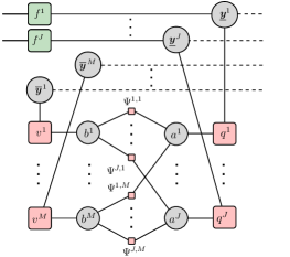
Figure 1: Factor graph representing the joint posterior pdf $f\big{(}\bm{x}_{0:k},\bm{r}_{0:k}$, $\bm{a}_{1:k},\bm{b}_{1:k}\big{|}\bm{z}_{1:k}\big{)}$ in (LABEL:eq:jointPosteriorComplete), (2) for one time step $k$. The time index $k$ is omitted, and the following short notations are used: $M\triangleq M_{k}$, $J\triangleq J_{k-1}$, $\underline{\bm{y}}^{j}\triangleq[\underline{\bm{x}}^{(j)\text{T}}_{k}\hskip 0.85358pt\underline{r}^{(j)}_{k}]^{\text{T}}$, $\overline{\bm{y}}^{m}\triangleq[\overline{\bm{x}}^{(m)\text{T}}_{k}\hskip 0.85358pt\overline{r}^{(m)}_{k}]^{\text{T}}$, $a^{j}\triangleq a^{(j)}_{k}$, $b^{m}\triangleq b^{(m)}_{k}$, $f^{j}\triangleq f\big{(}\underline{\bm{x}}^{(j)}_{k},\underline{r}^{(j)}_{k}\big{|}\bm{x}^{(j)}_{k-1},r^{(j)}_{k-1}\big{)}$, $q^{j}\triangleq q\big{(}\underline{\bm{x}}^{(j)}_{k},\underline{r}^{(j)}_{k},a_{k}^{(j)};\bm{z}_{k}\big{)}$, $v^{m}\triangleq v\big{(}\overline{\bm{x}}^{(m)}_{k},\overline{r}^{(m)}_{k},b_{k}^{(m)};\bm{z}^{(m)}_{k}\big{)}$, $\Psi^{j,m}\triangleq\Psi_{j,m}\big{(}a^{(j)}_{k},b^{(m)}_{k}\big{)}$.

Marginalizing out the redundant measurement-oriented DA vector $\bm{\mathsf{b}}_{1:k}$ from $f(\bm{x}_{0:k},\bm{r}_{0:k},\bm{a}_{1:k},\bm{b}_{1:k}|\bm{z}_{1:k})$ yields the posterior pdf

$$f(\bm{x}_{0:k},\bm{r}_{0:k},\bm{a}_{1:k}|\bm{z}_{1:k})=\sum_{\bm{b}_{1:k}}f(\bm{x}_{0:k},\bm{r}_{0:k},\bm{a}_{1:k},\bm{b}_{1:k}|\bm{z}_{1:k})\hskip 0.85358pt.$$

This marginalization is in fact trivial since for a given $\bm{a}_{1:k}$ there is exactly one $\bm{b}_{1:k}$ for which (LABEL:eq:jointPosteriorComplete) is nonzero. The posterior pdf $f(\bm{x}_{0:k},\bm{r}_{0:k},\bm{a}_{1:k}|\bm{z}_{1:k})$ in (LABEL:eq:jointPosteriorComplete1) together with expression (LABEL:eq:jointPosteriorComplete), (2) represents a system model that is identical to the one used by MHT methods and also is a generalization of the one used by JPDA filter methods.

III MHT Methods and Track Repulsion Effect

MHT methods aim at calculating the MAP sequence estimate of $\bm{\mathsf{x}}_{0:k}$, $\bm{\mathsf{r}}_{0:k}$, and $\bm{\mathsf{a}}_{1:k}$ from $\bm{z}_{1:k}$. This is done in two steps. First, the joint MAP sequence estimate of $\bm{\mathsf{r}}_{0:k}$ and $\bm{\mathsf{a}}_{1:k}$ is calculated, i.e.,

$$\big{(}\hat{\bm{r}}^{\text{MAP}}_{0:k}\!,\hat{\bm{a}}^{\text{MAP}}_{1:k}\big{)}=\hskip 0.85358pt\operatorname*{argmax}_{\bm{r}_{0:k},\hskip 0.85358pt\bm{a}_{1:k}}\int\!f(\bm{x}_{0:k},\bm{r}_{0:k},\bm{a}_{1:k}|\bm{z}_{1:k})\,\text{d}\bm{x}_{0:k}\hskip 0.85358pt.\!\!$$ (6)

This is equivalent to searching for the PT-measurement association $(\bm{r}_{0:k},\bm{a}_{1:k})$ that is most probable given the measurements $\bm{z}_{1:k}$ [7]. The marginalization operation $\int\cdot\,\text{d}\bm{x}_{0:k}$ can be performed sequentially and, assuming linear-Gaussian state-transition and measurement models, also in closed form. On the other hand, the number of PT-measurement associations $(\bm{r}_{0:k},\bm{a}_{1:k})$ that must be searched to perform the maximization (6) grows exponentially with $k$. In the second step, the MAP estimate of $\bm{\mathsf{x}}_{0:k}$ given $\bm{r}_{0:k}\!=\!\hat{\bm{r}}^{\text{MAP}}_{0:k}$ and $\bm{a}_{1:k}\!=\!\hat{\bm{a}}^{\text{MAP}}_{1:k}$ is calculated, i.e.,

$$\hat{\bm{x}}_{0:k}^{\text{MAP}} =\hskip 0.85358pt\operatorname*{argmax}_{\bm{x}_{0:k}}f\big{(}\bm{x}_{0:k}\big{|}\hat{\bm{r}}^{\text{MAP}}_{0:k}\!,\hat{\bm{a}}^{\text{MAP}}_{1:k}\!,\bm{z}_{1:k}\big{)}$$

$$=\hskip 0.85358pt\operatorname*{argmax}_{\bm{x}_{0:k}}f\big{(}\bm{x}_{0:k},\hat{\bm{r}}^{\text{MAP}}_{0:k}\!,\hat{\bm{a}}^{\text{MAP}}_{1:k}\big{|}\bm{z}_{1:k}\big{)}\hskip 0.85358pt.$$ (7)

Here, for $(\bm{r}_{0:k},\bm{a}_{1:k})=\big{(}\hat{\bm{r}}^{\text{MAP}}_{0:k}\!,\hat{\bm{a}}^{\text{MAP}}_{1:k}\big{)}$ fixed, the joint posterior $f\big{(}\bm{x}_{0:k},\hat{\bm{r}}^{\text{MAP}}_{0:k}\!,\hat{\bm{a}}^{\text{MAP}}_{1:k}\big{|}\bm{z}_{1:k}\big{)}$ in (LABEL:eq:jointPosteriorComplete1) factorizes into the posterior distributions $f\big{(}\bm{x}_{0:k}^{(j)},\hat{\bm{r}}^{(j)\text{MAP}}_{0:k}\!,\hat{\bm{a}}^{(j)\text{MAP}}_{1:k}\big{|}\bm{z}_{1:k}\big{)}$, one for each detected target $j$. The maximization (7) is then equivalent to a Bayesian smoothing operation—carried out by using, e.g., the Kalman smoother—for each detected target $j$ in parallel with, and independently of, all the other detected targets.

In a practical implementation, to reduce the computational complexity, the MAP estimates of the PT-measurement association sequence in (6) and of the kinematic PT state sequence in (7) are computed only over a sliding window of $N$ consecutive times steps. A hard decision on the PT-measurement association is made only at the oldest step within the window.

MHT can be formulated in a hypothesis-oriented [7] and track-oriented [23, 24, 25] manner. The two formulations are equivalent under the assumption that target births and clutter follow Poisson point processes [50]; however, the track-oriented MHT formulation offers a more compact representation of the DA problem. The computational complexity of the original hypothesis-oriented MHT formulation is still problematic due to the high number of hypotheses. However, it can be reduced by discarding unlikely hypotheses using, e.g., an efficient $m$-best assignment algorithm [21, 22]. The more efficient track-oriented MHT methods [23, 24, 25] represent the DA hypotheses by a set of tree structures, where each tree represents the possible DA histories of a single PT. The most likely hypothesis is then found by choosing a leaf node from each single-PT tree so that no measurement is used by more than one PT. A fast hypothesis search is enabled by combinatorial optimization methods [51, 26, 52, 53].

A limitation of MHT methods known as track repulsion can arise when targets come in close proximity. The estimated tracks then tend to have a larger distance than the true tracks. This effect is a consequence of performing hard DA by considering for PT state estimation (see (7)) only the single PT-measurement association $\big{(}\hat{\bm{r}}^{\text{MAP}}_{0:k}\!,\hat{\bm{a}}^{\text{MAP}}_{1:k}\big{)}$ in (6). For an illustration, consider two targets that move on parallel tracks. We assume that the states of the targets consist of their positions and velocities; furthermore, each target generates one measurement, which is the target’s position plus Gaussian measurement noise. The detection probability is assumed to be one and there are no clutter measurements. The target tracks are supposed to be in close proximity, in the sense that their distance is significantly smaller than the standard deviation of the measurement noise. The MAP decision rule (6) now always assigns to each measurement the nearest target. However, due to the small distance between the two targets, this association is often incorrect because the measurement closest to a given target originated from the respective other target. A number of consecutive incorrect associations will then cause the position estimates in (7) to be more distant than the actual targets; this effect is known as track repulsion. The track repulsion effect gets worse as the distance between the targets decreases.

The track repulsion effect can increase the estimation error and lead to track swaps (or identity switches) [54, 55]. In particular, in a scenario with crossing tracks, the estimated tracks tend to “bounce” more often than they cross. A method for mitigating track repulsion was presented in [40].

IV JPDA Filter Methods and Track Coalescence
Effect

The JPDA filter aims to calculate the MMSE estimates of the kinematic target states $\bm{\mathsf{x}}_{k}^{(j)}$, i.e.,

$$\hat{\bm{x}}_{k}^{(j)\text{MMSE}}=\int\!\bm{x}^{(j)}_{k}f\big{(}\bm{x}^{(j)}_{k}\big{|}\bm{z}_{1:k}\big{)}\,\text{d}\bm{x}_{k}^{(j)},\quad j=1,\dots,L_{k}\hskip 0.85358pt.$$ (8)

Here, $L_{k}$ denotes the number of actual targets (not PTs) at time $k$. The posterior pdf of the joint state $\bm{\mathsf{x}}_{k}=\big{[}{\bm{\mathsf{x}}}^{(1)\text{T}}_{k}\cdots\hskip 0.85358pt{\bm{\mathsf{x}}}^{(L_{k})\text{T}}_{k}\big{]}^{\mathrm{T}}\!$ is given by

$$f(\bm{x}_{k}|\bm{z}_{1:k}) =\sum_{\bm{a}_{k}}\hskip 0.85358ptf(\bm{x}_{k},\bm{a}_{k}|\bm{z}_{1:k})$$

$$=\hskip 0.85358pt\sum_{\bm{a}_{k}}f(\bm{x}_{k}|\bm{a}_{k},\bm{z}_{1:k})\hskip 0.85358ptp(\bm{a}_{k}|\bm{z}_{1:k})\hskip 0.85358pt.$$ (9)

The JPDA filter is based on the approximation of the posterior DA pmf $p(\bm{a}_{k}|\bm{z}_{1:k})$ involved in (9) by the product of its marginals, i.e. [1, 5]

$$p(\bm{a}_{k}|\bm{z}_{1:k})\approx\prod_{j=1}^{L_{k}}p\big{(}a^{(j)}_{k}\big{|}\bm{z}_{1:k}\big{)}\hskip 0.85358pt,\vspace{-2mm}$$ (10)

with

$$p\big{(}a^{(j)}_{k}\big{|}\bm{z}_{1:k}\big{)}=\sum_{\bm{a}_{k}^{(\sim j)}}p(\bm{a}_{k}|\bm{z}_{1:k})\hskip 0.85358pt.\vspace{-1mm}$$ (11)

Here, $\bm{a}_{k}^{(\sim j)}$ denotes the vector $\bm{a}_{k}$ with the $j$th entry $a^{(j)}_{k}$ removed. The posterior DA pmf $p(\bm{a}_{k}|\bm{z}_{1:k})$ is given as [5]

$$p(\bm{a}_{k}|\bm{z}_{1:k})=\prod_{j=1}^{L_{k}}\beta_{k}^{(j,a_{k}^{(j)})}\hskip 0.85358pt,\vspace{-2mm}$$ (12)

with

$$\beta_{k}^{(j,a_{k}^{(j)})}=\int\hskip 0.85358ptq\big{(}\bm{x}^{(j)}_{k}\!,1,a^{(j)}_{k};\bm{z}_{k}\big{)}\hskip 0.85358ptf\big{(}\bm{x}_{k}^{(j)}\big{|}\bm{z}_{1:k-1}\big{)}\hskip 0.85358pt\text{d}\bm{x}_{k}^{(j)}\hskip 0.85358pt,\vspace{1mm}$$ (13)

for $j=1,\ldots,L_{k}$ and $a_{k}^{(j)}=0,\ldots,M_{k}$. Here, the function $q\big{(}\bm{x}^{(j)}_{k}\!,1,a^{(j)}_{k};\bm{z}_{k}\big{)}$ is given by (LABEL:eq:qFunction) with $\underline{\bm{x}}_{k}^{(j)}$ replaced by $\bm{x}_{k}^{(j)}$, and $f\big{(}\bm{x}_{k}^{(j)}\big{|}\bm{z}_{1:k-1}\big{)}$ is the “predicted” posterior pdf of $\bm{\mathsf{x}}_{k}^{(j)}$. Furthermore, based on the assumption that, for $a_{k}^{(j)}=m$, the measurements $\bm{\mathsf{z}}_{k}^{(m)}$ are conditionally independent given $\bm{x}_{k}^{(j)}$ of all past and future measurements $\bm{\mathsf{z}}_{k^{\prime}}^{(m)}$ and states $\bm{\mathsf{x}}_{k^{\prime}}^{(j)}$ with $k^{\prime}\neq k$, it is shown in [5] that the pdf $f(\bm{x}_{k}|\bm{a}_{k},\bm{z}_{1:k})$ involved in (9) factors as

$$f(\bm{x}_{k}|\bm{a}_{k},\bm{z}_{1:k})=\prod_{j=1}^{L_{k}}f\big{(}\bm{x}_{k}^{(j)}\big{|}a_{k}^{(j)},\bm{z}_{1:k}\big{)}\hskip 0.85358pt.$$ (14)

Then, by inserting (10) into (9) and using the factorization (14), we arrive at the approximate posterior pdf

$$f(\bm{x}_{k}|\bm{z}_{1:k})\hskip 0.85358pt \approx\sum_{\bm{a}_{k}}\prod_{j=1}^{L_{k}}f\big{(}\bm{x}_{k}^{(j)}\big{|}a_{k}^{(j)},\bm{z}_{1:k}\big{)}\hskip 0.85358ptp\big{(}a_{k}^{(j)}\big{|}\bm{z}_{1:k}\big{)}$$

$$=\prod_{j=1}^{L_{k}}\sum_{a_{k}^{(j)}=\hskip 0.85358pt0}^{M_{k}}\!f\big{(}\bm{x}_{k}^{(j)}\big{|}a_{k}^{(j)},\bm{z}_{1:k}\big{)}\hskip 0.85358ptp\big{(}a_{k}^{(j)}\big{|}\bm{z}_{1:k}\big{)}$$

$$=\prod_{j=1}^{L_{k}}\tilde{f}\big{(}\bm{x}_{k}^{(j)}\big{|}\bm{z}_{1:k}\big{)}\hskip 0.85358pt,$$ (15)

with

$$\tilde{f}\big{(}\bm{x}_{k}^{(j)}\big{|}\bm{z}_{1:k}\big{)}\triangleq\!\sum_{a_{k}^{(j)}=\hskip 0.85358pt0}^{M_{k}}\!f\big{(}\bm{x}_{k}^{(j)}\big{|}a_{k}^{(j)},\bm{z}_{1:k}\big{)}\hskip 0.85358ptp\big{(}a_{k}^{(j)}\big{|}\bm{z}_{1:k}\big{)}\hskip 0.85358pt.$$ (16)

Here, the conditional pdf $f\big{(}\bm{x}_{k}^{(j)}\big{|}a_{k}^{(j)},\bm{z}_{1:k}\big{)}$ is given as follows [5]: for $a_{k}^{(j)}\!=m\in\{1,\ldots,M_{k}\}$,

$$f\big{(}\bm{x}_{k}^{(j)}\big{|}a_{k}^{(j)}\!=m,\bm{z}_{1:k}\big{)}$$

$$=\frac{f\big{(}\bm{z}_{k}^{(m)}\big{|}\bm{x}_{k}^{(j)}\big{)}\hskip 0.85358ptf\big{(}\bm{x}_{k}^{(j)}\big{|}\bm{z}_{1:k-1}\big{)}}{\int f\big{(}\bm{z}_{k}^{(m)}\big{|}\bm{x}_{k}^{(j)^{\prime}}\big{)}\hskip 0.85358ptf\big{(}\bm{x}_{k}^{(j)^{\prime}}\big{|}\bm{z}_{1:k-1}\big{)}\hskip 0.85358pt\text{d}\bm{x}_{k}^{(j)^{\prime}}}\hskip 0.85358pt,\quad\!\!m\!\in\!\{1,\ldots,M_{k}\}\hskip 0.85358pt,$$

and for $a_{k}^{(j)}\!=0$,

$$f\big{(}\bm{x}_{k}^{(j)}\big{|}a_{k}^{(j)}\!=0,\bm{z}_{1:k}\big{)}=f\big{(}\bm{x}_{k}^{(j)}\big{|}\bm{z}_{1:k-1}\big{)}\hskip 0.85358pt.$$ (18)

We note that, based on the approximation (10), the pdfs $\tilde{f}\big{(}\bm{x}_{k}^{(j)}\big{|}\bm{z}_{1:k}\big{)}$ in (15) and (16) approximate the marginal posterior pdfs $f\big{(}\bm{x}_{k}^{(j)}\big{|}\bm{z}_{1:k}\big{)}$.

In conventional JPDA filter methods, differently from MHT methods, the sequence of existence indicators $\bm{r}_{0:k}$, and thus also the number of targets $L_{k}$, are assumed known. In practical implementations, a heuristic for track initialization and termination provides an estimate of $\bm{r}_{0:k}$. For linear and Gaussian measurement and motion models and a Gaussian prior for the kinematic states $\bm{\mathsf{x}}_{k}^{(j)}$, as assumed in the original formulation of the JPDA filter [6, 9, 1], the approximate marginal posteriors pdfs $\tilde{f}\big{(}\bm{x}^{(j)}_{k}\big{|}\bm{z}_{1:k}\big{)}$ in (16) are Gaussian mixture pdfs which are further approximated by Gaussian pdfs.

A deficiency of the JPDA filter is the track coalescence effect: when targets come close to each other, the estimated tracks tend to merge and become indistinguishable. This behavior is due to the facts that (i) the predicted marginal posterior distributions $f\big{(}\bm{x}_{k}^{(j)}\big{|}\bm{z}_{1:k-1}\big{)}$ involved in (LABEL:eq:JPDA_approx3) and (18) become similar when the targets come close to each other, and (ii) the approximate marginal posterior distributions $\tilde{f}\big{(}\bm{x}^{(j)}_{k}\big{|}\bm{z}_{1:k}\big{)}$ are calculated via expression (16). More specifically, performing “soft DA” by means of the summation over all possible associations $a_{k}^{(j)}\!\in\{0,1,\ldots,M_{k}\}$, as done in (16), has the effect that targets $j$ with similar predicted marginal posterior distributions $f\big{(}\bm{x}_{k}^{(j)}\big{|}\bm{z}_{1:k-1}\big{)}$—which enter (16) via (LABEL:eq:JPDA_approx3) and (18)—tend to have similar approximate marginal posterior distributions $\tilde{f}\big{(}\bm{x}^{(j)}_{k}\big{|}\bm{z}_{1:k}\big{)}$. This, in turn, results in similar MMSE state estimates according to (8) (with $f\big{(}\bm{x}^{(j)}_{k}\big{|}\bm{z}_{1:k}\big{)}$ replaced by $\tilde{f}\big{(}\bm{x}^{(j)}_{k}\big{|}\bm{z}_{1:k}\big{)}$). A more detailed analysis of the track coalescence effect will be presented in Section VI.

Variants and extensions of the JPDA filter include the JIPDA filter [16, 2], the JPDA* filter [38], and the set JPDA (SJPDA) filter [41]. The JIPDA filter extends the JPDA filter by a binary existence indicator to systematically account for target existence, but suffers from track coalescence just as the conventional JPDA filter. The JPDA* filter mitigates track coalescence by pruning target-measurement associations. However, this comes at the cost of a reduced tracking performance in more challenging tracking scenarios with a high number of clutter measurements and missed detections. The SJPDA filter is based on the optimal subpattern assignment (OSPA) estimator [41], which is in turn based on the minimization of the mean OSPA metric [56]. Similar to the JPDA* filter, the SJPDA filter exhibits reduced coalescence effects. Efficient implementations are based on convex optimization techniques [57]. To maintain track continuity, the SJPDA filter relies on post-processing techniques [58], which are not required for the other JPDA filter variants or MHT tracking methods.

A potential limitation of the JPDA filter and its variants is the fact that their complexity scales exponentially with the number of targets and the number of measurements, which is due to the marginalization operation in (11) or equivalent marginalization operations. Gating and clustering strategies can significantly reduce the complexity in many cases, but fail when many objects come in close proximity. A potential solution in such scenarios is to switch to tracking methods of lower complexity such as the methods proposed in [59, 18]. Other solutions rely on the pruning of target-measurement associations—which is inherently done in the JPDA* filter—or exploit the potential independence of target-measurement associations [19].

V BP Methods

BP-based MTT methods [46, 5, 60, 15, 12, 34, 61] aim at computing the marginal posterior pdf $f\big{(}\bm{x}^{(j)}_{k},r^{(j)}_{k}\big{|}\bm{z}_{1:k}\big{)}$ for each PT $j\in\{1,\dots,J_{k}\}$. This marginal posterior pdf is then used to perform target detection and MMSE state estimation. In what follows, we will consider the specific BP method introduced in [5]. For target detection, within the BP method, the marginal posterior pmf $p\big{(}r^{(j)}_{k}\big{|}\bm{z}_{1:k}\big{)}$ of the existence indicator $\mathsf{r}^{(j)}_{k}$ is obtained from $f\big{(}\bm{x}^{(j)}_{k},r^{(j)}_{k}\big{|}\bm{z}_{1:k}\big{)}$ as

$$p\big{(}r^{(j)}_{k}\big{|}\bm{z}_{1:k}\big{)}=\int f\big{(}\bm{x}^{(j)}_{k},r^{(j)}_{k}\big{|}\bm{z}_{1:k}\big{)}\hskip 0.85358pt\mathrm{d}\bm{x}^{(j)}_{k}.\vspace{-1mm}$$ (19)

PT $j$ is then detected—i.e., declared to exist—if $p\big{(}r^{(j)}_{k}\!=\!1\big{|}\bm{z}_{1:k})$ is larger than a predefined threshold $P_{\text{th}}$. Next, for all PTs that are declared to exist, MMSE state estimation is performed according to

$$\hat{\bm{x}}^{(j)\text{MMSE}}_{k}\hskip 0.85358pt=\int\bm{x}^{(j)}_{k}f\big{(}\bm{x}^{(j)}_{k}\big{|}r^{(j)}_{k}\!=\!1,\bm{z}_{1:k}\big{)}\hskip 0.85358pt\mathrm{d}\bm{x}^{(j)}_{k},\vspace{-.5mm}$$ (20)

with

$$f\big{(}\bm{x}^{(j)}_{k}\big{|}r^{(j)}_{k}\!=\!1,\bm{z}_{1:k}\big{)}=\frac{f\big{(}\bm{x}^{(j)}_{k},r^{(j)}_{k}\!=\!1\big{|}\bm{z}_{1:k}\big{)}}{p\big{(}r^{(j)}_{k}\!=\!1\big{|}\bm{z}_{1:k}\big{)}}\hskip 0.85358pt.$$ (21)

It remains to calculate $f\big{(}\bm{x}^{(j)}_{k},r^{(j)}_{k}\big{|}\bm{z}_{1:k}\big{)}$. We have

$$f\big{(}\bm{x}^{(j)}_{k},r^{(j)}_{k}\big{|}\bm{z}_{1:k}\big{)}=\int\!\sum_{\bm{r}^{(\sim j)}_{k}}f(\bm{x}_{k},\bm{r}_{k}|\bm{z}_{1:k})\hskip 0.85358pt\mathrm{d}\bm{x}^{(\sim j)}_{k},\vspace{-1.5mm}$$

where $\bm{r}^{(\sim j)}_{k}$ denotes $\bm{r}_{k}$ with the entry ${r}^{(j)}_{k}$ removed, $\bm{x}^{(\sim j)}_{k}$ denotes $\bm{x}_{k}$ with the subvector $\bm{x}^{(j)}_{k}$ removed, and $f(\bm{x}_{k},\bm{r}_{k}|\bm{z}_{1:k})$ is a marginal pdf of the joint posterior pdf $f(\bm{x}_{0:k},\bm{r}_{0:k},\bm{a}_{1:k},\bm{b}_{1:k}|\bm{z}_{1:k})$, i.e.,

$$f(\bm{x}_{k},\bm{r}_{k}|\bm{z}_{1:k})$$

$$=\int\!\!\sum_{\bm{r}_{0:k-1}}\sum_{\bm{a}_{1:k}}\hskip 0.85358pt\sum_{\bm{b}_{1:k}}\hskip 0.85358ptf(\bm{x}_{0:k},\bm{r}_{0:k},\bm{a}_{1:k},\bm{b}_{1:k}|\bm{z}_{1:k})\,\mathrm{d}\bm{x}_{0:k-1}\hskip 0.85358pt.\!\!$$ (22)

By inserting the factorization (LABEL:eq:jointPosteriorComplete), (2) of $f(\bm{x}_{0:k},\bm{r}_{0:k},\bm{a}_{1:k},\linebreak\bm{b}_{1:k}|\bm{z}_{1:k})$ and carrying out the marginalizations with respect to $\bm{x}_{0:k-2}$, $\bm{r}_{0:k-2}$, $\bm{a}_{1:k-1}$, and $\bm{b}_{1:k-1}$, it can be shown that [5]

$$f(\bm{x}_{k},\bm{r}_{k}|\bm{z}_{1:k}) =\int\sum_{\bm{r}_{k-1}}\sum_{\bm{a}_{k}}\sum_{\bm{b}_{k}}f(\bm{x}_{k-1},\bm{r}_{k-1}|\bm{z}_{1:k-1})$$

$$\hskip 11.38109pt\times g(\bm{x}_{k},\bm{r}_{k},\bm{a}_{k},\bm{b}_{k},\bm{x}_{k-1},\bm{r}_{k-1};\bm{z}_{k})\hskip 0.85358pt\hskip 0.85358pt\mathrm{d}\bm{x}_{k-1},$$

where $g(\bm{x}_{k},\bm{r}_{k},\bm{a}_{k},\bm{b}_{k},\bm{x}_{k-1},\bm{r}_{k-1};\bm{z}_{k})$ was defined in (2).

Two observations can be made at this point. First, it can be concluded from (20)–(LABEL:eq:marginalization2) that the MMSE estimator $\hat{\bm{x}}^{(j)\text{MMSE}}_{k}$ in (20) is a “single-scan solution” in the sense that, as shown by (LABEL:eq:marginalization2), the marginal posterior pdf $f(\bm{x}_{k},\bm{r}_{k}|\bm{z}_{1:k})$ at time $k$ can be directly obtained from the marginal posterior pdf at time $k\!-\!1$,$f(\bm{x}_{k-1},\bm{r}_{k-1}|\bm{z}_{1:k-1})$, and the current measurement $\bm{z}_{k}$ (which enters via $g(\bm{x}_{k},\bm{r}_{k},\bm{a}_{k},\bm{b}_{k},\bm{x}_{k-1},\bm{r}_{k-1};\bm{z}_{k})$). In other words, $f(\bm{x}_{k-1},\bm{r}_{k-1}|\bm{z}_{1:k-1})$ subsumes and provides all the relevant information from past time steps. We note that a single-scan method based on MMSE estimation does not necessarily perform worse than a multiscan method based on MAP estimation (such as an MHT method).

Second, the computational complexity of evaluating the expressions (LABEL:eq:marginalization2) and (2) is much smaller than that of directly performing the marginalization in (22). Indeed, the summation over $\bm{r}_{0:k-1}$ in (22) involves $2^{J_{0}}\cdots 2^{J_{k-1}}=2^{\hskip 0.28453pt\sum^{k-1}_{k^{\prime}=0}J_{k^{\prime}}}$ terms, whereas the repeated application of (LABEL:eq:marginalization2) from $0$ to $k-1$ only involves $\sum^{k-1}_{k^{\prime}=0}\hskip 0.85358pt2^{\hskip 0.28453ptJ_{k^{\prime}}}$ terms. This complexity reduction is a consequence of the temporal factorization structure of the MTT problem. However, we still have to perform the marginalizations in (LABEL:eq:marginalization2), whose complexity scales exponentially in the number of targets and the number of measurements. These marginalizations can be computed in an efficient (though approximate) manner using the BP approach described in the following, which has only a linear complexity scaling.

The BP method operates on a factor graph representing the statistical model of the considered estimation problem [49, 48]. The factor graph for our statistical model is shown in Fig. 1. The marginal pdfs $f\big{(}\bm{x}^{(j)}_{k},\bm{r}^{(j)}_{k}\big{|}\bm{z}_{1:k}\big{)}$, $j=1,\dots,J_{k}$ needed for target detection and state estimation as discussed above are calculated efficiently by performing local operations corresponding to the individual graph nodes and exchanging the results of these local operations—called “messages”—along the graph edges [46, 5]. The BP approach systematically exploits the conditional independence structure of the involved random variables, as expressed by the factorization structure of (LABEL:eq:jointPosteriorComplete), (2) and represented by the factor graph of Fig. 1, for a large reduction of computational complexity. Here, in particular, the spatial factorization structure across PTs expressed by (LABEL:eq:jointPosteriorComplete) and (2) is exploited in addition to the temporal factorization structure. Since the factor graph in Fig. 1 has cycles, BP only provides approximations to the marginal pdfs $f\big{(}\bm{x}^{(j)}_{k},\bm{r}^{(j)}_{k}\big{|}\bm{z}_{1:k}\big{)}$ [49], which are referred to as “beliefs.” In the case of our factor graph, these beliefs are sufficiently accurate to yield excellent tracking performance. However, the cycles in the factor graph also lead to overconfident beliefs [62], i.e., the spread of the beliefs underestimates the true posterior uncertainty of the respective random variables.

Since the BP method performs a marginalization similar to JPDA filter methods, one may suspect that it suffers from track coalescence to a similar extent. Surprisingly, this is not the case: as analyzed in the next section and further evidenced by our simulation results in Section VII, the BP method exhibits track coalescence to a lesser extent than traditional JPDA filtering methods. Moreover, since the BP method performs state estimation in a way that is similar to JPDA filter methods, it does not suffer from track repulsion effects.

VI A Closer Look at the Track Coalescence Effect

In this section, we take a closer look at the track coalescence effect and investigate why BP methods exhibit this effect to a lesser extent than JPDA filter methods.

VI-A JPDA Filter

Let us first reconsider the JPDA filter from Section IV for the case where the number of targets is fixed and known, i.e., $L_{k}=L$ for all times $k$. It can here be shown that the joint posterior DA pmf $p(\bm{a}_{k}|\bm{z}_{1:k})$ can be expressed as

$$p(\bm{a}_{k}|\bm{z}_{1:k}) \propto\int\!\Psi(\bm{a}_{k})\hskip 0.85358pt\bigg{(}\prod^{L}_{j=1}q\big{(}\bm{x}^{(j)}_{k}\!,1,a^{(j)}_{k};\bm{z}_{k}\big{)}$$

$$\hskip 71.13188pt\times f\big{(}\bm{x}^{(j)}_{k}\big{|}\bm{z}_{1:k-1}\big{)}\bigg{)}\hskip 0.85358pt\mathrm{d}\bm{x}_{k}\hskip 0.85358pt,$$ (24)

where $\Psi(\bm{a}_{k})\triangleq\sum_{\bm{b}_{k}}\prod^{L}_{j=1}\prod^{M_{k}}_{m=1}\!\Psi_{j,m}\big{(}a_{k}^{(j)},b_{k}^{(m)}\big{)}$, with $\Psi_{j,m}\big{(}a_{k}^{(j)},b_{k}^{(m)}\big{)}$ as defined in Section II-C, is an indicator function that ensures that $\bm{a}_{k}$ satisfies the DA assumption. It can easily be verified that if $f\big{(}\bm{x}^{(j)}_{k}\big{|}\bm{z}_{1:k-1}\big{)}$, i.e., the “prior information” about $\bm{\mathsf{x}}^{(j)}_{k}$ at time $k$, is equal for all $j=1,\dots,L$, then $f\big{(}\bm{x}_{k}^{(j)}\big{|}a_{k}^{(j)},\bm{z}_{1:k}\big{)}$ in (LABEL:eq:JPDA_approx3), (18) is also equal for all $a_{k}^{(j)}=0,\ldots,M_{k}$. Furthermore, $p(\bm{a}_{k}|\bm{z}_{1:k})$ is invariant to a permutation of the entries $a^{(j)}_{k}$ of $\bm{a}_{k}$. This, in turn, implies that the marginal posterior DA pmfs $p\big{(}a^{(j)}_{k}\big{|}\bm{z}_{1:k}\big{)}$, $j=1,\dots,L$ calculated from $p(\bm{a}_{k}|\bm{z}_{1:k})$ according to (11) are equal and, further, the approximate marginal state pdfs $\tilde{f}\big{(}\bm{x}_{k}^{(j)}\big{|}\bm{z}_{1:k}\big{)}$, $j=1,\dots,L$ calculated from $p\big{(}a_{k}^{(j)}\big{|}\bm{z}_{1:k}\big{)}$ and $f\big{(}\bm{x}_{k}^{(j)}\big{|}a_{k}^{(j)},\bm{z}_{1:k}\big{)}$ according to (16) are equal as well. Therefore, the target state estimates $\bm{x}^{(j)\text{MMSE}}_{k}$ calculated from $\tilde{f}\big{(}\bm{x}_{k}^{(j)}\big{|}\bm{z}_{1:k}\big{)}$ according to (8) (with $f\big{(}\bm{x}^{(j)}_{k}\big{|}\bm{z}_{1:k}\big{)}$ replaced by $\tilde{f}\big{(}\bm{x}_{k}^{(j)}\big{|}\bm{z}_{1:k}\big{)}$) become equal, which means that the estimated tracks merge and, thus, the track coalescence effect is observed. An inspection of (16) and (24) shows that this indistinguishability of targets with the same prior information $f\big{(}\bm{x}^{(j)}_{k}\big{|}\bm{z}_{1:k-1}\big{)}$ is a direct consequence of the measurement model with measurement-origin uncertainty. We will illustrate this fact by considering two simple scenarios.

The first scenario demonstrates the track coalescence effect without using the Gaussian assumption underlying the JPDA filter. We consider a one-dimensional state space and two targets that are close to each other. The target states are the targets’ one-dimensional positions $x_{k}^{(j)}\in\{-1,1\}$ for $j\!=\!1,2$. The targets are observed by a sensor that generates the measurements $z_{k}^{(1)}\!=\!1$ and $z_{k}^{(2)}\!=-1$. Thus, we have $L_{k}=L=2$ and $M_{k}=2$. There are no clutter measurements and no measurement noise, and the detection probability is assumed to be one. We further assume that each measurement equals either one of the true target positions $x_{k}^{(j)}$ with equal probability, i.e., $z_{k}^{(1)}\!=\!1$ equals $x_{k}^{(1)}$ or $x_{k}^{(2)}$ with equal probability $1/2$, and similarly for $z_{k}^{(2)}\!=-1$. It can be shown that this results in equal marginal association probabilities $p\big{(}a_{k}^{(1)}=m\big{|}\bm{z}_{1:k}\big{)}=p\big{(}a_{k}^{(2)}=m\big{|}\bm{z}_{1:k}\big{)}=1/2$ for $m=1,2$. It can furthermore be shown that this results in approximate marginal posterior pdfs, according to (16), that are given by $\tilde{f}\big{(}x_{k}^{(j)}\big{|}\bm{z}_{1:k}\big{)}=\frac{1}{2}\hskip 0.85358pt\delta\big{(}x_{k}^{(j)}\!-\!1\big{)}+\frac{1}{2}\hskip 0.85358pt\delta\big{(}x_{k}^{(j)}\!+\!1\big{)}$ for $j\!=\!1,2$. Finally, using (8), the MMSE state estimates are obtained as $\hat{x}_{k}^{(j)\text{MMSE}}\!=0$ for $j\!=\!1,2$. This means that the tracks are merged and, thus, the track coalescence effect is observed.

In the second scenario, we reconsider the simple tracking scenario previously considered in the context of MHT methods in Section III. We recall this scenario for convenience. There are two targets, whose states consist of the targets’ positions and velocities. Each target generates one measurement, which is the target’s position plus Gaussian measurement noise, and there are no clutter measurements. Thus, we again have $L_{k}=L=2$ and $M_{k}=2$. The targets move on parallel tracks and in close proximity, in the sense that their distance is significantly smaller than the standard deviation of the measurement noise. If the two targets move in this way for a sufficiently long time, it can be expected that the predicted posterior pdfs $f\big{(}\bm{x}_{k}^{(1)}\big{|}\bm{z}_{1:k-1}\big{)}$ and $f\big{(}\bm{x}_{k}^{(2)}\big{|}\bm{z}_{1:k-1}\big{)}$, i.e., the “prior information,” are approximately equal and that each of the two measurements are approximately equally likely to have originated from either one of the two targets, which furthermore results in $f\big{(}\bm{x}_{k}^{(1)}\big{|}a_{k}^{(1)}\!=m,\bm{z}_{1:k}\big{)}$ and $f\big{(}\bm{x}_{k}^{(2)}\big{|}a_{k}^{(2)}\!=m,\bm{z}_{1:k}\big{)}$ in (LABEL:eq:JPDA_approx3) being approximately equal for $m=1,2$. As a consequence, it can be expected that, according to (11)–(13), $p\big{(}a_{k}^{(1)}\big{|}\bm{z}_{1:k}\big{)}$ and $p\big{(}a_{k}^{(2)}\big{|}\bm{z}_{1:k}\big{)}$ and, in turn, according to (16), $\tilde{f}\big{(}\bm{x}_{k}^{(1)}\big{|}\bm{z}_{1:k}\big{)}$ and $\tilde{f}\big{(}\bm{x}_{k}^{(2)}\big{|}\bm{z}_{1:k}\big{)}$ are almost equal. As explained above, this implies that the target state estimates $\bm{x}^{(1)\text{MMSE}}_{k}$ and $\bm{x}^{(2)\text{MMSE}}_{k}$ become approximately equal, which means that the track coalescence effect is observed. The track coalescence effect also occurs when one of the two targets is missed, i.e., $M_{k}\!=\!1$, or there is clutter, i.e., $M_{k}\!>\!2$, as long as the distance between the targets is smaller than the standard deviation of the measurement noise. In both cases, again, each of the measurements is approximately equally likely to have originated from either one of the two targets. If the measurements follow a more complicated, possibly nonlinear or non-Gaussian measurement model, the track coalescence effect can still be observed, but a characterization of the case where the targets are “in close proximity” is more difficult.

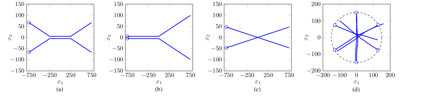
Figure 2: Target trajectories of scenarios (a) S1, (b) S2, (c) S3, and (d) S4. The initial target positions are indicated by circles.

VI-B BP Method

Although the BP method considered in Section V is partly related to the JPDA filtering paradigm, it exhibits significantly reduced track coalescence effects. There are two reasons for this fact: (i) the BP method typically uses a particle representation of the marginal posterior pdfs $f\big{(}\bm{x}^{(j)}_{k}\big{|}r^{(j)}_{k}\!=\!1,\bm{z}_{1:k}\big{)}$ in (21) [46], which preserves the multimodality of these pdfs, and (ii) the overconfident nature of the BP method favors the most likely PT-measurement association.

Reason (i) can be explained as follows. In the original JPDA filter, the pdfs $f\big{(}\bm{x}_{k}^{(j)}\big{|}a_{k}^{(j)},\bm{z}_{1:k}\big{)}$ in (LABEL:eq:JPDA_approx3) and (18) are Gaussian pdfs. As a consequence, the approximate marginal posterior pdfs $\tilde{f}\big{(}\bm{x}_{k}^{(j)}\big{|}\bm{z}_{1:k}\big{)}$ calculated according to (16) are Gaussian mixture pdfs. The JPDA filter approximates these multimodal Gaussian mixture pdfs by Gaussian pdfs. This additional approximation exacerbates the track coalescence effect since pdfs $\tilde{f}\big{(}\bm{x}_{k}^{(j)}\big{|}\bm{z}_{1:k}\big{)}$ that are well distinguishable may become indistinguishable after the Gaussian approximation. By contrast, the particle representation of the marginal posterior pdfs $f\big{(}\bm{x}^{(j)}_{k}\big{|}r^{(j)}_{k}\!=\!1,\bm{z}_{1:k}\big{)}$ that is used in the BP method is able to capture the multimodality of $f\big{(}\bm{x}^{(j)}_{k}\big{|}r^{(j)}_{k}\!=\!1,\bm{z}_{1:k}\big{)}$. We note that the role of $f\big{(}\bm{x}^{(j)}_{k}\big{|}r^{(j)}_{k}\!=\!1,\bm{z}_{1:k}\big{)}$ in the BP method is similar to that of $f\big{(}\bm{x}^{(j)}_{k}\big{|}\bm{z}_{1:k}\big{)}$ in JPDA filter methods.

Reason (ii) is the overconfident nature of the BP method for a factor graph with cycles (“loopy BP”) [63]. To illustrate this aspect, we consider modified marginal posterior DA pmfs $p_{\rho}\big{(}a^{(j)}_{k}\big{|}\bm{z}_{1:k}\big{)}\triangleq\big{(}p\big{(}a^{(j)}_{k}\big{|}\bm{z}_{1:k}\big{)}\big{)}^{\rho}/\hskip 0.85358ptC^{(j)}_{k}$ with exponent $\rho\in(0,\infty)$, where $C^{(j)}_{k}\triangleq\sum^{M_{k}}_{a^{(j)}_{k}\!=\hskip 0.85358pt0}\big{(}p\big{(}a^{(j)}_{k}\big{|}\bm{z}_{1:k}\big{)}\big{)}^{\rho}$ and $p\big{(}a^{(j)}_{k}\big{|}\bm{z}_{1:k}\big{)}$ is calculated according to (11). For $0<\rho<1$, $p_{\rho}\big{(}a^{(j)}_{k}\big{|}\bm{z}_{1:k}\big{)}$ is underconfident relative to $p\big{(}a^{(j)}_{k}\big{|}\bm{z}_{1:k}\big{)}$, in the sense that likely PT-measurement associations (corresponding to large values of $p\big{(}a^{(j)}_{k}\big{|}\bm{z}_{1:k}\big{)}$) are deemphasized and unlikely ones (corresponding to small values of $p\big{(}a^{(j)}_{k}\big{|}\bm{z}_{1:k}\big{)}$) are emphasized, resulting in a larger spread of the modified pmf $p_{\rho}\big{(}a^{(j)}_{k}\big{|}\bm{z}_{1:k}\big{)}$. In particular, for $\rho\rightarrow 0$, $p_{\rho}\big{(}a^{(j)}_{k}\big{|}\bm{z}_{1:k}\big{)}$ is the uniform pmf, i.e., all PT-measurement associations are equally likely. For $\rho>1$, on the other hand, $p_{\rho}\big{(}a^{(j)}_{k}\big{|}\bm{z}_{1:k}\big{)}$ is overconfident relative to $p\big{(}a^{(j)}_{k}\big{|}\bm{z}_{1:k}\big{)}$, in the sense that likely associations are emphasized and unlikely ones are deemphasized, resulting in a smaller spread of $p_{\rho}\big{(}a^{(j)}_{k}\big{|}\bm{z}_{1:k}\big{)}$. In particular, for $\rho\rightarrow\infty$, $p_{\rho}\big{(}a^{(j)}_{k}\big{|}\bm{z}_{1:k}\big{)}$ is one for the value of $a^{(j)}_{k}$ where $p\big{(}a^{(j)}_{k}\big{|}\bm{z}_{1:k}\big{)}$ is largest—i.e., the MAP estimate of $\mathsf{a}^{(j)}_{k}$—and zero otherwise. The JPDA filter performs soft DA with $\rho\!=\!1$, which leads to track coalescence as discussed above. By contrast, MHT methods perform hard DA, in that they use only the MAP estimate of $\mathsf{a}^{(j)}_{k}$ instead of the entire posterior distribution of $\mathsf{a}^{(j)}_{k}$, corresponding to $p_{\rho}\big{(}a^{(j)}_{k}\big{|}\bm{z}_{1:k}\big{)}$ with $\rho\rightarrow\infty$; this leads to track repulsion as explained in Section III.

The BP method, just as JPDA filtering methods, performs soft DA in the sense that it calculates approximate marginal posterior state pdfs $\tilde{f}\big{(}\bm{x}_{k}^{(j)}\big{|}\bm{z}_{1:k}\big{)}$ via a summation over all the possible associations, thereby taking into account the entire DA distribution (see (16)). However, in contrast to JPDA filter methods, it relies on loopy BP and thus computes overconfident approximations $\tilde{p}\big{(}a^{(j)}_{k}\big{|}\bm{z}_{1:k}\big{)}$ of the marginal posterior DA pmfs $p\big{(}a^{(j)}_{k}\big{|}\bm{z}_{1:k}\big{)}$. These approximations resemble $p_{\rho}\big{(}a^{(j)}_{k}\big{|}\bm{z}_{1:k}\big{)}$ with $\rho\!>\!1$, which means that the BP method emphasizes likely PT-measurement associations and deemphasizes unlikely ones. Thus, the soft DA performed by the BP method is somewhat closer, in regard to the tracking results, to the hard DA performed by MHT methods (which do not exhibit the track coalescence effect). This explains why the BP method exhibits a reduced track coalescence effect. Furthermore, since the BP method still performs soft DA similar to the JPDA filter, it does not exhibit a track repulsion effect.

VII Simulation Study

Next, we present simulation results assessing and comparing the performance of the considered MTT methods in four different scenarios where targets come in close proximity. In particular, we will demonstrate experimentally that the BP method exhibits no track repulsion effect and a significantly reduced track coalescence effect compared to JPDA filter methods.

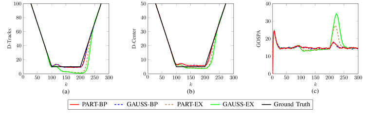
Figure 3: Performance of PART-BP, GAUSS-BP, PART-EX, and GAUSS-EX for scenario S1: (a) D-Tracks, (b) D-Center, and (c) GOSPA.

VII-A Simulation Setup

We consider the four simulation scenarios S1 through S4 depicted in Fig. 2. In S1, two targets approach each other, move in parallel close to each other, and separate again. In S2, two targets move in parallel close to each other from the beginning and then separate. In S3, two targets cross each other. In S4, six targets are born on a circle of radius 150 m; they move according to a nearly constant velocity motion model towards the origin, where they come in close proximity, and then separate again [46]. Each scenario comprises 300 time steps. The minimum distance between the two targets in S1 and S2 is equal to the standard deviation of the measurement noise, $\sigma_{\bm{v}}$ (defined below). The targets remain close to each other for 100 time steps in S1 and for 150 time steps in S2. In S3 and S4, the two and six targets are in a “2$\sigma_{\bm{v}}$-neighborhood” for about 50 time steps and 30 time steps, respectively. The region of interest (ROI) is $[-750\hskip 0.85358pt\text{m},\hskip 0.85358pt750\hskip 0.85358pt\text{m}]\times[-750\hskip 0.85358pt\text{m},\hskip 0.85358pt750\hskip 0.85358pt\text{m}]$ for all scenarios.

The target states consist of two-dimensional position and velocity, i.e., $\bm{\mathsf{x}}_{k}^{(j)}=\big{[}\mathsf{x}_{1,k}^{(j)}\;\hskip 0.85358pt\mathsf{x}_{2,k}^{(j)}\;\hskip 0.85358pt\dot{\mathsf{x}}_{1,k}^{(j)}\;\hskip 0.85358pt\dot{\mathsf{x}}_{2,k}^{(j)}\big{]}^{\text{T}}$. The various MTT methods use the nearly constant-velocity motion model [64]

$$\bm{\mathsf{x}}_{k}^{(j)}=\bm{A}\hskip 0.85358pt\bm{\mathsf{x}}^{(j)}_{k-1}+\bm{\mathsf{u}}_{k}^{(j)}\hskip 0.85358pt,$$

where $\bm{\mathsf{u}}_{k}^{(j)}\!\sim\!\mathcal{N}(\bm{0},\bm{\Sigma}_{\bm{u}})$ is a sequence of independent and identically distributed (iid) four-dimensional Gaussian random vectors and $\bm{A}$ and $\bm{\Sigma}_{\bm{u}}$ are given by

$$\small\bm{A}={\begin{pmatrix}1&0&T&0\\ 0&1&0&T\\ 0&0&1&0\\ 0&0&0&1\end{pmatrix}}\hskip 0.85358pt,\quad\,\bm{\Sigma}_{\bm{u}}={\begin{pmatrix}\frac{T^{3}}{3}&0&\frac{T^{2}}{2}&0\\ 0&\frac{T^{3}}{3}&0&\frac{T^{2}}{2}\\ \frac{T^{2}}{2}&0&T&0\\ 0&\frac{T^{2}}{2}&0&T\end{pmatrix}}\hskip 0.85358pt\sigma^{2}_{\bm{u}}\hskip 0.85358pt.\vspace{0mm}$$

Here, $T=1\hskip 0.85358pt\text{s}$ and $\sigma^{2}_{\bm{u}}\!=0.1\hskip 0.85358pt\hskip 0.85358pt\text{m}^{2}/\text{s}^{4}$ for S1, S2, and S3 and $\sigma^{2}_{\bm{u}}\!=0.0001\hskip 0.85358pt\hskip 0.85358pt\text{m}^{2}/\text{s}^{4}$ for S4. The survival probability is set to $p_{\text{s}}=0.995$.

The sensor produces noisy measurements of the target positions. More specifically, the target-generated measurements are given by

$$\bm{\mathsf{z}}_{k}^{(m)}=\hskip 0.85358pt[\mathsf{x}_{1,k}\;\hskip 0.85358pt\mathsf{x}_{2,k}]^{\text{T}}+\hskip 0.85358pt\bm{\mathsf{v}}_{k}^{(m)}\hskip 0.85358pt,\vspace{0mm}$$

where $\bm{\mathsf{v}}_{k}^{(m)}\!\sim\!\mathcal{N}(\bm{0},\sigma_{\bm{v}}^{2}{\bf I}_{2})$ with $\sigma_{\bm{v}}\!=\!10\,$m is an iid sequence of two-dimensional Gaussian random vectors. The detection probability is set to $p_{\text{d}}=0.5$. In addition to the target-generated measurements, there are also clutter measurements. The mean number of clutter measurements is $\mu_{\text{c}}\!=\!10$, and the clutter pdf $f_{\text{c}}\big{(}\bm{z}_{k}^{(m)}\big{)}$ is uniform on the ROI.

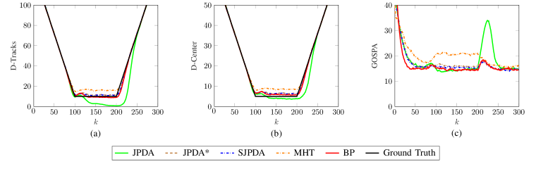
Figure 4: Performance of JPDA, JPDA*, SJPDA, MHT, and BP for scenario S1: (a) D-Tracks, (b) D-Center, and (c) GOSPA.

For each of our four scenarios, we performed 1000 Monte Carlo runs, each comprising 300 time steps. For performance evaluation, we use the general optimal subpattern assignment (GOSPA) metric [65] based on the L2-norm, averaged over all simulation runs, with parameters $p=1$, $c=50$, and $\beta=2$. The GOSPA metric accounts for both cardinality and state estimation errors, similar to the OSPA metric [56] and the complete OSPA metric [66]. For S1, we compute two additional performance metrics. The first, termed “D-Tracks,” is the distance between the two tracks, i.e., $|\hat{x}_{2,k}^{(1)}-\hat{x}_{2,k}^{(2)}|$, for each time step $k$. The second, termed “D-Center,” is the average of the distances of the estimated y-coordinates of the two tracks from the y-center (origin), i.e., $(|\hat{x}_{2,k}^{(1)}|+|\hat{x}_{2,k}^{(2)}|)/2$, again for each time step $k$. A small small D-Tracks metric can indicate track coalescence, while the D-Center metric assesses the accuracy of the tracks’ centroid (which is high if the D-Center metric is small). For example, if D-Tracks and D-Center are both zero, the estimated tracks may have coalesced, but at least the estimated “joint track” is quite accurate. On the other hand, if D-Center is large, then also the estimated joint track is inaccurate.

VII-B Reduced Track Coalescence in the BP Method

We first demonstrate and analyze experimentally the reduction of track coalescence exhibited by the BP method of Section V. In Section VI-B, we argued that this reduction is due to the particle representation of the marginal posterior state pdfs and the overconfident nature of the BP method. To demonstrate the influence of the particle representation of the marginal posterior state pdfs, we compare a particle implementation of the BP method with a Gaussian implementation; these implementations will be designated as PART-BP and GAUSS-BP, respectively. Furthermore, to demonstrate the influence of the overconfident nature of the BP method, we consider modified versions of the particle and Gaussian implementations in which the BP-based approximate marginalization of the association pmf is replaced by an exact marginalization. These latter methods will be designated as PART-EX and GAUSS-EX. To exclude the influence of target detection errors, we temporarily assume that the birth times and birth positions of the targets are perfectly known by the various tracking algorithms. Note that in this case GAUSS-EX coincides with the JPDA filter of Section IV. PART-BP and PART-EX use 5000 particles to represent the PT states. The threshold for target confirmation is $P_{\text{th}}=0.5$.

Fig. 3 presents the results for scenario S1. The D-Tracks curves in Fig. 3(a) show that the tracks of GAUSS-BP and PART-BP are close to the ground truth, whereas those of GAUSS-EX and PART-EX tend to merge and exhibit a delay in separating again. This behavior is also reflected by the GOSPA curves in Fig. 3(c): the coalescence effect causes an increase of the GOSPA error of GAUSS-EX and PART-EX for $k=200,\ldots,250$; this increase is smaller for PART-EX than for GAUSS-EX. Regarding the D-Center curves in Fig. 3(b), all four methods exhibit a similar behavior. In summary, the results in Figs. 3(a) and (c) demonstrate that the combination of particle representation and BP-based marginalization results in reduced track coalescence effects, thereby confirming our reasoning of Section VI.

VII-C Analysis of Track Coalescence and Repulsion for the
JPDA, JPDA*, SJPDA, MHT, and BP Methods

Next, we analyze the track coalescence and repulsion effects potentially exhibited by the JPDA, JPDA*, SJPDA, (track-oriented) MHT, and BP methods for our four scenarios S1 through S4. The number of targets and the target birth times and positions are now unknown to all methods. JPDA, JPDA*, and SJPDA use gating with a gate validation threshold of 13.82, corresponding to an in-gate probability (i.e., the probability that a target-generated measurement is within the gate) of 0.999. We remark that a gate validation threshold of 9.21, corresponding to an in-gate probability of 0.99, led to similar results. MHT uses a hypothesis depth of five scans. The track confirmation logics of JPDA, JPDA*, and SJPDA are set to 12/24, those of MHT to 8/16 (these values were chosen such that each method achieves its best performance across all scenarios). Finally, BP generates a new track for each measurement, sets the corresponding existence probability to $10^{-4}$, and prunes existing tracks with existence probabilities below $10^{-4}$.

Fig. 4 shows the D-Tracks, D-Center, and GOSPA curves for scenario S1. One can see in Fig. 4(a) that when the two targets move in close proximity, D-Tracks is increased for MHT and decreased for JPDA compared to the ground truth tracks; this indicates track repulsion and track coalescence, respectively. The low D-Tracks curve of JPDA for $k=200,\ldots,250$ demonstrates that, after they coalesced, the tracks estimated by JPDA separate again only with a delay. In JPDA*, SJPDA, and BP, track coalescence is strongly reduced. In the case of JPDA* and SJPDA, this is due to the special design of these methods; in the case of BP, it is due to the particle representation of the marginal posterior state pdfs and the overconfident nature of the BP method as argued in Section VI-B and verified experimentally in Section VII-B. Furthermore, in Fig. 4(b), the D-Center curves of JPDA, JPDA*, SJPDA, and BP are generally close to the true curves. An exception is JPDA for $k=200,\ldots,240$, which again reflects the fact that, after coalescence, the tracks estimated by JPDA separate again only with a delay. The GOSPA curves shown in Fig. 4(c) confirm the results of Figs. 4(a) and (b). In particular, the increased GOSPA error of MHT for $k=100,\ldots,200$ is due to track repulsion, and that of JPDA for $k=200,\ldots,250$ to track coalescence. JPDA*, SJPDA, and BP perform similarly well, with a slight performance advantage for BP.

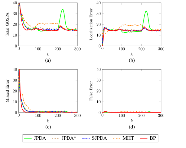
Figure 5: GOSPA error decomposition for scenario S1: (a) Total GOSPA error (same as Fig. 4(c)), (b) localization error component, (c) missed error component, and (d) false error component.

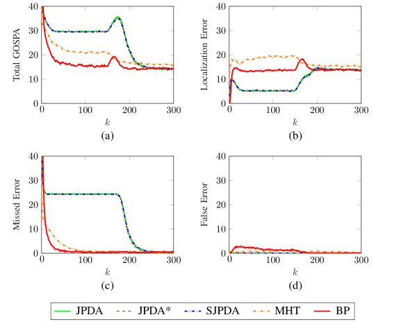
Figure 6: Total GOSPA error (a) and its components (b)–(d) for scenario S2.

Still for scenario S1, Figs. 5(b)–(d) show the individual GOSPA error components, i.e., the localization error, the error due to missed targets (“missed error”), and the error due to false targets (“false error”) [65]. In addition, the total GOSPA curves from Fig. 4(c) are replicated in Fig. 5(a) for easy reference. The localization error curves in Fig. 5(b) are seen to be similar to the total GOSPA curves; this reflects the fact that missed and false targets contribute only little to the total GOSPA error.

Fig. 6 shows the GOSPA error and its components for scenario S2. In S2, differently from S1, the two targets are in close proximity right from the beginning (see Fig. 2(b)). This poses a challenge for the track initiation stage of the JPDA filter methods. Indeed, JPDA, JPDA*, and SJPDA generate only one track as long as the targets remain in close proximity. This means that one of the targets is missed, resulting in a large missed error component of JPDA, JPDA*, and SJPDA in the time range $k=1,\ldots,200,$ as shown in Fig. 6(c). By contrast, as also shown in Fig. 6(c), MHT and BP initialize both tracks correctly. Fig. 6(b) indicates an increased localization error of MHT for $k=1,\ldots,150$; this is due to track repulsion as in S1. It is furthermore seen that the localization error of JPDA, JPDA*, and SJPDA is reduced; this can be explained by the fact that these methods estimate just a single track whereas the other methods estimate both tracks, combined with the fact that GOSPA is an “unnormalized” error metric, which implies that tracking fewer targets generally results in a lower localization error. Note, however, that the total GOSPA error is lowest for BP. Finally, Fig. 6(d) shows that the false error component is small for all methods.

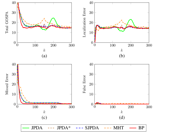
Figure 7: Total GOSPA error (a) and its components (b)–(d) for scenario S3.

Fig. 7 presents the GOSPA error and its components for scenario S3. Similarly to scenarios S1 and S2, it can be seen that when the two targets are close to each other, i.e., for $k=125,\ldots,175$, MHT suffers from track repulsion, and after the targets separate again, i.e., for $k=175,\ldots,225$, JPDA suffers from track coalescence. By contrast, track repulsion and track coalescence are nonexistent or significantly reduced in JPDA*, SJPDA, and BP.

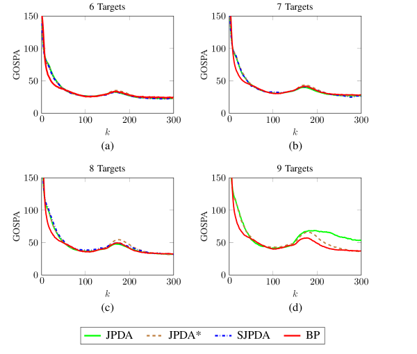
Figure 8: GOSPA error for scenario S4 (a) and for three variants of S4 with seven, eight, and nine targets (b)–(d).

VII-D Further Analysis of Track Coalescence for the
JPDA, JPDA*, SJPDA, and BP Methods

The results reported so far for scenarios S1 through S3 demonstrate that JPDA, JPDA*, SJPDA, and BP do not exhibit track repulsion and MHT does not exhibit track coalescence. In addition, JPDA*, SJPDA, and BP exhibit reduced track coalescence compared to conventional JPDA. Since JPDA*, SJPDA, and BP performed equally well, we now further analyze the track coalescence behavior of these methods and, for comparison, of conventional JPDA in the even more challenging scenario S4. Since MHT is not susceptible to track coalescence, it is not considered in this analysis. S4 features six targets, which come in close proximity around time $k\!=\!150$ (see Fig. 2(d)). We also consider more challenging variants of S4 with seven, eight, and nine targets. The GOSPA error for these scenarios is shown in Fig. 8. It can be seen that all four methods exhibit only small track coalescence effects for the cases of six, seven, and eight targets. For the case of nine targets, JPDA and JPDA* exhibit an increased GOSPA error compared to BP. In particular, the GOSPA error of JPDA remains high for a long time after the targets separate again.

		6 Targets	7 Targets	8 Targets	9 Targets
JPDA	min	0.54 s	0.90 s	2.05 s	18.76 s
	median	1.42 s	4.54 s	17.45 s	84.14 s
	mean	1.44 s	4.59 s	33.28 s	2952.90 s
	max	3.43 s	18.34 s	2758.00 s	9458.90 s
JPDA*	min	0.52 s	0.90 s	2.42 s	16.31 s
	median	1.22 s	4.89 s	34.66 s	256.08 s
	mean	1.29 s	5.35 s	39.70 s	309.18 s
	max	3.62 s	22.26 s	340.30 s	1653.30 s
SJPDA	min	1.28 s	16.21 s	132.57 s
	median	10.30 s	70.63 s	531.93 s
	mean	10.46 s	74.90 s	640.120 s
	max	36.73 s	251.72 s	4351.40 s
BP	min	18.62 s	19.33 s	21.03 s	21.76 s
	median	24.04 s	24.84 s	27.78 s	31.18 s
	mean	24.05 s	24.86 s	27.86 s	31.26 s
	max	28.44 s	29.88 s	31.80 s	36.48 s

TABLE I: Minimum, median, mean, and maximum runtimes of JPDA, JPDA*, SJPDA, and BP for scenario S4 (six targets) and its variants with seven, eight, and nine targets.

Still considering scenario S4 and its variants, we report in Table I the minimum, median, mean, and maximum total (for all 300 time steps) filter runtimes of Matlab implementations of JPDA, JPDA*, SJPDA, and BP on an Intel Xeon Gold 5222 CPU measured from 1000 Monte Carlo runs. Our JPDA, JPDA*, SJPDA, and BP implementations use gating and clustering to reduce computational complexity. However, in Scenario S4 and its variants, this has only a limited effect during the time the targets are in close proximity because the targets are within the same gate and thus clustered together. As Table I shows, the runtimes of JPDA, JPDA*, and SJPDA increase rapidly with the number of targets. This is consistent with the exponential scaling of the complexity of these filters in the number of tracks; note that the number of tracks may be higher than the number of targets because of false tracks that were generated due to clutter measurements. The exponential scaling also explains why JPDA and JDPA* are infeasible for more than nine targets and SJPDA for more than eight targets. Table I also shows that for JPDA, JPDA*, and SJPDA there is a large difference between the minimum and maximum filter runtime. The high filter runtimes are due to Monte Carlo runs where the number of tracks is higher than the actual number of targets. Because there are considerably more Monte Carlo runs with a low filter runtime than with a high filter runtime, the median runtimes differ significantly from the mean runtimes. On the other hand, the runtime of BP increases only slowly with the number of targets. This is consistent with the fact that the complexity of BP scales only linearly in the number of targets (tracks).

VIII Conclusion

We reviewed and analyzed three major methodologies for multitarget tracking: the classical joint probabilistic data association (JPDA) and multiple hypothesis tracking (MHT) methodologies and the recently introduced belief propagation (BP) methodology. The focus of our study was on track coalescence and track repulsion effects, which are well known to compromise the performance of, respectively, JPDA filter and MHT methods when targets are in close proximity. In particular, we investigated the potential occurrence of track coalescence and track repulsion effects in the BP method. We argued that the BP method does not suffer from track repulsion because it performs soft data association similarly to the JPDA filter. Moreover, track coalescence effects in the BP method are significantly smaller than in the JPDA filter, due to the use of a particle representation for multimodal distributions and the overconfident nature of the BP method. These theoretical arguments were confirmed by simulation experiments. Our numerical results demonstrated excellent performance of the BP method compared to the JPDA, JPDA*, set JPDA, and MHT methods in scenarios with targets in close proximity.

References

- [1] Y. Bar-Shalom, P. K. Willett, and X. Tian, Tracking and Data Fusion: A Handbook of Algorithms. Storrs, CT, USA: Yaakov Bar-Shalom, 2011.
- [2] S. Challa, M. R. Morelande, D. Mušicki, and R. J. Evans, Fundamentals of Object Tracking. Cambridge, UK: Cambridge University Press, 2011.
- [3] R. Mahler, Statistical Multisource-Multitarget Information Fusion. Norwood, MA, USA: Artech House, 2007.
- [4] W. Koch, Tracking and Sensor Data Fusion: Methodological Framework and Selected Applications. Berlin, Germany: Springer, 2014.
- [5] F. Meyer, T. Kropfreiter, J. L. Williams, R. Lau, F. Hlawatsch, P. Braca, and M. Z. Win, “Message passing algorithms for scalable multitarget tracking,” Proc. IEEE, vol. 106, no. 2, pp. 221–259, 2018.
- [6] Y. Bar-Shalom, “Extension of the probabilistic data association filter in multi-target tracking,” in Proc. SNETA-74, San Diego, CA, USA, Sep. 1974.
- [7] D. B. Reid, “An algorithm for tracking multiple targets,” IEEE Trans. Autom. Control, vol. 24, no. 6, pp. 843–854, Dec. 1979.
- [8] Y. Bar-Shalom, F. Daum, and J. Huang, “The probabilistic data association filter,” IEEE Control Syst. Mag., vol. 29, pp. 82–100, Dec. 2009.
- [9] T. Fortmann, Y. Bar-Shalom, and M. Scheffe, “Sonar tracking of multiple targets using joint probabilistic data association,” IEEE J. Ocean. Eng., vol. 8, no. 3, pp. 173–184, Jul. 1983.
- [10] G. Ferri, A. Munafò, A. Tesei, P. Braca, F. Meyer, K. Pelekanakis, R. Petroccia, J. Alves, C. Strode, and K. LePage, “Cooperative robotic networks for underwater surveillance: An overview,” IET Radar Sonar Navig., vol. 11, no. 12, pp. 1740–1761, 2017.
- [11] D. Y. Kim, B. Ristic, R. Guan, and L. Rosenberg, “A Bernoulli track-before-detect filter for interacting targets in maritime radar,” IEEE Trans. Aerosp. Electron. Syst., vol. 57, no. 3, pp. 1–10, Jan. 2021.
- [12] D. Gaglione, G. Soldi, F. Meyer, F. Hlawatsch, P. Braca, A. Farina, and M. Z. Win, “Bayesian information fusion and multitarget tracking for maritime situational awareness,” IET Radar, Sonar & Navigation, vol. 14, no. 12, pp. 1845–1857, Oct. 2020.
- [13] J. Levinson et al., “Towards fully autonomous driving: Systems and algorithms,” in Proc. IEEE IV 2011, Baden-Baden, Germany, Jun. 2011, pp. 163–168.
- [14] C. Urmson et al., “Autonomous driving in urban environments: Boss and the urban challenge,” J. Field Robot., Special Issue on the 2007 DARPA Urban Challenge, Part I, vol. 25, no. 8, pp. 425–466, Jun. 2008.
- [15] F. Meyer and J. L. Williams, “Scalable detection and tracking of geometric extended objects,” IEEE Trans. Signal Process., vol. 69, pp. 6283–6298, 2021.
- [16] D. Musicki and R. Evans, “Joint integrated probabilistic data association: JIPDA,” IEEE Trans. Aerosp. Electron. Syst., vol. 40, no. 3, pp. 1093–1099, Jul. 2004.
- [17] J. Vermaak, S. Maskell, and M. Briers, “A unifying framework for multi-target tracking and existence,” in Proc. FUSION-05, Philadelphia, PA, USA, Jul. 2005, pp. 250–258.
- [18] D. Musicki and B. La Scala, “Multi-target tracking in clutter without measurement assignment,” IEEE Trans. Aerosp. Electron. Syst., vol. 44, no. 3, pp. 877–896, Jul. 2008.
- [19] P. Horridge and S. Maskell, “Real-time tracking of hundreds of targets with efficient exact JPDAF implementation,” in Proc. FUSION-06, Florence, Italy, Jul. 2006.
- [20] K. Pattipati, R. L. Popp, and T. Kirubarajan, “Survey of assignment techniques for multitarget tracking,” in Multitarget-Multisensor Tracking: Applications and Advances, Y. Bar-Shalom and W. D. Blair, Eds. Norwood, MA, USA: Artech-House, 2000, vol. 3, ch. 2, pp. 77–159.
- [21] I. J. Cox and S. L. Hingorani, “An efficient implementation of Reid’s multiple hypothesis tracking algorithm and its evaluation for the purpose of visual tracking,” IEEE Trans. Pattern Anal. Mach. Intell., vol. 18, no. 2, pp. 138–150, Feb. 1996.
- [22] R. Danchick and G. E. Newnam, “Reformulating Reid’s MHT method with generalised Murty K-best ranked linear assignment algorithm,” IEE Radar Sonar Navig., vol. 153, no. 1, pp. 13–22, Feb. 2006.
- [23] T. Kurien, “Issues in the design of practical multitarget tracking algorithms,” in Multitarget-Multisensor Tracking: Advanced Applications, Y. Bar-Shalom, Ed. Norwood, MA, USA: Artech-House, 1990, pp. 43–83.
- [24] S. S. Blackman, “Multiple hypothesis tracking for multiple target tracking,” IEEE Trans. Aerosp. Electron. Syst., vol. 19, no. 1, pp. 5–18, Jan. 2004.
- [25] C. Morefield, “Application of 0-1 integer programming to multitarget tracking problems,” IEEE Trans. Autom. Control, vol. 22, no. 3, pp. 302–312, Jun 1977.
- [26] S. Deb, M. Yeddanapudi, K. Pattipati, and Y. Bar-Shalom, “A generalized S-D assignment algorithm for multisensor-multitarget state estimation,” IEEE Trans. Aerosp. Electron. Syst., vol. 33, no. 2, pp. 523–538, Apr. 1997.
- [27] R. P. S. Mahler, “Multitarget Bayes filtering via first-order multitarget moments,” IEEE Trans. Aerosp. Electron. Syst., vol. 39, no. 4, pp. 1152–1178, Oct. 2003.
- [28] B.-N. Vo, S. Singh, and A. Doucet, “Sequential Monte Carlo methods for multitarget filtering with random finite sets,” IEEE Trans. Aerosp. Electron. Syst., vol. 41, no. 4, pp. 1224–1245, Oct. 2005.
- [29] B.-T. Vo, B.-N. Vo, and A. Cantoni, “Analytic implementations of the cardinalized probability hypothesis density filter,” IEEE Trans. Signal Process., vol. 55, no. 7, pp. 3553–3567, Jul. 2007.
- [30] J. L. Williams, “Marginal multi-Bernoulli filters: RFS derivation of MHT, JIPDA and association-based MeMBer,” IEEE Trans. Aerosp. Electron. Syst., vol. 51, no. 3, pp. 1664–1687, Jul. 2015.
- [31] S. Nannuru, S. Blouin, M. Coates, and M. Rabbat, “Multisensor CPHD filter,” IEEE Trans. Aerosp. Electron. Syst., vol. 52, no. 4, pp. 1834–1854, Aug. 2016.
- [32] Á. F. García-Fernández, L. Svensson, and M. R. Morelande, “Multiple target tracking based on sets of trajectories,” IEEE Trans. Aerosp. Electron. Syst., vol. 56, no. 3, pp. 1685–1707, Jun. 2020.
- [33] K. Granström, L. Svensson, Y. Xia, J. Williams, and Á. F. García-Fernández, “Poisson multi-Bernoulli mixture trackers: Continuity through random finite sets of trajectories,” in Proc. FUSION-18, Cambridge, UK, Jul. 2018, pp. 973–981.
- [34] T. Kropfreiter, F. Meyer, and F. Hlawatsch, “A fast labeled multi-bernoulli filter using belief propagation,” IEEE Trans. Aerosp. Electron. Syst., vol. 56, no. 3, pp. 2478–2488, 2020.
- [35] ——, “An efficient labeled/unlabeled random finite set algorithm for multiobject tracking,” IEEE Trans. Aerosp. Electron. Syst., vol. 58, no. 6, pp. 5256–5275, 2022.
- [36] R. J. Fitzgerald, “Track biases and coalescence with probabilistic data association,” IEEE Trans. Signal Process., vol. 21, no. 6, pp. 822–825, Nov. 1985.
- [37] S. Coraluppi, C. Carthel, P. Willett, M. Dingboe, O. O’Neill, and T. Luginbuhl, “The track repulsion effect in automatic tracking,” in Proc. FUSION-09, Seattle, WA, USA, Jul. 2009, pp. 2225–2230.
- [38] H. A. P. Blom and E. A. Bloem, “Probabilistic data association avoiding track coalescence,” IEEE Trans. Autom. Control, vol. 45, no. 2, pp. 247–259, Feb. 2000.
- [39] H. A. P. Blom, E. A. Bloem, and D. Musicki, “JIPDA: Automatic target tracking avoiding track coalescence,” IEEE Trans. Aerosp. Electron. Syst., vol. 51, no. 2, pp. 962–974, Apr. 2015.
- [40] S. Coraluppi and C. Carthel, “An equivalence-class approach to multiple-hypothesis tracking,” in Proc. AeroConf-12, Big Sky, MT, USA, Mar. 2012, pp. 1–8.
- [41] L. Svensson, D. Svensson, M. Guerriero, and P. Willett, “Set JPDA filter for multitarget tracking,” IEEE Trans. Signal Process., vol. 59, no. 10, pp. 4677–4691, Oct. 2011.
- [42] J. L. Williams, “An efficient, variational approximation of the best fitting multi-Bernoulli filter,” IEEE Trans. Signal Process., vol. 63, no. 1, pp. 258–273, Jan. 2015.
- [43] R. A. Lau and J. L. Williams, “A structured mean field approach for existence-based multiple target tracking,” in Proc. FUSION-16, Heidelberg, Germany, Jul. 2016, pp. 1111–1118.
- [44] S. Reuter, B.-T. Vo, B.-N. Vo, and K. Dietmayer, “The labeled multi-Bernoulli filter,” IEEE Trans. Signal Process., vol. 62, no. 12, pp. 3246–3260, Jun. 2014.
- [45] J. L. Williams and R. Lau, “Approximate evaluation of marginal association probabilities with belief propagation,” IEEE Trans. Aerosp. Electron. Syst., vol. 50, no. 4, pp. 2942–2959, Oct. 2014.
- [46] F. Meyer, P. Braca, P. Willett, and F. Hlawatsch, “A scalable algorithm for tracking an unknown number of targets using multiple sensors,” IEEE Trans. Signal Process., vol. 65, no. 13, pp. 3478–3493, Mar. 2017.
- [47] T. Kropfreiter, F. Meyer, S. Coraluppi, C. Carthel, R. Mendrzik, and P. Willett, “Track coalescence and repulsion: MHT, JPDA, and BP,” in Proc. FUSION-21, Sun City, South Africa, Nov. 2021.
- [48] D. Koller and N. Friedman, Probabilistic Graphical Models: Principles and Techniques. Cambridge, MA, USA: MIT Press, 2009.
- [49] F. R. Kschischang, B. J. Frey, and H.-A. Loeliger, “Factor graphs and the sum-product algorithm,” IEEE Trans. Inf. Theory, vol. 47, no. 2, pp. 498–519, Feb. 2001.
- [50] S. Mori, C.-Y. Chong, and K. C. Chang, “Evaluation of data association hypotheses: Non-Poisson i.i.d. cases,” in Proc. FUSION-04, Stockholm, Sweden, Jun. 2004.
- [51] K. R. Pattipati, S. Deb, Y. Bar-Shalom, and R. B. J. Washburn, “A new relaxation algorithm and passive sensor data association,” IEEE Trans. Autom. Control, vol. 37, no. 2, pp. 198–213, Feb. 1992.
- [52] A. P. Poore and N. Rijavec, “A Lagrangian relaxation algorithm for multidimensional assignment problems arising from multitarget tracking,” SIAM J. Optim., vol. 3, no. 3, pp. 544–563, 1993.
- [53] A. B. Poore and S. Gadaleta, “Some assignment problems arising from multiple target tracking,” Math. Comput. Model., vol. 43, no. 9–10, pp. 1074–1091, 2006.
- [54] S. Coraluppi, D. Grimmett, and P. de Theije, “Benchmark evaluation of multistatic trackers,” in Proc. FUSION-06, Florence, Italy, Jul. 2006.
- [55] P. Willett, T. Luginbuhl, and E. Giannopoulos, “MHT tracking for crossing sonar targets,” in Proc. SPIE, San Diego, CA, USA, Sep. 2007, pp. 469–480.
- [56] D. Schuhmacher, B.-T. Vo, and B.-N. Vo, “A consistent metric for performance evaluation of multi-object filters,” IEEE Trans. Signal Process., vol. 56, no. 8, pp. 3447–3457, Aug. 2008.
- [57] D. F. Crouse, “Advances in displaying uncertain estimates of multiple targets,” in Proc. SPIE-13, Baltimore, MD, USA, May 2013.
- [58] D. F. Crouse, P. Willett, and Y. Bar-Shalom, “Developing a real-time track display that operators do not hate,” IEEE Trans. Signal Process., vol. 59, no. 7, pp. 3441–3447, Apr. 2011.
- [59] R. Fitzgerald, “Development of practical PDA logic for multitarget tracking by microprocessor,” in Multitarget-Multisensor Tracking: Advanced Applications, Y. Bar-Shalom, Ed. Norwood, MA, USA: Artech-House, 1990.
- [60] G. Soldi, F. Meyer, P. Braca, and F. Hlawatsch, “Self-tuning algorithms for multisensor-multitarget tracking using belief propagation,” IEEE Trans. Signal Process., vol. 67, no. 15, pp. 3922–3937, Aug. 2019.
- [61] F. Meyer and K. L. Gemba, “Probabilistic focalization for shallow water localization,” J. Acoust. Soc. Am., vol. 150, no. 2, pp. 1057–1066, Aug. 2021.
- [62] Y. Weiss and W. T. Freeman, “Correctness of belief propagation in Gaussian graphical models of arbitrary topology,” Neural Comput., vol. 13, no. 10, pp. 2173–2200, 2001.
- [63] M. J. Wainwright, T. S. Jaakkola, and A. S. Willsky, “A new class of upper bounds on the log partition function,” IEEE Trans. Inf. Theory, vol. 51, no. 7, pp. 2313–2335, Jul. 2005.
- [64] Y. Bar-Shalom, T. Kirubarajan, and X.-R. Li, Estimation with Applications to Tracking and Navigation. New York, NY, USA: Wiley, 2002.
- [65] A. S. Rahmathullah, Á. F. García-Fernández, and L. Svensson, “Generalized optimal sub-pattern assignment metric,” in Proc. FUSION-17, Xi’an, China, Jul. 2017.
- [66] T. Vu, “A complete optimal subpattern assignment (COSPA) metric,” in Proc. FUSION-20, Rustenburg, South Africa, Jul. 2020.