Measuring Tidal Dissipation in Giant Planets from Tidal Circularization

Abstract

In this project, we determined the constraints on the modified tidal quality factor, $Q_{pl}^{\prime}$, of gas-giant planets orbiting close to their host stars. We allowed $Q_{pl}^{\prime}$ to depend on tidal frequency, accounting for the multiple tidal waves with time-dependent frequencies simultaneously present on the planet. We performed our analysis on 78 single-star and single-planet systems, with giant planets and host stars with radiative cores and convective outer shells. We extracted constraints on the frequency-dependent $Q_{pl}^{\prime}$ for each system separately and combined them to find general constraints on $Q_{pl}^{\prime}$ required to explain the observed eccentricity envelope while simultaneously allowing the observed eccentricities of all systems to survive to the present day. Individual systems do not place tight constraints on $Q_{pl}^{\prime}$. However, since similar planets must have similar tidal dissipation, we require that a consistent, possibly frequency-dependent, model must apply. Under that assumption, we find that the value of $\log_{10}Q_{pl}^{\prime}$ for HJs is $5.0\pm 0.5$ for the range of tidal period from 0.8 to 7 days. We did not see any clear sign of frequency dependence of $Q_{pl}^{\prime}$.

1 Introduction

In a star-planet system, both the star and the planet revolve around the barycenter, in generally elliptic orbits. The changing distance between the objects and the variable orbital speed lead to time-varying tidal deformations of both the planet and the star. These deformations are subject to tidal friction, converting mechanical energy to heat. As the system loses energy, the eccentricity of the orbit reduces with time. Finally, either the planet is engulfed by the star or the planet’s orbit becomes circular. This process is called the tidal circularization of the planet’s orbit.

This article focuses on the tidal dissipation within hot Jupiters (HJs): gas giant exoplanets observed in orbits with periods shorter than 10 days. These planets pose a challenge to our understanding of planet formation. Traditional planet formation theory predicts such massive planets can only form a long distance away from the parent star.

Several theories have been proposed to explain the existence of HJs. For example, High Eccentricity Migration theory suggests that initially the gas giant is formed at a long distance away from the parent star. Then, due to some interactions like Kozai-Lidov oscillation and/or planet-planet scattering, the eccentricity of the planet is excited to extreme values, placing the pericenter close to the star. The short planet-star separation at the pericenter allows tidal circularization to occur, eventually producing a hot Jupiter (Rasio & Ford, 1996; Fabrycky & Tremaine, 2007; Beaugé & Nesvorný, 2012; Vick et al., 2019; Hamers & Tremaine, 2017).

Tides are important for other hot Jupiter formation theories as well. Two additional favored scenarios suggest planets may migrate through interactions with the protoplanetary disk (see Baruteau et al., 2014, for a relatively recent review), or even form in situ (Batygin et al., 2016; Boley et al., 2016). Naively, one would expect disk migration and in situ formation to produce planets on circular orbits. However, observations belie that expectation, since HJs far enough from their stars to not suffer tidal circularization exhibit a broad range of eccentricities. Regardless of how HJ eccentricities come to be excited, understanding tidal dissipation is required to work backward in time to find the orbital configurations that disk migration or in situ formation must explain if they are to be the dominant channel of hot Jupiter formation. Hence, studying the tidal dissipation efficiency of the star-planet systems is important for deciphering the mystery of hot Jupiters.

Moreover, tidal efficiency can give us an idea about the internal structure of a planet. Rocky planets have solid layers in their core, so due to tidal distortion, their frictional energy loss is higher than that of gas giants. Therefore, usually, rocky planets have higher tidal efficiency than gas giants. In the solar system, the tidal dissipation of the rocky planets is 3 orders of magnitude more efficient than that of the gas giants (Goldreich & Soter, 1966).

In this article, we will describe tidal dissipation using the tidal quality factor ($Q$). This is the most widely used parameterization of tidal dissipation in the literature. Formally, $1/Q$ is the fraction of the energy in a tidal wave lost for each radian the wave travels. In the orbital evolution equations, tidal dissipation always appears in combination with $k$, the tidal Love number (the ratio of the quadrupole potential an object generates to the quadrupole tidal potential it experiences). For that reason, we will not use $Q$ directly, but rather $Q^{\prime}\equiv Q/k$. We stress that $Q^{\prime}$ is inversely related to the dissipation, i.e. small $Q^{\prime}$ corresponds to large dissipation and vice-versa. We will denote by $Q^{\prime}_{pl}$ the tidal quality factor of the planet and by $Q^{\prime}_{\star}$ that of the star. We have focused on measuring $Q^{\prime}_{pl}$, by studying tidal circularization, where the dissipation in the planet dominates. However, the dissipation in the star also plays a role, though generally assumed to be sub-dominant, which we must account for.

A number of theoretical models have been proposed for tidal dissipation. Some models suggest HJ dissipation is dominated by visco-elastic deformations in an assumed solid core (e.g. Remus et al., 2015; Storch & Lai, 2015; Shoji & Hussmann, 2017). Others expect the turbulent dissipation of tidally excited inertial waves in the gas envelope to dominate (e.g. Ogilvie, 2013, 2014). Yet other authors point out that the inertial wave dissipation models may be missing important physics, changing the dissipation dramatically (Mathis et al., 2016; Pontin et al., 2020; Lin, 2021). Guenel et al. (2014a) argue for a comparable contribution from the core and the inertial wave dissipation in the envelope, Auclair-Desrotour & Leconte (2018) propose that thermal tides may prevent tidal synchronization of HJ atmospheres, and finally André et al. (2017, 2019) propose that recent observation of Jupiter suggests the presence of layered semi-convection throughout a large fraction of the planet’s envelope and argue theoretically that this could enhance tidal dissipation by orders of magnitude. Given that we have limited understanding of the deep interiors of HJs, the best option for narrowing down the theoretical possibilities rests with deriving empirical constraints on $Q_{pl}^{\prime}$.

A number of efforts use the distribution of hot Jupiter eccentricities to calibrate the value of $Q_{pl}^{\prime}$, or some other tidal dissipation parameter. Bonomo et al. (2017) required that the timescale for orbital circularization should be shorter than the age of those systems which have already been circularized, and longer than the age of systems observed in eccentric orbits, finding a range of allowed $Q_{pl}^{\prime}$ values for each system. Jackson et al. (2008) ran tidal evolution backward from the present orbits of hot Jupiters, arguing that for the true value of $Q_{pl}^{\prime}$ and $Q_{\star}^{\prime}$ the initial eccentricity distribution for planets with semimajor axes below and above 0.2 AU should be statistically indistinguishable, finding $Q_{pl}^{\prime}\sim 10^{6.5}$. Quinn et al. (2014) argue that for the true value of $Q_{pl}^{\prime}$ the statistical difference between systems with age above vs below the tidal circularization timescale should be maximized, finding $Q_{pl}^{\prime}\sim 10^{6}$. Hansen (2010, 2012); O’Connor & Hansen (2018) calibrated a different tidal dissipation parameter (not equivalent to $Q^{\prime}$) by requiring that tides simultaneously produce a period-eccentricity envelope (i.e. at a given orbital period tides should circularize systems to below some eccentricity no matter the initial conditions) while at the same time allowing the observed eccentricity of each system to survive to the present age of the system. Converting their tidal parameter to $Q_{pl}^{\prime}$, these authors find a significantly higher value of $\sim 10^{7.5}$. Clearly, even though all these analyses are based on the same tidal effect (circularization of the orbit) for the same class of objects (hot Jupiters), there is a disagreement of more than an order of magnitude between them.

The above analyses all treat tides through a single parameter that is assumed constant throughout the evolution. In contrast, all proposed tidal dissipation mechanisms predict that the dissipation will change with tidal frequency, though different theoretical models predict different frequency dependencies. In this paper, we present a detailed analysis of tidal circularization in hot Jupiter systems, allowing for frequency-dependent tides. We also include the effect of both stellar and planetary tides on the orbital evolution, the evolution of the stellar radius and internal structure, the evolution of the spin of the star under magnetic braking, tidal torques, and internal differential rotation. We study each star-exoplanet system separately, using Bayesian analysis to account for observational and model uncertainties and unknown initial conditions. Final constraints for the dissipation are constructed by combining the results of individual systems.

Section 2 describes the collection of exoplanet system parameters used in the analysis. Section 3.1 describes the tidal evolution model that we use to follow the orbital evolution. Section 3.2 defines our model for frequency-dependent $Q_{pl}^{\prime}$. Section 3.3 describes the procedure we use to constrain the dissipation from the observed distribution of hot Jupiter eccentricities. Section 3.4 describes the details of the MCMC analysis we perform for each system to extract individual frequency-dependent constraints on $Q_{pl}^{\prime}$. Section 4.1 presents the individual constraints for each system along with various convergence diagnostics. Section 4.2 shows the combined constraints for the individual systems under the assumption that a common, though frequency-dependent, dissipation applies for all planets in our sample. Section 5 places our results in context with previous empirical tidal dissipation constraints from the literature. Finally, Section 6 summarizes our findings.

2 Input Data

Table 1: Data on the star-exoplanet systems. The values of $M_{\star}$, $M_{p}$, $R_{\star}$, $R_{p}$, $a$, $P_{orb}$ and $t$ are recorded in the unit of the solar mass, Jupiter mass, solar radius, Jupiter radius, AU, days and Gyr, respectively

System	$M_{\star}(M_{\odot})$	$M_{p}(M_{Jupiter})$	$[Fe/H]_{\star}$	$\frac{R_{p}^{2}}{R_{\star}^{2}}\Big{(}\%\Big{)}$	$R_{\star}(R_{\odot})$	$R_{p}(R_{Jupiter})$	$a$ (AU)	$P_{orb}$(days)	$t$ (Gyr)	$e$	Reference
CoRoT-5 b	$1.00_{-0.02}^{+0.02}$	$0.46700_{-0.02400}^{+0.04700}$	$-0.250_{-0.060}^{+0.060}$	$1.4610_{-0.0320}^{+0.0300}$	$1.19_{-0.04}^{+0.04}$	$1.388_{-0.047}^{+0.046}$	$0.04947_{-0.00029}^{+0.00026}$	$4.0378962_{-0.00000190}^{+0.00000190}$	$6.90_{-1.40}^{+1.40}$	$0.0900_{-0.0400}^{+0.0900}$	Rauer et al. (2009)
CoRoT-12 b	$1.08_{-0.07}^{+0.08}$	$0.91700_{-0.06500}^{+0.07000}$	$0.160_{-0.100}^{+0.100}$	$1.7440_{-0.0400}^{+0.0390}$	$1.12_{-0.09}^{+0.10}$	$1.440_{-0.130}^{+0.130}$	$0.04016_{-0.00092}^{+0.00093}$	$2.8280420_{-0.00001300}^{+0.00001300}$	$6.30_{-3.10}^{+3.10}$	$0.0700_{-0.0420}^{+0.0630}$	Gillon et al. (2010)
CoRoT-16 b	$1.10_{-0.08}^{+0.08}$	$0.53500_{-0.08300}^{+0.08500}$	$0.190_{-0.060}^{+0.060}$	$1.0200_{-0.0920}^{+0.0950}$	$1.19_{-0.13}^{+0.14}$	$1.170_{-0.140}^{+0.160}$	$0.06180_{-0.00150}^{+0.00150}$	$5.3522700_{-0.00020000}^{+0.00020000}$	$6.73_{-2.80}^{+2.80}$	$0.3300_{-0.1000}^{+0.0900}$	Ollivier et al. (2012)
CoRoT-23 b	$1.14_{-0.08}^{+0.08}$	$2.80000_{-0.30000}^{+0.30000}$	$0.050_{-0.100}^{+0.100}$	–	$1.61_{-0.18}^{+0.18}$	$1.050_{-0.130}^{+0.130}$	$0.04800_{-0.00400}^{+0.00400}$	$3.6313000_{-0.00010000}^{+0.00010000}$	$7.20_{-1.00}^{+1.50}$	$0.1600_{-0.0200}^{+0.0200}$	Rouan et al. (2012)
CoRoT-27 b	$1.05_{-0.11}^{+0.11}$	$10.39000_{-0.55000}^{+0.55000}$	$-0.100_{-0.100}^{+0.100}$	–	$1.08_{-0.06}^{+0.18}$	$1.007_{-0.044}^{+0.044}$	$0.04760_{-0.00660}^{+0.00660}$	$3.5753200_{-0.00006000}^{+0.00006000}$	$4.21_{-2.72}^{+2.72}$	e<0.065(<98 %)	Parviainen et al. (2014)
CoRoT-29 b	$0.97_{-0.14}^{+0.14}$	$0.85000_{-0.20000}^{+0.20000}$	$0.200_{-0.100}^{+0.100}$	–	$0.90_{-0.12}^{+0.12}$	$0.900_{-0.160}^{+0.160}$	$0.03860_{-0.00590}^{+0.00590}$	$2.8505700_{-0.00000600}^{+0.00000600}$	$4.50_{-3.50}^{+3.50}$	$0.0820_{-0.0810}^{+0.0810}$	Cabrera et al. (2015)
CoRoT-30 b	$0.98_{-0.05}^{+0.03}$	$2.90000_{-0.22000}^{+0.22000}$	$0.020_{-0.100}^{+0.100}$	–	$0.91_{-0.03}^{+0.09}$	$1.009_{-0.076}^{+0.076}$	$0.08440_{-0.00120}^{+0.00120}$	$9.0600500_{-0.00024000}^{+0.00024000}$	$3.00_{-2.40}^{+3.70}$	e<0.007(<84.1 %)	Bordé et al. (2010)
HAT-P-19 b	$0.84_{-0.04}^{+0.04}$	$0.29200_{-0.01800}^{+0.01800}$	$0.230_{-0.080}^{+0.080}$	–	$0.82_{-0.05}^{+0.05}$	$1.132_{-0.072}^{+0.072}$	$0.04660_{-0.00080}^{+0.00080}$	$4.0087780_{-0.00000600}^{+0.00000600}$	$8.80_{-5.20}^{+5.20}$	$0.0670_{-0.0420}^{+0.0420}$	Hartman et al. (2011)
HAT-P-20 b	$0.76_{-0.03}^{+0.03}$	$7.24600_{-0.18700}^{+0.18700}$	$0.350_{-0.080}^{+0.080}$	$0.9898$	$0.69_{-0.02}^{+0.02}$	$0.867_{-0.033}^{+0.033}$	$0.03610_{-0.00050}^{+0.00050}$	$2.8753170_{-0.00000400}^{+0.00000400}$	$6.70_{-3.80}^{+5.70}$	$0.0150_{-0.0050}^{+0.0050}$	Bakos et al. (2011a)
HAT-P-25 b	$1.01_{-0.03}^{+0.03}$	$0.56700_{-0.02200}^{+0.02200}$	$0.310_{-0.080}^{+0.080}$	$1.3811$	$0.96_{-0.04}^{+0.05}$	$1.190_{-0.056}^{+0.081}$	$0.04660_{-0.00050}^{+0.00050}$	$3.6528360_{-0.00001900}^{+0.00001900}$	$3.20_{-2.30}^{+2.30}$	$0.0320_{-0.0220}^{+0.0220}$	Quinn et al. (2012)
HAT-P-28 b	$1.02_{-0.05}^{+0.05}$	$0.62600_{-0.03700}^{+0.03700}$	$0.120_{-0.080}^{+0.080}$	$1.4719$	$1.10_{-0.07}^{+0.09}$	$1.212_{-0.082}^{+0.113}$	$0.04340_{-0.00070}^{+0.00070}$	$3.2572150_{-0.00000700}^{+0.00000700}$	$6.10_{-1.90}^{+2.60}$	$0.0510_{-0.0330}^{+0.0330}$	Buchhave et al. (2011)
HAT-P-36 b	$1.02_{-0.05}^{+0.05}$	$1.85000_{-0.10000}^{+0.10000}$	$0.260_{-0.100}^{+0.100}$	–	$1.10_{-0.06}^{+0.06}$	$1.264_{-0.071}^{+0.071}$	$0.02382_{-0.00039}^{+0.00038}$	$1.3273470_{-0.00000300}^{+0.00000300}$	$6.60_{-1.80}^{+2.90}$	e<0.059(<84.1 %)	Bonomo et al. (2017)
HAT-P-37 b	$0.93_{-0.04}^{+0.04}$	$1.20000_{-0.11000}^{+0.12000}$	$0.030_{-0.100}^{+0.100}$	–	$0.88_{-0.04}^{+0.06}$	$1.178_{-0.077}^{+0.077}$	$0.03793_{-0.00058}^{+0.00056}$	$2.7974360_{-0.00000700}^{+0.00000700}$	$3.60_{-2.20}^{+4.10}$	e<0.14(<84.1 %)	Bonomo et al. (2017)
HAT-P-51 b	$0.98_{-0.03}^{+0.03}$	$0.30900_{-0.01800}^{+0.01800}$	$0.270_{-0.080}^{+0.080}$	–	$1.04_{-0.03}^{+0.04}$	$1.293_{-0.054}^{+0.054}$	$0.05069_{-0.00049}^{+0.00049}$	$4.2180278_{-0.00000590}^{+0.00000590}$	$8.20_{-1.70}^{+1.70}$	e<0.123(<95 %)	Hartman et al. (2015)
HAT-P-52 b	$0.89_{-0.03}^{+0.03}$	$0.81800_{-0.02900}^{+0.02900}$	$0.280_{-0.080}^{+0.080}$	–	$0.89_{-0.05}^{+0.05}$	$1.009_{-0.072}^{+0.072}$	$0.03694_{-0.00038}^{+0.00038}$	$2.7535953_{-0.00000940}^{+0.00000940}$	$9.40_{-4.10}^{+4.10}$	e<0.047(<95 %)	Hartman et al. (2015)
HAT-P-53 b	$1.09_{-0.04}^{+0.04}$	$1.48400_{-0.05600}^{+0.05600}$	$0.000_{-0.080}^{+0.080}$	–	$1.21_{-0.06}^{+0.08}$	$1.318_{-0.091}^{+0.091}$	$0.03159_{-0.00042}^{+0.00042}$	$1.9616241_{-0.00000390}^{+0.00000390}$	$4.67_{-0.83}^{+1.45}$	e<0.134(<95 %)	Hartman et al. (2015)
HAT-P-54 b	$0.65_{-0.02}^{+0.02}$	$0.76000_{-0.03200}^{+0.03200}$	$-0.127_{-0.080}^{+0.080}$	–	$0.62_{-0.01}^{+0.01}$	$0.944_{-0.028}^{+0.028}$	$0.04117_{-0.00043}^{+0.00043}$	$3.7998470_{-0.00001400}^{+0.00001400}$	$3.90_{-2.10}^{+4.30}$	e<0.074(<95 %)	Bakos et al. (2015)
HAT-P-55 b	$1.01_{-0.04}^{+0.04}$	$0.58200_{-0.05600}^{+0.05600}$	$-0.030_{-0.080}^{+0.080}$	–	$1.01_{-0.04}^{+0.04}$	$1.182_{-0.055}^{+0.055}$	$0.04604_{-0.00056}^{+0.00056}$	$3.5852467_{-0.00000640}^{+0.00000640}$	$4.20_{-1.70}^{+1.70}$	e<0.139(<95 %)	Juncher et al. (2015)
HAT-P-58 b	$1.03_{-0.03}^{+0.03}$	$0.37200_{-0.03000}^{+0.03000}$	$-0.224_{-0.057}^{+0.057}$	–	$1.53_{-0.03}^{+0.03}$	$1.332_{-0.043}^{+0.043}$	$0.04994_{-0.00044}^{+0.00044}$	$4.0138379_{-0.00000240}^{+0.00000240}$	$7.11_{-0.72}^{+0.27}$	e<0.073(<95 %)	Bakos et al. (2021)
HAT-P-59 b	$1.01_{-0.02}^{+0.02}$	$1.54000_{-0.06700}^{+0.06700}$	$0.217_{-0.049}^{+0.049}$	–	$1.10_{-0.01}^{+0.01}$	$1.123_{-0.013}^{+0.013}$	$0.05064_{-0.00037}^{+0.00037}$	$4.1419771_{-0.00000120}^{+0.00000120}$	$7.30_{-1.00}^{+1.00}$	e<0.03(<95 %)	Bakos et al. (2021)
HAT-P-61 b	$1.00_{-0.03}^{+0.03}$	$1.05700_{-0.07000}^{+0.07000}$	$0.194_{-0.060}^{+0.060}$	–	$0.94_{-0.01}^{+0.01}$	$0.899_{-0.027}^{+0.027}$	$0.03010_{-0.00034}^{+0.00034}$	$1.9023129_{-0.00000077}^{+0.00000077}$	$2.60_{-2.00}^{+2.00}$	e<0.113(<95 %)	Bakos et al. (2021)
HAT-P-62 b	$1.02_{-0.02}^{+0.02}$	$0.76100_{-0.08800}^{+0.08800}$	$0.414_{-0.090}^{+0.090}$	–	$1.17_{-0.02}^{+0.02}$	$1.073_{-0.029}^{+0.029}$	$0.03772_{-0.00024}^{+0.00024}$	$2.6453235_{-0.00000390}^{+0.00000390}$	$8.10_{-1.10}^{+1.10}$	e<0.101(<95 %)	Bakos et al. (2021)
HAT-P-63 b	$0.93_{-0.02}^{+0.02}$	$0.61400_{-0.02400}^{+0.02400}$	$0.251_{-0.061}^{+0.061}$	–	$0.97_{-0.01}^{+0.01}$	$1.119_{-0.033}^{+0.033}$	$0.04294_{-0.00035}^{+0.00035}$	$3.3777280_{-0.00001300}^{+0.00001300}$	$9.00_{-1.70}^{+1.70}$	e<0.069(<95 %)	Bakos et al. (2021)
HATS-5 b	$0.94_{-0.03}^{+0.03}$	$0.23700_{-0.01200}^{+0.01200}$	$0.190_{-0.080}^{+0.080}$	–	$0.87_{-0.02}^{+0.02}$	$0.912_{-0.025}^{+0.025}$	$0.05420_{-0.00060}^{+0.00060}$	$4.7633870_{-0.00001000}^{+0.00001000}$	$3.60_{-1.90}^{+2.60}$	$0.0190_{-0.0190}^{+0.0190}$	Zhou et al. (2014)
HATS-8 b	$1.06_{-0.04}^{+0.04}$	$0.13800_{-0.01900}^{+0.01900}$	$0.210_{-0.080}^{+0.080}$	–	$1.09_{-0.06}^{+0.15}$	$0.873_{-0.075}^{+0.123}$	$0.04667_{-0.00055}^{+0.00055}$	$3.5838930_{-0.00001000}^{+0.00001000}$	$5.10_{-1.70}^{+1.70}$	e<0.376(<95 %)	Bayliss et al. (2015)
HATS-11 b	$1.00_{-0.06}^{+0.06}$	$0.85000_{-0.12000}^{+0.12000}$	$-0.390_{-0.060}^{+0.060}$	$1.1800$	$1.44_{-0.06}^{+0.06}$	$1.510_{-0.078}^{+0.078}$	$0.04614_{-0.00093}^{+0.00093}$	$3.6191613_{-0.00000990}^{+0.00000990}$	$7.70_{-1.60}^{+2.20}$	e<0.34(<95 %)	Rabus et al. (2016)
HATS-13 b	$0.96_{-0.03}^{+0.03}$	$0.54300_{-0.07200}^{+0.07200}$	$0.050_{-0.060}^{+0.060}$	–	$0.89_{-0.02}^{+0.02}$	$1.212_{-0.035}^{+0.035}$	$0.04057_{-0.00041}^{+0.00041}$	$3.0440499_{-0.00000270}^{+0.00000270}$	$2.50_{-1.70}^{+1.70}$	e<0.181(<95 %)	Mancini et al. (2015)
HATS-14 b	$0.97_{-0.02}^{+0.02}$	$1.07100_{-0.07000}^{+0.07000}$	$0.330_{-0.060}^{+0.060}$	–	$0.93_{-0.01}^{+0.02}$	$1.039_{-0.022}^{+0.032}$	$0.03815_{-0.00032}^{+0.00032}$	$2.7667641_{-0.00000270}^{+0.00000270}$	$4.90_{-1.70}^{+1.70}$	e<0.142(<95 %)	Mancini et al. (2015)
HATS-18 b	$1.04_{-0.05}^{+0.05}$	$1.98000_{-0.07700}^{+0.07700}$	$0.280_{-0.080}^{+0.080}$	–	$1.02_{-0.03}^{+0.06}$	$1.337_{-0.049}^{+0.102}$	$0.01761_{-0.00027}^{+0.00027}$	$0.8378434_{-0.00000047}^{+0.00000047}$	$4.20_{-2.20}^{+2.20}$	e<0.166(<95 %)	Penev et al. (2016)
HATS-23 b	$1.12_{-0.05}^{+0.05}$	$1.47000_{-0.07200}^{+0.07200}$	$0.280_{-0.070}^{+0.070}$	–	$1.20_{-0.08}^{+0.06}$	$1.860_{-0.400}^{+0.300}$	$0.03397_{-0.00047}^{+0.00047}$	$2.1605156_{-0.00000450}^{+0.00000450}$	$4.20_{-1.50}^{+1.50}$	e<0.114(<95 %)	Bento et al. (2017)
HATS-25 b	$0.99_{-0.04}^{+0.04}$	$0.61300_{-0.04200}^{+0.04200}$	$0.020_{-0.050}^{+0.050}$	–	$1.11_{-0.07}^{+0.07}$	$1.260_{-0.100}^{+0.100}$	$0.05163_{-0.00060}^{+0.00060}$	$4.2986432_{-0.00000450}^{+0.00000450}$	$7.50_{-1.90}^{+1.90}$	e<0.176(<95 %)	Espinoza et al. (2016)
HATS-28 b	$0.93_{-0.04}^{+0.04}$	$0.67200_{-0.08700}^{+0.08700}$	$0.010_{-0.060}^{+0.060}$	–	$0.92_{-0.04}^{+0.04}$	$1.194_{-0.070}^{+0.070}$	$0.04131_{-0.00053}^{+0.00053}$	$3.1810781_{-0.00000390}^{+0.00000390}$	$6.20_{-2.80}^{+2.80}$	e<0.202(<95 %)	Espinoza et al. (2016)
HATS-29 b	$1.03_{-0.05}^{+0.05}$	$0.65300_{-0.06300}^{+0.06300}$	$0.160_{-0.080}^{+0.080}$	–	$1.07_{-0.04}^{+0.04}$	$1.251_{-0.061}^{+0.061}$	$0.05475_{-0.00088}^{+0.00088}$	$4.6058749_{-0.00000630}^{+0.00000630}$	$5.50_{-1.70}^{+2.60}$	e<0.158(<95 %)	Espinoza et al. (2016)
HATS-32 b	$1.10_{-0.04}^{+0.04}$	$0.92000_{-0.10000}^{+0.10000}$	$0.390_{-0.050}^{+0.050}$	–	$1.10_{-0.06}^{+0.10}$	$1.249_{-0.096}^{+0.144}$	$0.04024_{-0.00053}^{+0.00053}$	$2.8126548_{-0.00000550}^{+0.00000550}$	$3.50_{-1.80}^{+1.80}$	e<0.471(<95 %)	de Val-Borro et al. (2016)
HATS-33 b	$1.06_{-0.03}^{+0.03}$	$1.19200_{-0.05300}^{+0.05300}$	$0.290_{-0.050}^{+0.050}$	–	$1.02_{-0.04}^{+0.05}$	$1.230_{-0.081}^{+0.112}$	$0.03727_{-0.00037}^{+0.00037}$	$2.5495551_{-0.00000610}^{+0.00000610}$	$3.00_{-1.70}^{+1.70}$	e<0.08(<95 %)	de Val-Borro et al. (2016)
HATS-34 b	$0.95_{-0.03}^{+0.03}$	$0.94100_{-0.07200}^{+0.07200}$	$0.250_{-0.070}^{+0.070}$	–	$0.98_{-0.05}^{+0.05}$	$1.430_{-0.190}^{+0.190}$	$0.03166_{-0.00034}^{+0.00034}$	$2.1061607_{-0.00000470}^{+0.00000470}$	$7.70_{-2.70}^{+2.70}$	e<0.108(<95 %)	de Val-Borro et al. (2016)
HATS-43 b	$0.84_{-0.02}^{+0.02}$	$0.26100_{-0.05400}^{+0.05400}$	$0.050_{-0.041}^{+0.041}$	–	$0.81_{-0.03}^{+0.03}$	$1.180_{-0.050}^{+0.050}$	$0.04944_{-0.00046}^{+0.00046}$	$4.3888497_{-0.00000590}^{+0.00000590}$	$8.60_{-4.80}^{+3.00}$	$0.1730_{-0.0890}^{+0.0890}$	Brahm et al. (2018)
HATS-44 b	$0.86_{-0.02}^{+0.02}$	$0.56000_{-0.11000}^{+0.11000}$	$0.320_{-0.071}^{+0.071}$	–	$0.85_{-0.04}^{+0.04}$	$1.067_{-0.071}^{+0.125}$	$0.03649_{-0.00030}^{+0.00030}$	$2.7439004_{-0.00000320}^{+0.00000320}$	$9.70_{-4.00}^{+2.40}$	e<0.279(<95 %)	Brahm et al. (2018)
HATS-47 b	$0.67_{-0.01}^{+0.02}$	$0.36900_{-0.02100}^{+0.03100}$	$-0.113_{-0.035}^{+0.035}$	–	$0.66_{-0.01}^{+0.01}$	$1.117_{-0.014}^{+0.014}$	$0.04269_{-0.00025}^{+0.00033}$	$3.9228038_{-0.00000220}^{+0.00000220}$	$8.10_{-4.30}^{+2.90}$	e<0.088(<95 %)	Hartman et al. (2020)
HATS-54 b	$1.10_{-0.02}^{+0.02}$	$0.76000_{-0.10000}^{+0.10000}$	$0.396_{-0.031}^{+0.031}$	–	$1.32_{-0.04}^{+0.04}$	$1.067_{-0.052}^{+0.052}$	$0.03763_{-0.00024}^{+0.00024}$	$2.5441828_{-0.00000430}^{+0.00000430}$	$6.60_{-0.76}^{+0.76}$	e<0.126(<95 %)	Espinoza et al. (2019)
HATS-57 b	$1.03_{-0.03}^{+0.02}$	$3.14700_{-0.07300}^{+0.07300}$	$0.268_{-0.043}^{+0.043}$	–	$0.96_{-0.01}^{+0.01}$	$1.139_{-0.028}^{+0.028}$	$0.03493_{-0.00030}^{+0.00021}$	$2.3506210_{-0.00000130}^{+0.00000130}$	$2.50_{-1.10}^{+1.50}$	e<0.028(<95 %)	Espinoza et al. (2019)
HATS-76 b	$0.66_{-0.02}^{+0.02}$	$2.62900_{-0.08900}^{+0.08900}$	$0.322_{-0.049}^{+0.065}$	–	$0.63_{-0.01}^{+0.01}$	$1.079_{-0.031}^{+0.031}$	$0.02658_{-0.00029}^{+0.00021}$	$1.9416423_{-0.00000140}^{+0.00000140}$	$4.60_{-4.00}^{+8.70}$	e<0.062(<95 %)	Jordán et al. (2022)
K2-30 b	$0.92_{-0.01}^{+0.01}$	$0.58900_{-0.02200}^{+0.02300}$	$0.060_{-0.040}^{+0.040}$	–	$0.84_{-0.01}^{+0.02}$	$1.069_{-0.019}^{+0.023}$	$0.04190_{-0.00120}^{+0.00160}$	$4.0984900_{-0.00002000}^{+0.00002000}$	$2.20_{-0.80}^{+1.80}$	e<0.08(<96 %)	Brahm et al. (2016)
K2-132 b	$1.19_{-0.04}^{+0.04}$	$0.49500_{-0.00630}^{+0.00680}$	$-0.110_{-0.050}^{+0.050}$	–	$4.11_{-0.05}^{+0.05}$	$1.089_{-0.006}^{+0.006}$	$0.09160_{-0.00060}^{+0.00060}$	$9.1708000_{-0.00250000}^{+0.00250000}$	$5.50_{-0.40}^{+0.40}$	$0.2900_{-0.0490}^{+0.0490}$	Jones et al. (2018)
K2-140 b	$1.00_{-0.02}^{+0.02}$	$1.01900_{-0.07000}^{+0.07000}$	$0.120_{-0.045}^{+0.045}$	–	$0.99_{-0.01}^{+0.01}$	$1.095_{-0.018}^{+0.018}$	$0.05910_{-0.00340}^{+0.00340}$	$6.5693000_{-0.00002000}^{+0.00001700}$	$4.22_{-0.95}^{+0.95}$	$0.1200_{-0.0460}^{+0.0560}$	Giles et al. (2018)
Kepler-12 b	$1.17_{-0.05}^{+0.05}$	$0.43100_{-0.04000}^{+0.04100}$	$0.070_{-0.040}^{+0.040}$	$1.3765_{-0.0020}^{+0.0020}$	$1.48_{-0.03}^{+0.03}$	$1.695_{-0.032}^{+0.028}$	$0.05560_{-0.00070}^{+0.00070}$	$4.4379637_{-0.00000020}^{+0.00000020}$	$4.00_{-0.40}^{+0.30}$	e<0.01(<84.1 %)	Fortney et al. (2011)
Kepler-44 b	$1.19_{-0.10}^{+0.10}$	$1.02000_{-0.07000}^{+0.07000}$	$0.260_{-0.100}^{+0.100}$	–	$1.52_{-0.09}^{+0.09}$	$1.240_{-0.070}^{+0.070}$	$0.04550_{-0.00130}^{+0.00130}$	$3.2467400_{-0.00001800}^{+0.00001800}$	$6.95_{-1.70}^{+1.10}$	e<0.021(<84.1 %)	Bonomo et al. (2012)
Kepler-412 b	$1.17_{-0.09}^{+0.09}$	$0.93900_{-0.08500}^{+0.08500}$	$0.270_{-0.120}^{+0.120}$	–	$1.29_{-0.04}^{+0.04}$	$1.325_{-0.043}^{+0.043}$	$0.02959_{-0.00078}^{+0.00078}$	$1.7208612_{-0.00000005}^{+0.00000005}$	$5.10_{-1.70}^{+1.70}$	$0.0038_{-0.0032}^{+0.0087}$	Deleuil et al. (2014)
Kepler-425 b	$0.93_{-0.05}^{+0.05}$	$0.25000_{-0.08000}^{+0.08000}$	$0.240_{-0.110}^{+0.110}$	–	$0.86_{-0.02}^{+0.02}$	$0.978_{-0.022}^{+0.022}$	$0.04640_{-0.00080}^{+0.00080}$	$3.7970182_{-0.00000019}^{+0.00000019}$	$5.00_{-4.00}^{+4.00}$	e<0.33(<99 %)	Hébrard et al. (2014)
Kepler-426 b	$0.91_{-0.06}^{+0.06}$	$0.34000_{-0.08000}^{+0.08000}$	$-0.210_{-0.080}^{+0.080}$	–	$0.92_{-0.02}^{+0.02}$	$1.090_{-0.030}^{+0.030}$	$0.04140_{-0.00100}^{+0.00100}$	$3.2175188_{-0.00000019}^{+0.00000019}$	$6.00_{-4.00}^{+4.00}$	e<0.18(<99 %)	Hébrard et al. (2014)
Kepler-428 b	$0.87_{-0.05}^{+0.05}$	$1.27000_{-0.19000}^{+0.19000}$	$0.090_{-0.170}^{+0.170}$	–	$0.80_{-0.02}^{+0.02}$	$1.080_{-0.030}^{+0.030}$	$0.04330_{-0.00090}^{+0.00090}$	$3.5256325_{-0.00000015}^{+0.00000015}$	$5.00_{-4.00}^{+4.00}$	e<0.22(<99 %)	Hébrard et al. (2014)
TOI-172 b	$1.13_{-0.06}^{+0.07}$	$5.42000_{-0.20000}^{+0.22000}$	$0.148_{-0.080}^{+0.079}$	$0.3120_{-0.0100}^{+0.0100}$	$1.78_{-0.04}^{+0.05}$	$0.965_{-0.029}^{+0.032}$	$0.09140_{-0.00170}^{+0.00170}$	$9.4772500_{-0.00079000}^{+0.00064000}$	$7.40_{-1.50}^{+1.60}$	$0.3806_{-0.0090}^{+0.0093}$	Rodriguez et al. (2019)
TOI-559 b	$1.03_{-0.06}^{+0.06}$	$6.01000_{-0.23000}^{+0.24000}$	$-0.069_{-0.079}^{+0.065}$	$0.8276_{-0.0090}^{+0.0100}$	$1.23_{-0.03}^{+0.03}$	$1.091_{-0.025}^{+0.028}$	$0.07230_{-0.00130}^{+0.00130}$	$6.9839095_{-0.00000510}^{+0.00000510}$	$6.80_{-2.00}^{+2.50}$	$0.1510_{-0.0110}^{+0.0120}$	Ikwut-Ukwa et al. (2022)
TOI-564 b	$1.00_{-0.06}^{+0.07}$	$1.46300_{-0.09600}^{+0.10000}$	$0.143_{-0.078}^{+0.076}$	$0.9200_{-0.4500}^{+1.7000}$	$1.09_{-0.01}^{+0.01}$	$1.020_{-0.290}^{+0.710}$	$0.02734_{-0.00053}^{+0.00061}$	$1.6511440_{-0.00001800}^{+0.00001800}$	$7.30_{-3.50}^{+3.60}$	$0.0720_{-0.0500}^{+0.0830}$	Davis et al. (2020)
TOI-905 b	$0.97_{-0.07}^{+0.06}$	$0.66700_{-0.04100}^{+0.04200}$	$0.140_{-0.180}^{+0.220}$	$1.7180_{-0.0300}^{+0.0320}$	$0.92_{-0.04}^{+0.04}$	$1.171_{-0.051}^{+0.053}$	$0.04666_{-0.00110}^{+0.00096}$	$3.7394940_{-0.00003800}^{+0.00003800}$	$3.40_{-2.30}^{+3.80}$	$0.0240_{-0.0170}^{+0.0250}$	Davis et al. (2020)
TOI-1268 b	$0.96_{-0.04}^{+0.04}$	$0.30331_{-0.02611}^{+0.02580}$	$0.360_{-0.060}^{+0.060}$	$0.8186_{-0.0192}^{+0.0205}$	$0.92_{-0.06}^{+0.06}$	$0.812_{-0.054}^{+0.054}$	$0.07110_{-0.00580}^{+0.00630}$	$8.1577094_{-0.00000450}^{+0.00000450}$	$0.24_{-0.14}^{+0.14}$	$0.1050_{-0.0390}^{+0.0400}$	Šubjak et al. (2022)
TOI-1296 b	$1.17_{-0.14}^{+0.14}$	$0.29800_{-0.03900}^{+0.03900}$	$0.440_{-0.040}^{+0.040}$	–	$1.66_{-0.04}^{+0.04}$	$1.231_{-0.031}^{+0.031}$	$0.04970_{-0.00280}^{+0.00230}$	$3.9443715_{-0.00000580}^{+0.00000580}$	$6.90_{-0.70}^{+0.70}$	$0.0550_{-0.0380}^{+0.0610}$	Moutou et al. (2021)
TOI-2158 b	$1.12_{-0.12}^{+0.12}$	$0.82000_{-0.08000}^{+0.08000}$	$0.470_{-0.080}^{+0.080}$	–	$1.41_{-0.03}^{+0.03}$	$0.960_{-0.012}^{+0.012}$	$0.07500_{-0.00400}^{+0.00400}$	$8.6007700_{-0.00003000}^{+0.00003000}$	$8.00_{-1.00}^{+1.00}$	$0.0310_{-0.0310}^{+0.0130}$	Knudstrup et al. (2022)
TOI-2669 b	$1.19_{-0.16}^{+0.16}$	$0.61000_{-0.19000}^{+0.19000}$	$0.100_{-0.060}^{+0.060}$	–	$4.10_{-0.04}^{+0.04}$	$1.760_{-0.160}^{+0.160}$	$0.00000_{0.00000}^{+0.00000}$	$6.2034000_{-0.00010000}^{+0.00010000}$	$5.90_{-3.00}^{+3.00}$	$0.0900_{-0.0500}^{+0.0500}$	Grunblatt et al. (2022)
TOI-3629 b	$0.63_{-0.02}^{+0.02}$	$0.26000_{-0.02000}^{+0.02000}$	$0.400_{-0.100}^{+0.100}$	–	$0.60_{-0.01}^{+0.02}$	$0.740_{-0.020}^{+0.020}$	$0.04300_{-0.00200}^{+0.00200}$	$3.9365510_{-0.00000600}^{+0.00000500}$	$7.00_{-2.00}^{+2.00}$	$0.0500_{-0.0400}^{+0.0500}$	Cañas et al. (2022)
TOI-3757 b	$0.64_{-0.02}^{+0.02}$	$0.26838_{-0.02737}^{+0.02769}$	$0.000_{-0.200}^{+0.200}$	–	$0.62_{-0.01}^{+0.01}$	$1.071_{-0.045}^{+0.036}$	$0.03845_{-0.00043}^{+0.00043}$	$3.4387530_{-0.00000400}^{+0.00000400}$	$7.10_{-4.50}^{+4.50}$	$0.1400_{-0.0600}^{+0.0600}$	Kanodia et al. (2022)
TrES-3 b	$0.93_{-0.05}^{+0.03}$	$1.80100_{-0.08300}^{+0.07800}$	$-0.190_{-0.080}^{+0.080}$	–	$0.83_{-0.02}^{+0.01}$	$1.336_{-0.037}^{+0.031}$	$0.02284_{-0.00037}^{+0.00024}$	$1.3061865_{-0.00000007}^{+0.00000007}$	$0.90_{-0.80}^{+2.80}$	e<0.043(<84.1 %)	Bonomo et al. (2017)
WASP-4 b	$0.89_{-0.01}^{+0.01}$	$1.17000_{-0.01500}^{+0.01500}$	$-0.050_{-0.040}^{+0.040}$	–	$0.92_{-0.06}^{+0.06}$	$1.330_{-0.160}^{+0.160}$	$0.02287_{-0.00009}^{+0.00009}$	$1.3382316_{-0.00000007}^{+0.00000007}$	$7.00_{-2.90}^{+2.90}$	e<0.0033(<84.1 %)	Bonomo et al. (2017)
WASP-5 b	$0.96_{-0.09}^{+0.13}$	$1.58000_{-0.10000}^{+0.13000}$	$0.090_{-0.090}^{+0.090}$	$1.1800_{-0.0290}^{+0.0220}$	$1.03_{-0.07}^{+0.06}$	$1.087_{-0.071}^{+0.068}$	$0.02670_{-0.00080}^{+0.00120}$	$1.6284279_{-0.00000490}^{+0.00000220}$	$5.40_{-4.30}^{+4.40}$	$0.0380_{-0.0180}^{+0.0260}$	Gillon et al. (2009)
WASP-6 b	$0.84_{-0.06}^{+0.06}$	$0.48500_{-0.02700}^{+0.02700}$	$-0.150_{-0.090}^{+0.090}$	–	$0.86_{-0.02}^{+0.02}$	$1.230_{-0.035}^{+0.035}$	$0.04140_{-0.00100}^{+0.00100}$	$3.3610021_{-0.00000031}^{+0.00000031}$	$9.00_{-12.70}^{+8.00}$	$0.0540_{-0.0150}^{+0.0180}$	Tregloan-Reed et al. (2015)
WASP-19 b	$0.96_{-0.10}^{+0.09}$	$1.15400_{-0.08000}^{+0.07800}$	$0.040_{-0.300}^{+0.250}$	$2.0770_{-0.0140}^{+0.0140}$	$1.01_{-0.03}^{+0.03}$	$1.415_{-0.048}^{+0.044}$	$0.01652_{-0.00056}^{+0.00050}$	$0.7888385_{-0.00000082}^{+0.00000075}$	$6.40_{-3.50}^{+4.10}$	$0.0126_{-0.0089}^{+0.0140}$	Bonomo et al. (2017)
WASP-22 b	$1.10_{-0.30}^{+0.30}$	$0.56000_{-0.02000}^{+0.02000}$	$-0.050_{-0.080}^{+0.080}$	$1.0400_{-0.0400}^{+0.0400}$	$1.13_{-0.03}^{+0.03}$	$1.120_{-0.040}^{+0.040}$	$0.04680_{-0.00040}^{+0.00040}$	$3.5326900_{-0.00004000}^{+0.00004000}$	$3.00_{-1.00}^{+1.00}$	$0.0230_{-0.0120}^{+0.0120}$	Maxted et al. (2010)
WASP-23 b	$0.78_{-0.12}^{+0.13}$	$0.87900_{-0.10000}^{+0.09500}$	$-0.050_{-0.130}^{+0.130}$	–	$0.77_{-0.05}^{+0.03}$	$0.962_{-0.056}^{+0.047}$	$0.03700_{-0.00220}^{+0.00190}$	$2.9444300_{-0.00000110}^{+0.00000110}$	$6.20_{-2.50}^{+5.60}$	e<0.065(<84.1 %)	Bonomo et al. (2017)
WASP-32 b	$1.07_{-0.05}^{+0.05}$	$3.49000_{-0.11000}^{+0.12000}$	$-0.130_{-0.100}^{+0.100}$	–	$1.09_{-0.03}^{+0.03}$	$1.100_{-0.040}^{+0.040}$	$0.03904_{-0.00061}^{+0.00062}$	$2.7186591_{-0.00000240}^{+0.00000240}$	$2.22_{-0.73}^{+0.62}$	e<0.004(<84.1 %)	Bonomo et al. (2017)
WASP-43 b	$0.72_{-0.03}^{+0.03}$	$2.05000_{-0.05200}^{+0.05000}$	$-0.050_{-0.170}^{+0.170}$	–	$0.67_{-0.01}^{+0.01}$	$1.036_{-0.019}^{+0.019}$	$0.01528_{-0.00018}^{+0.00017}$	$0.8134744_{-0.00000013}^{+0.00000013}$	$7.00_{-7.00}^{+7.00}$	e<0.0062(<84.1 %)	Bonomo et al. (2017)
WASP-50 b	$0.89_{-0.07}^{+0.08}$	$1.46000_{-0.08700}^{+0.08700}$	$-0.120_{-0.080}^{+0.080}$	–	$0.84_{-0.03}^{+0.03}$	$1.153_{-0.048}^{+0.048}$	$0.02945_{-0.00087}^{+0.00084}$	$1.9550938_{-0.00000130}^{+0.00000130}$	$7.00_{-3.50}^{+3.50}$	e<0.022(<84.1 %)	Bonomo et al. (2017)
WASP-59 b	$0.72_{-0.04}^{+0.04}$	$0.86300_{-0.04500}^{+0.04500}$	$-0.150_{-0.110}^{+0.110}$	$1.6900_{-0.0800}^{+0.0800}$	$0.61_{-0.04}^{+0.04}$	$0.775_{-0.068}^{+0.068}$	$0.06970_{-0.00110}^{+0.00110}$	$7.9195850_{-0.00001000}^{+0.00001000}$	$0.50_{-0.40}^{+0.70}$	$0.1000_{-0.0420}^{+0.0420}$	Hébrard et al. (2013)
WASP-89 b	$0.92_{-0.08}^{+0.08}$	$5.90000_{-0.40000}^{+0.40000}$	$0.150_{-0.140}^{+0.140}$	$1.4900_{-0.0200}^{+0.0200}$	$0.88_{-0.03}^{+0.03}$	$1.040_{-0.040}^{+0.040}$	$0.04270_{-0.00120}^{+0.00120}$	$3.3564227_{-0.00000250}^{+0.00000250}$	$1.30_{-0.80}^{+1.50}$	$0.1930_{-0.0090}^{+0.0090}$	Hellier et al. (2015)
WASP-119 b	$1.02_{-0.06}^{+0.06}$	$1.23000_{-0.08000}^{+0.08000}$	$0.140_{-0.100}^{+0.100}$	–	$1.20_{-0.10}^{+0.10}$	$1.400_{-0.200}^{+0.200}$	$0.03630_{-0.00070}^{+0.00070}$	$2.4997900_{-0.00001000}^{+0.00001000}$	$8.00_{-2.50}^{+2.50}$	e<0.058(<95 %)	Maxted et al. (2016)
WASP-124 b	$1.07_{-0.05}^{+0.05}$	$0.60000_{-0.07000}^{+0.07000}$	$-0.020_{-0.110}^{+0.110}$	–	$1.02_{-0.02}^{+0.02}$	$1.240_{-0.030}^{+0.030}$	$0.04490_{-0.00070}^{+0.00070}$	$3.3726500_{-0.00000100}^{+0.00000100}$	$2.10_{-1.40}^{+1.40}$	e<0.017(<95 %)	Maxted et al. (2016)
WASP-133 b	$1.16_{-0.08}^{+0.08}$	$1.16000_{-0.09000}^{+0.09000}$	$0.290_{-0.120}^{+0.120}$	–	$1.44_{-0.05}^{+0.05}$	$1.210_{-0.050}^{+0.050}$	$0.03450_{-0.00070}^{+0.00070}$	$2.1764230_{-0.00000100}^{+0.00000100}$	$6.80_{-1.80}^{+1.80}$	e<0.17(<95 %)	Maxted et al. (2016)
WASP-151 b	$1.08_{-0.08}^{+0.08}$	$0.31000_{-0.03000}^{+0.04000}$	$0.100_{-0.100}^{+0.100}$	–	$1.14_{-0.03}^{+0.03}$	$1.130_{-0.030}^{+0.030}$	$0.05500_{-0.00100}^{+0.00100}$	$4.5334710_{-0.00000400}^{+0.00000400}$	$5.10_{-1.30}^{+1.30}$	e<0.003(<84.1 %)	Demangeon et al. (2018)
WASP-185 b	$1.12_{-0.06}^{+0.06}$	$0.98000_{-0.06000}^{+0.06000}$	$-0.020_{-0.060}^{+0.060}$	$0.7300_{-0.0500}^{+0.0500}$	$1.50_{-0.08}^{+0.08}$	$1.250_{-0.080}^{+0.080}$	$0.09040_{-0.00170}^{+0.00170}$	$9.3875500_{-0.00002000}^{+0.00002000}$	$6.60_{-1.60}^{+1.60}$	$0.2400_{-0.0400}^{+0.0400}$	Hellier et al. (2019)

We select exoplanet systems for analysis from the NASA Exoplanet Archive (https://exoplanetarchive.ipac.caltech.edu/) using the following filters:

1. Single planet, single star transiting systems

2. Orbital period less than 10 days

3. Planet radius between 0.6 and 1.2 Jupiter radii

4. Planet mass less than 13 Jupiter masses

5. Stellar mass between 0.4 and 1.2 Solar masses

6. Nominal eccentricity (if given) or eccentricity upper limit if only that is available less than 0.5

7. Stellar metallicity in the range $-1.014<\left[\frac{Fe}{H}\right]<0.537$

The first condition aims to exclude systems for which the size of the planet is unknown or highly uncertain, or where three-body interactions may dominate over the tidal effects on the orbit. The second condition selects systems where tides are strong enough to affect the orbit. The third and fourth conditions ensure our sample includes only gas giant planets so that we can reasonably assume the same tidal dissipation will apply to all planets in our sample. This assumption may break down, for example, if the cores of planets vary widely, or if variable instellation changes the surface layers sufficiently to affect the dissipation, or if variations in metallicity or rotation affect the internal structure and hence the dissipation. Ultimately, we find that a common $Q_{pl}^{\prime}$ prescription is capable of explaining the observed circularization of all planets in our sample, so we do not see indications of such effects at least in this sample of planets, though of course we cannot rule them out. The fifth condition requires stars with significant surface convective zones, ensuring the effects of stellar tides will be similar. The sixth condition is to ensure the assumptions behind our method of constraining tidal dissipation are valid. In particular, when we estimate tidal dissipation we assume that initial eccentricity, before tidal evolution began, must have been 0.8 or below. This is guided by a number of theoretical and observational lines of evidence that extremely high orbital eccentricities may be damped very quickly by some process in the planet that becomes ineffective once the eccentricity is no longer close to unity (e.g. Wu, 2018; Moe & Kratter, 2018; Mardling, 1995). However, since that is not a fully understood process, we wish to exclude systems that may have avoided this fast pre-circularization. These would be the hot Jupiters with the highest observed present-day eccentricities. The final condition is imposed by our tool for calculating orbital evolutions, called POET (Penev et al., 2014), which accounts for stellar evolution by interpolating within a grid of stellar evolution tracks which are limited to the given metallicity range.

This selection resulted in 78 hot Jupiter systems selected for analysis. Table 1 lists the relevant properties of the exoplanet systems adopted for this analysis as well the source references for these parameters. The second to last column of the table shows the orbital eccentricities of the systems. If the maximum limit of the eccentricity ($e_{max}$) is reported in the reference paper with a $c\%$ confidence, eccentricity is written in the column in the format of ‘$e<e_{max}(<c\%)$’. If the median value of the eccentricity ($e$) is reported in the paper with the upper and lower uncertainties ($+\sigma_{u}$ and $-\sigma_{l}$, respectively) up to 1-$\sigma$ interval, then the eccentricity is written in the format of ${e}^{+\sigma_{u}}_{-\sigma_{l}}$. In either case, when defining our likelihood function for the analysis we use the confidence level specified in the relevant paper (see section 3.4).

One of the 78 systems, CoRoT-23 b, is the subject of some disagreement in the literature. Its eccentricity is reported to be $0.16^{+0.02}_{-0.02}$ in Rouan et al. (2012). However, later studies by Bonomo et al. (2017) showed that the nonzero eccentricity of this system’s orbit is dubious. We have not included this system while calculating the combined constraints for all systems, but we did extract individual constraints on $Q_{pl}^{\prime}$ for that system following the same procedure as the other planets in our sample; these are also reported in Section 4.1.

Our sample also includes two systems with red giant primary stars: K2-132 and TOI-2669. For those systems, the dissipation in the star likely dominates the present-day orbital evolution and we suspect the way stellar evolution is handled in our modeling may not be quite adequate to handle the rapidly evolving stellar radii. Just like for CoRoT-23, we report individual analyses of the tides in these systems but do not include them when constructing the combined constraints.

3 Methodology

3.1 Tidal Evolution Model

To calculate the tidal orbital evolution, we follow the same formalism as Penev et al. (2014); Patel & Penev (2022); Penev & Schussler (2022). This formalism is an extension of Lai (2012) for eccentric orbits. The evolution calculations are performed by an updated version of the publicly available tidal evolution module Planerary Orbital Evolution due to Tides (POET hereafter; Penev et al. (2014)). Below, we give a brief outline of the POET formalism for completeness.

When two bodies of mass $M$ and $M^{\prime}$ revolve around their barycenter, one is subject to the tidal force of the other. The tidal potential associated with the gravitational field created by $M^{\prime}$ at the position vector r with respect to the center of mass of $M$ is given by:

$$U(\mathbf{r},t)=\frac{GM^{\prime}}{|\mathbf{r}_{M^{\prime}}|}\left(\frac{\mathbf{r}\cdot\mathbf{r}_{M^{\prime}}}{\left|\mathbf{r}_{M^{\prime}}\right|^{2}}-\frac{\left|\mathbf{r_{M^{\prime}}}\right|}{\left|\mathbf{r}-\mathbf{r}_{M^{\prime}}\right|}\right)$$ (1)

Here, $\textbf{r}_{M^{\prime}}$ is the position vector of the center of the mass $M^{\prime}$ from the center of the mass $M$.

If $a$ is the semi-major axis of the orbit, r, Equation 1 can be expanded up to the lowest order of $\frac{\left|\mathbf{r}\right|}{a}$ in terms of spherical harmonics as follows:

$$\begin{split}U(\mathbf{r},t)=&-\frac{GM^{\prime}}{a}\left(\frac{\rho}{a}\right)^{2}\left(\frac{a}{\left|\mathbf{r_{M^{\prime}}}\right|}\right)^{3}\\ &\sum_{m,m^{\prime}}W_{2,m^{\prime}}\mathcal{D}_{m,m^{\prime}}(\Theta)Y_{2,m}(\theta,\phi)\exp\left(-im^{\prime}\Delta\Phi\right)\end{split}$$ (2)

where $\Theta$ is the angle between the orbital angular momentum (L) and the spin angular momentum of $M$ (S), i.e. the obliquity of the mass $M$, $\Delta\Phi$ is the true anomaly of $M^{\prime}$ in its orbit around $M$, and ($\rho$, $\theta$, $\phi$) are the spherical polar coordinates of r with respect to the axes system having an origin at the center of the mass $M$, $z$-axis in the direction of S and $y$-axis in the direction of $\textbf{{S}}\times\textbf{{L}}$. Finally, $\mathcal{D}_{m,m^{\prime}}(\Theta)$ are the elements of Wigner $\mathcal{D}$ matrix of $l=2$, $W_{2,0}=-\sqrt{\pi/5}$ and $W_{2,\pm 2}=\sqrt{3\pi/10}$.

Since each coefficient in the above expansion is time-dependent, we expand as a Fourier series in time:

$$\frac{a^{3}}{\left|\mathbf{r_{M^{\prime}}}\right|^{3}}\exp\left(-im^{\prime}\Delta\Phi\right)=\sum_{s}p_{m^{\prime},s}e^{-is\Omega t}$$ (3)

Here, $\Omega$ is the mean motion of $M^{\prime}$ in its orbit around $M$, and $p_{m^{\prime},s}$ are expansion coefficients that depend solely on the orbital eccentricity. We compute those numerically using the Fourier transform of Eq. 3. The summation is truncated to a maximum value of $s$ that is adjusted dynamically during the evolution to ensure the tidal potential is approximated to better than one part in $10^{5}$. Thus, when the eccentricity is high, the maximum $s$ included exceeds 100 but quickly drops to just several as eccentricity decreases. We have pre-computed $p_{m^{\prime},s}$ for a grid of eccentricities dense enough to allow precise interpolation for any eccentricity.

Following Lai (2012), we postulate that the Lagrangian displacement each tidal potential term will produce will be independent and lag slightly behind the corresponding tidal potential term:

$$U_{m,s}\equiv\frac{GM^{\prime}}{a^{3}}\sum_{m}^{\prime}W_{2,m^{\prime}}D_{m,m^{\prime}}(\Theta)p_{m^{\prime},s}$$ (4)

thus:

$$\bm{\xi}_{m,s}(\mathbf{r},t)=\frac{U_{m,s}}{\omega_{0}^{2}}\bar{\bm{\xi}}_{m,s}(\mathbf{r})\exp(-i\tilde{\omega}_{m,s}t+i\Delta_{m,s})$$ (5)

and consequently, the density perturbation will be:

$$\delta\rho_{m,s}(\mathbf{r},t)=\frac{U_{m,s}}{\omega_{0}^{2}}\delta\bar{\rho}_{m,s}(\mathbf{r})\exp(-i\tilde{\omega}_{m,s}t+i\Delta_{m,s})$$ (6)

with

$$\delta\bar{\rho}_{m,s}=-\nabla\cdot(\rho\bar{\bm{\xi}}_{m,s})$$ (7)

Here, $\omega_{0}\equiv\sqrt{GM/R^{3}}$ is the dynamic frequency of the object experiencing the tides, $R$ is the radius of the body of mass $M$, $\Delta_{m,s}$ is the phase lag between the tidal bulge and the tidal potential due to the tidal dissipation, and $\tilde{\omega}_{m,s}$ is the tidal frequency which includes the rotation of the star and is defined by:

$$\tilde{\omega}_{m,s}=s\Omega-m\Omega_{spin}$$ (8)

It is important to note that Eq. 5 and 6 are general enough to represent both equilibrium and dynamical tides as long as the phase lag is allowed to be different for each tidal wave and evolves as the tidally distorted object evolves. Each tidal model will provide a different prescription for $\Delta_{m,s}$.

We make further assumptions that the tidal phase lag, $\Delta_{m,s}$, will only depend on the tidal frequency and this dependence will be continuous. where $\Omega_{spin}$ is the rotational angular speed of $M$ around the $z$-axis.

From the above, we can calculate the tidal torque as:

$$\textbf{{T}}=-\int d^{3}x\delta\rho(\mathbf{r},t)\mathbf{r}\times\nabla U^{*}(\mathbf{r},t)$$ (9)

and the energy transfer rate from the orbit to the body as:

$$\dot{E}=-\int d^{3}x\rho(\mathbf{r})\frac{\partial\mathbf{\xi}(\mathbf{r},t)}{\partial t}\cdot\nabla U^{*}(\mathbf{r},t)$$ (10)

with

$$\delta\rho(\mathbf{r},t)=\sum_{m,s}\delta\rho_{m,s}(\mathbf{r},t)$$ (11)

$$\mathbf{\xi}(\mathbf{r},t)=\sum_{m,s}\mathbf{\xi}_{m,s}(\mathbf{r},t)$$ (12)

Here, * denotes complex conjugation.

Thanks to the orthonormality of the spherical harmonic and Fourier functions, only terms where the indices of the potential match the indices of the perturbations contribute.

With the further simplification that the obliquity is zero, i.e. $\Theta=0$, the semi-major axis and the eccentricity of the orbit evolve with time according to the following equations:

$$\dot{a}=a\frac{-\dot{E}}{E}$$ (13)

$$\dot{e}=\frac{(M+M^{\prime})}{G^{2}(MM^{\prime})^{3}}\frac{(\dot{E}L+2E\dot{L})L}{e}$$ (14)

where $\dot{E}$ and $\dot{L}$ include contributions from both tides on the star and the planet.

Stars have an internal structure that also evolves with time. We restrict our analysis to systems with parent star masses between 0.4 and 1.2 solar masses. These stars have a radiative core and a convective envelope. We assume that tides only couple to the convective region of the star, allowing the envelope to directly exchange angular momentum with the orbit. The convective envelope then couples to the radiative core as well as to a magnetized stellar wind. Note that several theoretical studies suggest that tidal dissipation in the radiative zones of exoplanet host stars may dominate over the dissipation in the convective zone. (c.f. Goodman & Dickson, 1998; Ogilvie & Lin, 2007; Barker & Ogilvie, 2010; Essick & Weinberg, 2016; Ivanov et al., 2013; Barker, 2020, and others) However, that assumption is unlikely to have an important effect on our final results, since we already account for several orders of magnitude uncertainty in the efficiency of stellar tides (see Section 3.2). Compared to that, the difference between coupling to the core vs. the envelope is insignificant.

We model the core-envelope coupling following Irwin et al. (2007); Gallet & Bouvier (2013) as:

$$\dot{L}_{coup}=\frac{I_{conv}L_{rad}-I_{rad}L_{conv}}{\tau_{c}(I_{conv}+I_{rad})}-\frac{2}{3}R^{2}_{rad}\omega_{conv}\dot{M}_{rad}$$ (15)

where $R_{rad}$ is the radius of the radiative-convective boundary in low-mass stars that parameterizes the coupling torque between the two regions, $\omega_{conv}$ is the angular velocity of the stellar convective zone, $M_{rad}$ is the mass of the radiative core of the low-mass stars, $I_{conv/rad}$ is the moment of inertia of the stellar convective/radiative zone and $L_{conv/rad}$ is the angular momentum of convective spherical shell/radiative core of the low-mass star. The first term causes exponential convergence to solid body rotation on a timescale $\tau_{c}$, while the second accounts for the evolution of the core-envelope boundary.

Additionally, the star loses angular momentum due to the stellar winds. We model that process according to Schatzman (1962); Soderblom (2010); Gallet & Bouvier (2013, 2015):

$$\dot{L}=-K_{w}\omega\min(\omega,\omega_{sat})^{2}\sqrt{(R_{\star}/R_{\odot})(M_{\odot}/M_{\star})}$$ (16)

Here $K_{w}$ is a parameter for the strength of the wind, and $\omega_{sat}$ is saturation frequency. $R_{\star}$ and $M_{\star}$ are the radius and the mass of the evolving star respectively.

We treat planets as a single object with solid body rotation, with a fixed mass ($M_{pl}$), radius ($R_{pl}$), and moment of inertia ($I_{pl}=0.26M_{pl}R_{pl}^{2}$). In practice, the angular momentum of the planet is always negligible compared to all other angular momenta, and as a result, the planet is always held at a pseudo-synchronous spin. That is, the spin rate of the planet very quickly adjusts to the value at which the orbit-averaged torque disappears. The assumed constant for the moment of inertia comes from Jupiter, but the exact value assumed has virtually no effect on the calculated evolution as long as it is of that order of magnitude.

The evolution defined by the above equations depends on the physical properties of the star-planet system. Some of those (namely $R_{\star}$, $R_{rad}$, $M_{rad}$, $I_{conv}$, and $I_{rad}$) change significantly with time. We approximate that evolution by interpolating among a grid of stellar evolution tracks calculated using MESA (Paxton et al., 2011; Paxton et al., 2013, 2015) in conjunction with MIST (Dotter, 2016; Choi et al., 2016).

3.2 Tidal Dissipation Prescription

The two most prominent parameters the tidal phase lag is expected to depend on based on the range of proposed tidal dissipation theories are the tidal frequency and the radius of the planet (or its ratio to the radius of a putative solid core). The radii of the planets in our input sample vary only by about a factor of two, so we will only include frequency dependence in our prescription for the phase lag. Furthermore, one can show that to first order in the lag, $\Delta_{m,s}$ always appears in the tidal equations multiplied by the tidal Love number $k_{2}$. As a result, we parameterize $\Delta_{m,s}^{\prime}\equiv k_{2}\Delta_{m,s}$.

The phase lag from section 3.1 is related to the commonly used tidal quality factor by:

$$\Delta^{\prime}=\frac{15}{16\pi Q^{\prime}}$$ (17)

We will parameterize the frequency-dependent tidal dissipation on the planet by a saturating power law:

$$Q^{\prime}_{m,s}=Q_{0}\max\left[1,\left(\frac{P_{m,s}}{P_{br}}\right)^{\alpha}\right]$$ (18)

where $P_{m,s}\equiv 2\pi/\tilde{\omega}_{m,s}$, $Q_{0}$ parameterizes the maximum dissipation the planet provides, $P_{br}$ parameterizes the tidal period at which the dissipation saturates, and $\alpha$ parameterizes how quickly the dissipation decays ($Q^{\prime}$ grows) as the tidal period increases (decreases) away from $P_{br}$ for positive (negative) $\alpha$. Note that Eq. 18 implies that the tidal dissipation of the planet evolves as the orbit evolves. More specifically, the orbital period generally gets shorter over time, and hence the various $P_{m,s}$ increase.

Note that since we will analyze each system separately, Eq. 18 does not imply a pure power law-dependent dissipation. Since each system only probes a narrow range of tidal periods, the power law is only a local approximation. When combining the constraints from all systems we will treat each tidal period separately, allowing for deviations from power law behavior. In addition, analyzing one system at a time implies that our prescription for $Q^{\prime}_{m,s}$ need only include dependencies on variables that changed during the evolution. In this case, the tidal periods change because the orbital period and spin of the planet change so those need to be included. However, dependencies on constant quantities (e.g. planet mass) make no sense to include since for each individual system that would simply imply a different value of $Q_{0}$. Such dependencies can only be detected when combining constraints from multiple systems.

In addition, for $\alpha>0$ we tweak Eq. 18 such that for tidal periods above 20 d, $Q_{pl}^{\prime}$ is also held constant. This has the effect of speeding up calculations dramatically while having only a negligible effect on the calculated evolution compared to using exactly Eq. 18. For more details, see Appendix A of Penev & Schussler (2022).

Because the dissipation in the star is assumed to have a sub-dominant effect, we will use a much simpler prescription, namely $Q_{\star}=const$. This is entirely appropriate since we only wish to propagate the uncertainty in the stellar dissipation to the corresponding uncertainty for $Q_{pl}^{\prime}$. To that end, we will treat the dissipation in the star as entirely unknown, allowing it to vary over a very broad range: $5<\log_{10}Q_{\star}^{\prime}<12$. The final results of this article ultimately are consistent with the sub-dominant role of stellar tides, since we find a narrow range of $Q_{pl}^{\prime}$ values that are required to explain the observed circularization. The sub-dominance of stellar tides raises the legitimate question of whether it is necessary to include the evolution of the stellar structure in our calculations instead of assuming a constant stellar radius and moment of inertia. However, Zahn & Bouchet (1989) show that tidal circularization of late-type main-sequence binary stars is often dominated by the pre-main-sequence phase which lasts only a short time, but during which the stellar radius is much larger. For that reason, we keep the stellar evolution in our calculations.

3.3 Measuring $Q_{pl}^{\prime}$ from Tidal Circularization

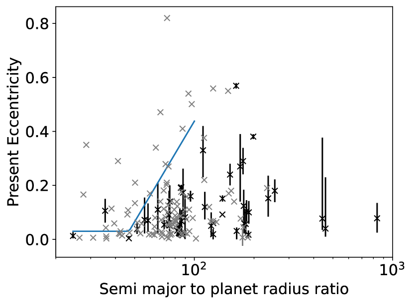
Figure 1: Eccentricity vs. semi-major axis to planet radius ratio for the hot Jupiter systems selected for analysis: orbital period less than 10 d, planet radius bigger than 0.6 Jupiter radii, stellar mass between 0.4 and 1.2 $M_{\odot}$.

The first step in our procedure is to define an eccentricity envelope: an upper limit to the eccentricity that a system with a given ratio of the semi-major axis to planet radius is allowed to have. There must be sufficient tidal dissipation to ensure that no matter the initial conditions with which tidal evolution begins, tidal circularization will drive the eccentricity below the envelope.

Figure 1 shows the scatter plot of present eccentricity vs. semi-major axis ($a$) divided by planetary radius ($R_{p}$) of different star-exoplanet systems. The gray crosses correspond to the systems for which only an upper limit on their present orbital eccentricity is available in the literature. The black crosses with error bars correspond to those systems for which both upper and lower uncertainties of the orbital eccentricity are provided. We see a clear signature of tidal circularization in this plot. When the semi-major axis is very large then tides are insignificant, and hence, the planetary orbits have a broad distribution of eccentricities, including very large values. As $\frac{a}{R_{p}}$ decreases, tides get stronger, and the distribution of observed eccentricities gradually narrows to smaller and smaller eccentricities. At even smaller semi-major axes, we see that there are almost no planets with clearly detected non-zero eccentricities. The evident exception is HAT-P-23 b, with $a/R_{p}=35.5$, for which the discovery paper (Bakos et al., 2011b) reports eccentricity of $0.11\pm 0.04$. However, conflicting data is found in Bonomo et al. (2017), who argue that observations are consistent with a circular orbit and only find an upper limit on the orbital eccentricity of 0.052. Due to the ambiguity in measured eccentricity, we exclude the HAT-P-23 system from this analysis.

Since the strength of tides is determined by the ratio of the planet size to the semi-major axis ($R_{p}/a$), that is the parameter we use for defining the eccentricity envelope. The solid line in Figure 1 shows the eccentricity envelope we assume for this analysis, given by:

$$e_{env}\big{(}\frac{a}{R_{p}}\big{)}=\begin{cases}0.03&\text{if }\frac{a}{R_{p}}<47.8\\ 0.03+1.27(\log\frac{a}{R{p}}-1.68)&\text{if }47.8<\frac{a}{R_{p}}<130\\ 0.6&\text{if }\frac{a}{R_{p}}>130\end{cases}$$ (19)

In the presence of tidal dissipation, whatever the initial eccentricity, initial period, and quality factor $Q$ may be, they must be such that the eccentricity ultimately becomes its present measured value. If the tidal dissipation is very large, then no matter how high the initial eccentricity is, the final calculated eccentricity at the present age will be below the present measured eccentricity. Thus, requiring that an initial eccentricity exists which evolves to the present-day eccentricity sets a maximum for the tidal dissipation, corresponding to a minimum value of the quality factor. On the other hand, no matter how high the initial eccentricity is the tidal dissipation should be high enough to shrink the eccentricity at the present time below the envelope eccentricity. That is the minimum tidal dissipation, corresponding to the maximum value of the quality factor.

The procedure for determining if a particular set of tidal dissipation parameters ($Q_{0}$, $P_{br}$, $\alpha$) is acceptable, while accounting for the unknown initial eccentricity, is described as follows. We find an initial orbital period such that the orbital evolution reproduces the present-day orbital period at the measured age of the system, starting with an over-estimated initial eccentricity ($e_{i}=0.8$) and the tidal dissipation parameters we wish to evaluate. Because starting with a lower initial eccentricity would result in a smaller predicted present-day eccentricity, if we find that the evolution ends with an eccentricity below the measured value for our system, we can reject the assumed dissipation parameters as too dissipative. If on the other hand, the final eccentricity is above the envelope, we reject the dissipation parameters as not dissipative enough. We accept all parameters which result in eccentricities between the measured present-day eccentricity and the envelope eccentricity for the $a/R_{p}$ of our target hot Jupiter system. We discuss how we deal with observational uncertainties in Section 3.4.

3.4 Bayesian Analysis

As mentioned in Section 3.2, for each individual hot Jupiter system, we want to find a joint distribution of $Q_{0}$, $\alpha$, and $P_{br}$ which is consistent with the observed eccentricity of that particular system and enforces the envelope eccentricity given the measured $a/R_{p}$. Given the large number of parameters that must be specified in order to calculate the evolution, we are restricted to generating samples from that joint distribution using a Markov Chain Monte Carlo (MCMC) algorithm. In particular, we will rely on the emcee python package (Foreman-Mackey et al., 2013), which implements an ensemble sampling algorithm that uses affine invariant transformation as a proposal function to simultaneously generate multiple correlated chains (known as walkers).

The full list of model parameters required to uniquely specify the orbital evolution is as follows:

1. $Q_{0}$: The minimum tidal quality factor of the planet (maximum dissipation) at any frequency (see Eq. 18).

2. $\alpha$: The power-law index of the frequency dependence of the planetary tidal quality factor (see Eq. 18).

3. $P_{br}$: The tidal period at which the planetary dissipation saturates (see Eq. 18).

4. $Q_{\star}$: The tidal quality factor of the star.

5. $M_{\star}$: mass of the parent star.

6. $M_{p}$: mass of the planet.

7. $\left[\frac{Fe}{H}\right]$: metallicity of the star.

8. $t$: Age of the system.

9. $R_{p}$: Radius of the planet.

10. $P_{spin,0}$: Initial spin period of the star.

Standard MCMC terminology splits the distribution we wish to sample from into priors for the model parameters and a likelihood function ($\mathcal{L}$). The priors we wish to impose are determined by the observational constraints available for the system. For most parameters, we assume independent Gaussian priors with mean and standard deviation taken directly from Table 1. However, for transiting planets, the constraints on the planet’s radius come from the transit depth. As a result, the uncertainties in the planetary and stellar radii are highly correlated. In an effort to account for this correlation, we use the square of the planet-to-star radius ratio $(R_{p}/R_{\star})^{2}$ as a parameter in lieu of the planet radius, whenever available. In those cases, the planet radius is calculated from the stellar radius predicted by POET’s stellar evolution modeling using the mass, age, and metallicity of the parent star of a particular sample.

For the tidal parameters and initial stellar spin, we use broad uniform priors:

$$\log_{10}Q_{0} \sim \mathcal{U}[3,12]$$

$$\log_{10}P_{br} \sim \mathcal{U}[\log_{10}(0.5\,d),\log_{10}(10\,d)]$$

$$\alpha \sim \mathcal{U}[-5,5]$$

$$\log_{10}Q_{\star} \sim \mathcal{U}[5,12]$$

$$P_{spin,0} \sim \mathcal{U}[5\,d,15\,d]$$

where $\mathcal{U}$ denotes a uniform distribution (in contrast to $U$ from before which denoted tidal potential).

In addition, several parameters are held fixed for all systems:

1. starting age for the tidal evolution: 20  Myrs

2. wind strength ($K_{w}$ in Eq. 16): 0.17  $M_{\odot}\,R_{\odot}^{2}\,\mathrm{day}^{2}\,\mathrm{rad}^{-2}\,\mathrm{Gyr}^{-1}$

3. wind saturation frequency ($\omega_{sat}$ in Eq. 16): 2.78  rad/day

4. stellar core-envelope coupling ($\tau_{c}$ in Eq. 15): 5 Myr

As we already discussed in section 3.3, we need to define our likelihood function ($\mathcal{L}$) to allow eccentricities anywhere between the present-day eccentricity of the system and the envelope that corresponds to the $a/R_{p}$ value for that system.

The first step is to specify the uncertainty distribution we will assume for the present-day eccentricity. We begin by noting that eccentricity ($e$) is not directly constrained by observations, but always in combination with the argument of periapsis ($\omega$). The complete details of the distribution of allowed eccentricity values given the observations of a particular system are a complicated function of the available radial velocity, photometry, and other observations. It is impractical to attempt to reconstruct these for every single system, especially given the disparate types, quantity, and quality of observations available in each case. Instead, we approximate the distribution by treating $e\cos\omega$ and $e\sin\omega$ as independent parameters, each following a Gaussian distribution. We further simplify the treatment by assuming that the standard deviations of the two distributions are the same. These assumptions imply that the eccentricity follows a Rice distribution. However, we must be careful with the prior we impose on $e$. By treating $e\cos\omega$ and $e\sin\omega$ as the variables, we are implicitly imposing a flat prior in that space. This will have the highly undesirable property that the probability of $e=0$ is always zero, no matter the available observational data, as a Rice distribution is always zero at the origin. Instead, we wish to impose a uniform prior on $e$. Switching from one prior to the other simply requires dividing by $e$ and renormalizing, resulting in the following distribution for the present-day eccentricity up to a normalization constant:

$$f(e)\propto\exp\left(-\frac{e^{2}+\mu^{2}}{2\sigma^{2}}\right)I_{0}\left(\frac{e\mu}{\sigma^{2}}\right)$$ (20)

where $\mu$ and $\sigma$ are parameters determining the distribution. They are related to the means ($\mu_{\cos}$ and $\mu_{\sin}$) and the standard deviation (assumed the same) of the Gaussian $e\cos\omega$ and $e\sin\omega$ distributions. Namely, $\mu=\sqrt{\mu_{\cos}^{2}+\mu_{\sin}^{2}}$, and $\sigma$ is the standard deviation (same for both components).

To determine the $\mu$ and $\sigma$ parameters, we consider two cases. When a two-sided confidence interval is available for the eccentricity (i.e $e=\bar{e}^{+\delta_{+}}_{-\delta_{-}}$ in Table 1), $\mu$ and $\sigma$ are found by requiring that the 15.9% and 84.1% quantiles of the Rice distribution (before correcting for the eccentricity prior) match the ends of the confidence interval:

$$0.159=\int_{0}^{\bar{e}-\delta_{-}}\frac{e}{\sigma^{2}}\exp\left(-\frac{e^{2}+\mu^{2}}{2\sigma^{2}}\right)I_{0}\left(\frac{e\mu}{\sigma^{2}}\right)de$$ (21)

$$0.841=\int_{0}^{\bar{e}+\delta_{+}}\frac{e}{\sigma^{2}}\exp\left(-\frac{e^{2}+\mu^{2}}{2\sigma^{2}}\right)I_{0}\left(\frac{e\mu}{\sigma^{2}}\right)de$$ (22)

When observations cannot exclude the possibility of a circular orbit, only an upper limit is available for the eccentricity, we set $\mu=0$ and find $\sigma$ by requiring that the cumulative Rice distribution (before correcting for the eccentricity prior) matches the confidence level of the given limit.

Having defined a distribution for the present-day eccentricity, the next step is to define the likelihood of our MCMC analysis. Given values for all model parameters, let $\epsilon(e_{i})$ be the function that gives the final eccentricity the orbital evolution would result in, if started with an initial eccentricity $e_{i}$ and orbital period such that the present-day orbital period is reproduced. Furthermore, let $e_{env}$ be the envelope eccentricity for the given system, $e_{i}^{max}$ be the maximum initial eccentricity we consider (in our case $e_{i}^{max}=0.8$), and $\pi(e_{i})$ be a prior we wish to impose on the initial eccentricity (the distribution of orbital eccentricities with which planets begin their tidal evolution). Then up to a normalization constant, the likelihood that the selected model parameters are the true values is:

$$\mathcal{L}\propto H\left[\epsilon(e_{i}^{max})-e_{env}\right]\int_{0}^{e_{i}^{max}}f\left[\epsilon(e_{i})\right]\pi(e_{i})de_{i}$$ (23)

where the Heaviside step function $H\left[\epsilon(e_{i}^{max})-e_{env}\right]$ imposes the requirement that no initial conditions should result in present day eccentricity above the envelope, and the integral gives the likelihood of the system evolving to the observed present-day eccentricity. We do not know the distribution of initial eccentricities exoplanets start with ($\pi(e_{i})$) and finding $\epsilon(e_{i})$ is impractical, so we only evaluate $\epsilon\left(e_{i}^{max}\right)$. However, the integral in Eq. 23 is a weighted average of $f(e)$, so we approximate the likelihood as:

$$\mathcal{L}\propto\begin{cases}\frac{1}{e^{max}}\int_{0}^{e^{max}}f(e)de&\text{if }e^{max}\leq e_{env}\\ 0&\text{otherwise}\end{cases}$$ (24)

where $e^{max}\equiv\epsilon(e_{i}^{max})$ is the present day eccentricity our evolution found after starting with $e_{i}^{max}=0.8$.

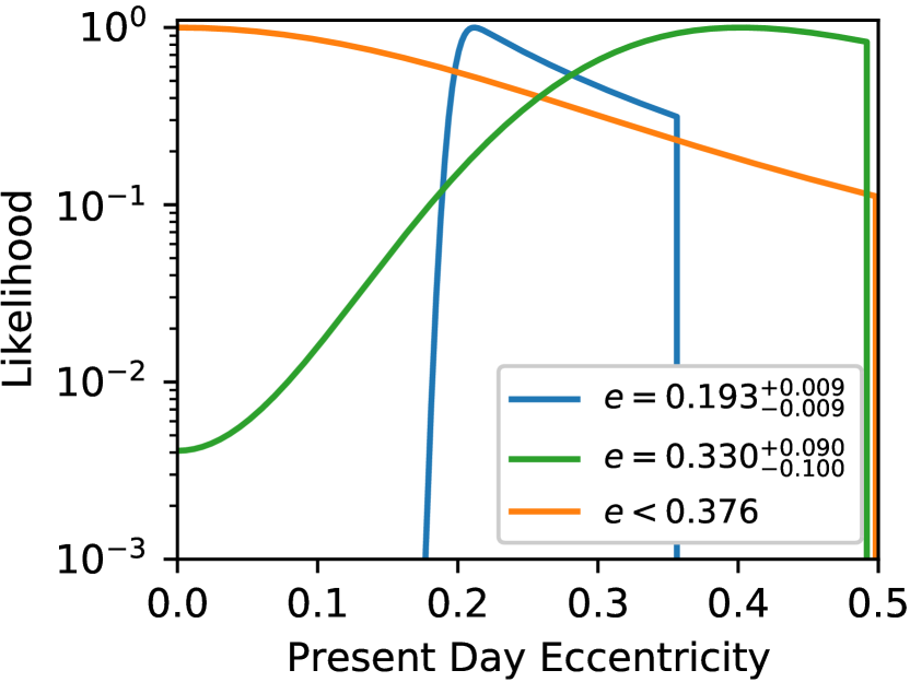
Figure 2: Example likelihood functions for a clearly eccentric system, WASP-89 b (blue); a system for which a circular orbit is disfavored but not fully ruled out, CoRoT-16 b (green); and a system with only an upper limit on the eccentricity, HATS-8 b (orange).

Fig. 2 shows examples of the likelihood functions for three different exoplanet systems: WASP-89 b for which a circular orbit is ruled out to very high significance, CoRoT-16 b for which the available observations clearly prefer a non-circular orbit but cannot entirely rule out $e=0$, and HATS-8 b for which only an upper limit is available for the eccentricity.

Fig. 3 demonstrates the full MCMC analysis for one hot Jupiter system: WASP-89 b. The left panel shows the eccentricity envelope and the observed eccentricity for the system, the middle panel shows the resulting likelihood function and the right panel shows the MCMC analysis. The green line shows the final eccentricity as a function of $Q_{pl}^{\prime}$ assuming a constant $Q_{pl}^{\prime}$ model (i.e. $\alpha=0$ in Eq. 18), $Q_{\star}^{\prime}=10^{6}$ and fixing all system properties to their nominal values. The points correspond to the MCMC samples of frequency-dependent $Q_{pl}^{\prime}$ (per Eq. 18). For each MCMC sample, we evaluated Eq. 18 at a tidal period of 2  days, which is the tidal period this particular system is most sensitive to, i.e. where that particular system gives the tightest constraints on $Q_{pl}^{\prime}$.

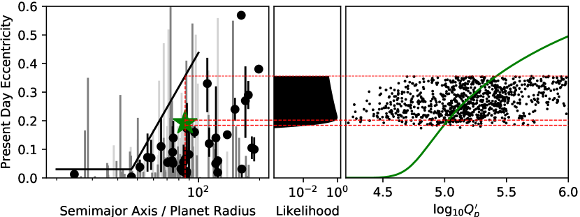
Figure 3: Demonstration of the tidal circularization method for constraining $Q_{pl}^{\prime}$. Left: The eccentricity envelope (black line) using the observed present-day eccentricities of HJs. Middle: The likelihood function, requiring that dissipation is large enough to circularize the system to below the envelope no matter how large the initial eccentricity is while allowing the observed present-day eccentricity to be reproduced. Right: MCMC samples for $Q_{pl}^{\prime}(P_{tide}=2\,d)$ (points), and the relation between predicted present-day eccentricity and $Q_{pl}^{\prime}$ (green curve) for nominal system parameters, and $Q_{\star}^{\prime}=10^{6}$. $Q_{pl}^{\prime}$ was assumed constant only for finding the green curve, otherwise, Eq. 18 was used.

3.5 Constraining Frequency Dependent $Q_{pl}^{\prime}$ and Convergence Test

A particularly useful approach for building constraints for the value of $Q_{pl}^{\prime}$ at each tidal period begins by evaluating Eq. 18 for each MCMC sample of a given system on a grid of tidal periods, obtaining samples of $Q_{pl}^{\prime}(P_{tide},R_{pl})$ at each grid point. After that, again at each of the grid points, we create a kernel density estimate of the probability distribution of $Q_{pl}^{\prime}(P_{tide})$ for each system. Finally, the probability distributions of all systems at a given grid point are multiplied together and re-normalized to get a combined constraint. Since each individual system probes a relatively narrow range of tidal periods, the combined constraint produced in this fashion is no longer restricted to a purely power-law dependence of $Q_{pl}^{\prime}$, but rather Eq. 18 simply ensures continuity and our prior on $\alpha$ imposes a limit on the maximum slope of the dependence of $\log_{10}Q_{pl}^{\prime}$ on $\log_{10}P_{tide}$. When combining constraints, we apply one additional consideration. Because each individual binary is sensitive only to the dissipation in a relatively narrow range of periods, it produces tight constraints on $Q_{pl}^{\prime}(P_{tide})$ only in that range. Moving away from that period, the spread in allowed values of $Q_{pl}^{\prime}(P_{tide})$ is limited by the prior we impose on $\alpha$. When building the combined constraints, for each binary we identify the range of periods where the constraints are tightest and only include that binary in the combined constraint for the $P_{tide}$ grid points within that range.

MCMC sampling using the emcee (Foreman-Mackey et al., 2013) package involves advancing multiple (in our case 64) chains that are not statistically independent. Since we don’t know a priori how the likelihood function looks, we initialize the chains with samples that are over-dispersed compared to the equilibrium posterior distribution. The chains gradually migrate to higher likelihood regions until the equilibrium distribution is found. As a result, early samples tend to overestimate the uncertainties, and possibly introduce bias in estimated values. The usual practice is to discard these so-called ‘burn-in’ initial samples. We thus need a method to estimate this burn-in period for our samples. Subsequently, we need an estimate of how many additional iterations need to be accumulated to get reliable estimates of the desired quantities and their uncertainty distributions.

In this work, we are aiming to measure the quantiles of the distribution of $Q_{pl}^{\prime}$ at a grid of tidal periods. The method of determining the number of burn-in steps required to reach close to the equilibrium distribution, and the number of steps required after the burn-in to measure the value of the cumulative distribution function at each quantile with a desired precision is discussed in Patel & Penev (2022) and Penev & Schussler (2022). The method developed in these papers is an extension of the method discussed in Raftery & Lewis (1991), adapting it for use with multiple interdependent chains. We have applied the same method discussed in these papers to perform a convergence analysis of the MCMC process in this project.

Essentially, for each quantile ($q$) the algorithm finds a simultaneous burn-in period ($N_{b}$) and quantile values that meet the following two conditions:

1. The distribution of the fraction of the 64 $N_{b}+1$ samples smaller than $q$ is within $10^{-3}$ of the distribution after infinitely many steps.

2. The fraction of all samples after $N_{b}$ below $q$ is equal to the target quantile.

That same algorithm also provides an estimate of the standard deviation of the fraction of samples below $q$ over different realizations of a chain of a given length. This is a measure of how precisely a given quantile is estimated.

4 Results

4.1 Individual Constraints

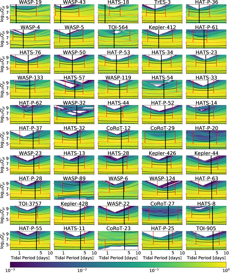
Figure 4: Constraints on $\log_{10}Q^{\prime}_{pl}$ for tidal periods in the range $0.5\,d<P_{tide}<10\,d$ for each individual star-exoplanet system. The color indicates the probability density of $\log_{10}Q^{\prime}_{pl}$ at each tidal period. The thick black vertical line shows the system’s orbital period. The left-to-right red curve shows the median of the $\log_{10}Q^{\prime}_{pl}(P_{tide})$ distribution at each tidal period. Similarly, the four black curves from bottom to top represent the 2.3, 15.9, 84.1, and 97.7 percentiles, respectively, of the distribution of $\log_{10}Q^{\prime}_{pl}$ at each tidal period. In the region between the two vertical red lines, we consider the constraints to be driven by the available measurements for that system, instead of by the prior we place on the period dependence power-law index $\alpha$ (see text for details).

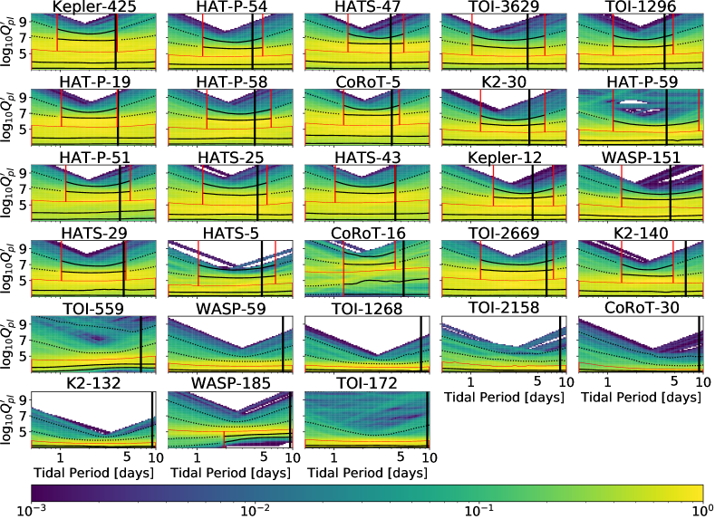
Figure 5: Continuation of Figure 4.

Figures 4 and 5 show the constraints on $\log_{10}Q^{\prime}_{pl}$ for different tidal periods, $P_{tide}\in[0.5,10]$ days for each individual star-exoplanet system. For every sample of the MCMC, the values of the parameters ($\alpha$, $P_{br}$ and $Q_{0}$) are used to calculate $Q_{pl}^{\prime}(P_{tide})$ using Eq. 18 at a grid of tidal periods. Thus, for each system at every value of $P_{tide}$, we get samples of $\log_{10}Q^{\prime}_{pl}$ required by the observed and envelope eccentricities of the system. Using Kernel Density Estimation (KDE) with an Epanechnikov kernel function with a width of 0.2 dex, we construct an estimate of the probability density function (PDF) of $\log_{10}Q^{\prime}_{pl}(P_{tide})$ at each tidal period. The color along each vertical slice of a panel in Fig. 4 and Fig. 5 shows that PDF at the tidal period of the slice. The thick black vertical line shows the orbital period of the system. The thin red curve going from left to right shows the median of that PDF at each tidal period, and the black curves from the bottom to top show the 2.3, 15.9, 84.1, and 97.7 percentiles, respectively. Only samples after the automatically determined burn-in period were used to generate Fig. 4 and 5.

A common feature seen in many of the individual constraints is that for a given system, $Q_{pl}^{\prime}$ is only constrained for a narrow range of tidal periods, and moving away from that, the distribution of allowed $Q_{pl}^{\prime}$ values gets much broader. This is caused by the fact that for an individual system, tidal circularization is dominated by a narrow range of tidal periods. As we plan to use the individual constraints to build a combined constraint, for each system we need to define the range of tidal periods that the system is sensitive to (which we dub the reliable period range) and only include its constraints at those tidal periods. In fact, for each system, we define two reliable period ranges – one for the upper half and one for the lower half of the distribution. These ranges are defined using a very simple criterion. Namely, for the upper/lower half of the distribution, the range is defined by requiring that the 97.7%/2.3% percentile is within 0.7 dex of its minimum/maximum value. The reliable period ranges are delineated by the vertical red lines in each plot (one set for the distribution above the median and another set for the distribution below).

Figures 6 and 7 show the estimated burn-in period. The solid portions of the curves correspond to the reliable period range for each quantile where the results are dominated by observational data. The dotted portions of the curves are outside the reliable period range. The black region depicts the total number of emcee steps accumulated for that system. As these figures demonstrate, for all systems we have generated sufficient samples to exceed the burn-in period for each quantile of $Q_{pl}^{\prime}$ for each tidal period within the reliable period range.

Figures 8 and 9 show the standard deviation of the value of the cumulative density function at the estimated value of the four percentiles ($\sigma_{CDF}$) for different values of $P_{tide}$ for the steps of MCMC, generated in the post-burn-in epoch. We see that for all systems, $\sigma_{CDF}<<\min(CDF,1-CDF)$ for each quantile. In other words, the fraction of samples outside a given confidence interval is estimated with high precision (small uncertainty). For example, for WASP-19, the fraction of samples below the 15.9% percentile is within 1% or better of 15.9% for all tidal periods.

Figures 4 and 5 show that for most of the star-exoplanet systems, we get a sharp upper limit for $\log_{10}Q^{\prime}_{pl}$ for a range of values of $P_{tide}$. If the value of $\log_{10}Q^{\prime}_{pl}$ is greater than this upper limit then the tidal dissipation is not strong enough to shrink the orbital eccentricity below the envelope eccentricity for the system in the scatter plot of eccentricity vs. $\log(\frac{a}{R_{p}})$. On the other hand, except for WASP-89 b, CoRoT-23 b, and WASP-185 b, the lower limits are less sharp, though for many systems the likelihood drops off substantially for low $Q_{pl}^{\prime}$ values (note that the color scale in the plots is logarithmic).

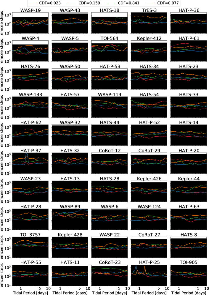
Figure 6: Estimated emcee steps required to reach close to the equilibrium value of the percentiles of $\log_{10}Q^{\prime}_{pl}$ as a function of $P_{tide}$. Within the solid portion of the curves, constraints are influenced by the observation and hence are reliable. The dotted portion of the curves is influenced by our prior assumptions. The black area represents the number of steps completed.

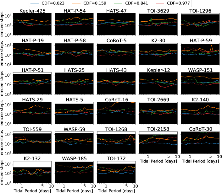
Figure 7: Continuation of Figure 6.

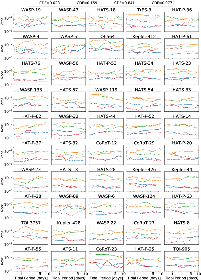
Figure 8: The standard deviation of the cumulative density function of $\log_{10}Q^{\prime}_{pl}$ up to the indicated percentile as a function of $P_{tide}$. Within the solid portion of the curves, constraints are influenced by the observations and hence are reliable. The dotted portion of the curves is influenced by our prior assumptions.

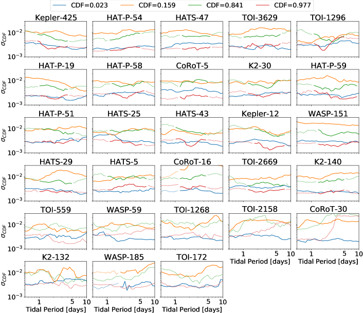
Figure 9: Continuation of Figure 8.

For CoRoT-23 b, our analysis shows lower limits of $\log_{10}Q^{\prime}_{pl}$ for a range of values of $P_{tide}$. Had the $\log_{10}Q^{\prime}_{pl}$ been less than the lower limit for any value of $P_{tide}$ within that range, the tidal dissipation would become so strong that the orbital eccentricity of the system at present age would have been smaller than the actual orbital eccentricity the system has now. We require that the tidal dissipation not be that strong, as the system started the evolution with a very high orbital eccentricity of 0.8. However, as mentioned in Section 2, the significantly non-zero value of the eccentricity we used for the analysis (reported by Rouan et al. (2012)) has been disputed (Bonomo et al., 2017). As a result, we show the individual constraints for CoRoT-23 b but do not include them when constructing the combined constraints on $\log_{10}Q^{\prime}_{pl}$.

4.2 Combined Constraints

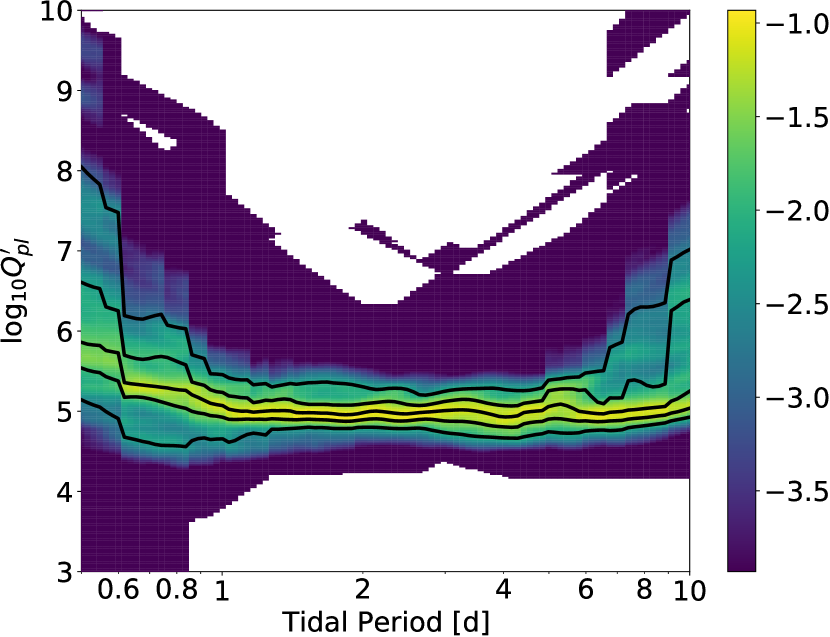
Figure 10: Combined constraints for $\log_{10}Q^{\prime}_{pl}$ assuming a common frequency dependent dissipation applies to all planets from Table 1 except CoRoT-23 b. The color shows $\log_{10}$ of the combined probability. The five black curves from the bottom to top show the 2.3%, 15.9%, 50.0%, 84.1%, and 97.7% percentiles of the $\log_{10}Q^{\prime}_{pl}$ distribution at each tidal period. For every $P_{tide}$, the combined posterior probability density distribution of $\log_{10}Q^{\prime}_{pl}$ is the product of the posterior probability density distribution of $\log_{10}Q^{\prime}_{pl}$ for individual systems for which that tidal period falls within the reliable period range.

Next, we combine the constraints on $\log_{10}Q^{\prime}_{pl}$ for individual exoplanet systems to build constraints for the tidal quality factor under the assumption that the planets in our sample are similar enough to share the same tidal dissipation. In order to do so, for each tidal period ($P_{tide}$), we multiply together the individual probability density functions for $\log_{10}Q^{\prime}_{pl}(P_{tide})$. The product only includes posterior probability density functions of $\log_{10}Q^{\prime}_{pl}$ for systems for which a given tidal period falls within the reliable period range. If a tidal period falls in the range of the tidal periods of a particular system for which only upper/lower percentiles above/below the median are reliable then we replace the unreliable lower/upper portion of the probability density of $\log_{10}Q^{\prime}_{pl}$ with the probability density of its median at that tidal period and re-normalize the distribution before including it. The resulting product of PDFs is then normalized to unit integral.

When building the combined constraints we exclude three systems: CoRoT-23 b, K2-132 b, and TOI-2669 b. CoRoT-23 b was excluded because its eccentricity measurement is suspect, as explained before. K2-132 b and TOI-2669 b were excluded because their host stars have evolved to their red giant phase. For such ages, the POET handling of stellar evolution is potentially suspect as it involves interpolating among fast-evolving post-main-sequence portions of the stellar evolution tracks.

In addition, per Eq. 19 we imposed an envelope eccentricity of 0.6 for systems with $a/R_{p}>130$ which is not physically justified. Conservative assumption would suggest that for those systems there is no observable tidal circularization. To account for that, we exclude the upper limit on $\log_{10}Q^{\prime}_{pl}$ for these systems: CoRoT-30 b, WASP-59 b, WASP-185 b, TOI-559 b, K2-132 b, TOI-2158 b, TOI-172 b, TOI-1268 b. In practice, this means that from these systems, only WASP-18 b contributes to the combined constraint, giving a lower limit to $Q_{pl}^{\prime}$ at the longest tidal periods studied.

Figure 10 shows the resulting combined constraint for $\log_{10}Q^{\prime}_{pl}$ for the period range $0.5\,d<P_{tide}<10\,d$. The color shows $\log_{10}$ of the combined probability, and the black curves, from bottom to top, represent 2.3%, 15.9%, 50%, 84.1%, and 97.7% percentiles of the $\log_{10}Q^{\prime}_{pl}$ distribution at each tidal period, respectively.

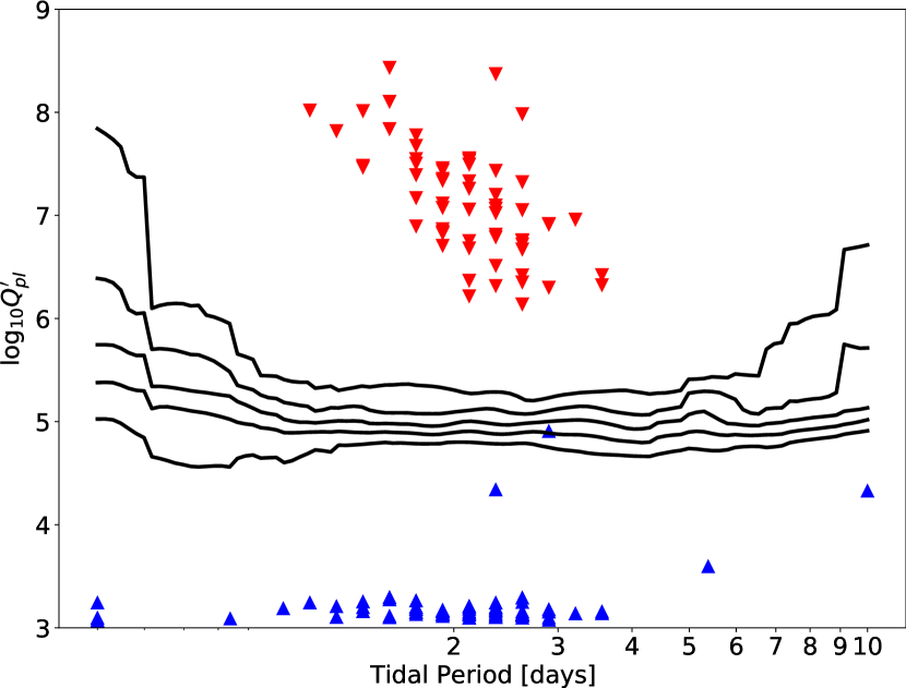
Figure 11: Black curves: 2.3%, 15.9%, 50.0%, 84.1%, and 97.7% percentiles of the $\log_{10}Q^{\prime}_{pl}$, as in Fig. 10. Red (blue) triangles pointing downward (upward) show the 97.7% (2.3%) percentile of the constraint for an individual system at the tidal period where for that particular system the quantile is the lowest (highest).

The combined constraint is only meaningful if the individual constraints are actually consistent with each other. Fig. 11 compares the combined constraints with the constraints for individual systems. The five black curves are as described in the previous paragraph for Fig. 10. For each system, a red and a blue triangle are shown, indicating the minimum of the 97.7% and the maximum of the 2.3% percentiles for that system’s constraints.

To see why the combined constraint is significantly tighter than even the tightest individual constraints, consider for example what would be required for $Q_{pl}$ to be near the lower limit for individual systems. Ignoring for a moment the uncertainties in anything other than present-day eccentricity, the lower limit on $Q_{pl}$ comes from starting the evolution with an initial eccentricity of $e_{i}=0.8$ and landing near the lower limit of the observationally determined distribution of the present-day eccentricity. Thus, this would imply that all literature eccentricities are systematically 2-$\sigma$ below the implied maximum likelihood value. More realistically, the true values of the present-day eccentricity, stellar mass, and stellar age must be simultaneously below the maximum likelihood values reported by about 1-$\sigma$, while the planet’s mass and radius must be above by about 1-$\sigma$ systematically for all exoplanet systems. Similarly, the 97th percentile of $Q_{pl}$ for each individual system comes from assuming systematically larger age and planet radius, combined with systematically smaller stellar mass.

As Fig. 11 shows, the combined constraints are consistent with all individual constraints, even for the systems that were excluded from the combined constraint due to suspicion that the stellar interpolation may not be reliable or for the one with disputed eccentricity measurement. Table 2 shows the comparison in tabular form.

We see that, for $P_{tide}$ between 0.8 and 7 days, the combined constraints on $\log_{10}Q^{\prime}_{pl}$ restrict its value to a very narrow range, and apart from the two exceptions are consistent with all individual constraints. We also see that the black curves are approximately parallel to the x-axis, implying that $\log_{10}Q^{\prime}_{pl}$ is approximately independent of the tidal period, and over that period range, typical hot Jupiter planets have $\log_{10}Q^{\prime}_{pl}=5.0\pm 0.5$.

Table 2: Comparison of combined and individual percentiles of $\log_{10}Q^{\prime}_{pl}$ for the $P_{tide}$ values at which each system provides the tightest constraints.

		Individual Quantiles of $\log_{10}Q^{\prime}_{p}$					Combined Quantiles of $\log_{10}Q^{\prime}_{p}$
System	$\mathbf{P_{tide}}$	2.3%	15.9%	50.0%	84.1%	97.7%	2.3%	15.9%	50.0%	84.1%	97.7%
WASP-19 b	1.56	3.27	4.03	5.63	7.14	8.10	4.79	4.90	4.98	5.09	5.36
WASP-43 b	1.14	3.24	3.97	5.55	7.14	8.02	4.70	4.90	4.99	5.14	5.36
HATS-18 b	1.56	3.11	3.87	5.58	7.43	8.43	4.79	4.90	4.98	5.09	5.36
TrES-3 b	1.40	3.20	3.84	5.36	6.72	7.48	4.78	4.89	5.00	5.14	5.34
HAT-P-36 b	1.27	3.21	4.01	5.22	7.03	7.82	4.75	4.90	5.01	5.13	5.31
WASP-4 b	1.56	3.30	4.00	5.74	7.14	7.84	4.79	4.90	4.98	5.09	5.36
WASP-5 b	2.12	3.20	3.98	5.23	6.52	7.50	4.80	4.91	5.00	5.11	5.27
TOI-564 b	1.03	3.19	4.00	5.54	7.22	10.78	4.61	4.90	5.03	5.19	5.41
Kepler-412 b	1.73	3.18	3.86	5.31	6.67	7.51	4.79	4.89	4.97	5.08	5.35
HAT-P-61 b	1.40	3.16	3.87	5.14	6.32	7.47	4.78	4.89	5.00	5.14	5.34
HATS-76 b	1.73	3.20	3.97	5.14	6.25	6.90	4.79	4.89	4.97	5.08	5.35
WASP-50 b	1.73	3.15	3.80	5.10	6.37	7.17	4.79	4.89	4.97	5.08	5.35
HAT-P-53 b	1.92	3.16	4.04	5.55	6.73	7.44	4.79	4.88	4.96	5.08	5.33
HATS-34 b	1.73	3.20	4.02	5.33	6.80	7.55	4.79	4.89	4.97	5.08	5.35
HATS-23 b	2.12	3.18	3.95	5.46	6.86	7.53	4.80	4.91	5.00	5.11	5.27
WASP-133 b	1.73	3.18	3.92	5.32	6.69	7.78	4.79	4.89	4.97	5.08	5.35
HATS-57 b	2.12	3.14	3.72	4.71	5.62	6.22	4.80	4.91	5.00	5.11	5.27
WASP-119 b	2.12	3.14	3.78	5.06	6.47	7.33	4.80	4.91	5.00	5.11	5.27
HATS-54 b	0.50	3.24	3.95	5.33	6.98	11.77	5.03	5.38	5.75	6.39	7.84
HATS-33 b	1.92	3.14	3.78	5.02	6.09	6.83	4.79	4.88	4.96	5.08	5.33
HAT-P-62 b	1.73	3.16	3.85	5.21	6.40	7.68	4.79	4.89	4.97	5.08	5.35
WASP-32 b	0.84	3.09	3.50	4.51	5.61	9.96	4.57	5.02	5.24	5.48	5.93
HATS-44 b	1.73	3.26	4.05	5.41	6.73	7.39	4.79	4.89	4.97	5.08	5.35
HAT-P-52 b	2.12	3.10	3.75	4.84	6.02	6.68	4.80	4.91	5.00	5.11	5.27
HATS-14 b	1.92	3.16	3.73	4.84	6.03	6.84	4.79	4.88	4.96	5.08	5.33
HAT-P-37 b	1.92	3.11	3.67	4.85	6.09	6.87	4.79	4.88	4.96	5.08	5.33
HATS-32 b	1.92	3.14	3.79	5.16	6.38	7.08	4.79	4.88	4.96	5.08	5.33
CoRoT-12 b	2.12	3.18	4.04	5.55	6.72	7.56	4.80	4.91	5.00	5.11	5.27
CoRoT-29 b	2.61	3.16	3.86	5.13	6.31	9.36	4.79	4.89	4.98	5.08	5.22
HAT-P-20 b	1.73	3.13	3.70	4.75	5.85	9.78	4.79	4.89	4.97	5.08	5.35
WASP-23 b	1.92	3.16	3.78	4.93	5.99	6.71	4.79	4.88	4.96	5.08	5.33
HATS-13 b	2.61	3.13	3.73	4.99	6.18	7.05	4.79	4.89	4.98	5.08	5.22
HATS-28 b	2.35	3.17	3.80	4.98	6.29	7.20	4.78	4.88	4.98	5.12	5.29
Kepler-426 b	1.92	3.13	3.72	5.29	6.54	7.36	4.79	4.88	4.96	5.08	5.33
Kepler-44 b	2.35	3.10	3.61	4.71	5.73	6.51	4.78	4.88	4.98	5.12	5.29
HAT-P-28 b	2.35	3.12	3.68	4.96	6.27	7.03	4.78	4.88	4.98	5.12	5.29
WASP-89 b	2.35	4.34	4.82	5.34	6.15	8.37	4.78	4.88	4.98	5.12	5.29
WASP-6 b	2.12	3.21	4.08	5.83	6.86	7.55	4.80	4.91	5.00	5.11	5.27
WASP-124 b	2.89	3.10	3.67	4.65	5.68	6.30	4.75	4.89	5.00	5.11	5.23
HAT-P-63 b	2.61	3.12	3.67	4.91	6.12	6.75	4.79	4.89	4.98	5.08	5.22
TOI-3757 b	1.92	3.17	4.07	5.38	6.64	7.34	4.79	4.88	4.96	5.08	5.33
Kepler-428 b	2.12	3.12	3.65	4.74	5.93	6.75	4.80	4.91	5.00	5.11	5.27
WASP-22 b	2.12	3.10	3.54	4.51	5.51	6.37	4.80	4.91	5.00	5.11	5.27
CoRoT-27 b	1.56	3.10	3.53	4.39	6.26	10.72	4.79	4.90	4.98	5.09	5.36
HATS-8 b	1.40	3.25	4.10	5.47	6.78	8.01	4.78	4.89	5.00	5.14	5.34
HAT-P-55 b	2.12	3.16	3.85	5.04	6.18	7.06	4.80	4.91	5.00	5.11	5.27
HATS-11 b	2.35	3.19	4.03	5.28	6.36	7.07	4.78	4.88	4.98	5.12	5.29
CoRoT-23 b	2.89	4.91	5.45	6.58	9.73	11.66	4.75	4.89	5.00	5.11	5.23
HAT-P-25 b	2.35	3.20	3.95	5.02	6.02	6.79	4.78	4.88	4.98	5.12	5.29
TOI-905 b	2.61	3.13	3.65	4.66	5.88	6.72	4.79	4.89	4.98	5.08	5.22
Kepler-425 b	1.92	3.16	3.85	5.21	6.65	7.46	4.79	4.88	4.96	5.08	5.33
HAT-P-54 b	2.61	3.13	3.63	4.66	5.63	6.42	4.79	4.89	4.98	5.08	5.22
HATS-47 b	2.89	3.15	3.89	5.12	6.23	6.92	4.75	4.89	5.00	5.11	5.23
TOI-3629 b	2.61	3.12	3.73	4.68	5.70	6.67	4.79	4.89	4.98	5.08	5.22
TOI-1296 b	2.61	3.14	3.71	4.84	5.83	6.76	4.79	4.89	4.98	5.08	5.22
HAT-P-19 b	1.92	3.16	3.93	5.29	6.41	7.12	4.79	4.88	4.96	5.08	5.33
HAT-P-58 b	2.89	3.18	3.91	5.03	6.13	6.91	4.75	4.89	5.00	5.11	5.23
CoRoT-5 b	2.35	3.24	4.16	5.46	6.77	7.44	4.78	4.88	4.98	5.12	5.29
K2-30 b	2.61	3.12	3.63	4.64	5.48	6.14	4.79	4.89	4.98	5.08	5.22
HAT-P-59 b	1.27	3.10	3.57	4.72	5.96	10.67	4.75	4.90	5.01	5.13	5.31
HAT-P-51 b	2.61	3.25	4.06	5.46	6.50	7.33	4.79	4.89	4.98	5.08	5.22
HATS-25 b	2.35	3.13	3.85	4.96	6.24	7.10	4.78	4.88	4.98	5.12	5.29
HATS-43 b	2.12	3.16	3.87	5.28	6.45	7.26	4.80	4.91	5.00	5.11	5.27
Kepler-12 b	3.56	3.16	3.76	4.83	5.85	6.42	4.68	4.85	4.99	5.12	5.29
WASP-151 b	3.56	3.14	3.58	4.70	5.66	6.33	4.68	4.85	4.99	5.12	5.29
HATS-29 b	2.35	3.15	3.88	4.96	5.98	6.82	4.78	4.88	4.98	5.12	5.29
HATS-5 b	2.35	3.10	3.53	4.37	5.34	6.32	4.78	4.88	4.98	5.12	5.29
CoRoT-16 b	2.61	3.29	5.02	6.23	7.01	7.98	4.79	4.89	4.98	5.08	5.22
TOI-2669 b	3.21	3.14	3.86	5.00	6.16	6.96	4.71	4.87	5.02	5.15	5.28
K2-140 b	2.61	3.10	3.66	4.72	5.59	6.35	4.79	4.89	4.98	5.08	5.22
TOI-559 b	5.38	3.60	4.02	4.76	nan	nan	4.72	4.89	5.08	5.29	5.43
WASP-59 b	0.50	3.05	3.33	4.14	nan	nan	5.03	5.38	5.75	6.39	7.84
TOI-1268 b	0.50	3.07	3.34	3.89	nan	nan	5.03	5.38	5.75	6.39	7.84
TOI-2158 b	0.50	3.10	3.49	4.29	nan	nan	5.03	5.38	5.75	6.39	7.84
CoRoT-30 b	0.50	3.08	3.38	4.24	nan	nan	5.03	5.38	5.75	6.39	7.84
K2-132 b	0.50	3.04	3.27	3.90	nan	nan	5.03	5.38	5.75	6.39	7.84
WASP-185 b	10.00	4.33	4.82	5.33	nan	nan	4.91	5.02	5.13	5.71	6.71
TOI-172 b	2.89	3.08	3.32	3.80	nan	nan	4.75	4.89	5.00	5.11	5.23

The above result ignores the thermal evolution of the planet. Tidal heating of a planet can affect its size and hence change the rate of orbital evolution (Alvarado-Montes & García-Carmona, 2019; Rozner et al., 2022). If the planets are initially large, the cooling process tries to shrink their radius. Planets start out large and cool and shrink over time. Tidal heating can slow down this shrinking or even reverse it. As a result, planets would have had larger radii in the past than they do today, potentially lasting long enough to imply noticeably faster circularization for a given value of $Q_{pl}^{\prime}$. The extent to which this would affect the inferred value of $Q_{pl}^{\prime}$ depends on how long these larger radii persisted and on the physical mechanisms driving tidal dissipation. For example, if visco-elastic dissipation in the solid core of planets dominates, tidal heating will have relatively little effect on the circularization rate, i.e. the effective $Q_{pl}^{\prime}$ will scale with the planet’s radius in such a way as to approximately cancel the radius dependence from the rate of tidal circularization (assuming the core mass and radius do not change as the planet cools). If inertial mode dissipation dominates, it also depends on the ratio of the core’s radius to the whole radius of the planet (Guenel et al., 2014b), though not sufficiently as to completely cancel the radius dependence.

We have assumed that the observational uncertainties of the physical properties of the systems (planet and star mass, age, metallicity, planet radius, orbital eccentricity) are independent Gaussian distributions. By ignoring the correlations between planetary and stellar properties we are inflating the uncertainty in the measurement of the tidal quality factor. For example, tidal evolution is only sensitive to the planet-to-star mass ratio, which is usually constrained much more tightly by radial velocity observations than each mass separately. Sampling each mass independently results in a much broader distribution of mass ratios. Similarly, for many systems, the planet-to-star radius ratio is not included in the Exoplanet Archive, so we impose a Gaussian prior on the planet radius directly. Once again this results in a broader distribution of planet-to-star size ratios, translating to larger inferred uncertainty in $\log_{10}Q_{pl}^{\prime}$. For those systems for which the square radius ratio is provided, we impose a prior on it and infer the planet radius from the stellar radius the built-in POET stellar evolution predicts for the sampled stellar mass, age, and metallicity.

5 Comparison to Prior Tidal Dissipation Constraints

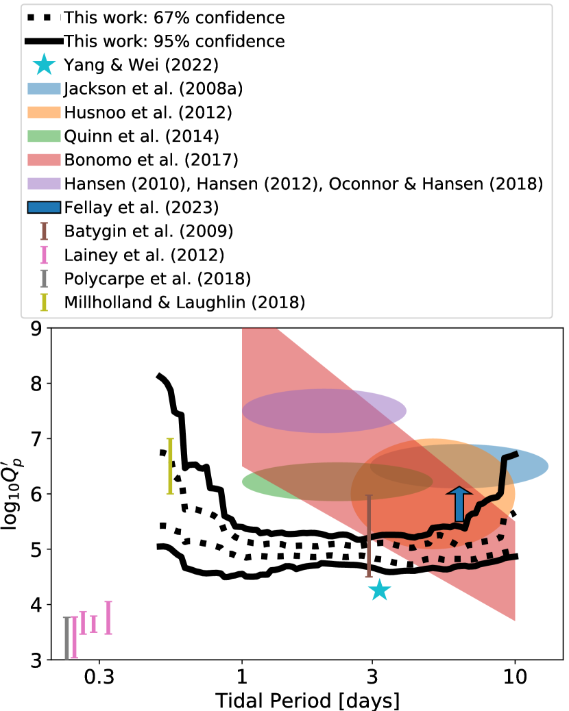
Figure 12: The combined constraint on $\log_{10}Q^{\prime}_{pl}$ as a function of the tidal period from our analysis of 77 HJ systems (see text) demonstrating the expected precision and period range over which tidal dissipation will be constrained by this project. The solid lines show the 95% confidence interval (2.3% and 97.7% percentiles of the combined posterior distribution), and the dotted lines show the 68% confidence interval (15.9% and 84.1% percentiles).

Figure 12 summarizes the comparison between our constraints and the constraints on $Q_{pl}^{\prime}$ found in the literature. Below we discuss in more detail each of the constraints shown in the figure as well as two additional analyses which only provide a lower limit to $Q_{pl}^{\prime}$.

Jackson et al. (2008) tuned the values of $Q_{pl}^{\prime}$ and $Q_{\star}^{\prime}$ (assumed constant) by requiring that the initial eccentricity distribution for orbital semi-major axes below 0.2 AU matches that of larger orbits. They found the best fit based on a Kolmogorov-Smirnov test for $Q_{pl}^{\prime}=10^{6.5}$ and $Q_{\star}^{\prime}=10^{5.5}$. Their estimated value of $Q_{pl}$ is an order of magnitude larger than our finding. The majority of the planets used by Jackson et al. (2008) were detected through radial velocity observations. As a result, for the majority of their planets, only a lower limit was available for the planetary mass due to the unknown orbital inclination, and the planetary radius was not directly constrained by observations. For such planets, Jackson et al. (2008) assumed the planet mass is equal to the minimum mass, and for gas giant planets assumed a radius of 1.2 Jupiter radii. Perhaps less importantly, the tidal evolution model used by Jackson et al. (2008) ignored stellar evolution and only included first-order eccentricity terms. Since these authors are investigating the same tidal signature as us, the difference in inferred $Q_{pl}^{\prime}$ values must be driven by some combination of the superior parameters provided by transiting planets, the larger sample size at our disposal, the somewhat different statistical treatment, and to a lesser extent the improved tidal model.

Hansen (2010, 2012); O’Connor & Hansen (2018) used a different parameterization for tides than $Q_{pl}^{\prime}$, based on Eggleton et al. (1998), equivalent to a constant time lag, i.e. $Q_{pl}^{\prime}\propto P_{tide}$. They calibrated their tidal model based on matching the period-eccentricity envelope for a fiducial star-planet combination to the observed population of gas giants and then refined the constraints by modeling individual objects in detail. Converting their constraints to present-day $Q_{pl}^{\prime}$, these authors find $7<\log_{10}Q_{pl}^{\prime}<8$, which is between two and three orders of magnitude larger (less dissipation) than our results. However, the strictest lower limits in there are consistent with our constraints.

Husnoo et al. (2012) did not directly constrain the tidal quality factor. They showed observations are roughly consistent with $\log_{10}Q_{pl}^{\prime}\sim 6$ and $\log_{10}Q_{\star}^{\prime}\sim 4$. Since they did not explore what range of values would still be consistent with observations, it is difficult to tell if and how much tension there is between our constraints on $\log_{10}Q^{\prime}_{pl}$ and theirs.

Quinn et al. (2014) argue that the statistical difference in the distribution of eccentricities, when comparing systems younger and older than their corresponding circularization timescale, is maximized by $\log_{10}Q_{pl}^{\prime}=6.14^{+0.41}_{-0.25}$. That is approximately one order of magnitude higher than the value of $Q_{pl}$ determined by us.

Bonomo et al. (2017) re-derived eccentricities of 231 transiting gas giant exoplanets. Under the assumption $Q_{pl}^{\prime}=const.$, for systems with clearly circular orbits, they obtained upper limits for $Q_{pl}^{\prime}$ by requiring that the tidal circularization timescales should be shorter than the age of the system; for systems with clearly eccentric orbits, lower limits to $Q_{pl}^{\prime}$ follow by requiring that the circularization timescales exceed the age of the system. The resulting upper and lower limits roughly corresponding to the red quadrangle are shown in Fig. 12. Their results hint at a frequency dependence, though given the simple timescale arguments used and the fact that only age uncertainties were accounted for in the constraints, which may simply be an artifact. Regardless, our constraints overlap with those of Bonomo et al. (2017) for tidal periods of a few days, but for the shortest period systems we seem to find significantly more dissipation than their analysis suggests.

Batygin et al. (2009) investigated the internal structure of a transiting planet (HAT-P-13 b) perturbed by another planet. With a mass of $0.85M_{Jup}$, a radius of $1.28R_{Jup}$, and orbital period of 2.91 days, HAT-P-13 b falls squarely within the class of planets we investigate here. They argued that due to the perturbation by the other planet, the aphelion-perihelion joining lines of both planets’ orbits get aligned, forcing the orbits of both planets to precess at the same rate. The apsidal precession rate significantly depends on general relativistic effects, as well as the effects of the gravitational quadrupole fields created by the transiting planet’s tidal and rotational distortions. That can be a probe into the internal structure of the transiting planet. The authors concluded that the tidal quality factor of the transiting planet must satisfy $4<\log_{10}Q_{pl}<5.5$, which combined with the corresponding values for the tidal Love number Batygin et al. (2009) find implies $4.5<\log_{10}Q_{pl}^{\prime}<6$, fully consistent with our constraints.

Lainey et al. (2012) claim that recent high-precision measurements of the positions of Saturn’s moons show their orbits are evolving. Attributing that evolution to tidal dissipation within Saturn, they find a tidal quality factor for the tidal frequency of each moon separately. Assuming the same value applies to all moons they conclude that for Saturn, $1/Q^{\prime}=(2.3\pm 0.7)\times 10^{-4}$. This constraint is at significantly higher tidal frequencies than we probe here, so it is not directly comparable, but the inferred dissipation is about one order of magnitude larger (lower $Q_{pl}^{\prime}$) than a naive extrapolation of our results would indicate.

Millholland & Laughlin (2018) suggest the observed rapid inspiral of WASP-12 b could be due to obliquity tides if the obliquity of the planet is maintained by an interaction with an undetected additional planet in the system. Assuming this interpretation is correct, they show that the required tidal quality factor for the planet is $Q^{\prime}\thicksim 10^{6}-10^{7}$. The relevant tidal period for WASP-12 b is below the range where our analysis produces tight constraints and is formally well within the broad range of $Q_{pl}^{\prime}$ values our analysis gives at these tidal frequencies.

Yang & Wei (2022) (not shown in Fig. 12) argued that the orbital period decay of XO-3 b, which is evident by its Transit Timing Variation (TTV), can be explained by tidal interactions. If tidal interaction is the mechanism behind this observed TTV, and if orbital period decay is due to the tide in the planet, then the $Q^{\prime}_{pl}$ of the planet would be $1.8\times 10^{4}\pm 8\times 10^{2}$. On the other extreme, if the tides in the star are solely responsible, then $Q_{\star}^{\prime}=1.5\times 10^{5}\pm 6\times 10^{3}$. Since the TTVs can be due to a combination of planetary and stellar tides, this result can be interpreted as $Q_{pl}^{\prime}\geq 1.8\times 10^{4}\pm 8\times 10^{2}$. Our constraints would require a significant contribution from stellar tides to explain the observed TTVs.

Fellay et al. (2023) (not shown in Fig. 12) carried out a very similar analysis to the one used here to find a lower limit on $Q_{pl}^{\prime}$ for a single exoplanet, Kepler-91 b, with the benefit of detailed asteroseismic characterization of the host star Kepler-91. These authors found that in order for the observed eccentricity of Kepler-91 b to survive to the present day $Q_{pl}^{\prime}$ must exceed $4.5^{+5.8}_{-1.5}\times 10^{5}$. Our combined constraints clearly satisfy this limit.

6 Conclusions

In this project, we constrained the tidal dissipation quality factor of hot Jupiter exoplanets. We selected a sample of exoplanet systems for which the planet is clearly a gas giant with a short orbital period and the parent star is a main sequence star with a radiative core and convective spherical shell. We proposed an empirical model for frequency-dependent tidal dissipation and carried out a detailed system-by-system Bayesian analysis to account for all observational uncertainties. We extracted individual constraints. Each individual constraint is not very informative; however, since the planets in our sample were all chosen to be very similar, it is reasonable to require that their dissipation will also be similar. We, therefore, combined the individual constraints, requiring a unified tidal dissipation prescription. We found no clear sign of the dependence of the tidal quality factor on tidal frequency. For the range of tidal period from 0.8 to 7 days, the modified tidal quality factor for the planets belonging to the systems is found to be $\log_{10}Q_{pl}^{\prime}=5.0\pm 0.5$. The combined constraint was found to be consistent with each individual constraint; it is thus capable of explaining the observed eccentricity envelope while simultaneously allowing the observed eccentricity of each system to survive to the present day.

Data Availability

We have created a zenodo archive (Mohammad et al., 2023) to accompany this article, which provides machine-readable tables of the following:

• The generated MCMC samples for each exoplanet system in the original HDF5 format produced by the emcee package (Foreman-Mackey et al., 2013) (see https://emcee.readthedocs.io/en/stable/user/backends/).

• The 2.3%, 15.9%, 84.1%, and 97.7% quantiles of $\log_{10}Q_{pl}^{\prime}$ for the given binary as a function of the tidal period for each binary (i.e. the coordinates defining the quantile curves in Fig. 4 and 5).

• The burn-in period for each quantile vs. tidal period (i.e. the coordinates defining the burn-in curves in Fig. 6 and 7).

• The estimated standard deviation of the fraction of samples below each of the 4 target quantiles for each binary (i.e. the coordinates defining the curves in Fig. 8 and 9).

• The 2.3%, 15.9%, 84.1%, and 97.7% percentiles of the combined $\log_{10}Q_{pl}^{\prime}$ constraint from all binaries vs tidal period (i.e. the coordinates of the quantile curves in Fig. 10).

• The combined constraint 2.3%, 15.9%, 84.1%, and 97.7% percentiles and the 2.3% and 97.7% percentiles of individual constraints at the tidal periods where the difference between the latter is smallest (i.e. the coordinates defining the curves and points in Fig. 11).

The version of POET used for calculating the orbital evolution is available through zenodo archive Penev et al. (2023).

References

- Alvarado-Montes & García-Carmona (2019) Alvarado-Montes J. A., García-Carmona C., 2019, MNRAS, 486, 3963
- André et al. (2017) André Q., Barker A. J., Mathis S., 2017, A&A, 605, A117
- André et al. (2019) André Q., Mathis S., Barker A. J., 2019, A&A, 626, A82
- Auclair-Desrotour & Leconte (2018) Auclair-Desrotour P., Leconte J., 2018, A&A, 613, A45
- Bakos et al. (2011a) Bakos G. Á., et al., 2011a, ApJ, 742, 116
- Bakos et al. (2011b) Bakos G. Á., et al., 2011b, ApJ, 742, 116
- Bakos et al. (2015) Bakos G. Á., et al., 2015, AJ, 149, 149
- Bakos et al. (2021) Bakos G. Á., et al., 2021, AJ, 162, 7
- Barker (2020) Barker A. J., 2020, MNRAS, 498, 2270
- Barker & Ogilvie (2010) Barker A. J., Ogilvie G. I., 2010, MNRAS, 404, 1849
- Baruteau et al. (2014) Baruteau C., et al., 2014, in Beuther H., Klessen R. S., Dullemond C. P., Henning T., eds, Protostars and Planets VI. pp 667–689 (arXiv:1312.4293), doi:10.2458/azu_uapress_9780816531240-ch029
- Batygin et al. (2009) Batygin K., Bodenheimer P., Laughlin G., 2009, ApJ, 704, L49
- Batygin et al. (2016) Batygin K., Bodenheimer P. H., Laughlin G. P., 2016, ApJ, 829, 114
- Bayliss et al. (2015) Bayliss D., et al., 2015, AJ, 150, 49
- Beaugé & Nesvorný (2012) Beaugé C., Nesvorný D., 2012, ApJ, 751, 119
- Bento et al. (2017) Bento J., et al., 2017, MNRAS, 468, 835
- Boley et al. (2016) Boley A. C., Granados Contreras A. P., Gladman B., 2016, ApJ, 817, L17
- Bonomo et al. (2012) Bonomo A. S., et al., 2012, A&A, 538, A96
- Bonomo et al. (2017) Bonomo A. S., et al., 2017, A&A, 602, A107
- Bordé et al. (2010) Bordé P., et al., 2010, A&A, 520, A66
- Brahm et al. (2016) Brahm R., et al., 2016, PASP, 128, 124402
- Brahm et al. (2018) Brahm R., et al., 2018, AJ, 155, 112
- Buchhave et al. (2011) Buchhave L. A., et al., 2011, ApJ, 733, 116
- Cañas et al. (2022) Cañas C. I., et al., 2022, AJ, 164, 50
- Cabrera et al. (2015) Cabrera J., et al., 2015, A&A, 579, A36
- Choi et al. (2016) Choi J., Dotter A., Conroy C., Cantiello M., Paxton B., Johnson B. D., 2016, ApJ, 823, 102
- Davis et al. (2020) Davis A. B., et al., 2020, AJ, 160, 229
- Deleuil et al. (2014) Deleuil M., et al., 2014, A&A, 564, A56
- Demangeon et al. (2018) Demangeon O. D. S., et al., 2018, A&A, 610, A63
- Dotter (2016) Dotter A., 2016, ApJS, 222, 8
- Eggleton et al. (1998) Eggleton P. P., Kiseleva L. G., Hut P., 1998, ApJ, 499, 853
- Espinoza et al. (2016) Espinoza N., et al., 2016, AJ, 152, 108
- Espinoza et al. (2019) Espinoza N., et al., 2019, AJ, 158, 63
- Essick & Weinberg (2016) Essick R., Weinberg N. N., 2016, ApJ, 816, 18
- Fabrycky & Tremaine (2007) Fabrycky D., Tremaine S., 2007, ApJ, 669, 1298
- Fellay et al. (2023) Fellay L., Pezzotti C., Buldgen G., Eggenberger P., Bolmont E., 2023, A&A, 669, A2
- Foreman-Mackey et al. (2013) Foreman-Mackey D., Hogg D. W., Lang D., Goodman J., 2013, PASP, 125, 306
- Fortney et al. (2011) Fortney J. J., et al., 2011, ApJS, 197, 9
- Gallet & Bouvier (2013) Gallet F., Bouvier J., 2013, A&A, 556, A36
- Gallet & Bouvier (2015) Gallet F., Bouvier J., 2015, A&A, 577, A98
- Giles et al. (2018) Giles H. A. C., et al., 2018, MNRAS, 475, 1809
- Gillon et al. (2009) Gillon M., et al., 2009, A&A, 496, 259
- Gillon et al. (2010) Gillon M., et al., 2010, A&A, 520, A97
- Goldreich & Soter (1966) Goldreich P., Soter S., 1966, Icarus, 5, 375
- Goodman & Dickson (1998) Goodman J., Dickson E. S., 1998, ApJ, 507, 938
- Grunblatt et al. (2022) Grunblatt S. K., et al., 2022, AJ, 163, 120
- Guenel et al. (2014a) Guenel M., Mathis S., Remus F., 2014a, A&A, 566, L9
- Guenel et al. (2014b) Guenel M., Mathis S., Remus F., 2014b, A&A, 566, L9
- Hamers & Tremaine (2017) Hamers A. S., Tremaine S., 2017, AJ, 154, 272
- Hansen (2010) Hansen B. M. S., 2010, ApJ, 723, 285
- Hansen (2012) Hansen B. M. S., 2012, ApJ, 757, 6
- Hartman et al. (2011) Hartman J. D., et al., 2011, ApJ, 726, 52
- Hartman et al. (2015) Hartman J. D., et al., 2015, AJ, 150, 168
- Hartman et al. (2020) Hartman J. D., et al., 2020, AJ, 159, 173
- Hébrard et al. (2013) Hébrard G., et al., 2013, A&A, 549, A134
- Hébrard et al. (2014) Hébrard G., et al., 2014, A&A, 572, A93
- Hellier et al. (2015) Hellier C., et al., 2015, AJ, 150, 18
- Hellier et al. (2019) Hellier C., et al., 2019, MNRAS, 490, 1479
- Husnoo et al. (2012) Husnoo N., Pont F., Mazeh T., Fabrycky D., Hébrard G., Bouchy F., Shporer A., 2012, MNRAS, 422, 3151
- Ikwut-Ukwa et al. (2022) Ikwut-Ukwa M., et al., 2022, AJ, 163, 9
- Irwin et al. (2007) Irwin J., Hodgkin S., Aigrain S., Hebb L., Bouvier J., Clarke C., Moraux E., Bramich D. M., 2007, MNRAS, 377, 741
- Ivanov et al. (2013) Ivanov P. B., Papaloizou J. C. B., Chernov S. V., 2013, MNRAS, 432, 2339
- Jackson et al. (2008) Jackson B., Greenberg R., Barnes R., 2008, ApJ, 678, 1396
- Jones et al. (2018) Jones M. I., et al., 2018, A&A, 613, A76
- Jordán et al. (2022) Jordán A., et al., 2022, AJ, 163, 125
- Juncher et al. (2015) Juncher D., et al., 2015, PASP, 127, 851
- Kanodia et al. (2022) Kanodia S., et al., 2022, AJ, 164, 81
- Knudstrup et al. (2022) Knudstrup E., et al., 2022, A&A, 667, A22
- Lai (2012) Lai D., 2012, MNRAS, 423, 486
- Lainey et al. (2012) Lainey V., et al., 2012, ApJ, 752, 14
- Lin (2021) Lin Y., 2021, Journal of Fluid Mechanics, 909, R3
- Mancini et al. (2015) Mancini L., et al., 2015, A&A, 580, A63
- Mardling (1995) Mardling R. A., 1995, ApJ, 450, 732
- Mathis et al. (2016) Mathis S., Auclair-Desrotour P., Guenel M., Gallet F., Le Poncin-Lafitte C., 2016, A&A, 592, A33
- Maxted et al. (2010) Maxted P. F. L., et al., 2010, AJ, 140, 2007
- Maxted et al. (2016) Maxted P. F. L., et al., 2016, A&A, 591, A55