SN 2022joj: A Peculiar Type Ia Supernova Possibly Driven by an Asymmetric Helium-shell Double Detonation

Abstract

We present observations of SN 2022joj, a peculiar Type Ia supernova (SN Ia) discovered by the Zwicky Transient Facility (ZTF). SN 2022joj exhibits an unusually red $g_{\mathrm{ZTF}}-r_{\mathrm{ZTF}}$ color at early times and a rapid blueward evolution afterward. Around maximum brightness, SN 2022joj shows a high luminosity ($M_{g_{\mathrm{ZTF}},\mathrm{max}}\simeq-19.7$ mag), a blue broadband color ($g_{\mathrm{ZTF}}-r_{\mathrm{ZTF}}\simeq-0.2$ mag), and shallow Si II absorption lines, consistent with those of overluminous, SN 1991T-like events. The maximum-light spectrum also shows prominent absorption around 4200 Å, which resembles the Ti II features in subluminous, SN 1991bg-like events. Despite the blue optical-band colors, SN 2022joj exhibits extremely red ultraviolet minus optical colors at maximum luminosity ($u-v\simeq 0.6$ mag and $uvw1-v\simeq 2.5$ mag), suggesting a suppression of flux at $\sim$2500–4000 Å. Strong C II lines are also detected at peak. We show that these unusual spectroscopic properties are broadly consistent with the helium-shell double detonation of a sub-Chandrasekhar mass ($M\simeq 1\,\mathrm{M_{\odot}}$) carbon/oxygen (C/O) white dwarf (WD) from a relatively massive helium shell ($M_{s}\simeq 0.04$–$0.1\,\mathrm{M_{\odot}}$), if observed along a line of sight roughly opposite to where the shell initially detonates. None of the existing models could quantitatively explain all the peculiarities observed in SN 2022joj. The low flux ratio of [Ni II] $\lambda$7378 to [Fe II] $\lambda$7155 emission in the late-time nebular spectra indicates a low yield of stable Ni isotopes, favoring a sub-Chandrasekhar mass progenitor. The significant blueshift measured in the [Fe II] $\lambda$7155 line is also consistent with an asymmetric chemical distribution in the ejecta, as is predicted in double-detonation models.

1 Introduction

Type Ia supernovae (SNe Ia) come from thermonuclear explosions of carbon/oxygen (C/O) white dwarfs (WDs) in binary systems. While there is broad consensus about this fact, specifics about the binary companion and the conditions that spark ignition remain uncertain (e.g., Maoz et al., 2014; Liu et al., 2023b, for reviews). Multiple explosion channels have been proposed, though none of them can fully explain the diversity in the SN Ia population.

Recent attention has been focused on the helium-shell double-detonation scenario as a potential explanation for some normal SNe Ia (e.g., Polin et al., 2019; Shen et al., 2021b) as well as a growing subclass of peculiar, red SNe Ia (e.g., Jiang et al., 2017; De et al., 2019; Liu et al., 2023a). In a double detonation, the detonation moving along the base of a helium shell (accreted from a helium-rich companion) atop the primary WD sends an oblique shock wave inward (e.g., Fink et al., 2010), which eventually converges somewhere within the core, triggers a secondary detonation, and inevitably explodes the entire WD (Nomoto, 1982a, b; Woosley et al., 1986; Livne, 1990; Woosley & Weaver, 1994; Livne & Arnett, 1995). This mechanism can dynamically ignite WDs well below the Chandrasekhar mass ($M_{\mathrm{Ch}}$; $\sim$1.4 $\mathrm{M_{\odot}}$). It has been proposed that a substantial fraction of SNe Ia could result from double detonations based on observations of (i) the intrinsic event rate and delay-time distribution (DTD) of the SN Ia population (Ruiter et al., 2011, 2014); (ii) the nucleosynthetic yields of SNe Ia as measured in their late-time spectra (Maguire et al., 2018; Flörs et al., 2020); (iii) the chemical-enrichment history of various galaxies (Kirby et al., 2019; de los Reyes et al., 2020; Sanders et al., 2021; Eitner et al., 2022); and (iv) the hypervelocity Galactic WDs, which are likely surviving donors from double-degenerate binaries where the primary WD exploded in a double detonation (Shen et al., 2018b; El-Badry et al., 2023).

The remarkable observational properties for SNe Ia from double detonations are mostly associated with the helium shell. Shortly after the shell detonation, the decay of the radioactive species synthesized during the helium burning may power a flux excess in the early-time light curves (Woosley & Weaver, 1994; Fink et al., 2010; Kromer et al., 2010). Afterward, the iron-group elements (IGEs) in the helium-shell ashes may provide significant line blanketing blueward of $\sim$5000 Å (Kromer et al., 2010), efficiently suppressing flux in the blue optical. In general, progenitors with a thin helium shell would show minimal detectable effects from the shell detonation, and reproduce “normal” (e.g., that of SN 2011fe; Nugent et al., 2011) luminosity and spectroscopic properties around maximum luminosity (e.g., Polin et al., 2019; Townsley et al., 2019; Magee et al., 2021; Shen et al., 2021b). Normal SNe Ia with a red flux excess shortly after the explosion may be associated with this scenario (e.g., SN 2018aoz; Ni et al., 2022). Meanwhile, objects involving a more massive helium shell exhibit peculiarities, such as a strong flash at early times and an extremely red color around maximum luminosity (Polin et al., 2019). Several peculiar SNe Ia have been interpreted as double-detonation SNe, including SN 2016jhr (Jiang et al., 2017), SN 2018byg (De et al., 2019), OGLE-2013-SN-079 (Inserra et al., 2015, interpreted as either a pure helium-shell detonation or a double detonation), SN 2016hnk (Jacobson-Galán et al., 2020; De et al., 2020; but see Galbany et al., 2019 for an alternative interpretation), SN 2019ofm (De et al., 2020), SN 2016dsg (Dong et al., 2022), SN 2020jgb (Liu et al., 2023a), and SN 2019eix (Padilla Gonzalez et al., 2023a).

Multidimensional considerations are especially important for double detonations because the explosion of the C/O core is triggered off-center, and, as a result, all the observables (e.g., luminosities, colors, and absorption line features) are subject to viewing-angle effects (Fink et al., 2010; Shen et al., 2021b). Asymmetries in the chemical distribution of the SN Ia ejecta have been invoked to explain SN spectropolarimetric measurements (e.g., Wang et al., 2003; Kasen et al., 2003; Patat et al., 2012, see Wang & Wheeler, 2008 for a review) and the kinematics of Ni and Fe in the innermost ejecta (Motohara et al., 2006; Maeda et al., 2010a, b; Maguire et al., 2018; Li et al., 2021). To accurately infer the progenitor of a double-detonation SN, one needs to compare the observations with multidimensional models.

In this paper, we present observations of a peculiar SN Ia, SN 2022joj, which shows a remarkable color evolution, starting with red optical colors that quickly evolve to the blue as the SN rises to maximum luminosity. Its photometric and spectroscopic features are qualitatively consistent with that of a double-detonation SN. In Section 2, we summarize the observations of SN 2022joj, which are analyzed in Section 3, where we show its peculiarities in various aspects. In Section 4.1, we discuss existing scenarios that can lead to a red color in the early light curves of an SN Ia, of which the helium-shell double-detonation scenario is the most reasonable explanation. We also show that multidimensional effects must be taken into account to explain the spectroscopic peculiarities. The indication of a sub-$M_{\mathrm{Ch}}$ progenitor and an asymmetric explosion is supported by the late-time spectra of SN 2022joj, which we describe in Section 4.2. In Section 4.3, we discuss possible origins of the carbon features in SN 2022joj at maximum brightness. We draw our conclusions in Section 5. After the submission of this paper, a separate study of SN 2022joj by Padilla Gonzalez et al. (2023b) was posted on the arXiv, drawing similar broad conclusions.

Along with this paper, we have released the data utilized in this study and the software used for data analysis and visualization. They are available online at Zenodo under an open-source Creative Commons Attribution license: 10.5281/zenodo.8331024 (catalog 10.5281/zenodo.8331024) and our GitHub repository, https://github.com/slowdivePTG/SN2022joj.

2 Observations

2.1 Discovery & Classification

SN 2022joj was discovered by the Zwicky Transient Facility (ZTF; Bellm et al., 2019a; Graham et al., 2019; Dekany et al., 2020) on 2022 May 08.298 (UTC dates are used throughout the paper; MJD 59707.298) with the 48 inch Samuel Oschin Telescope (P48) at Palomar Observatory, via the ZOGY image-differencing algorithm (Zackay et al., 2016), which is utilized by the automated ZTF discovery pipeline (Masci et al., 2019). It was first detected with $r_{\mathrm{ZTF}}=19.13\pm 0.06$ mag at $\alpha_{\mathrm{J2000}}=14^{\mathrm{h}}41^{\mathrm{m}}40\fs 08$, $\delta_{\mathrm{J2000}}=+03\arcdeg 00^{\prime}24\farcs{14}$ and announced to the public by Fremling (2022). A real-time alert (Patterson et al., 2019) was generated as the candidate passed internal machine-learning thresholds (e.g., Duev et al., 2019; Mahabal et al., 2019), and the internal designation ZTF22aajijjf was assigned. The follow-up observations of the SN was coordinated using the Fritz Marshal (van der Walt et al., 2019; Coughlin et al., 2023). The last 3$\sigma$ nondetection limits the brightness to $r_{\mathrm{ZTF}}>21.48$ mag on 2022 May 03.27 (MJD 59702.27; 5.03 days before the first detection) using the ZTF forced photometry from the ZTF Forced Photometry Survice (ZFPS; Masci et al., 2023). SN 2022joj was also independently monitored by the Asteroid Terrestrial-impact Last Alert System (ATLAS; Tonry et al., 2018; Smith et al., 2020). With the forced photometry obtained from the ATLAS forced-photometry server (Shingles et al., 2021), we identify the last 3$\sigma$ nondetection with ATLAS on 2022 May 04.26, 0.99 days after the last nondetection in $r_{\mathrm{ZTF}}$, and put a limit of the brightness in the orange filter of $o>19.84$ mag.

The first spectrum was obtained on 2022 May 11.288 by Newsome et al. (2022), who found a best fit to a young Type I SN at redshift $z=0.03$ using the Supernova Identification (SNID) algorithm (Blondin & Tonry, 2007). In this early-time spectrum, prominent Si II $\lambda$6355 and Ca II infrared triplet (IRT) absorption suggest an SN Ia classification, but the overall spectral shape, featuring a relatively red continuum (see Figure 2), is atypical for a normal SN Ia at this phase. Chu et al. (2022) used a peak-luminosity spectrum to indisputably classify SN 2022joj as an SN Ia based on its blue color and persistent Si II features.

2.2 Host Galaxy

The host of SN 2022joj is a dwarf galaxy at $\alpha_{\mathrm{J2000}}=14^{\mathrm{h}}41^{\mathrm{m}}40\fs 04$, $\delta_{\mathrm{J2000}}=+03\arcdeg 00^{\prime}24\farcs{53}$, cataloged in the DESI Legacy Imaging Survey (LS; Dey et al., 2019), which reports 3$\sigma$ detections in $grz$ and $W_{1}$ (see Table 1). SN 2022joj has a projected offset of only $0\farcs{5}\pm 0\farcs{1}$ from the host (corresponding to a projected distance of $0.27\pm 0.05$ kpc at the redshift estimated below).

In addition, the SN field was observed in $grizy$ as part of the wide survey of the Hyper Suprime-Cam Subaru Strategic Program (HSC-SSP; Aihara et al., 2018). We retrieved the stacked science-ready images from the HSC-SSP data archive using the HSC data-access tools. The photometry was extracted with the aperture-photometry tool presented by Schulze et al. (2018). The measurements were calibrated against a set of stars from the Pan-STARRS catalog (Chambers et al., 2016), and we applied color terms from the HSC pipeline version 8 to correct for differences between the Pan-STARRS and HSC filters. Table 1 summarizes all measurements.

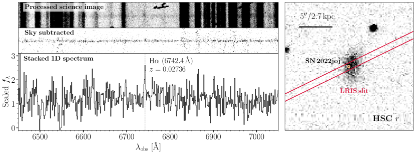
Figure 3: The LRIS spectrum reveals an H$\alpha$ emission line from the host galaxy at 6742.4 Å, corresponding to $z=0.02736$. Left: the H$\alpha$ emission in the observed 2D and 1D spectra. This emission line sits in the region free of strong night-sky lines and is unlikely due to bad sky subtraction. Right: image of the host galaxy and the position of SN 2022joj, with the orientation of the LRIS slit overplotted.

To determine the redshift of the host, we obtained two spectra about 300 days after the SN maximum brightness. On 2023 March 14, we took a spectrum of both the SN and the host using Binospec (Fabricant et al., 2019) on the 6.5 m MMT telescope with a total integration time of 5400 s. We placed the slit across both the center of the galaxy and the position of the SN (Figure 3). On 2023 April 26, we took another spectrum using the Low Resolution Imaging Spectrometer (LRIS; Oke et al., 1995) on the Keck I 10 m telescope. The slit was placed at the same position angle, with the Cassegrain Atmospheric Dispersion Compensator (Cass ADC; Phillips et al., 2006) module on. The total integration time was 3600 s. The LRIS spectrum has a higher signal-to-noise ratio (S/N), in which we detected a potential host emission line at 6742.4 Å (see Figure 3) with a S/N of 3.4. We associated this feature with H$\alpha$ emission, meaning the corresponding redshift of the host galaxy is $z=0.02736\pm 0.0007$, in agreement with the initial estimate, $z=0.03$, from matching the SN spectra to SNID templates (Newsome et al., 2022). In the coadded two-dimensional (2D) spectrum, the trace is dominated by the light of the SN in the nebular phase, while the center of this emission feature has an offset of $\sim$3–4 pixels from the center of the trace. The CCDs on LRIS have a scale of $0\farcs 135$ pixel^-1, so this offset corresponds to an angular offset of $\sim$$0\farcs 4$–$0\farcs 5$, consistent with the astrometric offset when comparing the LS detection of the host and the ZTF detection of the SN. The Binospec spectrum has a lower S/N, and we cannot identify this emission line at the same position in the 2D spectrum via visual inspection. Nevertheless, we still marginally detect an emission feature in the 1D spectrum with a S/N of 1.5 at the same wavelength. All the evidence indicates that the H$\alpha$ detection is real.

We estimate the distance modulus of SN 2022joj in the following way. We first use the 2M++ model (Carrick et al., 2015) to estimate the peculiar velocity of the host galaxy to be $244\pm 250$ $\mathrm{km}\,\mathrm{s}^{-1}$. Then the peculiar velocity is combined with the recession velocity in the frame of the cosmic microwave background (CMB) $v_{\mathrm{CMB}}=8424$ $\mathrm{km}\,\mathrm{s}^{-1}$, which yields a net Hubble recession rate of $8193\pm 250$ $\mathrm{km}\,\mathrm{s}^{-1}$. Using cosmological parameters $H_{0}=70\,\mathrm{km\,s^{-1}\,Mpc^{-1}}$, $\Omega_{M}=0.3$, and $\Omega_{\Lambda}=0.7$, the estimated luminosity distance to SN 2022joj is 119.5 Mpc, equivalent to a distance modulus of $35.39\pm 0.03$ mag.

Table 1: Host photometry of SN 2022joj.

Survey	Filter	$m$	$\sigma_{m}$
		(mag)	(mag)
HSC-SSP	PS $g$	$22.01$	$0.03$
HSC-SSP	PS $r$	$21.63$	$0.02$
HSC-SSP	PS $i$	$21.54$	$0.03$
HSC-SSP	PS $z$	$21.37$	$0.04$
HSC-SSP	PS $y$	$21.22$	$0.09$
LS	DECam $g$	$22.05$	$0.05$
LS	DECam $r$	$21.65$	$0.05$
LS	DECam $z$	$21.39$	$0.10$
LS	$W_{1}$	$21.94$	$0.35$

Note. — HSC-SSP – Hyper Suprime-Cam Subaru Strategic Program; LS – the DESI Legacy Imaging Survey; PS – Pan-STARRS; DECam – the Dark Energy Camera. All magnitudes are reported in the AB system (Oke & Gunn, 1983) and are not corrected for reddening.

2.3 Optical Photometry

SN 2022joj was monitored in ZTF $gri$ bands as part of its ongoing Northern Sky Survey (Bellm et al., 2019b). The $i_{\mathrm{ZTF}}$ data do not cover the rise. We use the forced-photometry light curves from ZFPS, reduced using the pipeline from A. A. Miller et al. (2023, in prep.); see also Yao et al. (2019). We adopt a Galactic extinction of ${E(B-V)_{\mathrm{MW}}}=0.032$ mag (Schlafly & Finkbeiner, 2011), and correct all photometry using the extinction model from Fitzpatrick (1999) assuming $R_{V}=3.1$. We do not find any Na I D absorption at the redshift of the host galaxy (we put a 3$\sigma$ upper limit in the equivalent width of Na I $\mathrm{D_{1}}+\mathrm{D_{2}}$ of $<$$0.5$ Å), indicating that the extinction from the host is negligible. The blue $g_{\mathrm{ZTF}}-r_{\mathrm{ZTF}}$ color ($\sim$$-0.2$ mag) near maximum luminosity after correcting for the Galactic extinction is also consistent with no additional reddening from the host. Therefore we assume ${E(B-V)}_{\mathrm{host}}=0$. The dereddened $g_{\mathrm{ZTF}}$ and $r_{\mathrm{ZTF}}$ forced-photometry light curves in absolute magnitudes are shown in Figure 1. Additional observations of SN 2022joj were obtained in the $o$ and $c$ filters in the ATLAS survey, the $griz$ filters with the optical imaging component of the Infrared-Optical suite of instruments (IO:O) on the Liverpool Telescope, the $griBVRI$ filters and the clear filter on the 0.76 m Katzman Automatic Imaging Telescope (KAIT; Filippenko et al., 2001) at Lick Observatory, and the $BVRI$ filters on the 1 m Anna Nickel telescope at Lick. ZTF, ATLAS, LT, KAIT, and Nickel observations are reported in Table 2. The ZTF $gri$ magnitudes, ATLAS $o$ and $c$ magnitudes, and Sloan $griz$ magnitudes are reported in the AB system, while the $BVRI$ and clear magnitudes are reported in the Vega system.

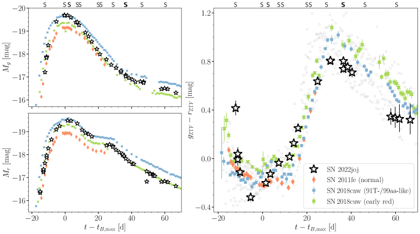
Figure 1: SN 2022joj (black stars) is an overluminous, fast-evolving SN Ia with a unique color evolution. In comparison, we show the photometric properties of SN 2011fe (normal SN Ia; Pereira et al., 2013), SN 2018cnw (91T-/99aa-like), and SN 2018cuw (normal SN Ia with a red early color). Left: multiband light curves. The upper (lower) panel shows the evolution in the $g$-band ($r$-band) absolute magnitude. Right: $g_{\mathrm{ZTF}}-r_{\mathrm{ZTF}}$ color evolution. The gray circles denote the color evolution of 14 nearby ($z\leq 0.05$) SNe Ia (open circles) from the ZTF sample with prompt observations within 5 days of first light (Bulla et al., 2020). The phases with respect to $t_{B,\mathrm{max}}$ (MJD 59722.77) are measured in the rest frame of the host galaxy. Correction for Galactic extinction has been applied, but $K$-corrections have not been performed. The epochs of optical spectroscopy are marked with “S” on the top axis.

2.4 Swift Ultraviolet/Optical Telescope (UVOT) Observations

Ultraviolet (UV) observations of SN 2022joj were obtained using UVOT (Roming et al., 2005) on the Neil Gehrels Swift Observatory (Swift; Gehrels et al., 2004) following a target-of-opportunity (ToO) request by E. Padilla Gonzalez. Prior to the SN, UVOT images of the field had been obtained in the $u$, $uvw1$, and $uvw2$ filters. In each of these reference images the flux at the location of the SN is consistent with 0, and the 3$\sigma$ upper limits correspond to $\lesssim$10% of the SN flux measured in the UV. In the optical bands, the LS photometry ($g=22.05\pm 0.05$ mag) shows that the host galaxy contributes $\lesssim$1% of the total observed flux. We therefore conclude that the host galaxy can be neglected when estimating the SN flux in UVOT images.

We determine the flux in the $u$, $b$, $v$, $uvw1$, $uvm2$, and $uvw2$ filters using a circular aperture with a radius of $5^{\prime\prime}$ centered at the position of the SN. To estimate the brightness of the sky background we use a coaxial annulus region with an inner/outer radius of $8^{\prime\prime}$/$15^{\prime\prime}$. The reduction is performed with the pipeline Swift_ToO based on the package HEAsoft version 6.30.1 (HEASARC, 2014). The magnitudes are also reported in Table 2 in the Vega system.

Table 2: Optical and UV Photometry of SN 2022joj.

$t_{\mathrm{obs}}$	Filter	$m$	$\sigma_{m}$	Magnitude	Telescope
(MJD)		(mag)	(mag)	System
59707.298	ZTF $r$	19.131	0.064	AB	P48/ZTF
59707.340	ZTF $r$	19.078	0.043	AB	P48/ZTF
59709.295	ZTF $r$	18.229	0.037	AB	P48/ZTF
59709.342	ZTF $r$	18.167	0.030	AB	P48/ZTF
59709.381	ZTF $r$	18.105	0.023	AB	P48/ZTF

Note. — Observed magnitudes in the ZTF, ATLAS, UVOT, LT, KAIT, and Nickel passbands. Correction for Galactic extinction has not been applied.

(This table is available in its entirety in machine readable form.)

2.5 Optical Spectroscopy

We obtained a series of optical spectra of SN 2022joj using the Spectral Energy Distribution Machine (SEDM; Blagorodnova et al., 2018) on the automated 60 inch telescope (P60; Cenko et al., 2006) at Palomar Observatory, the Kast double spectrograph (Miller & Stone, 1994) on the Shane 3 m telescope at Lick Observatory, the Andalucia Faint Object Spectrograph and Camera (ALFOSC) installed at the 2.56 m Nordic Optical Telescope (NOT), the SPectrograph for the Rapid Acquisition of Transients (SPRAT; Piascik et al., 2014) on the 2 m Liverpool Telescope (LT; Steele et al., 2004) under program PL22A13 (PI: Dimitriadis), the FLOYDS spectrograph on the 2 m Faulkes Telescope South (FTS) at Siding Spring as part of the Las Cumbres Observatory (LCO) (Brown et al., 2013), Binospec on the 6.5 m MMT telescope, and LRIS on the Keck I 10 m telescope. The SEDM spectra were reduced using the custom pysedm software package (Rigault et al., 2019). The Shane/Kast spectra, obtained with the slit near the parallactic angle to minimize differential slit losses (Filippenko, 1982), were reduced following standard techniques for CCD processing and spectrum extraction (Silverman et al., 2012) utilizing IRAF (Tody, 1986) routines and custom Python and IDL codes. The NOT/ALFOSC, Keck I/LRIS, and MMT/Binospec spectra were reduced using the PypeIt package (Prochaska et al., 2020). The LT/SPRAT spectra were reduced with a dedicated pipeline for bias subtraction, flat fielding, derivation of the wavelength solution and flux calibration, with additional IRAF/PyRAF routines for proper extraction of the spectra. The FTS/FLOYDS spectrum was reduced using the FLOYDS pipeline. We also attempted to obtain a near-infrared spectrum with the Triple Spectrograph (TSpec) installed at the 200 inch Hale telescope (P200; Oke & Gunn, 1982) at Palomar observatory, but the observations are mostly characterized by low S/N and a few broad undulations with no immediately identifiable lines. Thus, the TSpec data were excluded from our analysis. Details of the spectroscopic observations are listed in Table 3. The resulting spectral sequence is shown in Figure 2. All of the spectra listed in Table 3 will be available on WISeREP (Yaron & Gal-Yam, 2012).

We also include the spectrum uploaded to the Transient Name Server (TNS) by Newsome et al. (2022) in our analysis, which was obtained using the FLOYDS spectrograph on the 2 m Faulkes Telescope North (FTN) at Haleakala.

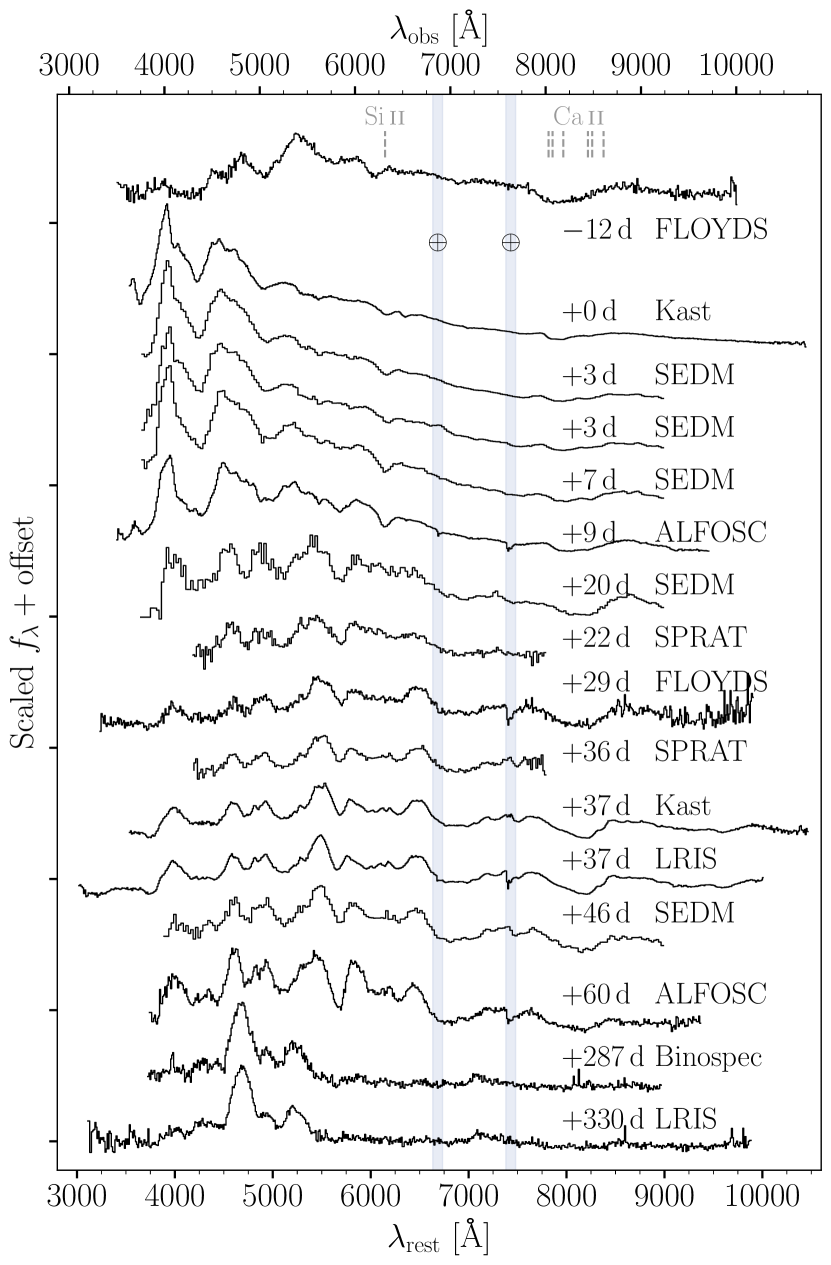
Figure 2: Optical spectral sequence of SN 2022joj showing the red to blue color transition as the SN rises to its maximum luminosity and the development of prominent absorption features around 4200 Å post-maximum. Rest-frame phase relative to the $B$-band peak and the instrument used to observe the SN are listed for each spectrum. Spectra have been corrected for ${E(B-V)_{\mathrm{MW}}}=0.032$ mag. All spectra are binned with a bin size of 10 Å, except for the low-resolution SEDM spectra. The corresponding wavelengths of the Si II $\lambda$6355 line (with an expansion velocity of 10,000 $\mathrm{km}\,\mathrm{s}^{-1}$) and the Ca II IRT (with expansion velocities of both 10,000 $\mathrm{km}\,\mathrm{s}^{-1}$ and 25,000 $\mathrm{km}\,\mathrm{s}^{-1}$) are marked by the vertical dashed lines. The strong optical telluric features (Fraunhofer A and B bands) are marked by the shaded region.

Table 3: Spectroscopic observations of SN 2022joj.

$t_{\mathrm{obs}}$	Phase	Telescope/	$R$	Range
(MJD)	(days)	Instrument	$(\lambda/\Delta\lambda)$	(Å)
59,710.29	$-$12.1	FTN/FLOYDS-N	550	3500–10000
59,722.43	$-$0.3	Shane/Kast	750	3630–10730
59,725.34	$+$2.6	P60/SEDM	100	3770–9220
59,725.43	$+$2.6	P60/SEDM	100	3770–9220
59,730.27	$+$7.4	P60/SEDM	100	3770–9220
59,732.02	$+$9.0	NOT/ALFOSC	360	3500–9700
59,743.28	$+$20.0	P60/SEDM	100	3770–9220
59,744.24	$+$20.9	P200/TSpec	2500	10000–24630
59,744.96	$+$21.6	LT/SPRAT	350	4020–7990
59,752.50	$+$29.0	FTS/FLOYDS-S	550	3500–10000
59,759.92	$+$36.2	LT/SPRAT	350	4020–7990
59,760.28	$+$36.5	Shane/Kast	750	3630–10750
59,760.37	$+$36.7	Keck I/LRIS	1100	3100–10280
59,770.25	$+$46.3	P60/SEDM	100	3770–9220
59,784.89	$+$60.5	NOT/ALFOSC	280	3850–9620
60,017.42	$+$286.9	MMT/Binospec	1340	3830–9210
60,061.56	$+$329.8	Keck I/LRIS	1100	3200–10150

Note. — Phase is measured relative to the $B$-band peak in the rest frame of the host galaxy. The resolution $R$ is reported for the central region of the spectrum.

3 Analysis

3.1 Early Light Curves and the First Light

To estimate the time of first light ($t_{\mathrm{fl}}$), we assume an initial power-law rise in the broad-band flux $f(t)$,

$$f(t)=A(t-t_{\mathrm{fl}})^{\alpha},$$

where $A$ is a constant and $\alpha$ is the power-law index. We only include the forced-photometry light curve with flux $\leq$40% of peak luminosity (Miller et al., 2020) in $r_{\mathrm{ZTF}}$ and ATLAS $o$, in which observations were conducted on more than three nights between $-20$ days and $-10$ days. Light curves in other bands are excluded because the coverage is significantly worse at this phase (see Section 3.2). We assume that the $t_{\mathrm{fl}}$ is the same in both bands, then estimate $\alpha$ and $A$ in each band with a Bayesian approach. We adopt flat priors for $t_{\mathrm{fl}}$ and $\log A$, and a normal prior for each $\alpha$ centered at 2 (the fireball model) with a standard deviation of 1. We sample their posterior distributions with Markov Chain Monte Carlo (MCMC) using the package PyMC (Salvatier et al., 2016). In addition, we run another model with a fixed $\alpha=2$. The estimated model parameters are listed in Table 4. We find that both light curves are consistent with a power-law rise since MJD $59703.16^{+0.70}_{-0.58}$. This estimate is consistent with the $\alpha=2$ fireball model. When fixing $\alpha=2$, the model also fits the light curve well, but the estimated $t_{\mathrm{fl}}$ is $\sim$0.5 day later (MJD $59703.66_{-0.11}^{+0.10}$). We do not find any correlated residuals as evidence for a flux excess after $\sim$4 days since $t_{\mathrm{fl}}$, although a flux excess before the first detection could not be ruled out.

3.2 Photometric Properties

The basic photometric properties of SN 2022joj are listed in Table 4. The times of the maximum luminosity and the corresponding magnitudes in the ZTF $gr$ bands and the KAIT/Nickel $BVRI$ bands are estimated using a fourth-order polynomial fit. We do not include the maximum $i_{\mathrm{ZTF}}$-band properties, which are relatively uncertain owing to the low cadence in $i_{\mathrm{ZTF}}$ around peak.

SN 2022joj shows a few peculiar photometric features compared to normal SNe Ia. In Figure 1, we compare the $g_{\mathrm{ZTF}}$ and $r_{\mathrm{ZTF}}$ light curves and the $g_{\mathrm{ZTF}}-r_{\mathrm{ZTF}}$ color evolution of SN 2022joj with those of the well-observed normal SN Ia, SN 2011fe, as well as SN 2018cnw (ZTF18abauprj) and SN 2018cuw (ZTF18abcflnz) from a sample of SNe Ia with prompt observations within 5 days of first light by ZTF (Yao et al., 2019; Bulla et al., 2020). SN 2018cnw is slightly overluminous at peak, and belongs to either the SN 1999aa-like (99aa-like; Garavini et al., 2004) or SN 1991T-like (91T-like; Filippenko et al., 1992a) subclass of SNe Ia, while SN 2018cuw is a normal SN Ia with a red $g_{\mathrm{ZTF}}-r_{\mathrm{ZTF}}$ color comparable to that of SN 2022joj $\sim$15 days prior to peak.

Around maximum brightness, SN 2022joj is overluminous, comparable to SN 2018cnw, and $\sim$0.5 mag brighter than SN 2011fe in both $g_{\mathrm{ZTF}}$ and $r_{\mathrm{ZTF}}$. But SN 2022joj clearly stands out owing to its fast evolution in $g_{\mathrm{ZTF}}$. While SN 2022joj and SN 2018cnw show a similar maximum brightness in $g_{\mathrm{ZTF}}$, upon the first detection of SN 2022joj in $g_{\mathrm{ZTF}}$ at $\sim$$-12$ days, its corresponding absolute magnitude ($-17.2$ mag) is $\sim$0.8 mag fainter than that of SN 2018cnw at a similar phase. This means on average, SN 2022joj rises faster than SN 2018cnw by $\sim$$0.06\,\mathrm{mag\,day^{-1}}$ in $g_{\mathrm{ZTF}}$ during that period of time. On the decline, the $\Delta m_{15}(g_{\mathrm{ZTF}})$ of SN 2022joj is $1.03\pm 0.03$ mag, which is significantly greater than that of the overluminous SN 2018cnw ($\Delta m_{15}(g_{\mathrm{ZTF}})=0.77$ mag) or normal SN 2011fe ($\Delta m_{15}(g_{\mathrm{ZTF}})=0.80$ mag). The rapid decline of SN 2022joj is atypical for overluminous SNe Ia, which are usually the slowest decliners in the SN Ia population (Phillips et al., 1999; Taubenberger, 2017). The rapid decline is probably due to the unusual and fast-developing absorption feature near 4200 Å (see Section 3.3).

The color evolution of SN 2022joj does not match that of normal SNe Ia, as shown by the trail traced by SN 2022joj in the right panel of Figure 1. We overplot all the SNe from the ZTF early SN Ia sample (Bulla et al., 2020) with $z\leq 0.05$. They are corrected for Galactic extinction, but $K$-corrections have not been performed for consistency. Given the peculiar nature of SN 2022joj, we cannot use models trained on normal SNe Ia to reliably estimate its $K$-correction. Nevertheless, given its relatively low redshift ($z\lesssim 0.03$), the $K$-corrections are not expected to be large ($K(g_{\mathrm{ZTF}}-r_{\mathrm{ZTF}})\simeq-0.05$ mag around maximum, estimated using the Kast spectrum at $-0.3$ days). For the same reason we only include the SNe Ia with the lowest redshift from the sample of Bulla et al. (2020). SN 2022joj is remarkably red ($g_{\mathrm{ZTF}}-r_{\mathrm{ZTF}}\simeq 0.4$ mag) at $\sim$$-12$ days ($\sim$7 days after $t_{\mathrm{fl}}$), and is clearly an outlier compared to the normal SN Ia sample. During the ensuing week, SN 2022joj quickly evolves to the blue, and is among the bluest objects in the sample at $\sim$$-5$ days ($\sim$14 days after $t_{\mathrm{fl}}$; $g_{\mathrm{ZTF}}-r_{\mathrm{ZTF}}\simeq-0.3$ mag). SN 2018cuw has a comparable $g_{\mathrm{ZTF}}-r_{\mathrm{ZTF}}$ color at early times, but the blueward evolution of SN 2018cuw is slower than that of SN 2022joj. No later than SN 2022joj reaches its peak luminosity, SN 2022joj starts to evolve redward. While other SNe Ia show qualitatively similar redward evolution, this usually happens much later ($\sim$$+10$ days). When $g_{\mathrm{ZTF}}-r_{\mathrm{ZTF}}$ reaches maximum ($\sim$0.8 mag) at $\sim$$+30$ days, SN 2022joj is again bluer than most of the SNe Ia in the ZTF sample. Eventually as SN 2022joj steps into the transitional phase, its color evolution follows the Lira law (Lira, 1996; Phillips et al., 1999) and shows no significant difference from that of the SNe Ia in the ZTF sample. The $B-V$ color evolves in the similar way as the $g_{\mathrm{ZTF}}-r_{\mathrm{ZTF}}$ color, which starts red ($B-V\simeq 1.2$ mag at $-12$ days) and quickly turns bluer, reaching $B-V\simeq 0.0$ mag at $\sim$$-5$ days before turning red again.

While SN 2022joj shows a blue $g_{\mathrm{ZTF}}-r_{\mathrm{ZTF}}$ color near maximum brightness, its UV $-$ optical colors are unusually red. In Figure 4, we show the locations of SN 2022joj in the UVOT color-color diagrams compared to those of 29 normal SNe Ia with UV observations around maximum from Brown et al. (2018). SN 2022joj stands out due to the red $u-v$ and $uvw1-v$ colors. After correcting for Galactic extinction, SN 2022joj shows $u-v=0.58^{+0.06}_{-0.06}$ mag and $uvw1-v=2.48^{+0.23}_{-0.19}$ mag. As a comparison, none of the objects in the normal SN Ia sample has $u-v>0.5$ mag or $uvw1-v>2.1$ mag. This cannot be a result of the unknown host reddening, since the amount of host extinction needed to account for the red near-UV colors of SN 2022joj would require the intrinsic $b-v$ color of the SN to be unphysically blue (shifted along the opposite direction of the arrows in Figure 4). Interestingly, SN 2022joj exhibits a moderately blue mid-UV color ($uvm2-uvw1=1.59^{+0.55}_{-0.36}$ mag), while most of the normal SNe Ia in the sample from Brown et al. (2018) show $uvm2-uvw1\gtrsim 2$ mag. This might indicate that, for some reason, the flux in the near-UV ($\sim$2500–4000 Å) of SN 2022joj is suppressed near maximum brightness.

To conclude, despite a similar luminosity and color to 99aa-like/91T-like events at maximum brightness, the rapid photometric rise and decline and the unusual color evolution in SN 2022joj both indicate that it exhibits some peculiarities relative to normal and 99aa-like/91T-like SNe Ia.

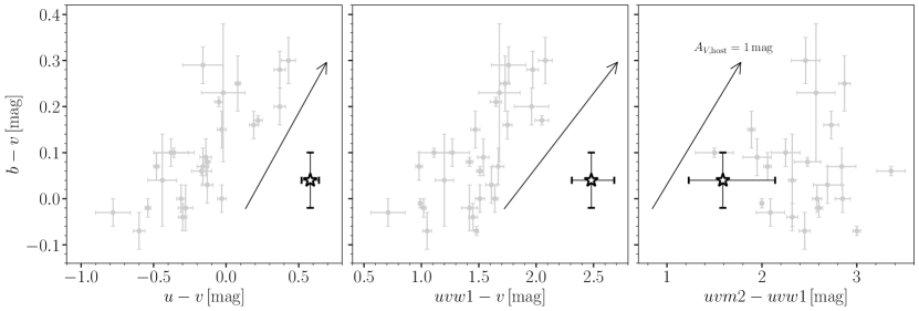
Figure 4: The color-color diagrams using UVOT photometry show that SN 2022joj (black star) has very unusual UV$-$optical colors at maximum luminosity compared to normal SNe Ia (gray dots; a sample of 29 normal SNe Ia from Brown et al., 2018). The arrows mark how SN 2022joj would move in each color-color space if there were host reddening with the visual extinction of $A_{V,\mathrm{host}}=1$ (assuming $R_{V}=3.1$).

Table 4: Basic photometric properties of SN 2022joj.

Rise (flux $\leq$$40\%$ of peak luminosity)
Variable $\alpha$: prior – $N(2,1)$				Fixed $\alpha$: $\alpha=2$
$t_{\mathrm{fl}}$ (MJD)	$\alpha_{\mathrm{ZTF},r}$	$\alpha_{\mathrm{ATLAS},o}$		$t_{\mathrm{fl},\alpha=2}$ (MJD)
$59703.16^{+0.70}_{-0.58}$	$2.18^{+0.20}_{-0.24}$	$2.37^{+0.48}_{-0.20}$		$59703.66^{+0.10}_{-0.11}$
Maximum luminosity
Filters	$g_{\mathrm{ZTF}}$	$r_{\mathrm{ZTF}}$	$B$	$V$	$R$	$I$
$t_{\mathrm{max,poly}}$ (MJD)	$59722.66\pm 0.21$	$59725.54\pm 0.09$	$59722.77\pm 0.30$	$59724.88\pm 0.28$	$59724.61\pm 0.28$	$59720.73\pm 0.27$
$M_{\mathrm{max,poly}}$ (mag)	$-19.693\pm 0.014$	$-19.492\pm 0.004$	$-19.456\pm 0.011$	$-19.544\pm 0.009$	$-19.496\pm 0.009$	$-19.222\pm 0.011$

Note. — Parameters are defined in the text. The absolute magnitudes have been corrected for Galactic extinction. The uncertainty in the distance modulus (0.03 mag) and the systematics in the polynomial models are not included.

3.3 Optical Spectral Properties

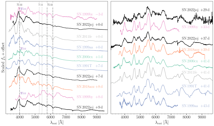
Figure 5: Optical spectra of SN 2022joj (black) and (i) a subluminous SN Ia, SN 1999by (magenta), (ii) a normal SN Ia, SN 2011fe (gray), (iii) two overluminous SNe Ia, SN 1991T and SN 1999aa (blue), (iv) the peculiar SN 2000cx (green), and (v) a normal SN Ia with a red color at early times, SN 2018aoz (orange), near maximum brightness (left panel) and about a month after maximum (right panel). The dash-dotted lines correspond to wavelengths of three Si II lines (4128 Å, 5972 Å, and 6355 Å), while the dotted lines correspond to the wavelengths of the S II “W-trough” (both assuming an expansion velocity of 10,000 $\mathrm{km}\,\mathrm{s}^{-1}$). Ti II has been identified from the spectra of SN 1999by and SN 2000cx at around $\sim$4200 Å, and the corresponding features are labeled. Spectra were downloaded from WiseREP (Yaron & Gal-Yam, 2012), with the following original data sources: SN 2011fe – Pereira et al. (2013); Mazzali et al. (2014); SN 1991T, SN 1999aa, and SN 2000cx – Silverman et al. (2012); SN 1999by – Matheson et al. (2008); SN 2018aoz – Ni et al. (2023).

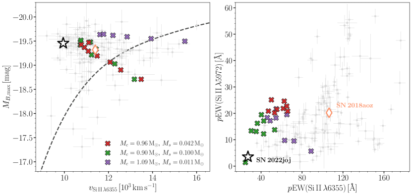
Figure 6: SN 2022joj (black star) is an SN Ia showing a normal brightness in $B$ and remarkably shallow Si II features with a relatively low expansion velocity at maximum luminosity, compared to a sample of normal SNe Ia (gray dots) from Zheng et al. (2018) and Burrow et al. (2020). Left: the $B$-band absolute magnitude vs. the expansion velocity of Si II $\lambda$6355 at maximum brightness. Right: the pseudo-equivalent widths ($p$EWs) of the two Si II lines, Si II $\lambda\lambda$5972, 6355, at maximum brightness. The dashed black line corresponds to the theoretical $M_{B,\mathrm{max}}$-$v_{\mathrm{Si\,\textsc{ii}}}$ relation of 1D double-detonation models for thin helium shells across a spectrum of progenitor masses in Polin et al. (2019). The colored $\times$ symbols show 2D double-detonation models from Shen et al. (2021b) with different C/O core mass ($M_{c}$) and helium shell mass ($M_{s}$), and viewing angles. For each model, multiple symbols are shown to summarize the effect of different viewing angles, from $\mu=-0.93$ to $\mu=+0.93$ ($\mu$ defined as the cosine of the polar angle relative to the point where the helium-shell detonation occurs). Parameters of the candidate double-detonation normal SN Ia, SN 2018aoz (Ni et al., 2023), are also overplotted as an orange diamond.

In Figure 2, we show the optical spectral sequence of SN 2022joj. The $-12$ days spectrum exhibits prominent absorption lines associated with Si II $\lambda$6355 and Ca II IRT (this spectrum was obtained and posted on TNS by Newsome et al. 2022). It also displays a strong suppression of flux blueward of $\sim$5000 Å, confirming the unusually red photometric colors at early times. Near maximum brightness, the Kast spectrum and the two SEDM spectra show a very blue continuum in the range $\sim$5000–8000 Å with shallow absorption features, indicating a high photometric temperature. Si II $\lambda\lambda$5972, 6355 lines, the S II W-trough, and Ca II IRT are detectable but not prominent. The C II $\lambda\lambda$6580, 7234 lines are prominent at maximum brightness ($+0$ day), and quickly disappear afterward ($+3$ days). A wide, asymmetric absorption feature appears at $\sim$4000–4500 Å (the 4200 Å features hereafter). There is a break on the blue edge of this feature which we associate with Si II $\lambda$4128 that is often seen in other SNe Ia. The 4200 Å features become even wider and deeper in another SEDM spectrum at $+7$ days and the ALFOSC spectrum at $+9$ days. Weeks after the maximum, in the FLOYDS spectrum ($+29$ days) and the LRIS spectrum ($+36$ days), the bottom of the 4200 Å features becomes flat, reminiscent of the Ti-trough in the subluminous SN 1991bg-like (91bg-like; Filippenko et al., 1992b; Leibundgut et al., 1993) SNe. The nebular-phase spectra are dominated by [Fe II] and [Fe III] emission lines, but the [Fe II] features (e.g, the complex around $\sim$7300 Å) are weaker than in other SNe Ia (Figure 9), suggesting that the ejecta remain highly ionized about a year after the explosion. The nebular spectra are discussed in detail in Section 4.2.

In Figure 5, we compare maximum-light and transition-phase spectra of SN 2022joj to those seen in other SNe Ia. Around peak, the blue continuum and shallow absorption features in SN 2022joj are similar to those of overluminous objects, including SN 1991T, SN 1999aa, and SN 2000cx. The asymmetric 4200 Å features are not seen in normal (SN 2011fe) or overluminous (SN 1991T and SN 1999aa) SNe Ia, which all show another maximum at $\sim$4100 Å redward of the narrow Si II $\lambda$4128 feature. In SN 2000cx, a similar (but narrower) absorption feature is interpreted as high-velocity Ti II (Branch et al., 2004). The 4200 Å features are actually much more similar to the well-known “Ti-trough” that is ubiquitous in subluminous 91bg-like objects, e.g., SN 1999by (Arbour et al., 1999). Prior to the peak, SN 1999by also shows this asymmetric absorption at about the same wavelength, which becomes more prominent with a nearly flat-bottom trough about a week after maximum. This absorption is caused by a blend of multiple species dominated by Ti II (Filippenko et al., 1992b; Mazzali et al., 1997). It remains prominent in the spectrum up to one month after maximum. Similarly, we find similar features in the spectra of SN 2022joj at $+29$ days and $+36$ days. Other normal/overluminous SNe Ia, unlike SN 2022joj, all exhibit a dip around $\sim$4500 Å. Aside from the 4200 Å features, SN 2022joj is otherwise entirely dissimilar from 91bg-like objects, which are $\gtrsim$2 mag fainter at peak and exhibit much stronger Si II, Ca II and O I absorption from a cooler line-forming region (Filippenko et al., 1992b). The Ti-trough in 91bg-like SNe is interpreted as the result of a low photospheric temperature (Mazzali et al., 1997).

SN 2022joj also shows remarkably shallow Si II absorption at maximum brightness. Following the techniques elaborated in Liu et al. (2023a) (see also Childress et al., 2013, 2014; Maguire et al., 2014), we fit the Si II and Ca II IRT features with multiple Gaussian profiles. We find that modeling the Ca II IRT absorption requires two distinct velocity components — the photospheric-velocity features (PVFs) and the high-velocity features (HVFs). In Table 5 we list the estimates of the expansion velocities and the pseudo-equivalent widths ($p$EWs) of the major absorption lines from $-12$ days to $+9$ days. In Figure 6 we show the peak absolute magnitude in $B$ band ($M_{B,\mathrm{max}}$) vs. the velocity and $p$EW of Si II for SN 2022joj and a sample of normal SNe Ia from Zheng et al. (2018) and Burrow et al. (2020). Figure 6 highlights that SN 2022joj has a normal $M_{B,\mathrm{max}}$ with a relatively low Si II $\lambda$6355 expansion velocity (hereafter $v_{\mathrm{Si\,\textsc{ii}}}$). The Si II $\lambda$5972 and Si II $\lambda$6355 $p$EWs in SN 2022joj are lower than that for most normal SNe Ia. In fact, SN 2022joj sits at the extreme edge of the shallow-silicon group proposed in Branch et al. (2006), which mainly consists of overluminous 91T-like/99aa-like objects. This is consistent with the high luminosity and the blue color of SN 2022joj at maximum light, since a high photometric temperature results in higher ionization, reducing the abundance of singly ionized atoms (e.g., Si II). Interestingly, the $p$EW of Si II $\lambda$6355 near peak is significantly lower than that in the first spectrum. In typical 91T-like/99aa-like objects, the Si II features are weak or undetectable at early times because the ejecta are even hotter, and only start to emerge around maximum light (Filippenko et al., 1992a). In the early spectrum of SN 2022joj, in contrast, stronger absorption features from singly ionized Si and Ca indicate a cooler line-forming region at early times compared to that at maximum brightness.

Prominent C II features are also detected in the overluminous SN 2003fg-like (03fg-like; Howell et al., 2006) SNe at their maximum brightness. However, 03fg-like objects show blue colors in the early light curves (Taubenberger et al., 2019) and appear even brighter in near-UV compared to normal SNe Ia at peak (Brown et al., 2014), dissimilar from that of SN 2022joj. Many 03fg-like objects also show strong oxygen features both in their maximum-light and late-time spectra (Taubenberger et al., 2019), while in SN 2022joj, we do not find evidence for oxygen. Consequently, the explosion mechanism as well as the origin of carbon in SN 2022joj is likely very different from that of 03fg-like objects.

In conclusion, the spectral evolution of SN 2022joj shows some similarities to 91T-like/99aa-like objects, as well as peculiarities. A reasonable model to explain SN 2022joj needs to reproduce (i) a strong suppression in flux blueward of $\sim$5000 Å at early times followed by a rapid evolution to blue colors; (ii) the seemingly contradictory observables at peak, namely the 4200 Å features similar to the Ti-trough in 91bg-like objects and the blue continuum/shallow Si II feature at maximum, which separately indicate low and high photometric temperatures, respectively; and (iii) prominent C II features at maximum brightness.

Table 5: Fits to the expansion velocities and pEWs of Si II $\lambda\lambda$5972, 6355 and the Ca II IRT of SN 2022joj.

	Si II $\lambda$5972		Si II $\lambda$6355		Ca II IRT, PVFs		Ca II IRT, HVFs
Phase	$v$	$p$EW	$v$	$p$EW	$v$	$p$EW	$v$	$p$EW
(day)	($10^{3}$ $\mathrm{km}\,\mathrm{s}^{-1}$)	(Å)	($10^{3}$ $\mathrm{km}\,\mathrm{s}^{-1}$)	(Å)	($10^{3}$ $\mathrm{km}\,\mathrm{s}^{-1}$)	(Å)	($10^{3}$ $\mathrm{km}\,\mathrm{s}^{-1}$)	(Å)
$-12.1$	$\cdots$	$\cdots$	$-15.66\pm 0.13$	$47.5\pm 2.5$	$-14.85\pm 0.83$	$190\pm 34$	$-25.98\pm 0.56$	$278\pm 40$
$-0.3$	$-10.10\pm 0.88$	$3.5\pm 1.9$	$-9.95\pm 0.07$	$27.2\pm 0.8$	$-12.45\pm 0.17$	$58\pm 2$	$-23.35\pm 0.06$	$117\pm 2$
$+2.5$	$-8.77\pm 0.63$	$2.9\pm 1.5$	$-10.28\pm 0.13$	$27.8\pm 1.3$	$-12.03\pm 0.73$	$58\pm 11$	$-22.51\pm 0.33$	$109\pm 11$
$+2.6$	$-8.35\pm 0.62$	$4.4\pm 2.6$	$-9.87\pm 0.28$	$25.4\pm 2.7$	$-11.77\pm 0.93$	$85\pm 17$	$-22.17\pm 0.47$	$105\pm 15$
$+7.3$	$\cdots$	$\cdots$	$-10.52\pm 0.17$	$40.9\pm 2.7$	$-10.10\pm 0.82$	$79\pm 18$	$-20.88\pm 0.57$	$172\pm 24$
$+9.0$	$\cdots$	$\cdots$	$-10.37\pm 0.04$	$48.5\pm 0.6$	$-11.94\pm 0.23$	$144\pm 6$	$-21.13\pm 0.15$	$127\pm 6$

3.4 Host-Galaxy Properties

We model the observed spectral energy distribution (SED; photometry in HSC-SSP $grizy$ and LS $W_{1}$ filters) with the software package Prospector version 1.1 (Johnson et al., 2021). The LS $grz$ photometry, which is consistent with the HSC-SSP results but has a lower S/N, is excluded from this modeling. We assume a Chabrier initial-mass function (IMF; Chabrier, 2003) and approximate the star-formation history (SFH) by a linearly increasing SFH at early times followed by an exponential decline at late times (functional form $t\times\exp\left(-t/\tau\right)$, where $t$ is the age of the SFH episode and $\tau$ is the $e$-folding timescale). The model is attenuated with the Calzetti et al. (2000) model. The priors of the model parameters are set identically to those used by Schulze et al. (2021).

The SED is adequately described by a galaxy template with a mass of $\log(M_{*}/\mathrm{M_{\odot}})=7.13^{+0.15}_{-0.28}$, suggesting that the host is a dwarf galaxy. The modeled star-formation rate (SFR) is consistent with 0, but we note that measuring low SFRs with SED fitting is not robust and subject to systematics (Conroy, 2013). In addition, the H$\alpha$ emission detected in the late-time spectrum of the SN (Section 2.2) indicates at least some level of star formation in the host.

4 Discussion

4.1 SN 2022joj Compared to Model Explosions

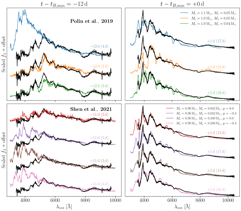
Figure 7: Comparisons of an early spectrum ($-12$ days) and a maximum-light spectrum ($+0$ days) of SN 2022joj (black) with two sets of double-detonation models. For each synthetic spectrum, the phase relative to $t_{B,\mathrm{max}}$ is listed (the time since explosion is shown in parentheses). Top: comparison with 1D models from Polin et al. (2019) with different C/O core ($M_{c}$) and He shell ($M_{s}$) masses. Bottom: comparison with 2D models from Shen et al. (2021b) with different masses and viewing angles $\mu$. The observed spectra have been corrected for Galactic extinction.

There are several physical mechanisms that can produce blue colors during the early evolution of SNe Ia, including heating of the SN ejecta following the decay of radioactive ⁵⁶Ni, interaction of the SN ejecta with a nondegenerate companion (e.g., Kasen, 2010), collisions between the SN ejecta and circumstellar material (e.g., Piro & Morozova, 2016), strong mixing that surfaces ⁵⁶Ni to the outermost layers of the ejecta (e.g., Piro & Nakar, 2013; Magee & Maguire, 2020), and/or the production of radioactive isotopes in the detonation of a helium shell on the surface of the exploding WD (e.g., Noebauer et al., 2017; Polin et al., 2019).

In contrast, there are few proposed scenarios that can produce red colors up to a week after explosion, as in the case of SN 2022joj. If the newly synthesized ⁵⁶Ni is strongly confined to the innermost SN ejecta, then an SN may remain red for several days after explosion as the heating diffuses out toward the photosphere (Piro & Morozova, 2016). Even the most confined ⁵⁶Ni configuration considered in Piro & Morozova (2016) converges to blue colors, similar to explosions with more extended ⁵⁶Ni distributions, within $\sim$6 days after explosion. SN 2022joj is observed to have very red colors $\sim$7 days after $t_{\mathrm{fl}}$ (meaning more than 7 days after explosion, since SNe Ia have a “dark phase” before photons diffuse out of the ejecta; Piro & Nakar 2013). Dessart et al. (2014) considered more realistic delayed-detonation scenarios. Some of their 1D unmixed delayed-detonation models still show a red $B-R$ color ($B-R\gtrsim 0.5$ mag) 7 days after the explosion (see the DDC20, DDC22, and DDC25 models in their Figure 1), comparable to that of SN 2022joj. However, these models never appear as blue as SN 2022joj at peak ($B-R\simeq 0.0$ mag), and the ⁵⁶Ni yields are relatively low ($M_{\mathrm{Ni56}}\lesssim 0.3\,\mathrm{M_{\odot}}$), so they would result in subluminous events. In addition, we do not know any multidimensional explosion models that fail to produce any ⁵⁶Ni mixing within the ejecta, and therefore disfavor this scenario.

Alternatively, in the double-detonation scenario, a layer of IGEs in the ashes of the helium shell can produce significant opacity in the outer layers of the bulk ejecta, producing a red color (Polin et al., 2019). This scenario has been proposed for a few normal-luminosity SNe with red colors at early times, including SN 2016jhr (Jiang et al., 2017) and SN 2018aoz (Ni et al., 2022). In Figure 7 we compare the spectra of SN 2022joj at $-12$ days and $+0$ day with 1D double-detonation models from Polin et al. (2019) and 2D double-detonation models from Shen et al. (2021b). To create synthetic spectra, both models use Sedona (Kasen et al., 2006), a multi-dimensional radiative transfer (RT) simulator that assumes local thermodynamical equilibrium (LTE).

In the 1D models, the most important parameters are the mass of the C/O core ($M_{c}$) and the mass of the helium shell ($M_{s}$). The maximum luminosity depends on the amount of ⁵⁶Ni synthesized in the explosion, which is predominantly determined by the total progenitor mass ($M_{c}+M_{s}$; Polin et al., 2019). We find that the maximum brightness in $B$ band ($M_{B,\mathrm{max}}=-19.46$ mag) is reproduced by the 1D models with relatively massive progenitors ($\sim$1.1 $\mathrm{M_{\odot}}$). However, models with such massive progenitors tend to produce blue, featureless spectra at early times (e.g., the $M_{c}=1.1\,\mathrm{M_{\odot}}$, $M_{s}=0.05\,\mathrm{M_{\odot}}$ model in Figure 7), inconsistent with the observations. Less-massive models provide a better match to the line-blanketing seen in the early spectra, but fail to reproduce the maximum brightness as well as the 4200 Å features in the observed spectra. The 1D models overestimate the $p$EW and the expansion velocity of the Si II $\lambda$6355 line at peak. As a reference, we overplot the theoretical $M_{B,\mathrm{max}}$-$v_{\mathrm{Si\,\textsc{ii}}}$ relation of 1D double-detonation models for thin helium shells ($M_{s}\simeq 0.01\,M_{\odot}$) across a spectrum of progenitor masses in Polin et al. (2019) as the dashed black curve in the left panel of Figure 6, which is not in agreement with the properties of SN 2022joj. Besides, none of the models produce detectable C II features in the spectra at peak.

While the 1D models do not fully reproduce the observed properties of SN 2022joj, some of these tensions can be resolved when considering viewing-angle effects in multi-dimensional models. In Figure 6 we also show the properties of three 2D double-detonation models from Shen et al. (2021b) with a variety of $M_{c}$ and $M_{s}$. For consistency in comparing the synthetic brightness with the observations of SN 2022joj, of which the $K$-corrections are unknown, the synthetic fluxes in the $B$ filter of these models are evaluated after shifting the synthetic spectra to $z=0.02736$, the redshift of SN 2022joj. We obtain the Si II line properties using the same fitting techniques as in Section 3.3. We again find that more-massive progenitors generally lead to higher-luminosity SNe, but different viewing angles produce significantly different spectral properties as a result of the asymmetry of the ejecta — materials closer to the point of helium ignition are less dense and expand faster (Shen et al., 2021b). In the plot, the cosine value of the polar angle relative to the point of helium ignition, $\mu$, ranges from $+0.93$ (near the helium ignition point) to $-0.93$ (opposite to the helium ignition point). When the SN is observed along a line of sight closer to the detonation point in the shell (greater $\mu$), it will appear fainter at maximum brightness and show a higher line velocity in Si II $\lambda$6355. For a relatively high progenitor mass ($\gtrsim$$1.1\,\mathrm{M_{\odot}}$), a high $v_{\mathrm{Si\,\textsc{ii}}}$ ($\gtrsim$$13,500$ $\mathrm{km}\,\mathrm{s}^{-1}$) is predicted in 1D models. However, all of the 2D models with $\mu\lesssim 0$ show a lower $v_{\mathrm{Si\,\textsc{ii}}}$ ($\lesssim$$12,000$ $\mathrm{km}\,\mathrm{s}^{-1}$), much closer to SN 2022joj in the $M_{B,\mathrm{max}}$-$v_{\mathrm{Si\,\textsc{ii}}}$ phase space. Models with $\mu>0$ are more consistent with 1D model predictions. It is suggested by Polin et al. (2019) that high-velocity SNe that follow the dashed line in Figure 6 result from sub-$M_{\mathrm{Ch}}$ double detonations, while SNe in the clump centered at $M_{B,\mathrm{max}}\simeq-19.5$ mag and $v_{\mathrm{Si\,\textsc{ii}}}\simeq 11,000$ $\mathrm{km}\,\mathrm{s}^{-1}$ are likely near-$M_{\mathrm{Ch}}$ explosions. Based on the 2D models, however, we should expect a similar number of high-velocity and normal-velocity double-detonation SNe Ia. A substantial fraction of the objects within the clump on the $M_{B,\mathrm{max}}$-$v_{\mathrm{Si\,\textsc{ii}}}$ diagram may be sub-$M_{\mathrm{Ch}}$ double-detonation events viewed from certain orientations (Shen et al., 2021b). SN 2018aoz is a double-detonation candidate that, like SN 2022joj, exhibits early red colors before evolving to normal luminosity and blue colors (Ni et al., 2022). Interestingly, SN 2018aoz also resides in the high-luminosity, low-velocity clump in the $M_{B,\mathrm{max}}$-$v_{\mathrm{Si\,\textsc{ii}}}$ space (Ni et al., 2023), and thus, it too may be an example of a double-detonation SN Ia viewed from the hemisphere opposite to the helium ignition point.

In the bottom panels of Figure 7 we show two 2D double-detonation models (each with two viewing angles) with a total progenitor mass of $\sim$$1\,\mathrm{M_{\odot}}$ from Shen et al. (2021b). These models qualitatively match the observed spectra at maximum light. In the $M_{c}=0.96\,\mathrm{M_{\odot}}$, $M_{s}=0.042\,\mathrm{M_{\odot}}$ model, we find that when $\mu=0$ (viewed from the equator), it predicts a reasonable level of line blanketing in the blue side of the spectrum at early times (lower-left panel of Figure 7). Near maximum brightness, the model also reproduces the overall shape of the observed spectrum, though the strength of nearly all the absorption lines (4200 Å features, S II, and Si II) is overestimated, and $v_{\mathrm{Si\,\textsc{ii}}}$ is also overestimated ($\sim$12,000 $\mathrm{km}\,\mathrm{s}^{-1}$). When viewed from the hemisphere opposite to the helium ignition point (e.g., $\mu=-0.4$), the model yields an asymmetric profile of 4200 Å features that matches the observations better. The Si II features are also predicted to be shallower, though still not as shallow as that in the observations. Nonetheless, the spectra at early times are expected to be much bluer than the observations. The $M_{c}=0.90\,\mathrm{M_{\odot}}$, $M_{s}=0.100\,\mathrm{M_{\odot}}$ models, especially when $\mu=-0.4$, produce even shallower and slower-expanding Si II features at maximum brightness. This is in agreement with the trend observed in the right panel of Figure 6: models with a thicker helium shell tend to exhibit shallower Si II features. However, the level of line blanketing blueward of $\sim$5000 Å is also underestimated at early times. In addition, none of the models produce significant C II features, though we will show in Section 4.3 that this discrepancy does not necessarily invalidate the double-detonation interpretation.

To investigate the origin of the 4200 Å features at maximum luminosity, we run additional 1D Sedona RT simulations for the $M_{c}=0.96\,\mathrm{M_{\odot}}$ and $M_{s}=0.042\,\mathrm{M_{\odot}}$ from Boos et al. (2021, adopted in the calculations of , ). We adopt the density and chemical profile of the slice between the viewing angles $\mu=-0.467$ and $\mu=-0.333$ in the 2D ejecta at $t_{B,\mathrm{max}}$ estimated in the original 2D RT simulations (16.25 days after the explosion) as the input of the 1D model. The synthetic spectrum is generally consistent with the 2D RT outcomes with a viewing angle $\mu=-0.4$. Then we run another 1D simulation with all the titanium isotopes in the slice removed. The resultant synthetic spectrum is still broadly consistent with the 1D and 2D results redward to $\sim$5000 Å, but shows a significant peak at $\sim$4100 Å resembling those in normal SNe Ia. This indicates that an explosion that yields an extended titanium distribution in the ejecta (such as the example double-detonation model shown here), a blend of Ti lines reshapes the spectrum around 4200 Å, leading to the absence of the peak at $\sim$4100 Å and a deep, asymmetric absorption feature.

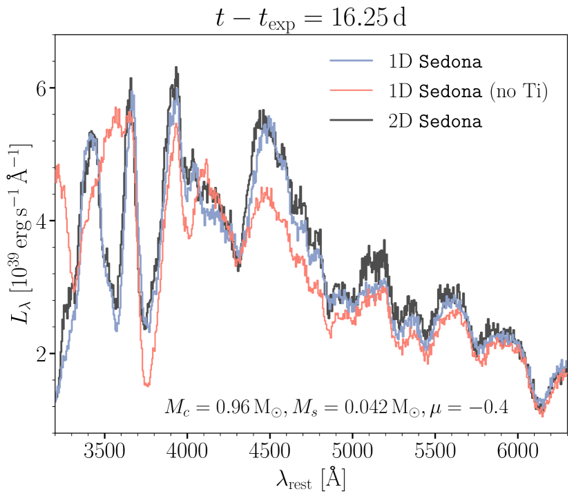
Figure 8: Comparison of the Sedona synthetic spectra at maximum luminosity indicates that Ti dominates the 4200 Å features in a double-detonation model. Two 1D Sedona models (blue + salmon pink) are run using the density and chemical profile of a slice between the viewing angles $\mu=-0.467$ and $\mu=-0.333$ of the $M_{c}=0.96\,\mathrm{M_{\odot}}$ and $M_{s}=0.042\,\mathrm{M_{\odot}}$ model from Boos et al. (2021). While the synthetic spectrum in the original 2D Sedona model can be well reproduced in a 1D run (blue), the model with all the titanium isotopes removed (salmon pink) cannot reproduce the remarkable 4200 Å features and exhibits a peak at $\sim$4100 Å.

The extremely red UV-optical colors near maximum luminosity are also broadly consistent with the double-detonation scenario, since the heavy elements (e.g., Ti, V, Cr, and Fe) in the outer ejecta could effectively absorb the UV photons with wavelengths around 3000 Å. However, no existing models could accurately model the UVOT light curves, especially in the $u$-band ($\sim$3100–3900 Å in the observed frame, or $\sim$3000–3800 Å in the rest frame of the host galaxy), where the flux is dominated by the re-emission of Ti, V, and Cr, and non-LTE effects could be important.

While none of the models presented here provide a strong match to SN 2022joj at every phase, we draw the broad conclusion that the spectroscopic properties of SN 2022joj are qualitatively consistent with a sub-$M_{\mathrm{Ch}}$ WD ($\gtrsim$1.0 $\mathrm{M_{\odot}}$) double detonation viewed from the hemisphere opposite to the ignition point. Observers from such a viewing angle would observe strong absorption features in the blue portion of the spectrum dominated by Ti as well as relatively shallow and slowly-expanding Si lines in the red portion. We emphasize that none of the models considered here was specifically developed and tuned to explain SN 2022joj. Customized models specifically tuned for SN 2022joj may reproduce all the observed features simultaneously, and we suggest more 2D double detonation simulations be performed. Furthermore, additional improvements can be made via an improved handling of the radiative transfer (e.g., non-LTE effects; see Shen et al., 2021a).

4.2 The 7300 Å Region in Nebular-Phase Spectra

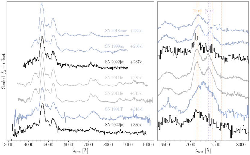
Figure 9: Nebular-phase spectra of SN 2022joj (black), three overluminous SNe Ia (blue), SN 1991T, SN 1999aa, and SN 2018cnw, and a normal SN Ia (gray), SN 2011fe. The right panel zooms in on the features around 7300 Å. The flux has been normalized to the [Fe III] features around 4700 Å. The orange dashed lines correspond to wavelengths of four [Fe II] lines (7155 Å, 7172 Å, 7453 Å, and 7638 Å), while the purple dotted lines correspond to the wavelengths of two [Ni II] lines (7378 Å, 7412 Å), both blueshifted by 1000 $\mathrm{km}\,\mathrm{s}^{-1}$. Spectra were downloaded from WiseREP (Yaron & Gal-Yam, 2012), with the following original data sources: SN 1991T and SN 1999aa – Silverman et al. (2012); SN 2011fe – Mazzali et al. (2015); SN 2018cnw – this work.

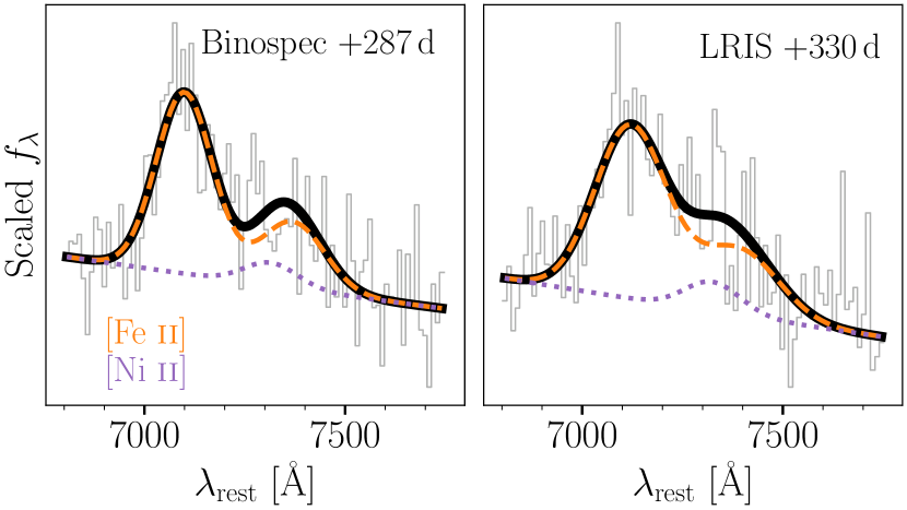
Figure 10: Fits to the 7300 Å region containing [Fe II] and [Ni II] features are consistent with a low Ni II abundance. The observed spectra are shown in gray. The colored lines correspond to the models of [Fe II] (orange) and [Ni II] (purple) features. For the model parameters we adopt the mean values of their posterior distributions. The black solid lines are the overall models.

In Figure 9 we compare the two nebular-phase spectra of SN 2022joj with the overluminous SNe Ia (SN 1991T, SN 1999aa, and SN 2018cnw) and the normal-luminosity SN 2011fe.

Compared to that of other SNe Ia, the nebular spectra of SN 2022joj show a relatively low flux ratio between the complex at $\sim$7300 Å (hereafter the 7300 Å features) dominated by [Fe II] and [Ni II] and the complex at $\sim$4700 Å dominated by [Fe III]. This suggests high ionization in the ejecta (Wilk et al., 2020). In addition to the smaller flux ratio, the profile of the 7300 Å features in SN 2022joj is also distinct from other SNe. Most of SNe Ia show a bimodal structure in their 7300 Å features (e.g., Graham et al., 2017; Maguire et al., 2018). The bluer peak is dominated by [Fe II] $\lambda\lambda$7155, 7172, while [Ni II] $\lambda\lambda$7378, 7412 usually have non-negligible contributions to the redder peak (see Figure 9). In some peculiar SNe Ia (mostly subluminous ones), the detection of [Ca II] $\lambda\lambda$7291, 7324 has also been reported (e.g. Jacobson-Galán et al., 2020; Siebert et al., 2020). The bimodal morphology is prominent in the spectra of SN 1999aa and SN 2011fe. SN 1999T is well-known for its broader emission lines in the nebular phase, so the composition of the 7300 Å features is ambiguous. In the spectra of SN 2022joj and SN 2018cnw, however, the redder peak is absent and the 7300 Å features show an asymmetric single peak, which seems to indicate a low abundance of Ni in the ejecta.

To investigate the relative contributions of [Fe II] and [Ni II] to the 7300 Å features in SN 2022joj, we model this region with multiple Gaussian emission profiles using the same technique as in Section 3.3. We include four [Fe II] lines (7155, 7172, 7388, 7453 Å) and two [Ni II] lines (7378, 7412 Å) in the fit. For each species, the relative flux ratios of lines are fixed, whose values are adopted from Jerkstrand et al. (2015). For [Fe II], we set $L_{7155}:L_{7172}:L_{7388}:L_{7453}=1:0.24:0.19:0.31$, and for [Ni II], we set $L_{7378}:L_{7412}=1:0.31$. These line ratios are calculated assuming LTE, but the departure from LTE should not be significant under the typical conditions in the ejecta (Jerkstrand et al., 2015). We allow the amplitudes $A$ of these Gaussian profiles to be either positive or negative. The velocity dispersions $\sigma_{v}$ in different lines of each species are set to be the same. For both $A$ and $\log\sigma_{v}$, we adopt flat priors, and only allow $\sigma_{v}$ to vary between 1000 and 6000 $\mathrm{km}\,\mathrm{s}^{-1}$. In addition, we adopt wide Gaussian priors for the radial velocities $v$ of [Fe II] and [Ni II], both centered at $-1000$ $\mathrm{km}\,\mathrm{s}^{-1}$ with a standard deviation of $2000$ $\mathrm{km}\,\mathrm{s}^{-1}$. The fitted models are shown in Figure 10, where colored curves correspond to the [Fe II] and [Ni II] emission adopting the mean values of the posterior distributions of model parameters sampled with MCMC. The fitted parameters are listed in Table 6. In both spectra, the flux of [Ni II] is consistent with 0 (${L_{[\mathrm{Ni}\,\textsc{ii}]\,\lambda 7378}}/{L_{[\mathrm{Fe}\,\textsc{ii}]\,\lambda 7155}}=0.13\pm 0.14$ at $+287$ days and $0.18\pm 0.16$ at $+330$ days; the flux ratios of lines are estimated with the ratios of their $p$EWs, and the uncertainties are the robust standard deviations estimated with the median absolute deviation of the drawn sample). We also find that the [Ni II] velocities cannot be constrained by the data, whose uncertainties estimated in both spectra are greater than the standard deviations of their Gaussian priors (2000 $\mathrm{km}\,\mathrm{s}^{-1}$), again disfavoring a solid [Ni II] detection. The 7300 Å features can be well fit with [Fe II] emission only. In addition, we have tested fitting this complex with [Ca II] in addition to [Fe II] and [Ni II], but find no evidence for [Ca II].

The relative abundance of Ni and Fe, which probes the mass of the progenitor WD, can be estimated via the flux ratio of their emission lines. At $>$300 days after explosion ⁵⁶Fe is the dominant isotope of Fe following the decay of ⁵⁶Ni through the chain ⁵⁶Ni$\rightarrow^{56}$Co$\rightarrow^{56}$Fe. Consequently, the Fe abundance primarily depends on the yield of ⁵⁶Ni. The Ni abundance, however, is sensitive to both the progenitor mass and the explosion scenario. The stable Ni isotopes (⁵⁸Ni, ⁶⁰Ni, and ⁶²Ni) are more neutron-rich compared to the $\alpha$-species ⁵⁶Ni, and can only be formed in high-density regions with an enhanced electron-capture rate during the explosion (Nomoto, 1984; Khokhlov, 1991). Consequently, SNe Ia from sub-$M_{\mathrm{Ch}}$ WDs, with central densities that are lower than near-$M_{\mathrm{Ch}}$ WDs, are expected to show a lower abundance of stable Ni isotopes (Iwamoto et al., 1999; Seitenzahl et al., 2013; Shen et al., 2018a).

To estimate the relative abundance of Ni and Fe, we use the equation adopted in Jerkstrand et al. (2015) and Maguire et al. (2018),

$$\frac{L_{7378}}{L_{7155}}=4.9\frac{n_{\mathrm{Ni}\,\textsc{ii}}}{n_{\mathrm{Fe}\,\textsc{ii}}}\exp\left(\frac{0.28\,\mathrm{eV}}{k_{B}T}\right)\frac{dc_{\mathrm{Ni}\,\textsc{ii}}}{dc_{\mathrm{Fe}\,\textsc{ii}}},$$ (1)

where $L_{7378}/L_{7155}$ is the flux ratio of the [Ni II] $\lambda$7378 to [Fe II] $\lambda$7155 lines, $n_{\mathrm{Ni}\,\textsc{ii}}/n_{\mathrm{Fe}\,\textsc{ii}}$ is the number density ratio of Ni II and Fe II, and ${dc_{\mathrm{Ni}\,\textsc{ii}}}/{dc_{\mathrm{Fe}\,\textsc{ii}}}$ is the ratio of the departure coefficients from LTE for these two ions. Since both Ni II and Fe II are singly ionized species with similar ionization potentials, we assume that $n_{\mathrm{Ni}\,\textsc{ii}}/n_{\mathrm{Fe}\,\textsc{ii}}$ is a good approximation of the total Ni/Fe ratio. As illustrated in Maguire et al. (2018), this assumption proves to be valid by modeling nebular-phase spectra at similar phases (Fransson & Jerkstrand, 2015; Shingles et al., 2022), with the relative deviation from the ionization balance $\lesssim$20%. We handle the uncertainties due to the unknown temperature, ratio of departure coefficients, and ionization balance in a Monte Carlo way. We randomly generate $N=4000$ samples of the temperature (3000–8000 K), the ratio of departure coefficients (1.2–2.4), and the ionization balance factor (0.8–1.2) assuming uncorrelated uniform distributions. These intervals are again adopted from Maguire et al. (2018). Combining these quantities with the samples of line-profile parameters drawn with the MCMC, we obtain $N$ estimates of Ni/Fe, which are effectively drawn from its posterior distribution. We find that Ni/Fe is consistent with 0 and we obtain a 3$\sigma$ upper limit of $\mathrm{Ni/Fe}<0.03$. Such a low Ni abundance is more consistent with the yields of sub-$M_{\mathrm{Ch}}$ double-detonation scenarios (Shen et al., 2018a), much lower than the expected outcomes of near-$M_{\mathrm{Ch}}$, delayed-detonation models (Seitenzahl et al., 2013) or pure deflagration models (Iwamoto et al., 1999).

Alternatively, it is proposed in Blondin et al. (2022) that for high-luminosity SNe Ia, the absence of [Ni II] lines can be a result of high ionization of Ni in the inner ejecta, despite the fact that a significant amount of Ni exists. It is shown that the [Ni II] $\lambda\lambda$7378, 7412 lines can be strongly suppressed even in a high-luminosity, near-$M_{\mathrm{Ch}}$ delayed-detonation model, once the Ni II/Ni III ratio at the center of the ejecta is artificially reduced by a factor of 10. Nevertheless, it remains to be questioned whether a physical mechanism exists to boost the ionization in the inner ejecta, where the stable Ni dominates the radioactive ⁵⁶Ni and ⁵⁶Co, and the deposited energy per particle due to the radioactive decay is usually low. One possible scenario is inward mixing, which brings ⁵⁶Co into the innermost ejecta such that the ionization would significantly increase. However, in this case calcium would inevitably be mixed inward as well, and the resultant Ca II $\lambda\lambda$7291, 7324 lines would stand out and dominate the 7300 Å features (Blondin et al., 2022). Other physical mechanisms are thus required to reduce the Ni II/Ni III ratio at the center of a near-$M_{\mathrm{Ch}}$ explosion.

We also find that the [Fe II] lines are significantly blueshifted ($v_{\mathrm{[Fe\,\textsc{ii}]}}=-(2.46\pm 0.38)\times 10^{3}\mathrm{\,km\,s^{-1}}$ at $+287$ days and $-(1.56\pm 0.60)\times 10^{3}\mathrm{\,km\,s^{-1}}$ at $+330$ days). This is consistent with other SNe Ia showing low $v_{\mathrm{Si\,\textsc{ii}}}$ at maximum brightness (Maeda et al., 2010b; Maguire et al., 2018; Li et al., 2021), and also in qualitative agreement with the asymmetric sub-$M_{\mathrm{Ch}}$ double-detonation scenario. Specifically, along a line of sight opposite to the shell detonation point, observers would see intermediate-mass elements (IMEs) with low expansion velocities, including Si II. In the meantime, the IGEs at the center of the ejecta would have a bulk velocity toward the observer (see Figure 1 and Figure 2 of Bulla et al., 2016; see also Fink et al., 2010).

Table 6: Fits to the late-time spectra around 7300 Å with [Fe II] and [Ni II] emission.

	[Fe II] $\lambda$7155			[Ni II] $\lambda$7378
Phase	$v$	$\sigma_{v}$	$p$EW	$v$	$\sigma_{v}$	$p$EW
(day)	($10^{3}$ $\mathrm{km}\,\mathrm{s}^{-1}$)	($10^{3}$ $\mathrm{km}\,\mathrm{s}^{-1}$)	(Å)	($10^{3}$ $\mathrm{km}\,\mathrm{s}^{-1}$)	($10^{3}$ $\mathrm{km}\,\mathrm{s}^{-1}$)	(Å)
$+286.8$	$-2.46\pm 0.38$	$2.98\pm 0.47$	$-129\pm 25$	$-2.89\pm 2.60$	$3.02\pm 1.45$	$-14\pm 19$
$+329.8$	$-1.56\pm 0.60$	$3.84\pm 0.80$	$-113\pm 28$	$-2.49\pm 2.44$	$3.11\pm 1.41$	$-13\pm 22$

4.3 Carbon Features at Maximum Luminosity

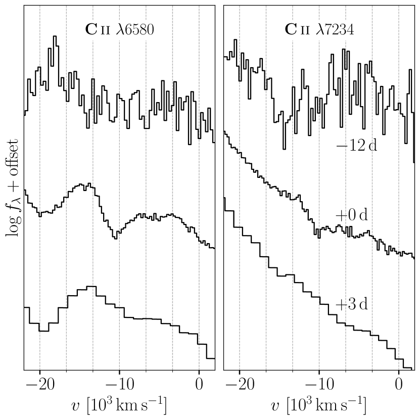
Figure 11: Prominent C II $\lambda\lambda$6580, 7234 absorption lines at maximum luminosity. No evident C II $\lambda$6580 lines are found in the earliest spectrum ($-12$ days; though there is one absorption feature that might be associated with C II $\lambda$7234 at $\sim$14,000 $\mathrm{km}\,\mathrm{s}^{-1}$) or the post-maximum spectrum ($+3$ days). All spectra are binned with a bin size of 5 Å, except for the low-resolution SEDM spectrum ($+3$ days). The dashed lines correspond to wavelengths of the C II lines assuming a range of velocities.

The spectrum at maximum luminosity exhibits strong C II $\lambda\lambda$6580, 7234 lines at a velocity of $\sim$10,000 $\mathrm{km}\,\mathrm{s}^{-1}$  (Figure 11). In the $-12$ days spectrum, we do not find strong evidence for the C II $\lambda$6580 line, though there is an absorption feature that might be associated with the C II $\lambda$7234 line at an expansion velocity of $\sim$$14,000$ $\mathrm{km}\,\mathrm{s}^{-1}$(see the right panel in Figure 11). The feature shows a velocity dispersion that is a factor of $\sim$3 greater than the unambiguous C II $\lambda$7234 line at maximum luminosity, and its nature remains vague. In this section we briefly discuss the possible origin of the carbon features.

In double detonations of sub-$M_{\mathrm{Ch}}$ WDs, the burning of carbon is expected to be efficient, with only a small fraction of carbon left unburnt. In 1D double-detonation models from Polin et al. (2019), only a negligible ($\lesssim$$10^{-5}\,\mathrm{M_{\odot}}$) amount of carbon is unburnt in normal and overluminous SNe, which should not cause any noticeable spectroscopic features. Multidimensional simulations produce a greater amount ($\sim$$10^{-4}$–$10^{-3}$ $\mathrm{M_{\odot}}$) of leftover carbon (Fink et al., 2010; Boos et al., 2021), which is still roughly two orders of magnitude lower than the yields of IMEs. Nevertheless, most of the unburnt carbon will be concentrated on the surface of the C/O core, forming a sharp carbon-rich shell (see Figures 5–8 in Boos et al., 2021) with a high expansion velocity ($>$10,000 $\mathrm{km}\,\mathrm{s}^{-1}$). Both 1D and 2D double-detonation models have low carbon yields in the helium ashes, so the carbon features may be strengthened over time, as the photosphere moves inward to the carbon-rich regions. Nevertheless, with the current resolution in the RT simulations, the contribution of such a sharp shell is unlikely to be captured in the resultant synthetic spectra.

Another possible origin of unburnt carbon in a double-detonation SN is the stripped material from a degenerate companion. In the Dynamically Driven Double-Degenerate Double-Detonation (D⁶) model (Shen et al., 2018b), the primary C/O WD could detonate following the dynamical ignition of a helium shell from its WD companion (either a helium WD or a C/O WD with a substantial helium envelope) during the unstable mass transfer (Guillochon et al., 2010; Pakmor et al., 2013). In this case, a significant amount ($\sim$$10^{-3}\,\mathrm{M_{\odot}}$) of materials can be stripped from a C/O WD companion, following the explosion of a 1 $\mathrm{M_{\odot}}$ primary WD (Tanikawa et al., 2018; Boos et al. 2023, in prep.), although the amount of carbon would likely be significantly less if the companion still holds a substantial helium envelope (Tanikawa et al., 2019). The velocity of the stripped carbon is expected to be low (e.g., centered at $\sim$3000 $\mathrm{km}\,\mathrm{s}^{-1}$ in Tanikawa et al., 2018), though more studies will need to be done to test the robustness of this estimate.

Explosion mechanisms that would result in a greater amount of unburnt carbon in the ejecta include the pure deflagration (Nomoto et al., 1984) or pulsating delayed detonation (Hoeflich et al., 1995; Dessart et al., 2014) of a near-$M_{\mathrm{Ch}}$ WD, and the violent merger of binary WDs (Raskin et al., 2014). None of these models reproduce the unusual red color in the early light curves or the peculiar spectroscopic features of SN 2022joj as well as the helium-shell double-detonation scenario does.

We conclude that while it remains to be questioned if double detonations could really produce strong carbon features, the detection of C II $\lambda\lambda$6580, 7234 lines in SN 2022joj does not necessarily invalidate our hypothesis of its double-detonation origin.

5 Conclusions

We have presented observations of SN 2022joj, a peculiar SN Ia. SN 2022joj has an unusual color evolution, with a remarkably red $g_{\mathrm{ZTF}}-r_{\mathrm{ZTF}}$ color at early times due to continuous absorption in the blue portion of its SED. Absorption features observed around maximum light simultaneously suggest high (a blue continuum and shallow Si II lines similar to those of overluminous, 99aa-/91T-like SNe) and low (the tentative Ti II features resembling those of subluminous, 91bg-like SNe) photospheric temperatures. The nebular-phase spectra of SN 2022joj suggest a high ionization and low Ni abundance in the ejecta, consistent with a sub-$M_{\mathrm{Ch}}$ explosion.

The early red colors are most likely due to a layer of IGEs in the outermost ejecta as products of a helium-shell detonation, in the sub-$M_{\mathrm{Ch}}$ double-detonation scenario. If the asymmetric ejecta are observed from the hemisphere opposite to the helium ignition point, we find that the resultant synthetic spectra could qualitatively reproduce some of the observed properties, including (i) significant line-blanketing of flux due to IGEs at early phases; (ii) strong absorption features around 4200 Å as well as relatively weak Si II features near maximum brightness, and (iii) blueshifted [Fe II] $\lambda$7155 accompanied with a relatively low expansion velocity of Si II at peak. Current double-detonation models cannot reproduce the strong C II lines in SN 2022joj at its maximum luminosity, but the double-detonation hypothesis is not necessarily disfavored and an improved RT treatment will be needed in modeling the observational effects of unburnt carbon. No existing double-detonation model can fully explain all the observational properties of SN 2022joj. As a result, it is possible that some alternative model is superior, though we find that the early red colors are difficult to explain with alternative explosion scenarios. Further refinement of multidimensional models covering a finer grid of progenitor properties may answer the question if the peculiar SN 2022joj is really triggered by a double detonation.

We thank the anonymous referee for a thoughtful report. We are grateful to Ping Chen, Avishay Gal-Yam, Anthony Piro, Anna Ho, and Jiaxuan Li for fruitful discussion, as well as Peter Blanchard and Jillian Rastinejad for the LRIS spectra they obtained. We acknowledge U.C. Berkeley undergraduate students Kate Bostow, Cooper Jacobus, Gabrielle Stewart, Edgar Vidal, Victoria Brendel, Asia deGraw, Conner Jennings, and Michael May for the Lick/Nickel photometry. K.J.S. was in part supported by NASA/ESA Hubble Space Telescope programs #15871 and #15918. S.J.B. and D.M.T. acknowledge support from NASA grant HST-AR-16156. L.H. is funded by the Irish Research Council under grant GOIPG/2020/1387. K.M. is funded by the EU H2020 ERC grant 758638. S.S. acknowledges support from the G.R.E.A.T. research environment, funded by Vetenskapsrådet, the Swedish Research Council, project 2016-06012. G.D. is supported by the H2020 European Research Council grant 758638. C.D.K. is partly supported by a CIERA postdoctoral fellowship. A.V.F.’s supernova group at U.C. Berkeley received generous financial assistance from the Christopher R. Redlich Fund, Briggs and Kathleen Wood (T.G.B. is a Wood Specialist in Astronomy), Alan Eustace (W.Z. is a Eustace Specialist in Astronomy), and numerous other donors.

We appreciate the excellent assistance of the staffs at the observatories where data were obtained. This work is based on observations obtained with the Samuel Oschin Telescope 48-inch and the 60-inch Telescope at the Palomar Observatory as part of the Zwicky Transient Facility project. ZTF is supported by the NSF under grant AST-2034437 and a collaboration including Caltech, IPAC, the Weizmann Institute of Science, the Oskar Klein Center at Stockholm University, the University of Maryland, Deutsches Elektronen-Synchrotron and Humboldt University, the TANGO Consortium of Taiwan, the University of Wisconsin at Milwaukee, Trinity College Dublin, Lawrence Livermore National Laboratories, IN2P3, University of Warwick, Ruhr University Bochum and Northwestern University. Operations are conducted by COO, IPAC, and UW. The SED Machine is based upon work supported by the NSF under grant 1106171. The ZTF forced-photometry service was funded under the Heising-Simons Foundation grant #12540303 (PI: Graham). The Gordon and Betty Moore Foundation, through both the Data-Driven Investigator Program and a dedicated grant, provided critical funding for SkyPortal.

A major upgrade of the Kast spectrograph on the Shane 3 m telescope at Lick Observatory, led by Brad Holden, was made possible through generous gifts from the Heising-Simons Foundation, William and Marina Kast, and the University of California Observatories. KAIT and its ongoing operation were made possible by donations from Sun Microsystems, Inc., the Hewlett-Packard Company, AutoScope Corporation, Lick Observatory, the U.S. NSF, the University of California, the Sylvia & Jim Katzman Foundation, and the TABASGO Foundation. Research at Lick Observatory is partially supported by a generous gift from Google.

This work is also based in part on observations made with the Nordic Optical Telescope, owned in collaboration by the University of Turku and Aarhus University, and operated jointly by Aarhus University, the University of Turku, and the University of Oslo (respectively representing Denmark, Finland, and Norway), the University of Iceland, and Stockholm University at the Observatorio del Roque de los Muchachos, La Palma, Spain, of the Instituto de Astrofisica de Canarias. The W. M. Keck Observatory is operated as a scientific partnership among the California Institute of Technology, the University of California, and NASA; the observatory was made possible by the generous financial support of the W. M. Keck Foundation. Observations reported here were obtained at the MMT Observatory, a joint facility of the Smithsonian Institution and the University of Arizona. W. M. Keck Observatory and MMT Observatory access was supported by Northwestern University and the Center for Interdisciplinary Exploration and Research in Astrophysics (CIERA).

This work has made use of data from the Asteroid Terrestrial-impact Last Alert System (ATLAS) project, which is primarily funded to search for near-Earth objects (NEOs) through NASA grants NN12AR55G, 80NSSC18K0284, and 80NSSC18K1575; byproducts of the NEO search include images and catalogs from the survey area. This work was partially funded by Kepler/K2 grant J1944/80NSSC19K0112 and HST GO-15889, and STFC grants ST/T000198/1 and ST/S006109/1. The ATLAS science products have been made possible through the contributions of the University of Hawaii Institute for Astronomy, the Queen’s University Belfast, the Space Telescope Science Institute, the South African Astronomical Observatory, and The Millennium Institute of Astrophysics (MAS), Chile.

PO:1.2m (ZTF), Swift (UVOT), KAIT, Nickel, Liverpool:2m (IO:O), PO:1.5m (SEDM), FTN (FLOYDS), FTS (FLOYDS), NOT (ALFOSC), Liverpool:2m (SPRAT), Keck:I (LRIS), MMT (Binospec), Hale (TSpec).

References

- Aihara et al. (2018) Aihara, H., Armstrong, R., Bickerton, S., et al. 2018, PASJ, 70, S8, doi: 10.1093/pasj/psx081
- Arbour et al. (1999) Arbour, R., Papenkova, M., Li, W. D., Filippenko, A. V., & Armstrong, M. 1999, IAU Circ., 7156, 1
- Astropy Collaboration et al. (2013) Astropy Collaboration, Robitaille, T. P., Tollerud, E. J., et al. 2013, A&A, 558, A33, doi: 10.1051/0004-6361/201322068
- Astropy Collaboration et al. (2018) Astropy Collaboration, Price-Whelan, A. M., Sipőcz, B. M., et al. 2018, AJ, 156, 123, doi: 10.3847/1538-3881/aabc4f
- Barbary et al. (2023) Barbary, K., Bailey, S., Barentsen, G., et al. 2023, SNCosmo, v2.10.0, Zenodo, doi: 10.5281/zenodo.7876632
- Bellm et al. (2019a) Bellm, E. C., Kulkarni, S. R., Graham, M. J., et al. 2019a, PASP, 131, 018002, doi: 10.1088/1538-3873/aaecbe
- Bellm et al. (2019b) Bellm, E. C., Kulkarni, S. R., Barlow, T., et al. 2019b, PASP, 131, 068003, doi: 10.1088/1538-3873/ab0c2a
- Blagorodnova et al. (2018) Blagorodnova, N., Neill, J. D., Walters, R., et al. 2018, PASP, 130, 035003, doi: 10.1088/1538-3873/aaa53f
- Blondin et al. (2022) Blondin, S., Bravo, E., Timmes, F. X., Dessart, L., & Hillier, D. J. 2022, A&A, 660, A96, doi: 10.1051/0004-6361/202142323
- Blondin & Tonry (2007) Blondin, S., & Tonry, J. L. 2007, ApJ, 666, 1024, doi: 10.1086/520494
- Boos et al. (2021) Boos, S. J., Townsley, D. M., Shen, K. J., Caldwell, S., & Miles, B. J. 2021, ApJ, 919, 126, doi: 10.3847/1538-4357/ac07a2
- Branch et al. (2004) Branch, D., Thomas, R. C., Baron, E., et al. 2004, ApJ, 606, 413, doi: 10.1086/382950
- Branch et al. (2006) Branch, D., Dang, L. C., Hall, N., et al. 2006, PASP, 118, 560, doi: 10.1086/502778
- Brown et al. (2018) Brown, P. J., Perry, J. M., Beeny, B. A., Milne, P. A., & Wang, X. 2018, ApJ, 867, 56, doi: 10.3847/1538-4357/aae1ad
- Brown et al. (2014) Brown, P. J., Kuin, P., Scalzo, R., et al. 2014, ApJ, 787, 29, doi: 10.1088/0004-637X/787/1/29
- Brown et al. (2013) Brown, T. M., Baliber, N., Bianco, F. B., et al. 2013, PASP, 125, 1031, doi: 10.1086/673168
- Bulla et al. (2016) Bulla, M., Sim, S. A., Kromer, M., et al. 2016, MNRAS, 462, 1039, doi: 10.1093/mnras/stw1733
- Bulla et al. (2020) Bulla, M., Miller, A. A., Yao, Y., et al. 2020, ApJ, 902, 48, doi: 10.3847/1538-4357/abb13c
- Burrow et al. (2020) Burrow, A., Baron, E., Ashall, C., et al. 2020, ApJ, 901, 154, doi: 10.3847/1538-4357/abafa2
- Byler et al. (2017) Byler, N., Dalcanton, J. J., Conroy, C., & Johnson, B. D. 2017, ApJ, 840, 44, doi: 10.3847/1538-4357/aa6c66
- Calzetti et al. (2000) Calzetti, D., Armus, L., Bohlin, R. C., et al. 2000, ApJ, 533, 682, doi: 10.1086/308692
- Carrick et al. (2015) Carrick, J., Turnbull, S. J., Lavaux, G., & Hudson, M. J. 2015, MNRAS, 450, 317, doi: 10.1093/mnras/stv547
- Cenko et al. (2006) Cenko, S. B., Fox, D. B., Moon, D.-S., et al. 2006, PASP, 118, 1396, doi: 10.1086/508366
- Chabrier (2003) Chabrier, G. 2003, PASP, 115, 763, doi: 10.1086/376392
- Chambers et al. (2016) Chambers, K. C., Magnier, E. A., Metcalfe, N., et al. 2016, arXiv e-prints, arXiv:1612.05560. https://arxiv.org/abs/1612.05560
- Childress et al. (2014) Childress, M. J., Filippenko, A. V., Ganeshalingam, M., & Schmidt, B. P. 2014, MNRAS, 437, 338, doi: 10.1093/mnras/stt1892
- Childress et al. (2013) Childress, M. J., Scalzo, R. A., Sim, S. A., et al. 2013, ApJ, 770, 29, doi: 10.1088/0004-637X/770/1/29
- Chu et al. (2022) Chu, M., Dahiwale, A., & Fremling, C. 2022, Transient Name Server Classification Report, 2022-1458, 1
- Conroy (2013) Conroy, C. 2013, ARA&A, 51, 393, doi: 10.1146/annurev-astro-082812-141017
- Conroy & Gunn (2010) Conroy, C., & Gunn, J. E. 2010, ApJ, 712, 833, doi: 10.1088/0004-637X/712/2/833
- Conroy et al. (2009) Conroy, C., Gunn, J. E., & White, M. 2009, ApJ, 699, 486, doi: 10.1088/0004-637X/699/1/486
- Coughlin et al. (2023) Coughlin, M. W., Bloom, J. S., Nir, G., et al. 2023, ApJS, 267, 31, doi: 10.3847/1538-4365/acdee1
- De et al. (2019) De, K., Kasliwal, M. M., Polin, A., et al. 2019, ApJ, 873, L18, doi: 10.3847/2041-8213/ab0aec
- De et al. (2020) De, K., Kasliwal, M. M., Tzanidakis, A., et al. 2020, ApJ, 905, 58, doi: 10.3847/1538-4357/abb45c
- de los Reyes et al. (2020) de los Reyes, M. A. C., Kirby, E. N., Seitenzahl, I. R., & Shen, K. J. 2020, ApJ, 891, 85, doi: 10.3847/1538-4357/ab736f
- Dekany et al. (2020) Dekany, R., Smith, R. M., Riddle, R., et al. 2020, PASP, 132, 038001, doi: 10.1088/1538-3873/ab4ca2
- Dessart et al. (2014) Dessart, L., Blondin, S., Hillier, D. J., & Khokhlov, A. 2014, MNRAS, 441, 532, doi: 10.1093/mnras/stu598
- Dey et al. (2019) Dey, A., Schlegel, D. J., Lang, D., et al. 2019, AJ, 157, 168, doi: 10.3847/1538-3881/ab089d
- Dong et al. (2022) Dong, Y., Valenti, S., Polin, A., et al. 2022, ApJ, 934, 102, doi: 10.3847/1538-4357/ac75eb
- Duev et al. (2019) Duev, D. A., Mahabal, A., Masci, F. J., et al. 2019, MNRAS, 489, 3582, doi: 10.1093/mnras/stz2357
- Eitner et al. (2022) Eitner, P., Bergemann, M., Ruiter, A. J., et al. 2022, arXiv e-prints, arXiv:2206.10258. https://arxiv.org/abs/2206.10258
- El-Badry et al. (2023) El-Badry, K., Shen, K. J., Chandra, V., et al. 2023, The Open Journal of Astrophysics, 6, 28, doi: 10.21105/astro.2306.03914
- Fabricant et al. (2019) Fabricant, D., Fata, R., Epps, H., et al. 2019, PASP, 131, 075004, doi: 10.1088/1538-3873/ab1d78
- Filippenko (1982) Filippenko, A. V. 1982, PASP, 94, 715, doi: 10.1086/131052
- Filippenko et al. (2001) Filippenko, A. V., Li, W. D., Treffers, R. R., & Modjaz, M. 2001, in Astronomical Society of the Pacific Conference Series, Vol. 246, IAU Colloq. 183: Small Telescope Astronomy on Global Scales, ed. B. Paczynski, W.-P. Chen, & C. Lemme, 121
- Filippenko et al. (1992a) Filippenko, A. V., Richmond, M. W., Matheson, T., et al. 1992a, ApJ, 384, L15, doi: 10.1086/186252
- Filippenko et al. (1992b) Filippenko, A. V., Richmond, M. W., Branch, D., et al. 1992b, AJ, 104, 1543, doi: 10.1086/116339
- Fink et al. (2010) Fink, M., Röpke, F. K., Hillebrandt, W., et al. 2010, A&A, 514, A53, doi: 10.1051/0004-6361/200913892
- Fitzpatrick (1999) Fitzpatrick, E. L. 1999, PASP, 111, 63, doi: 10.1086/316293
- Flörs et al. (2020) Flörs, A., Spyromilio, J., Taubenberger, S., et al. 2020, MNRAS, 491, 2902, doi: 10.1093/mnras/stz3013
- Foreman-Mackey et al. (2014) Foreman-Mackey, D., Sick, J., & Johnson, B. 2014, Python-Fsps: Python Bindings To Fsps (V0.1.1), v0.1.1, Zenodo, doi: 10.5281/zenodo.12157
- Fransson & Jerkstrand (2015) Fransson, C., & Jerkstrand, A. 2015, ApJ, 814, L2, doi: 10.1088/2041-8205/814/1/L2
- Fremling (2022) Fremling, C. 2022, Transient Name Server Discovery Report, 2022-1220, 1
- Galbany et al. (2019) Galbany, L., Ashall, C., Höflich, P., et al. 2019, A&A, 630, A76, doi: 10.1051/0004-6361/201935537
- Garavini et al. (2004) Garavini, G., Folatelli, G., Goobar, A., et al. 2004, AJ, 128, 387, doi: 10.1086/421747
- Gehrels et al. (2004) Gehrels, N., Chincarini, G., Giommi, P., et al. 2004, ApJ, 611, 1005, doi: 10.1086/422091
- Graham et al. (2019) Graham, M. J., Kulkarni, S. R., Bellm, E. C., et al. 2019, PASP, 131, 078001, doi: 10.1088/1538-3873/ab006c
- Graham et al. (2017) Graham, M. L., Kumar, S., Hosseinzadeh, G., et al. 2017, MNRAS, 472, 3437, doi: 10.1093/mnras/stx2224
- Guillochon et al. (2010) Guillochon, J., Dan, M., Ramirez-Ruiz, E., & Rosswog, S. 2010, ApJ, 709, L64, doi: 10.1088/2041-8205/709/1/L64
- Harris et al. (2020) Harris, C. R., Millman, K. J., van der Walt, S. J., et al. 2020, Nature, 585, 357, doi: 10.1038/s41586-020-2649-2
- HEASARC (2014) HEASARC. 2014, HEAsoft: Unified Release of FTOOLS and XANADU, Astrophysics Source Code Library, record ascl:1408.004. http://ascl.net/1408.004
- Hoeflich et al. (1995) Hoeflich, P., Khokhlov, A. M., & Wheeler, J. C. 1995, ApJ, 444, 831, doi: 10.1086/175656
- Howell et al. (2006) Howell, D. A., Sullivan, M., Nugent, P. E., et al. 2006, Nature, 443, 308, doi: 10.1038/nature05103
- Hunter (2007) Hunter, J. D. 2007, Computing in Science and Engineering, 9, 90, doi: 10.1109/MCSE.2007.55
- Inserra et al. (2015) Inserra, C., Sim, S. A., Wyrzykowski, L., et al. 2015, ApJ, 799, L2, doi: 10.1088/2041-8205/799/1/L2
- Iwamoto et al. (1999) Iwamoto, K., Brachwitz, F., Nomoto, K., et al. 1999, ApJS, 125, 439, doi: 10.1086/313278
- Jacobson-Galán et al. (2020) Jacobson-Galán, W. V., Polin, A., Foley, R. J., et al. 2020, ApJ, 896, 165, doi: 10.3847/1538-4357/ab94b8
- Jerkstrand et al. (2015) Jerkstrand, A., Smartt, S. J., Sollerman, J., et al. 2015, MNRAS, 448, 2482, doi: 10.1093/mnras/stv087
- Jiang et al. (2017) Jiang, J.-a., Doi, M., Maeda, K., et al. 2017, Nature, 550, 80, doi: 10.1038/nature23908
- Johnson et al. (2021) Johnson, B. D., Leja, J., Conroy, C., & Speagle, J. S. 2021, ApJS, 254, 22, doi: 10.3847/1538-4365/abef67
- Kasen (2010) Kasen, D. 2010, ApJ, 708, 1025, doi: 10.1088/0004-637X/708/2/1025
- Kasen et al. (2006) Kasen, D., Thomas, R. C., & Nugent, P. 2006, ApJ, 651, 366, doi: 10.1086/506190
- Kasen et al. (2003) Kasen, D., Nugent, P., Wang, L., et al. 2003, ApJ, 593, 788, doi: 10.1086/376601
- Khokhlov (1991) Khokhlov, A. M. 1991, A&A, 245, L25
- Kirby et al. (2019) Kirby, E. N., Xie, J. L., Guo, R., et al. 2019, ApJ, 881, 45, doi: 10.3847/1538-4357/ab2c02
- Kromer et al. (2010) Kromer, M., Sim, S. A., Fink, M., et al. 2010, ApJ, 719, 1067, doi: 10.1088/0004-637X/719/2/1067
- Leibundgut et al. (1993) Leibundgut, B., Kirshner, R. P., Phillips, M. M., et al. 1993, AJ, 105, 301, doi: 10.1086/116427
- Li et al. (2021) Li, W., Wang, X., Bulla, M., et al. 2021, ApJ, 906, 99, doi: 10.3847/1538-4357/abc9b5
- Lira (1996) Lira, P. 1996, Master’s thesis, -
- Liu et al. (2023a) Liu, C., Miller, A. A., Polin, A., et al. 2023a, ApJ, 946, 83, doi: 10.3847/1538-4357/acbb5e
- Liu et al. (2023b) Liu, Z.-W., Röpke, F. K., & Han, Z. 2023b, Research in Astronomy and Astrophysics, 23, 082001, doi: 10.1088/1674-4527/acd89e
- Livne (1990) Livne, E. 1990, ApJ, 354, L53, doi: 10.1086/185721
- Livne & Arnett (1995) Livne, E., & Arnett, D. 1995, ApJ, 452, 62, doi: 10.1086/176279
- Maeda et al. (2010a) Maeda, K., Taubenberger, S., Sollerman, J., et al. 2010a, ApJ, 708, 1703, doi: 10.1088/0004-637X/708/2/1703
- Maeda et al. (2010b) Maeda, K., Benetti, S., Stritzinger, M., et al. 2010b, Nature, 466, 82, doi: 10.1038/nature09122
- Magee & Maguire (2020) Magee, M. R., & Maguire, K. 2020, A&A, 642, A189, doi: 10.1051/0004-6361/202037870
- Magee et al. (2021) Magee, M. R., Maguire, K., Kotak, R., & Sim, S. A. 2021, MNRAS, 502, 3533, doi: 10.1093/mnras/stab201
- Maguire et al. (2014) Maguire, K., Sullivan, M., Pan, Y. C., et al. 2014, MNRAS, 444, 3258, doi: 10.1093/mnras/stu1607
- Maguire et al. (2018) Maguire, K., Sim, S. A., Shingles, L., et al. 2018, MNRAS, 477, 3567, doi: 10.1093/mnras/sty820
- Mahabal et al. (2019) Mahabal, A., Rebbapragada, U., Walters, R., et al. 2019, PASP, 131, 038002, doi: 10.1088/1538-3873/aaf3fa
- Maoz et al. (2014) Maoz, D., Mannucci, F., & Nelemans, G. 2014, ARA&A, 52, 107, doi: 10.1146/annurev-astro-082812-141031
- Masci et al. (2023) Masci, F. J., Laher, R. R., Rusholme, B., et al. 2023, arXiv e-prints, arXiv:2305.16279, doi: 10.48550/arXiv.2305.16279
- Masci et al. (2019) —. 2019, PASP, 131, 018003, doi: 10.1088/1538-3873/aae8ac
- Matheson et al. (2008) Matheson, T., Kirshner, R. P., Challis, P., et al. 2008, AJ, 135, 1598, doi: 10.1088/0004-6256/135/4/1598
- Mazzali et al. (1997) Mazzali, P. A., Chugai, N., Turatto, M., et al. 1997, MNRAS, 284, 151, doi: 10.1093/mnras/284.1.151
- Mazzali et al. (2014) Mazzali, P. A., Sullivan, M., Hachinger, S., et al. 2014, MNRAS, 439, 1959, doi: 10.1093/mnras/stu077
- Mazzali et al. (2015) Mazzali, P. A., Sullivan, M., Filippenko, A. V., et al. 2015, MNRAS, 450, 2631, doi: 10.1093/mnras/stv761
- Miller et al. (2020) Miller, A. A., Yao, Y., Bulla, M., et al. 2020, ApJ, 902, 47, doi: 10.3847/1538-4357/abb13b
- Miller & Stone (1994) Miller, J., & Stone, R. 1994, The Kast Double Spectograph, Lick Observatory technical reports (University of California Observatories/Lick Observatory). https://books.google.com/books?id=QXk2AQAAIAAJ
- Motohara et al. (2006) Motohara, K., Maeda, K., Gerardy, C. L., et al. 2006, ApJ, 652, L101, doi: 10.1086/509919
- Newsome et al. (2022) Newsome, M., Li, W., Burke, J., et al. 2022, Transient Name Server Classification Report, 2022-1274, 1
- Ni et al. (2022) Ni, Y. Q., Moon, D.-S., Drout, M. R., et al. 2022, Nature Astronomy, 6, 568, doi: 10.1038/s41550-022-01603-4
- Ni et al. (2023) —. 2023, ApJ, 946, 7, doi: 10.3847/1538-4357/aca9be
- Noebauer et al. (2017) Noebauer, U. M., Kromer, M., Taubenberger, S., et al. 2017, MNRAS, 472, 2787, doi: 10.1093/mnras/stx2093
- Nomoto (1982a) Nomoto, K. 1982a, ApJ, 253, 798, doi: 10.1086/159682
- Nomoto (1982b) —. 1982b, ApJ, 257, 780, doi: 10.1086/160031
- Nomoto (1984) —. 1984, ApJ, 277, 791, doi: 10.1086/161749
- Nomoto et al. (1984) Nomoto, K., Thielemann, F. K., & Yokoi, K. 1984, ApJ, 286, 644, doi: 10.1086/162639
- Nugent et al. (2011) Nugent, P. E., Sullivan, M., Cenko, S. B., et al. 2011, Nature, 480, 344, doi: 10.1038/nature10644
- Oke & Gunn (1982) Oke, J. B., & Gunn, J. E. 1982, PASP, 94, 586, doi: 10.1086/131027
- Oke & Gunn (1983) —. 1983, ApJ, 266, 713, doi: 10.1086/160817
- Oke et al. (1995) Oke, J. B., Cohen, J. G., Carr, M., et al. 1995, PASP, 107, 375, doi: 10.1086/133562
- Padilla Gonzalez et al. (2023a) Padilla Gonzalez, E., Howell, D. A., Burke, J., et al. 2023a, ApJ, 953, 25, doi: 10.3847/1538-4357/acdd6a
- Padilla Gonzalez et al. (2023b) Padilla Gonzalez, E., Howell, D. A., Terreran, G., et al. 2023b, arXiv e-prints, arXiv:2308.06334, doi: 10.48550/arXiv.2308.06334
- Pakmor et al. (2013) Pakmor, R., Kromer, M., Taubenberger, S., & Springel, V. 2013, ApJ, 770, L8, doi: 10.1088/2041-8205/770/1/L8
- Patat et al. (2012) Patat, F., Höflich, P., Baade, D., et al. 2012, A&A, 545, A7, doi: 10.1051/0004-6361/201219146
- Patterson et al. (2019) Patterson, M. T., Bellm, E. C., Rusholme, B., et al. 2019, PASP, 131, 018001, doi: 10.1088/1538-3873/aae904
- Pereira et al. (2013) Pereira, R., Thomas, R. C., Aldering, G., et al. 2013, A&A, 554, A27, doi: 10.1051/0004-6361/201221008
- Phillips et al. (2006) Phillips, A. C., Miller, J., Cowley, D., & Wallace, V. 2006, in Society of Photo-Optical Instrumentation Engineers (SPIE) Conference Series, Vol. 6269, Society of Photo-Optical Instrumentation Engineers (SPIE) Conference Series, ed. I. S. McLean & M. Iye, 62691O, doi: 10.1117/12.672469
- Phillips et al. (1999) Phillips, M. M., Lira, P., Suntzeff, N. B., et al. 1999, AJ, 118, 1766, doi: 10.1086/301032
- Piascik et al. (2014) Piascik, A. S., Steele, I. A., Bates, S. D., et al. 2014, in Society of Photo-Optical Instrumentation Engineers (SPIE) Conference Series, Vol. 9147, Ground-based and Airborne Instrumentation for Astronomy V, ed. S. K. Ramsay, I. S. McLean, & H. Takami, 91478H, doi: 10.1117/12.2055117
- Piro & Morozova (2016) Piro, A. L., & Morozova, V. S. 2016, ApJ, 826, 96, doi: 10.3847/0004-637X/826/1/96
- Piro & Nakar (2013) Piro, A. L., & Nakar, E. 2013, ApJ, 769, 67, doi: 10.1088/0004-637X/769/1/67
- Polin et al. (2019) Polin, A., Nugent, P., & Kasen, D. 2019, ApJ, 873, 84, doi: 10.3847/1538-4357/aafb6a
- Prochaska et al. (2020) Prochaska, J. X., Hennawi, J. F., Westfall, K. B., et al. 2020, Journal of Open Source Software, 5, 2308, doi: 10.21105/joss.02308
- Prochaska et al. (2020) Prochaska, J. X., Hennawi, J., Cooke, R., et al. 2020, pypeit/PypeIt: Release 1.0.0, v1.0.0, Zenodo, doi: 10.5281/zenodo.3743493
- Raskin et al. (2014) Raskin, C., Kasen, D., Moll, R., Schwab, J., & Woosley, S. 2014, ApJ, 788, 75, doi: 10.1088/0004-637X/788/1/75
- Rigault et al. (2019) Rigault, M., Neill, J. D., Blagorodnova, N., et al. 2019, A&A, 627, A115, doi: 10.1051/0004-6361/201935344
- Roming et al. (2005) Roming, P. W. A., Kennedy, T. E., Mason, K. O., et al. 2005, Space Sci. Rev., 120, 95, doi: 10.1007/s11214-005-5095-4
- Ruiter et al. (2011) Ruiter, A. J., Belczynski, K., Sim, S. A., et al. 2011, MNRAS, 417, 408, doi: 10.1111/j.1365-2966.2011.19276.x
- Ruiter et al. (2014) Ruiter, A. J., Belczynski, K., Sim, S. A., Seitenzahl, I. R., & Kwiatkowski, D. 2014, MNRAS, 440, L101, doi: 10.1093/mnrasl/slu030
- Salvatier et al. (2016) Salvatier, J., Wiecki, T. V., & Fonnesbeck, C. 2016, PeerJ Computer Science, 2, e55, doi: 10.7717/peerj-cs.55
- Sanders et al. (2021) Sanders, J. L., Belokurov, V., & Man, K. T. F. 2021, MNRAS, 506, 4321, doi: 10.1093/mnras/stab1951
- Schlafly & Finkbeiner (2011) Schlafly, E. F., & Finkbeiner, D. P. 2011, ApJ, 737, 103, doi: 10.1088/0004-637X/737/2/103
- Schulze et al. (2018) Schulze, S., Krühler, T., Leloudas, G., et al. 2018, MNRAS, 473, 1258, doi: 10.1093/mnras/stx2352
- Schulze et al. (2021) Schulze, S., Yaron, O., Sollerman, J., et al. 2021, ApJS, 255, 29, doi: 10.3847/1538-4365/abff5e
- Seitenzahl et al. (2013) Seitenzahl, I. R., Ciaraldi-Schoolmann, F., Röpke, F. K., et al. 2013, MNRAS, 429, 1156, doi: 10.1093/mnras/sts402
- Shen et al. (2021a) Shen, K. J., Blondin, S., Kasen, D., et al. 2021a, ApJ, 909, L18, doi: 10.3847/2041-8213/abe69b
- Shen et al. (2021b) Shen, K. J., Boos, S. J., Townsley, D. M., & Kasen, D. 2021b, ApJ, 922, 68, doi: 10.3847/1538-4357/ac2304
- Shen et al. (2018a) Shen, K. J., Kasen, D., Miles, B. J., & Townsley, D. M. 2018a, ApJ, 854, 52, doi: 10.3847/1538-4357/aaa8de
- Shen et al. (2018b) Shen, K. J., Boubert, D., Gänsicke, B. T., et al. 2018b, ApJ, 865, 15, doi: 10.3847/1538-4357/aad55b
- Shingles et al. (2021) Shingles, L., Smith, K. W., Young, D. R., et al. 2021, Transient Name Server AstroNote, 7, 1
- Shingles et al. (2022) Shingles, L. J., Flörs, A., Sim, S. A., et al. 2022, MNRAS, 512, 6150, doi: 10.1093/mnras/stac902
- Siebert et al. (2020) Siebert, M. R., Dimitriadis, G., Polin, A., & Foley, R. J. 2020, ApJ, 900, L27, doi: 10.3847/2041-8213/abae6e
- Silverman et al. (2012) Silverman, J. M., Foley, R. J., Filippenko, A. V., et al. 2012, MNRAS, 425, 1789, doi: 10.1111/j.1365-2966.2012.21270.x
- Smith et al. (2020) Smith, K. W., Smartt, S. J., Young, D. R., et al. 2020, PASP, 132, 085002, doi: 10.1088/1538-3873/ab936e
- Speagle (2020) Speagle, J. S. 2020, MNRAS, 493, 3132, doi: 10.1093/mnras/staa278
- Steele et al. (2004) Steele, I. A., Smith, R. J., Rees, P. C., et al. 2004, in Society of Photo-Optical Instrumentation Engineers (SPIE) Conference Series, Vol. 5489, Ground-based Telescopes, ed. J. Oschmann, Jacobus M., 679–692, doi: 10.1117/12.551456
- Tanikawa et al. (2018) Tanikawa, A., Nomoto, K., & Nakasato, N. 2018, ApJ, 868, 90, doi: 10.3847/1538-4357/aae9ee
- Tanikawa et al. (2019) Tanikawa, A., Nomoto, K., Nakasato, N., & Maeda, K. 2019, ApJ, 885, 103, doi: 10.3847/1538-4357/ab46b6
- Taubenberger (2017) Taubenberger, S. 2017, in Handbook of Supernovae, ed. A. W. Alsabti & P. Murdin (Springer), 317, doi: 10.1007/978-3-319-21846-5_37
- Taubenberger et al. (2011) Taubenberger, S., Benetti, S., Childress, M., et al. 2011, MNRAS, 412, 2735, doi: 10.1111/j.1365-2966.2010.18107.x
- Taubenberger et al. (2019) Taubenberger, S., Floers, A., Vogl, C., et al. 2019, MNRAS, 488, 5473, doi: 10.1093/mnras/stz1977
- Tody (1986) Tody, D. 1986, in Society of Photo-Optical Instrumentation Engineers (SPIE) Conference Series, Vol. 627, Instrumentation in astronomy VI, ed. D. L. Crawford, 733, doi: 10.1117/12.968154
- Tonry et al. (2018) Tonry, J. L., Denneau, L., Heinze, A. N., et al. 2018, PASP, 130, 064505, doi: 10.1088/1538-3873/aabadf
- Townsley et al. (2019) Townsley, D. M., Miles, B. J., Shen, K. J., & Kasen, D. 2019, ApJ, 878, L38, doi: 10.3847/2041-8213/ab27cd
- van der Walt et al. (2019) van der Walt, S., Crellin-Quick, A., & Bloom, J. 2019, The Journal of Open Source Software, 4, 1247, doi: 10.21105/joss.01247
- Wang & Wheeler (2008) Wang, L., & Wheeler, J. C. 2008, ARA&A, 46, 433, doi: 10.1146/annurev.astro.46.060407.145139
- Wang et al. (2003) Wang, L., Baade, D., Höflich, P., et al. 2003, ApJ, 591, 1110, doi: 10.1086/375444
- Wilk et al. (2020) Wilk, K. D., Hillier, D. J., & Dessart, L. 2020, MNRAS, 494, 2221, doi: 10.1093/mnras/staa640
- Woosley et al. (1986) Woosley, S. E., Taam, R. E., & Weaver, T. A. 1986, ApJ, 301, 601, doi: 10.1086/163926
- Woosley & Weaver (1994) Woosley, S. E., & Weaver, T. A. 1994, ApJ, 423, 371, doi: 10.1086/173813
- Yao et al. (2019) Yao, Y., Miller, A. A., Kulkarni, S. R., et al. 2019, ApJ, 886, 152, doi: 10.3847/1538-4357/ab4cf5
- Yaron & Gal-Yam (2012) Yaron, O., & Gal-Yam, A. 2012, PASP, 124, 668, doi: 10.1086/666656
- Zackay et al. (2016) Zackay, B., Ofek, E. O., & Gal-Yam, A. 2016, ApJ, 830, 27, doi: 10.3847/0004-637X/830/1/27
- Zheng et al. (2018) Zheng, W., Kelly, P. L., & Filippenko, A. V. 2018, ApJ, 858, 104, doi: 10.3847/1538-4357/aabaeb