Towards Packaging Unit Detection for Automated Palletizing Tasks

Abstract

For various automated palletizing tasks, the detection of packaging units is a crucial step preceding the actual handling of the packaging units by an industrial robot. We propose an approach to this challenging problem that is fully trained on synthetically generated data and can be robustly applied to arbitrary real world packaging units without further training or setup effort. The proposed approach is able to handle sparse and low quality sensor data, can exploit prior knowledge if available and generalizes well to a wide range of products and application scenarios. To demonstrate the practical use of our approach, we conduct an extensive evaluation on real-world data with a wide range of different retail products. Further, we integrated our approach in a lab demonstrator and a commercial solution will be marketed through an industrial partner.

I Introduction

The task of handling packaging units appears in all kinds of logistics use cases. Most notable here are the distribution centers in the supply chain of retailers, supermarkets, online shops or of general postal services; practically everywhere where orders with different products have to be put together or packages need to be sorted so that they can reach their destination. Other familiar everyday applications include filling supermarket shelves or accepting empties (Fig. 1), to name a few. Due to the high potential for automation in the handling of packaging units, Fraunhofer IPA has been working on this topic for several years now. It has become apparent that with a large and constantly changing product range, there are two main challenges. The first one is directly the physical manipulation of packaging units. They are usually close together and some of them, such as beverage or fruit crates, are open at the top and therefore cannot be picked with a suction or clamping gripper. As a solution to this problem, a so called roll-on-gripper [1] was developed and is now commercially available via Premium Robotics GmbH.

The other major challenge and subject of this work is the detection (identification and 3D pose estimation) of the packing units. Normally, only RGBD sensor data and, in some use cases, the dimensions of the packaging units from stock data are available for this purpose. Classical methods of computer vision typically fail due to sensor quality, especially transparent or reflective products are an issue here, and they are not able to generalize sufficiently well to arbitrary packaging units. Even state-of-the-art CNN-based object detectors are often limited to 2D bounding box regression and classification. They require large amounts of annotated data and training a network for each new product is practically not feasible. In addition to the accuracy of the required annotations, the sparse depth information caused by the physical principle of most depth sensors poses another problem.

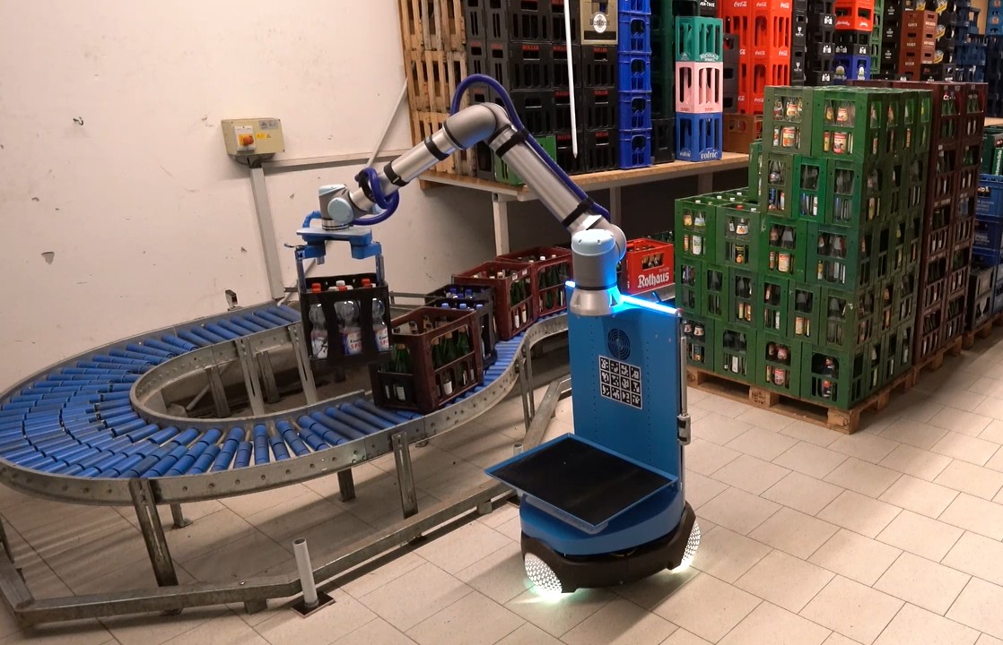
Figure 1: Beverage logistics with a mobile handling robot

Generic CNN-based state-of-the-art 3D object detectors [2] are mostly extensions of 2D single shot detectors, while some approaches are specialized for industrial applications [3] in which RGBD sensors are available, but none of them can be directly used for general packaging unit detection. In this paper we address these challenges and present an industrially applicable framework for the most relevant scenarios of packaging unit detection. We further distinguish between homogeneous pallet stacks, with only one kind of product and heterogeneous pallet stacks which contain several different packaging units or products. We refer to the dimension (long, short, height) of the packing units as box size and consider the following scenarios.

• Homogeneous pallet stacks with known box size: This is typically the case when orders of supermarkets etc. have to be fulfilled and heterogeneous pallet stacks have to be build in distribution centers. An additional issue in this case are intermediate layers (interlayers) which are layers of cardboard between the packaging units to stabilize the stack. They typically have to be detected and removed before the next layer can be handled.

• Heterogeneous pallet stacks and box size is not known: This is the case when packaging units have to be identified for delivery services, accepting empties etc.

• Heterogeneous pallet stacks with known box size: Searching for boxes on a pallet stack for restocking shelves in a supermarket or retail shop for instance.

The main contributions of this paper are as follows:

• An industrial grade framework/solution for the challenging task of packaging unit detection for palletizing tasks. The approach generalizes to arbitrary real world packaging units and objects of cuboid shape without any additional training.

• A valuable auxiliary prediction task for single-shot object detectors.

• A dynamically scaling loss function with fast convergence that can be applied to classification and regression tasks as well, while it can handle the influence of outliers and simultaneously large class imbalance.

• A general mechanism for estimating the prediction quality of neural networks in general and especially for single-shot object detectors.

• An extensive evaluation of our detection framework on a depalletizing task and its application to various beverage logistics scenarios (Fig. 1).

II Related Work

II-A Packaging Unit Detection

Publications on the challenging problem of general packaging unit detection are scarce. Most of them focus on depalletizing and are limited to special cases like cardboard parcel boxes [4, 5] or are based on model-driven bin picking [6]. The typical approach to this problem is based on classical Computer Vision (CV) for feature detection [7, 8] and solving a combinatorial optimization problem [7, 4]. Others build on even stronger simplifications such as RFID-Tags [9] or focus on hardware and the overall architecture [10]. Non of these approaches is able to generalize to arbitrary packing units in homogeneous and heterogeneous pallet stacks while being robust against sensor limitations and environmental conditions. Our proposed framework for packaging unit detection fulfills all this requirements. It generalizes to arbitrary packing units or objects of cuboid shape without the need of further training or manual setup and can perform the detection in less then 100 ms.

II-B Relevant Learning Techniques

Single-shot object detectors like SSD [11], YOLO [12, 13] or RetinaNet [14] are current state-of-the-art in terms of prediction quality and speed. They are typically fully conventional Convolutional Neural Networks that make local predictions for object classification and a bounding box regression, which are subsequently filtered in post-processing step called Non Maximum Suppression (NMS). Their training with basic loss functions such as the Binary Cross Entropy (BCE) and L2 loss face three main issues. The first issue is the imbalance of classes in the local classification ground truth. This can either be addressed by a sampling strategy known as Online Hard Example Mining (OHEM) [15] or more recently by loss functions like the Focal Loss (FL) [14], the Reduced Focal Loss (RFL) [16] or the Shrinkage Loss (SL) [17] which automatically weight down easy samples based on their absolute error.

The second issue are outliers resulting from low quality bounding box annotations done by humans. One approach to reduce their influence is a combination between L1 and L2 loss called the Huber Loss [18] or more popular its special case the Smooth L1 Loss [19]. The third issue also considers bounding box regression and arises from the large variance in object scale. Recent approaches like the Distance IoU Loss [20] solve this issue by utilizing scale independent metrics like the Intersection over Union (IoU). Other recent approaches [21, 22] perform quality estimates which are later used in the post-processing step to suppress bounding boxes with low quality. Two of these quality estimates are the center-ness score [21] and the IoU score [22], whereby the predicted IoU is an estimate derived from an other estimate, the bounding box prediction. In Section III we propose a unified loss function that addresses all these issues and a generalized quality estimate for arbitrary local predictions.

The last years have brought some improvements and specializations concerning the convolution operation and the architecture of CNNs, which we will use in Section IV. Separable Convolutions [23, 24] are used in Inverted Residual blocks or MBConv blocks [25] to heavily (90% or more) reduce parameter count without notable performance loss. Adding the spatial location on which the convolution kernel is applied on the feature map as additional features to convolution input [26] improves the performance for practically all tasks which require more spatial or contextual information. Sparse [27] and Partial Convolution [28] where proposed to handle sparse input directly in the network by propagating the sparsity signal through the network and considering it in the convolution operation. Furthermore, it has been shown [29] that object detectors trained on synthetically generated data can outperform ones trained on real images under the right circumstances and that Physically Based Rendering (PBR) [30] outperforms other methods of synthetic data generation. Also, adding additional sparsity to the input data is not necessarily a harmful undertaking. It can be used as valuable auxiliary task for learning representation for language [31] or vision [32] task and works as regularization like in the well known Dropout [33].

III General Contributions

This section introduces some novel concepts for generic single-shot detectors which we will later use in our proposed detection framework.

III-A Bounded Distance Transform

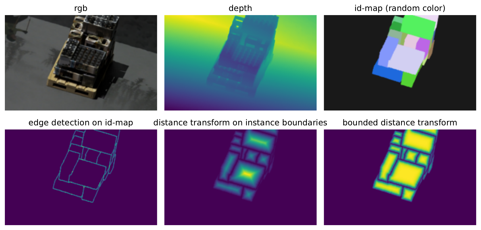
Figure 2: Bounded Distance Transform (rendered image data with orthographic camera)

We propose an auxiliary prediction task that can be used in the post-processing step (NMS) to efficiently separate instances and suppress uncertain predictions near the instance boundary. In the following, we call the ground truth for this task and its computation the Bounded Distance Transform (BDT). The steps for obtaining the BDT $d_{b}$ from id-maps or segmentation ground truth are visualized in Fig. 2. First we use Sobel filters for detecting the instance boundaries from the id-maps. Second we perform the Euclidean Distance Transform [34] on the edges representing the instance boundaries and set the background areas to zero. As third and last step we use the $\tanh$ to bring the values into the interval $[0,1]$ and keep them near $1$ on the inside of the instances.

$$d_{b}=\tanh{\frac{d}{s}}$$ (1)

Here, $d$ refers to the Euclidean Distance Transform and $s$ to a scaling factor which we choose based on the down-sampling ratio of our CNN-architecture to get suitable ground truth.

Predictions of the BDT can later in the post-processing be used for thresholding while the $\tanh$ prevents small instances from being ignored. It should also be possible to directly use a prediction of the BDT for instance segmentation. For this it would make sense to perform a morphological operation with suitable kernel size to compensate the too small instance masks resulting from thresholding. All the necessary operations for the BDT can be done using classical CV libraries like OpenCV [35] and to the best of our knowledge, this simple but efficient idea was not published before.

III-B Dynamically Scaled Shrinkage Loss

In this section we propose a loss function that dynamically scales the absolute error before passing it through its nonlinearity. Since we build on the idea of the well known Shrinkage Loss [17], we call our proposed loss function the Dynamically Scaled Shrinkage Loss (DSSL). The DSSL can be applied to classification and regression problems as well.

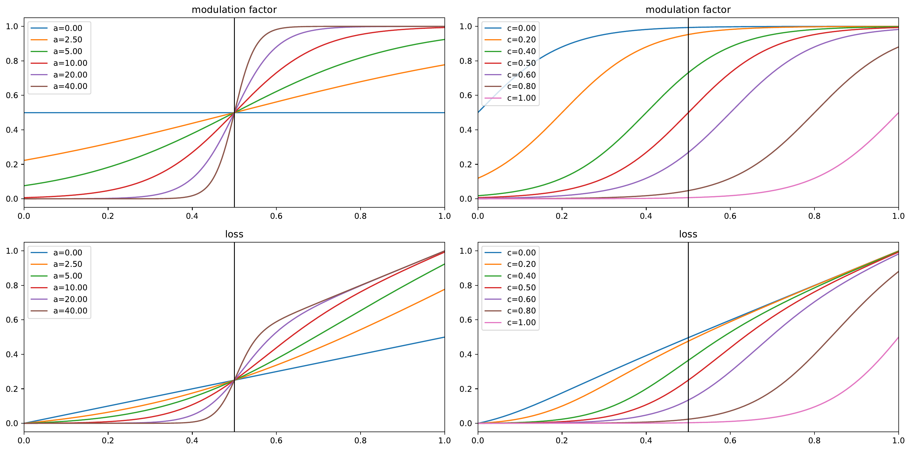
Figure 3: Influence of the parameters $a$ (left) and $c$ (right) on the modulation factor Eq. 5 (top) and the loss function Eq. 6 (bottom) depending on the absolute or respectively the normalized absolute error

In the following, we consider the local predictions on a feature map with shape $B\times H\times W\times K$, with $b$, $h$, $w$ and $k$ as the indices on this feature map. $B$ represents the batch size, $H$ and $W$ the spatial dimensions height and width and $K$ the number of considered channels, for instance, $K$ confidences for the classification of $K$ classes. The absolute error for one element can then be written as

$$l_{bhwk}=\left|y_{bhwk}-\hat{y}_{bhwk}\right|$$ (2)

where $y$ denotes the local ground truth and $\hat{y}$ the prediction of the network. Starting with the average absolute error within a batch $\bar{l}$

$$\bar{l}=\frac{1}{BHWK}\sum_{b=1}^{B}\sum_{h=1}^{H}\sum_{w=1}^{W}\sum_{k=1}^{K}l_{bhwk}$$ (3)

we can write a normalized form $n_{bhwk}$ of the absolute error

$$n_{bhwk}=\frac{l_{bhwk}}{2\mathrm{gs}\left(\bar{l}\right)+\epsilon}$$ (4)

Where $\mathrm{gs}(\cdot)$ stops the gradient propagation during training. $\epsilon$ is a small constant for numerical stability. Utilizing the modulation factor $f(l)$ with its parameters $a$ and $c$ from Shrinkage Loss

$$f(l)=\frac{1}{1+\exp{a(c-l)}}$$ (5)

we can formulate the following local loss function

$$L_{bhwk}=\frac{n_{bhwk}}{1+\exp{a(c-n_{bhwk})}}$$ (6)

which leads to our global loss function

$$L_{DSSL}=\frac{1}{BHW}\sum_{b=1}^{B}\sum_{h=1}^{H}\sum_{w=1}^{W}\sum_{k=1}^{K}L_{bhwk}$$ (7)

The proposed DSSL has some notable properties. The dynamic scaling of the absolute errors has the consequence that the loss function always operates around its inflection point at $0.5$. Replacing $n_{bhwk}$ by $l_{bhwk}$ in Eq. 6 disables the dynamic scaling behavior. Instead of the squared absolute error in the SL, we use the absolute respectively the normalized absolute error in the nominator of Eq. 6. This avoids a second nonlinearity, reduces the influence of outliers and makes things more interpretable. Fig. 3 shows the influence of the parameters $c$ and $a$ on the modulation factor and the loss function itself. Fig. 4 compares DSSL with other loss functions. It has the property of down-weighting the easy samples as it is done by the FL while at the same time reducing the influence of outliers as it is done by the Smooth L1 Loss. Smooth L1 and FL have also the drawback of nearly vanishing gradients for small regression errors. Due to the dynamic scaling we always get strong error signals and let the training dynamics do the rest while we reduce the learning rate during training. Another consequence of the normalization is that the loss value no longer decreases during training (Fig. 9). Therefore, the absolute error may be a better choice for monitoring the training progress. One may also consider to maintain a moving average of the mean absolute error, but in our experiments, we found that the statistic over batch and spatial dimensions are sufficient for fast and stable convergence. If we apply the DSSL with our default parameters ($a=20$ and $c=0.5$) to a classification task like the one shown in Figs. 14 and 15 (background, short, long), it rapidly fits the binary labels. For smoother values that look more like a probability distribution as produced by the FL, it would make sense to choose the parameters $a$ and $c$ more suitable, but for most classification tasks simply the $\mathrm{argmax}$ function is used. Also for bounding box regression it may be desired to get an error signal that is independent of the actual object scale, as with IoU Loss (Section II-B). This can be achieved by dividing the absolute error after Eq. 2 by the object scale. We provide our implementation of DSSL in TensorFlow.

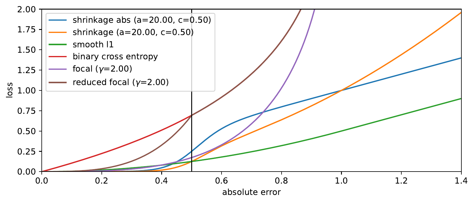
Figure 4: Comparison of various loss functions; we use ’shrinkage abs’ for the DSSL, where the mean absolute error is dynamically scaled to $0.5$

III-C Prediction of Certainty

In this section we propose a generalization of the quality estimate mentioned in Section II-B. The basic idea here is simple, let the network estimate its own prediction error. A direct prediction of the regression error as a quantitative measure may be difficult to handle in a post-processing (NMS) step, at least if a certain threshold has to be determined. Therefore, based on Eq. 2 and Eq. 3, we propose a unified quality measure Eq. 8 which is defined in the interval $[0,1]$ and where higher is better.

$$\text{certainty}_{bhwk}=\exp\left(\frac{l_{bhwk}}{\mathrm{gs}\left(\bar{l}\right)+\epsilon}\log\frac{1}{2}\right)$$ (8)

The plot in Fig. 5 shows a graph of the proposed certainty function, which is $0.5$ for the average error, $1$ for an error of $0$ and $0$ for an infinitely large error. As our intuition suggests and [22] have shown, the backpropagation of the gradient resulting from the actual prediction is not beneficial for the overall performance. Therefore we also stop the gradient propagation at this place. The training can be done via the DSSL proposed in Section III-B.

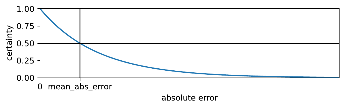
Figure 5: Certainty function as defined in Eq. 8

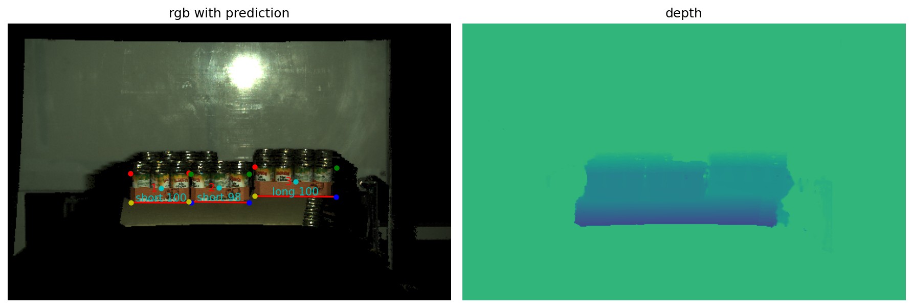
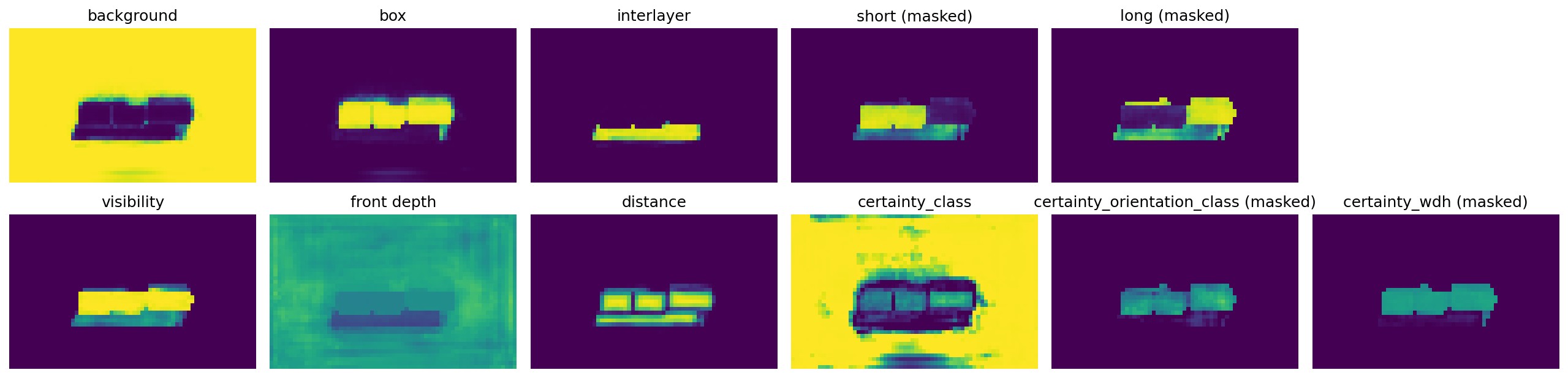
Figure 16: Prediction on orthographic projected real data

Our first experiments in Fig. 16 indeed show that the predicted certainty is low in areas with insufficient information or ambiguity due to partially hidden objects etc.

IV Packaging Unit Detection

IV-A Data Generation

Object detectors $\hat{f}(x)$ in general, approximate a function $y=f(x)$ based on a finite number of training samples $(X_{n},Y_{n})_{n=1}^{N}$, where $y$ denotes the abstract representation of the objects (category, position, orientation, …) and $x$ denotes the sensor data corresponding to the scene. Since human annotations on real 3D sensor data are laborious and often inaccurate, it is much easier and more flexible to model the inverse $f^{-1}(y)$ of this function using computer graphics and sample training data from this simulated distribution.

We utilize Blender to render photorealistic scenes of pallet stacks and get the corresponding ground truth (Fig. 7) without manual annotations. During this process of procedural data generation we randomize certain scene properties like camera view, lighting, background as well as the packaging pattern and the size and type of the packaging units themselves. We model certain specific types of packaging units like, boxes, bags, beverage crates and closed and open cartboard boxes (fruit and vegetables) etc., as well as their content in form of cans, bottles, packages (beverage cartons, cardboard packages, etc.) or random stuff. For the packaging units, their content, the background and additional disturbance geometry, we excessively randomize the geometry using tessellation, the texture and the material properties in form of the shader parameterization. To achieve robustness against the noise and sparsity resulting from sensor limitations we add several artifacts to the synthesized sensor data. We add Gaussian noise with random standard deviation to mimic sensor noise and Gaussian blur with random kernel size and standard deviation to mimic blur resulting from various intrinsic filtering techniques. In addition we add artificial sparsity as shown in Fig. 6. These binary masks are a combination of binary noise drawn from a Bernoulli distribution, dilated binary noise and random polygons and elliptic shapes that mimic large sharp and round sparse areas resulting from the physical measuring principle of the sensors.

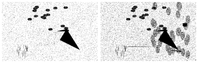
Figure 6: Random artificial sparsity for RGB image (left) and with additional sparsity on depth image (right)

In summary we get the simulated sensor data in form of RGB and depth images and the ground truth for packaging unit detection in form of size, position, orientation, keypoints (top-lef, top-right, bottom-right, bottom-left corner of the front and back side of the packaging unit) in image and 3D space, visibility values and id-maps for instance segmentation. The visibility is the percentage of a packaging unit instance that is not occluded by other instances. An estimate of the visibility may later be helpful to decide whether a packaging unit can be picked or not.

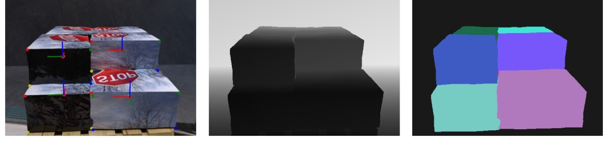
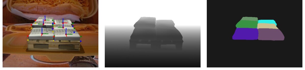
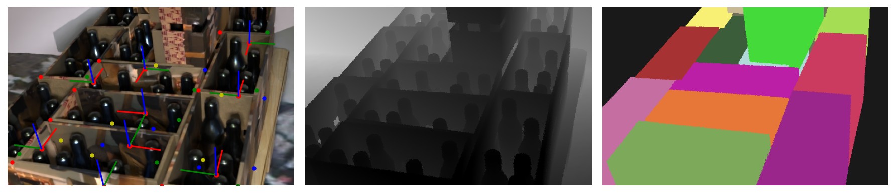
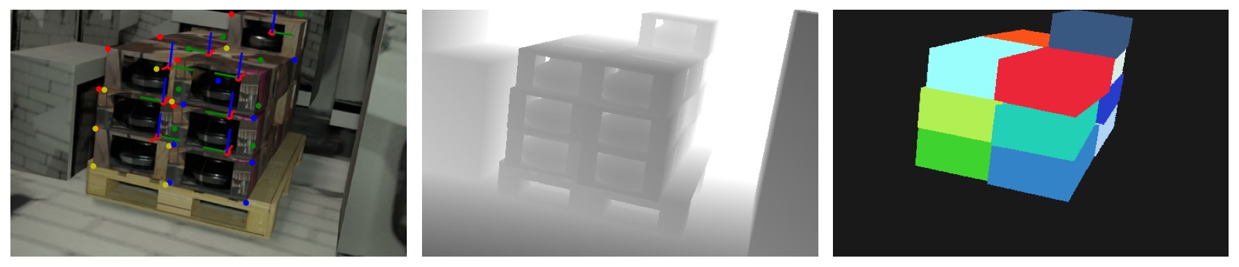
Figure 7: Synthetically generated data; RGB image with (left), depth image (middle) and segmentation ground truth / id-map (right), detection ground truth (box frame and keypoints) drawn in RGB image

IV-B Architecture

For the special case of packaging unit detection, we propose a suitable fully convolutional network architecture, shown in Fig. 8, that directly results from the prior work mentioned in Section II-B. We use two separate encoder based MBConv blocks combined with Partial Convolution to handle sparse input data and concatenate the features together. We then use 1x1 convolution and dilated convolution to change the number of features and aggregate more spatial information. After a second stage of MBConv blocks we concatenate the tiled box size to the feature map. We also add the spatial location of elements on the feature map as additional features [26] and end up with a third and fourth stage in two separate branches, one for the classification and one for the regression part. We use Rectified Linear Unit (ReLU) activation functions for the whole architecture except for final output activation which we choose appropriately to the prediction (softmax, sigmod or linear). The local predictions of the network contain a classification (background, box and interlayer), a second classification for the box orientation (short, long), a confidence for the prior (whether the detected instance fits to the prior / provided box size or not), visibility, relative key points in image space, keypoints in 3D, position and orientation (elements of a rotation matrix) in 3D, distance of the front face, box dimension (short, long, height), box dimension (width, depth, height), the BDT proposed in Section III-A and the certainty (Section III-C) for classification, orientation classification and box size regression.

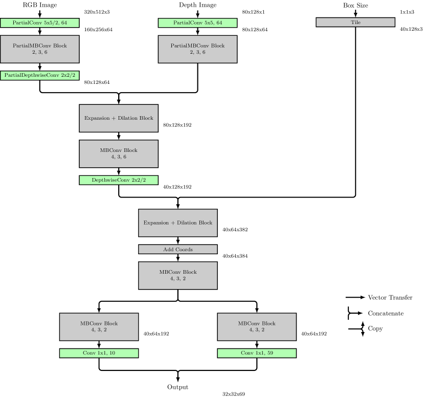
Figure 8: Architecture of the proposed network; notation for Conv: kernel_size/stride, features; notation for MBConv: repeats, kernel_size, expansion

IV-C Training

For all predictions, we use the DSSL proposed in Section III-B. To handle the symmetries of packaging units along the z-axis (bottom to top) for the prediction of the orientation, we calculate the loss values for all valid orientations and select the smallest value for backpropagation. Depending on the use case, we decide whether we use training data with homogeneous or heterogeneous pallet stacks and whether we can omit the rightmost branch in Fig. 8 providing the box size. It is clear, that the model will learn to make the best predictions for the case of homogeneous pallet stacks and known box size. For the more challenging use case with heterogeneous pallet stacks and unknown box size, the model has to learn to predict the box dimensions. It may also be easier to learn the box dimensions in form (width, depth, height) in camera view instead of (short, long, height), where rotation comes into play and the box prediction may totally fail due to a wrongly estimated depth dimension for instance. In the case of heterogeneous pallet stacks and known box size, the model will learn to distinguish the packaging units from others via the prior confidence and will also do a better job on estimating their position and orientation.

IV-D Prediction and Post-Processing

In this section we consider the post processing step for filtering the dense predictions from the CNN output. In addition to the direct pose regression for the instances, we also reconstruct their pose from the 3D keypoint regression. To select good candidates from the local predictions, we filter them based on classification, visibility, BDT and certainty. We group the remaining candidates based on their minimum box dimension and their Euclidean distance to each other before we select the candidate that is nearest to the spatial mean of each group. Finally, we sort the remaining predictions in the pallet coordinate system which is either known directly or a rough estimate is available. We sort them suitable for the application and based on their height, from top to bottom and from near to far.

V Application

V-1 Implementation

During our work, we trained different sensor specific models and one on orthographic projections which is independent of the intrinsic sensor parameters. Namely, we trained models for the Intel® RealSense D435 which is rather low-cost and for the Zivid One+ Large which provides sensor data with higher quality. We trained each model on roughly 120k generated training samples and used 2k for validation. The training itself was performed on one NVIDIA V100 GPU, with batch size 12 and Adam as optimizer. We started our training with an initial learning rate of $0.001$ and reduced it by half after 225k, 300k, 375k, 450k iterations respectively. Some plots from the training process are shown in Fig. 9.

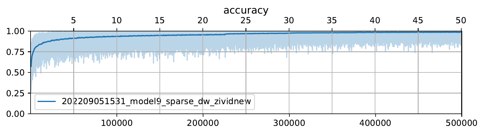
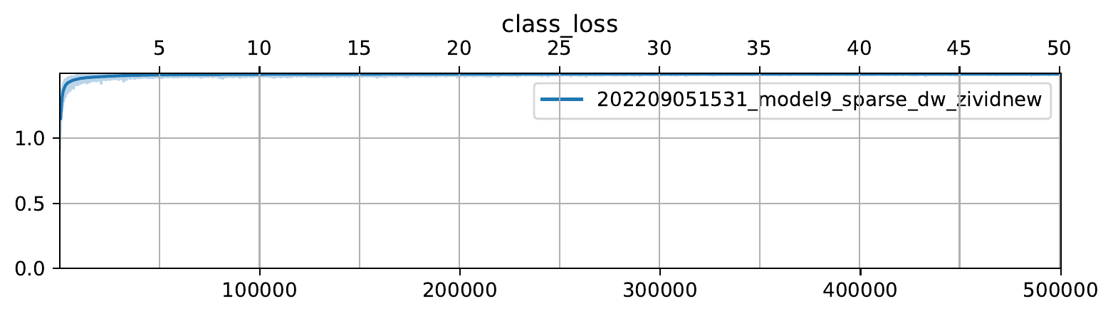
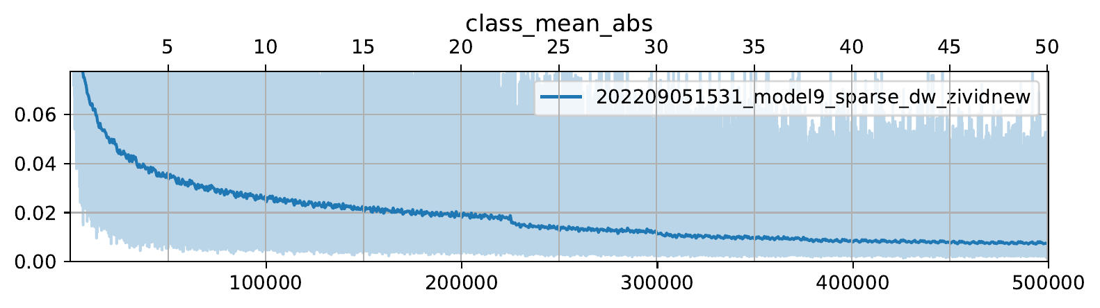
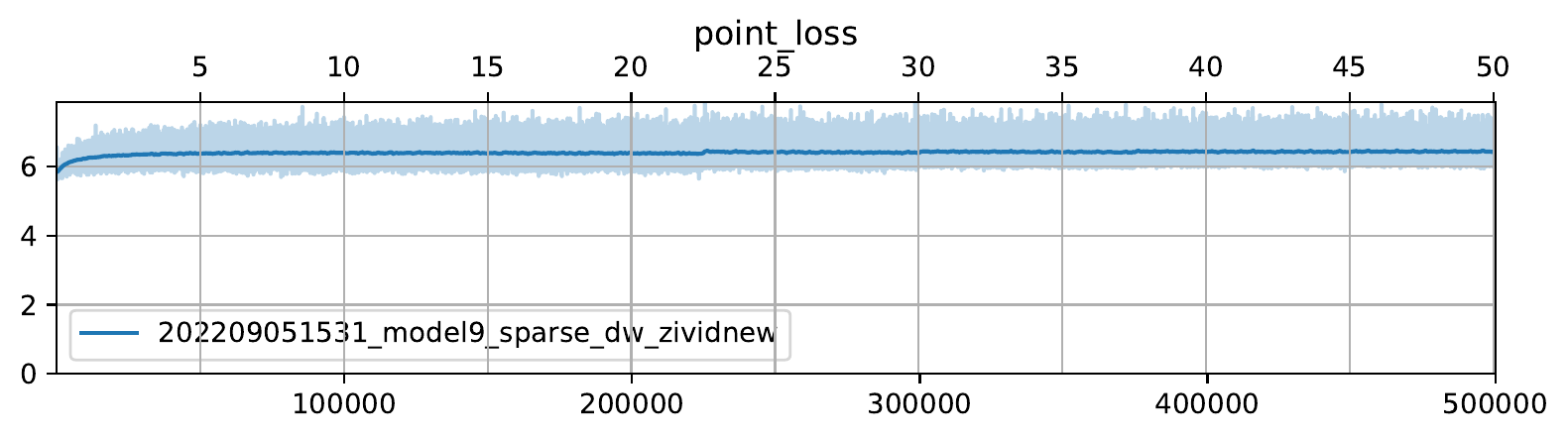
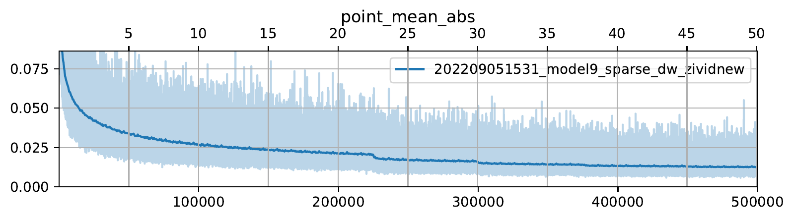
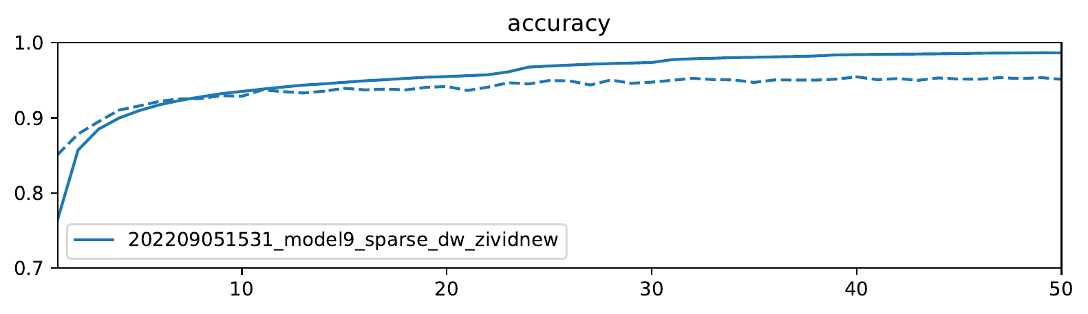
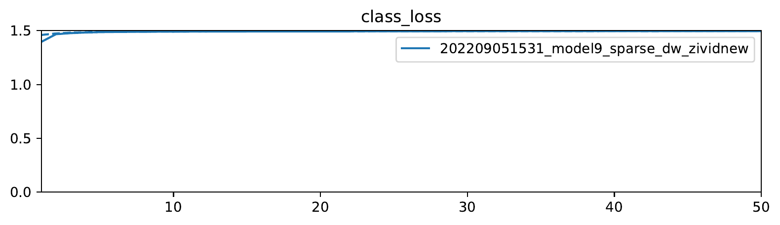
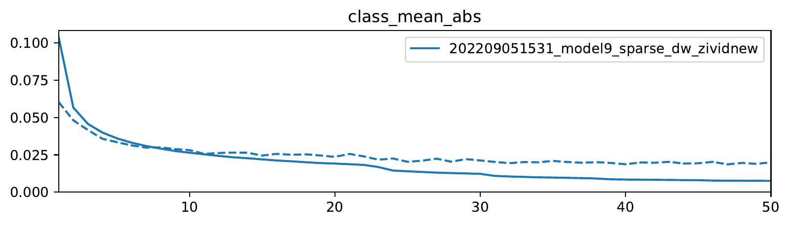
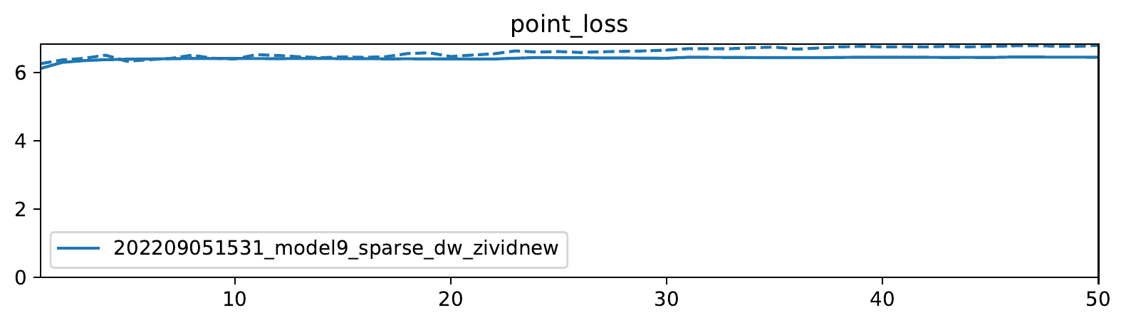
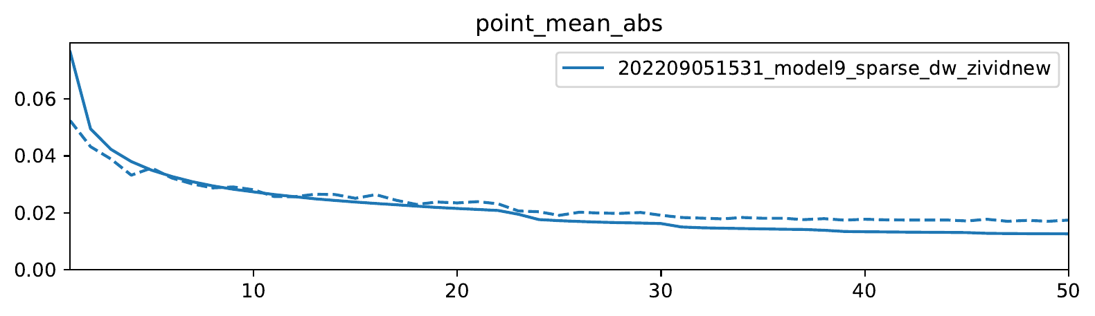
Figure 9: Training log (left) and history (right); iterations on the bottom, epochs on top; dashed lines represent validation

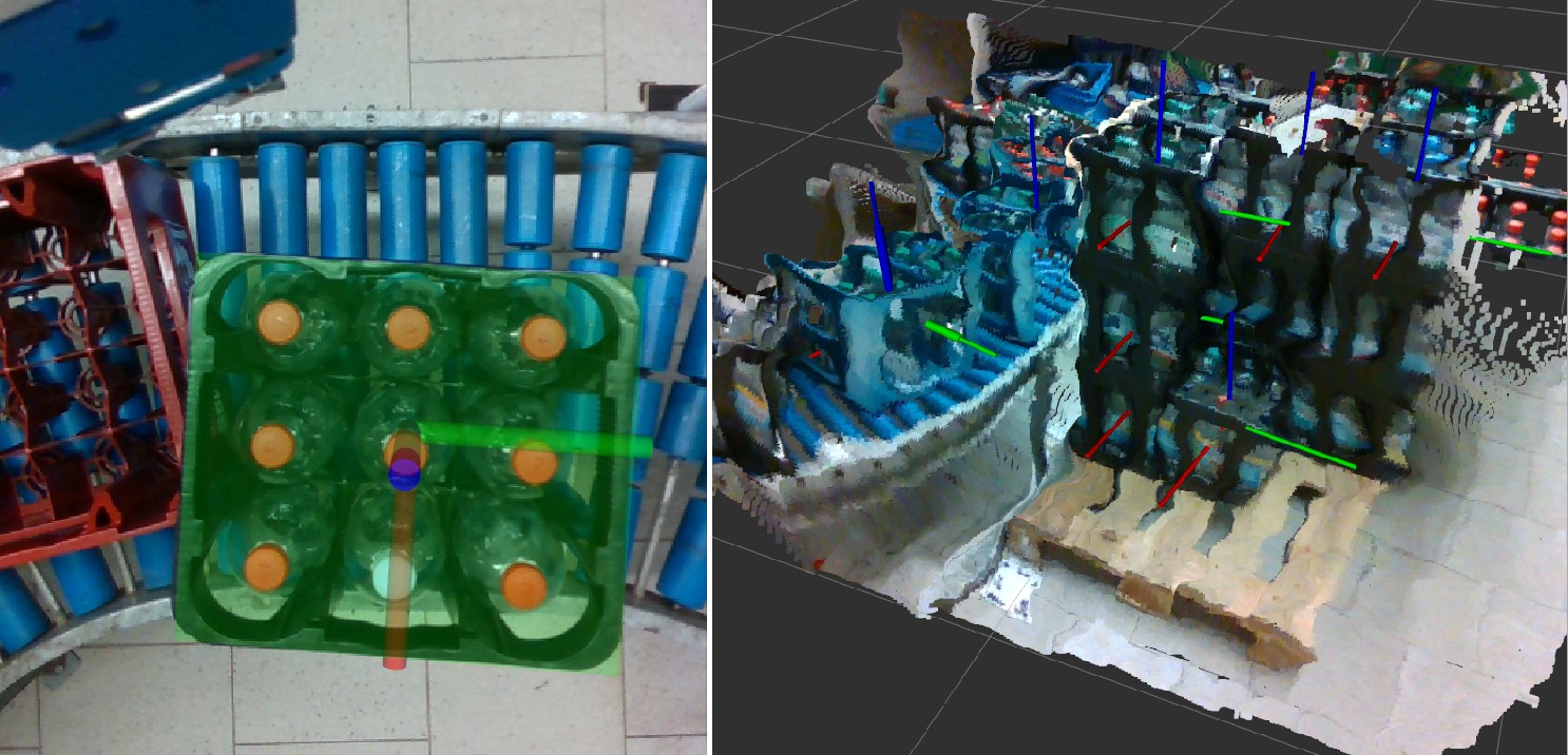
Figure 10: Detection of beverage crates (Intel® RealSense D435)

To facilitate the integration and practical use of our detection system, we developed interfaces for ROS and the Universal Robot platform via URCap-XMLRPC and provide a general REST-API. We used the ROS interface to integrate it on a mobile robot platform and applied it to beverage logistics (Figs. 1 and 10). We also used the XMLRPC interface to integrate it in our ”AI-Picking” lab demonstrator (as shown in the attached video), where we use much smaller pallets and packaging units. There we did not have to train a new model, we simply scaled the whole geometry and worked with an existing model that was trained for euro pallets. With the intention to improve the detection performance and for comparison, we implemented as simple strategy for depth map completion specialized for the depalletizing task. Therefore we used morphological operations to set large and far away areas to the depth value of the wall before we use a classical inpainting method following [36] to fill the remaining small areas (Fig. 11).

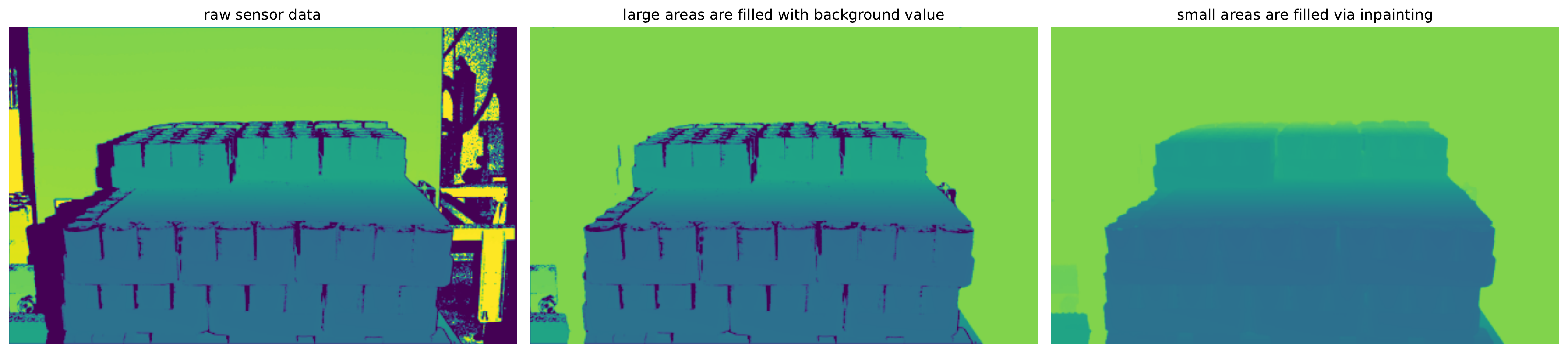
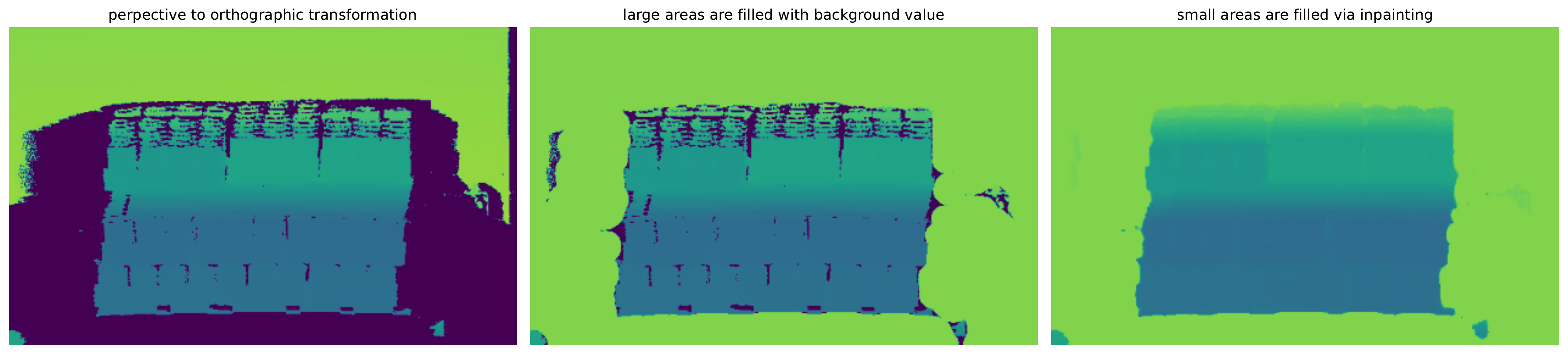
Figure 11: Our depth completion strategy on raw sensor data (top) and the orthographic projection of the raw sensor data (bottom)

V-2 Evaluation on Real-World Data

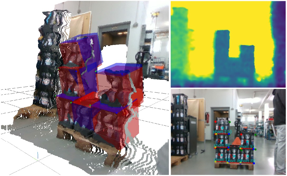
Figure 12: Failure case: bad pose estimations caused by low sensor quality (Intel® RealSense D435); direct regression (red) and based on keypoint regregression (blue)

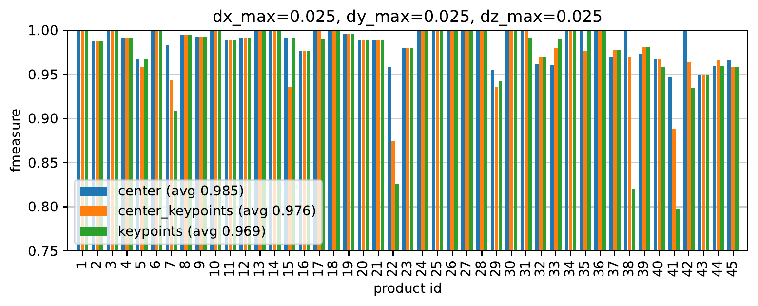
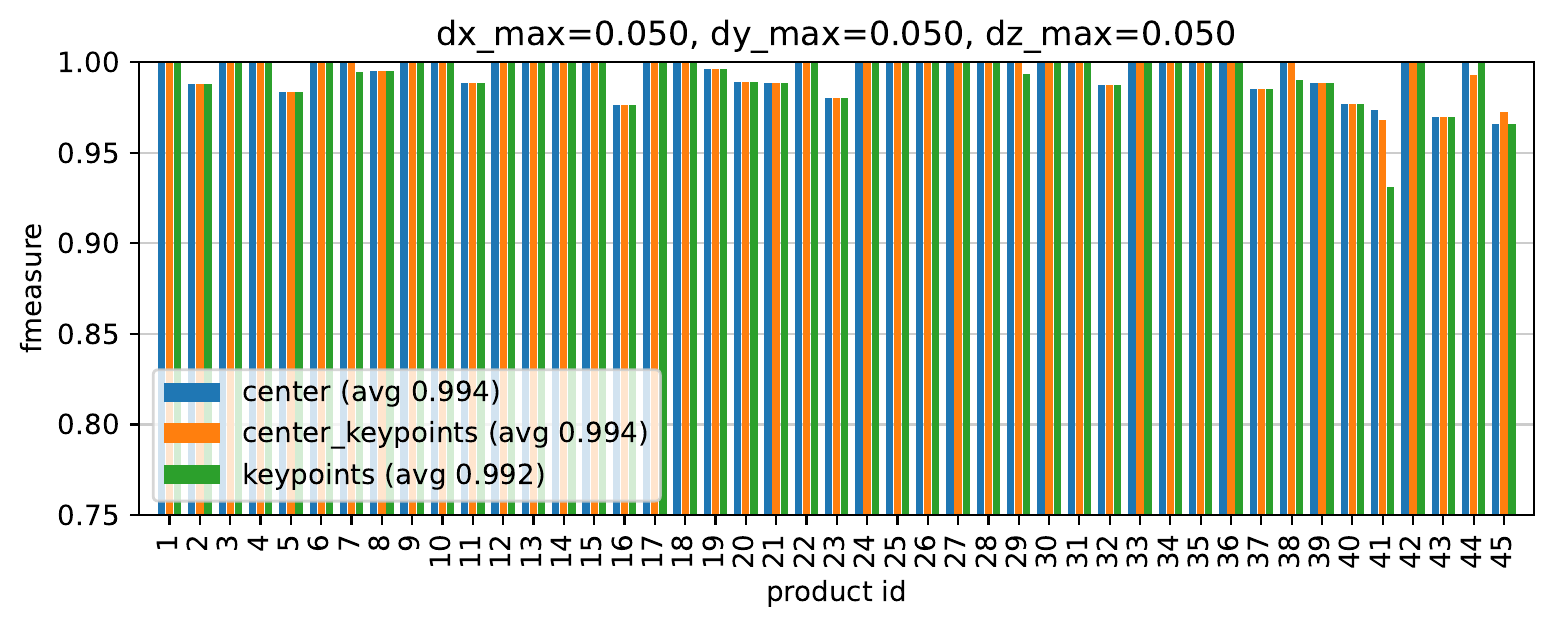
Figure 13: Evaluation on 45 different products with 50 samples per product; maximum permissible deviation 25 mm (top) / 50 mm (bottom)

Due to the poor quality of the Intel® RealSense D435, it made little sense for us to annotate larger amounts of data from this sensor that can be used for evaluation. For the case of the depalettizing task where the box size is known, we got annotations on sensor data from the Zivid One+ Large. With this real world annotations we were able evaluate our system on a wide range of different products. We evaluated it with 50 samples per product on 45 different commercial products (2250 samples in total). Since only the detections in the topmost layer are relevant for the depalletizing task and we only have reliable annotations for this layer, we only detect and evaluate on the topmost layer (8937 instances in total). We used the f-measure (harmonic mean of precision and recall) as primary metric for the evaluation shown in Fig. 13. A detection is counted as true positive if its positional distance in pallet frame does not deviate more than a certain maximal value ($d_{x,\text{max}},d_{y,\text{max}},d_{z,\text{max}}$), the orientation (short, long) is classified correctly and it is no duplicate detection. We evaluated for the direct regression of the box center, the box center constructed from the 3D keypoints and on the bottom-left and bottom-right front keypoints (red line in Figs. 14 and 15, since it is most relevant for picking. With a maximum permissible deviation of 25 mm in $x,y,z$ at an average camera distance of $1.8$ m, we get an average f-measure of 0.985 over all products. The direct regression of the box center location gives the best results for almost all products. We have also done this evaluation with our depth completion strategy from the previous section and found that depth completion roughly decreases the f-measure by 0.01. Closer investigations showed that it fails on large areas without depth information, caused by reflection or transparent materials, which can be better handled by the Partial Convolutions. The increase of the maximum permissible deviation in position from 25 mm to 50 mm shows that the actual detection of packaging units is not an issue, it is mostly a question of position error. We found several causes which require more detailed investigation in future work to further reduce the position error:

1. Inaccuracy of human annotations in the test data

2. Low quality of sensor data resulting from transparency and reflections

3. Small resolution in the model input

4. Synthetic-to-real gap

5. Tolerances of provided box size

6. Deformations of the packaging units

VI Conclusion and Future Work

In this paper, we proposed a unified framework for packaging unit detection and applied it to various scenarios. We also contributed with several novel concepts for improving the training of single-shot object detectors and the post-processing stage in Section III. Resulting from the presented work, directions for further work arise. The proposed BDT, DSSL and certainty prediction should be applied with several generic state-of-the-art object detection frameworks and evaluated on well known benchmarks like MS COCO [37].

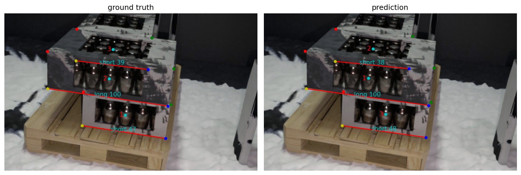
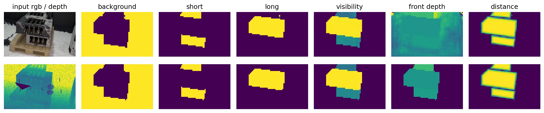
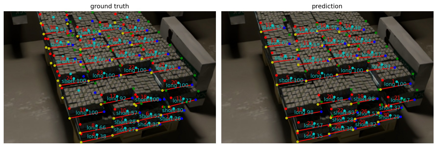
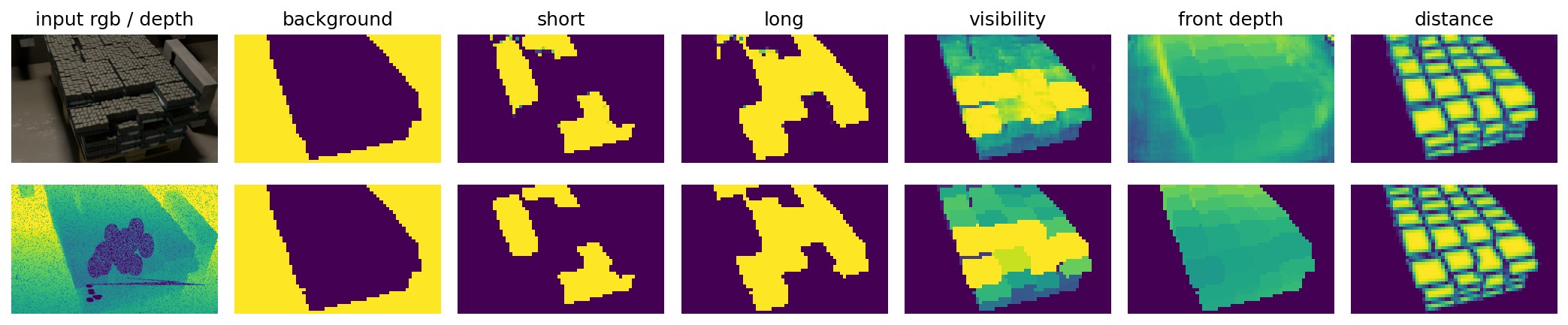
Figure 14: Prediction on generated validation data; only instances with visibility $>0.25$ are shown

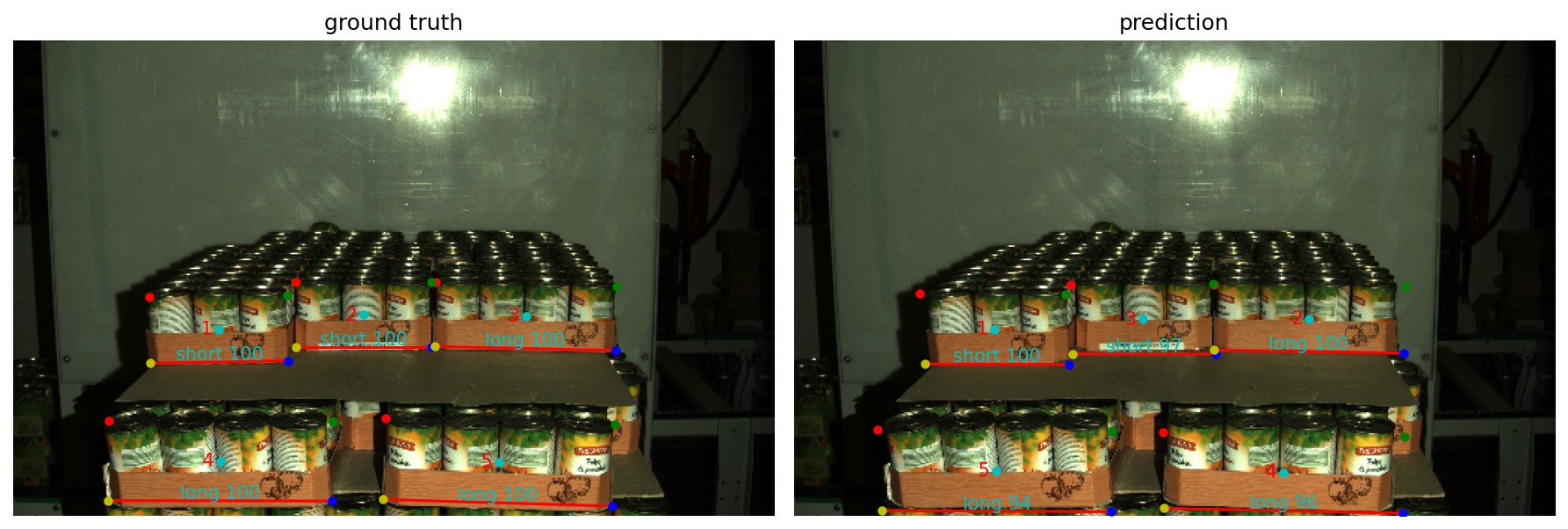
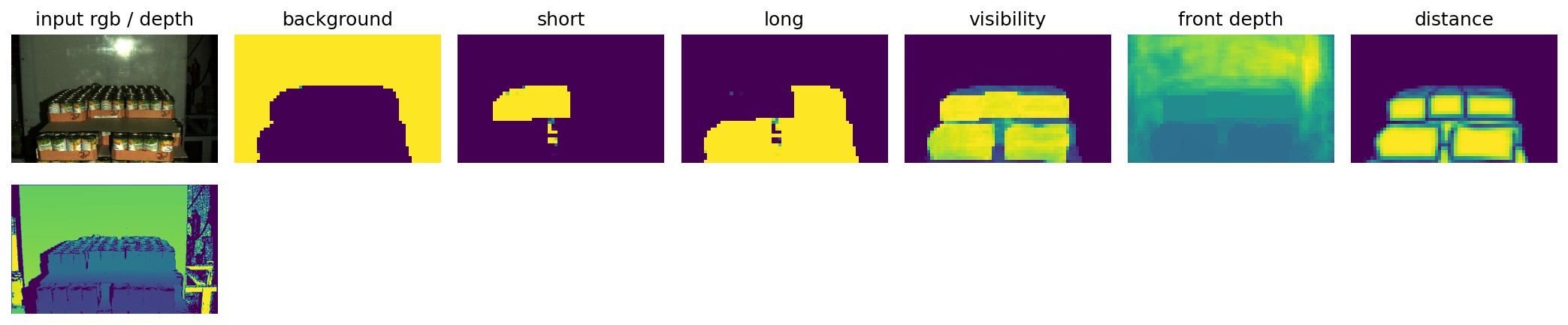
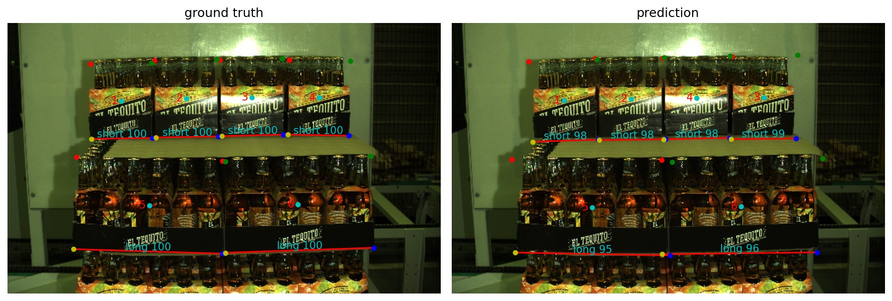
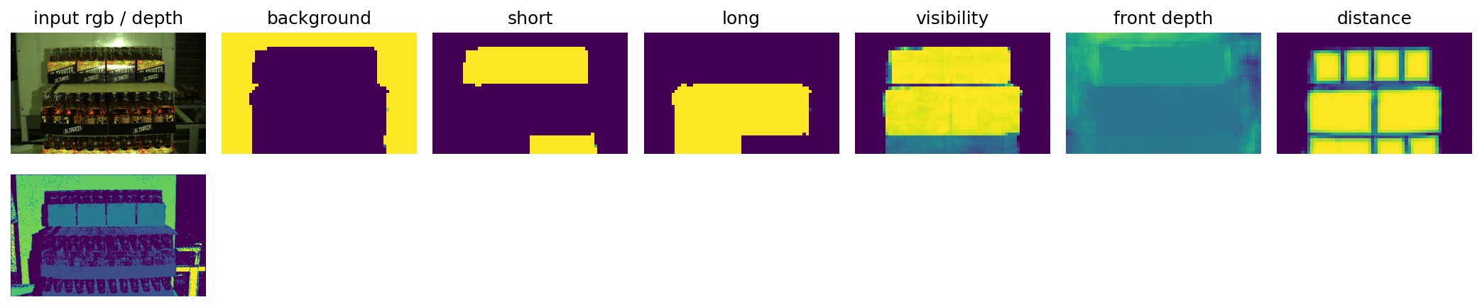
Figure 15: Prediction on real data; only instances with visibility $>0.25$ are shown

References

- [1] H. Muetherich, F. Simons, and A. Verl, “Gripping systems for intralogistics - aiming at the ”swiss army knife” of intralogistics solutions,” in ISR and ROBOTIK, 2010, pp. 1–7.
- [2] S. Hoque, M. Y. Arafat, S. Xu, A. Maiti, and Y. Wei, “A comprehensive review on 3d object detection and 6d pose estimation with deep learning,” IEEE Access, vol. 9, pp. 143 746–143 770, 2021.
- [3] F. Gorschlüter, P. Rojtberg, and T. Pöllabauer, “A survey of 6d object detection based on 3d models for industrial applications,” Journal of Imaging, vol. 8, no. 3, p. 53, 2022.
- [4] R. Monica, J. Aleotti, and D. L. Rizzini, “Detection of parcel boxes for pallet unloading using a 3d time-of-flight industrial sensor,” in IEEE Internat. Conf. on Robotic Computing (IRC), 2020, pp. 314–318.
- [5] J. Aleotti, A. Baldassarri, M. Bonfè, M. Carricato, D. Chiaravalli, and et al., “Toward future automatic warehouses: An autonomous depalletizing system based on mobile manipulation and 3d perception,” Applied Sciences, vol. 11, no. 13, p. 5959, 2021.
- [6] D. Holz, A. Topalidou-Kyniazopoulou, J. Stückler, and S. Behnke, “Real-time object detection, localization and verification for fast robotic depalletizing,” in IROS, 2015, pp. 1459–1466.
- [7] P. Arpenti, R. Caccavale, G. Paduano, G. Andrea Fontanelli, V. Lippiello, L. Villani, and B. Siciliano, “RGB-d recognition and localization of cases for robotic depalletizing in supermarkets,” IEEE Robotics and Automation Letters, vol. 5, no. 4, pp. 6233–6238, 2020.
- [8] J. Li, J. Kang, Z. Chen, F. Cui, and Z. Fan, “A workpiece localization method for robotic de-palletizing based on region growing and PPHT,” IEEE Access, vol. 8, pp. 166 365–166 376, 2020.
- [9] C. Prasse, S. Skibinski, F. Weichert, J. Stenzel, H. Müller, and M. ten Hompel, “Concept of automated load detection for de-palletizing using depth images and RFID data,” in ICCSCE, 2011, pp. 249–254.
- [10] R. Caccavale, P. Arpenti, G. Paduano, A. Fontanellli, V. Lippiello, L. Villani, and B. Siciliano, “A flexible robotic depalletizing system for supermarket logistics,” IEEE Robotics and Automation Letters, vol. 5, no. 3, pp. 4471–4476, 2020.
- [11] W. Liu, D. Anguelov, D. Erhan, C. Szegedy, S. Reed, C.-Y. Fu, and A. C. Berg, “SSD: Single shot MultiBox detector,” arXiv:1512.02325 [cs], vol. 9905, pp. 21–37, 2016.
- [12] A. Bochkovskiy, C.-Y. Wang, and H.-Y. M. Liao, “YOLOv4: Optimal speed and accuracy of object detection,” arXiv:2004.10934 [cs], 2020.
- [13] C.-Y. Wang, A. Bochkovskiy, and H.-Y. M. Liao, “YOLOv7: Trainable bag-of-freebies sets new state-of-the-art for real-time object detectors,” 2022.
- [14] T.-Y. Lin, P. Goyal, R. Girshick, K. He, and P. Dollár, “Focal loss for dense object detection,” arXiv:1708.02002 [cs], 2017.
- [15] A. Shrivastava, A. Gupta, and R. Girshick, “Training region-based object detectors with online hard example mining,” arXiv:1604.03540 [cs], 2016.
- [16] N. Sergievskiy and A. Ponamarev, “Reduced focal loss: 1st place solution to xView object detection in satellite imagery,” arXiv:1903.01347 [cs], 2019.
- [17] X. Lu, C. Ma, B. Ni, X. Yang, I. Reid, and M.-H. Yang, “Deep regression tracking with shrinkage loss,” p. 17, 2018.
- [18] P. J. Huber, “Robust estimation of a location parameter,” The Annals of Mathematical Statistics, vol. 35, no. 1, pp. 73–101, 1964.
- [19] R. Girshick, “Fast r-CNN,” arXiv:1504.08083 [cs], 2015.
- [20] Z. Zheng, P. Wang, W. Liu, J. Li, R. Ye, and D. Ren, “Distance-IoU loss: Faster and better learning for bounding box regression,” arXiv:1911.08287 [cs], 2019.
- [21] Z. Tian, C. Shen, H. Chen, and T. He, “FCOS: Fully convolutional one-stage object detection,” 2019.
- [22] S. Wu, X. Li, and X. Wang, “IoU-aware single-stage object detector for accurate localization,” 2020.
- [23] F. Chollet, “Xception: Deep learning with depthwise separable convolutions,” arXiv:1610.02357 [cs], 2016.
- [24] A. G. Howard, M. Zhu, B. Chen, D. Kalenichenko, W. Wang, T. Weyand, M. Andreetto, and H. Adam, “MobileNets: Efficient convolutional neural networks for mobile vision applications,” arXiv:1704.04861 [cs], 2017.
- [25] M. Sandler, A. Howard, M. Zhu, A. Zhmoginov, and L.-C. Chen, “MobileNetV2: Inverted residuals and linear bottlenecks,” 2018.
- [26] R. Liu, J. Lehman, P. Molino, F. P. Such, E. Frank, A. Sergeev, and J. Yosinski, “An intriguing failing of convolutional neural networks and the CoordConv solution,” arXiv:1807.03247 [cs, stat], 2018.
- [27] J. Uhrig, N. Schneider, L. Schneider, U. Franke, T. Brox, and A. Geiger, “Sparsity invariant CNNs,” arXiv:1708.06500 [cs], 2017.
- [28] G. Liu, F. A. Reda, K. J. Shih, T.-C. Wang, A. Tao, and B. Catanzaro, “Image inpainting for irregular holes using partial convolutions,” 2018.
- [29] S. Hinterstoisser, O. Pauly, H. Heibel, M. Marek, and M. Bokeloh, “An annotation saved is an annotation earned: Using fully synthetic training for object instance detection,” 2019.
- [30] T. Hodan, V. Vineet, R. Gal, E. Shalev, J. Hanzelka, T. Connell, P. Urbina, S. N. Sinha, and B. Guenter, “Photorealistic image synthesis for object instance detection,” 2019.
- [31] J. Devlin, M.-W. Chang, K. Lee, and K. Toutanova, “BERT: Pre-training of deep bidirectional transformers for language understanding,” arXiv:1810.04805 [cs], 2019.
- [32] K. He, X. Chen, S. Xie, Y. Li, P. Dollár, and R. Girshick, “Masked autoencoders are scalable vision learners,” 2021.
- [33] N. Srivastava, G. E. Hinton, A. Krizhevsky, I. Sutskever, and R. Salakhutdinov, “Dropout: a simple way to prevent neural networks from overfitting.” Journal of machine learning research, vol. 15, no. 1, pp. 1929–1958, 2014.
- [34] T. Strutz, “The distance transform and its computation,” 2021.
- [35] The OpenCV Reference Manual, 2nd ed. Itseez, 2014.
- [36] A. Telea, “An image inpainting technique based on the fast marching method,” Journal of Graphics Tools, vol. 9, no. 1, pp. 23–34, 2004.
- [37] T.-Y. Lin, M. Maire, S. Belongie, L. Bourdev, R. Girshick, J. Hays, P. Perona, D. Ramanan, C. L. Zitnick, and P. Dollár, “Microsoft COCO: Common objects in context,” arXiv:1405.0312 [cs], 2014.