The Asymptotic Properties of the One-Sample Spatial Rank Methods

Abstract

For a set of $p$-variate data points $\mathbf{y}_{1},\ldots,\mathbf{y}_{n}$, there are several versions of multivariate median and related multivariate sign test proposed and studied in the literature. In this paper we consider the asymptotic properties of the multivariate extension of the Hodges-Lehmann (HL) estimator, the spatial HL-estimator, and the related test statistic. The asymptotic behavior of the spatial HL-estimator and the related test statistic when $n$ tends to infinity are collected, reviewed, and proved, some for the first time though being used already for a longer time. We also derive the limiting behavior of the HL-estimator when both the sample size $n$ and the dimension $p$ tend to infinity.

Keywords Spatial HL-estimator  $\cdot$ spatial median  $\cdot$ spatial signed-rank test

1 Introduction

For a set of $p$-variate data points $\mathbf{y}_{1},\ldots,\mathbf{y}_{n}$, there are several versions of multivariate median and related multivariate sign test proposed and studied in the literature. For some general reviews, see Small (1990) and Oja (2013), for example. The so-called spatial median which minimizes the sum $\sum_{i=1}^{n}\|\mathbf{y}_{i}-\boldsymbol{\mu}\|$ with the Euclidean norm $\|\mathbf{y}\|=({\mathbf{y}}^{\top}\mathbf{y})^{1/2}$ has a very long history started by Gini & Galvani (1929) and Haldane (1948). Brown (1983) has developed many of the properties of the spatial median. Taking the gradient of the objective function, one sees that the multivariate sample spatial median ${\hat{\boldsymbol{\mu}}_{\mathrm{SM}}}$ solves the equation $\sum_{i=1}^{n}\mathbf{u}(\mathbf{y}_{i}-\hat{\boldsymbol{\mu}})=\mathbf{0}$ with the spatial sign

$$\mathbf{u}(\mathbf{y})=\begin{cases}\mathbf{y}/\|\mathbf{y}\|,&\text{when $\mathbf{y}\neq\mathbf{0}$},\\ \mathbf{0},&\text{when $\mathbf{y}=\mathbf{0}$}.\end{cases}$$

The spatial sign test statistic $\sum_{i=1}^{n}\mathbf{u}(\mathbf{y}_{i})$ for $H_{0}:{\color[rgb]{0,0,0}{{\boldsymbol{\mu}_{\mathrm{SM}}}}}=\mathbf{0}$. was considered by Möttönen & Oja (1995), for example. See also Oja (Chapter 6 2010).

In this paper, we consider a multivariate extension of the popular Hodges-Lehmann (HL) estimator (Hodges & Lehmann, 1963), the spatial HL-estimator ${\color[rgb]{0,0,0}{{\hat{\boldsymbol{\mu}}_{\mathrm{HL}}}}}$, which minimizes the sum $\sum_{i<j}\|(\mathbf{y}_{i}+\mathbf{y}_{j})/2-\boldsymbol{\mu}\|$ and is closely related to the multivariate spatial signed-rank test statistic $\sum_{i<j}\mathbf{u}((\mathbf{y}_{i}+\mathbf{y}_{j})/2)$ for $H_{0}:{\color[rgb]{0,0,0}{{\boldsymbol{\mu}_{\mathrm{HL}}}}}=\mathbf{0}$. See Chaudhuri (1992) and Möttönen & Oja (1995) for early studies of these statistics. Other well-known multivariate extensions are the vector of marginal HL-estimators (Puri & Sen, 1971) and the HL-estimator based on Oja signed-ranks (Hettmansperger et al., 1997). Hallin & Paindaveine (2002) constructed multivariate signed-rank test statistics that are based on standardized spatial signs or Randles’ interdirections (Randles, 1989) and the ranks of Mahalanobis distances from the origin. See also Möttönen et al. (2005) for multivariate generalized spatial signed-rank methods.

Möttönen et al. (2010) provided the detailed results on the limiting behavior of the spatial median and its affine equivariant modification, so called transformation-retransformation estimator, when $n\to\infty$. In this paper we collect and review in the same way the behavior of the spatial Hodges-Lehmann estimator when $n\to\infty$. Many of the results and auxiliary results can be collected from Arcones (1998); Bai et al. (1990); Chaudhuri (1992); Möttönen & Oja (1995).

In this article we also study the limiting behavior of the HL-estimator when both sample size $n\to\infty$ and the dimension $p\to\infty$. Zou et al. (2014) presented an asymptotic expansion of the spatial median under elliptical distributions with identity scatter matrix and applied this expansion to a sign-based test for the sphericity. Li & Xu (2022) provide some results for the asymptotic behavior of sample spatial median under elliptical distributions when $p$ diverges to infinity at the same rate as $n$. See also Cheng et al. (2019), Feng & Sun (2016) and Feng et al. (2016).

The paper is structured as follows. In Section 2 we recall the basic properties of the spatial median and the transformation-retransformation spatial median. In Sections 3 and 4 we consider the asymptotic properties of the spatial HL-estimator and the transformation-retransformation HL-estimator. In Section 5 the properties of the spatial signed-rank test are reviewed. In Section 6 we study the limiting behavior of the HL-estimator in high-dimensional regime, i.e. when both sample size $n$ and dimension $p$ tend to infinity. The proofs of all the theorems and lemmas are presented in the Appendix.

2 Review of the spatial median and the transformation-retransformation spatial median

In this section we review the properties of the spatial median and the transformation-retransformation spatial median. The corresponding proofs of the lemmas and theorems are presented in Möttönen et al. (2010).

Let $\mathbf{y}$ be a $p$-variate random vector with cdf $F$ and $p>1$. The spatial median of $F$ minimizes the objective function

$$d_{1}(\boldsymbol{\mu})=\mathbb{E}\{\|\mathbf{y}-\boldsymbol{\mu}\|-\|\mathbf{y}\|\}.$$

Note that, as $|\|\mathbf{y}-\boldsymbol{\mu}\|-\|\mathbf{y}\||\leq\|\boldsymbol{\mu}\|$, the expectation always exists. Let ${\mathbf{y}}_{1},\ldots,{\mathbf{y}}_{n}$ be a random sample from a $p$-variate distribution $F$ and $\mathbf{Y}=(\mathbf{y}_{1},\ldots,\mathbf{y}_{n})^{\top}$ be an $n\times p$ matrix of the $n$ observation vectors. The multivariate sample spatial median $\hat{\boldsymbol{\mu}}_{\mathrm{SM}}=\hat{\boldsymbol{\mu}}_{\mathrm{SM}}(\mathbf{Y})$ minimizes the objective function

$$d_{1n}(\boldsymbol{\mu})=\frac{1}{n}\sum_{i=1}^{n}\{\|\mathbf{y}_{i}-\boldsymbol{\mu}\|-\|\mathbf{y}_{i}\|\}.$$

We consider next the distribution of the multivariate sample spatial median ${\color[rgb]{0,0,0}{{\hat{\boldsymbol{\mu}}_{\mathrm{SM}}}}}$ under the following assumption:

Assumption 1

(a) The density of $\mathbf{y}_{i}$ is continuous and bounded in an open neighborhood of the origin. (b) The spatial median of $\mathbf{y}_{i}$ is unique ${\color[rgb]{0,0,0}{{\boldsymbol{\mu}_{\mathrm{SM}}}}}=\mathbf{0}$.

We define the following functions

$$\mathbf{u}(\mathbf{y}) = \|\mathbf{y}\|^{-1}\mathbf{y},\ \ \ \mathbf{A}(\mathbf{y})=\|\mathbf{y}\|^{-1}\left[\mathbf{I}_{p}-\|\mathbf{y}\|^{-2}\mathbf{y}\mathbf{y}^{\top}\right],\ \ \ \mbox{and}\ \ \$$

$$\mathbf{B}(\mathbf{y}) = \mathbf{u}(\mathbf{y})\mathbf{u}(\mathbf{y})^{\top}=\|\mathbf{y}\|^{-2}\mathbf{y}\mathbf{y}^{\top},$$

for $\mathbf{y}\neq\mathbf{0}$. For $\mathbf{y}=\mathbf{0}$ we set $\mathbf{u}(\mathbf{0})=\mathbf{0}$, $\mathbf{A}(\mathbf{0})=\mathbf{0}$ and $\mathbf{B}(\mathbf{0})=\mathbf{0}$. Note that $\mathbf{u}(\mathbf{y})=\nabla\|\mathbf{y}\|$ is the spatial sign vector of vector $\mathbf{y}$ (the gradient vector of $\|\mathbf{y}\|$) and $\mathbf{A}(\mathbf{y})=\nabla^{2}\|\mathbf{y}\|$ is the Hessian matrix of $\|\mathbf{y}\|$. We also define the sample statistics

$$\hat{\mathbf{A}}=\frac{1}{n}\sum_{i=1}^{n}\mathbf{A}(\mathbf{y}_{i})\ \ \ \mbox{and}\ \ \ \hat{\mathbf{B}}=\frac{1}{n}\sum_{i=1}^{n}\mathbf{B}(\mathbf{y}_{i}).$$

Theorem 1

Let $\mathbf{y}_{1},\ldots,\mathbf{y}_{n}$ be iid observations from a distribution satisfying Assumption 1. Then

$${\hat{\boldsymbol{\mu}}_{\mathrm{SM}}}\stackrel{{\scriptstyle a.s.}}{{\longrightarrow}}\mathbf{0}.$$

Theorem 2

Let $\mathbf{y}_{1},\ldots,\mathbf{y}_{n}$ be iid observations from a distribution satisfying Assumption 1. Then

$$\sqrt{n}{\color[rgb]{0,0,0}{{\hat{\boldsymbol{\mu}}_{\mathrm{SM}}}}}\stackrel{{\scriptstyle d}}{{\longrightarrow}}N_{p}(\mathbf{0},\mathbf{A}^{-1}\mathbf{B}\mathbf{A}^{-1}),$$

where $\mathbf{A}=\mathbb{E}\{\mathbf{A}(\mathbf{y}_{i})\}$ and $\mathbf{B}=\mathbb{E}\{\mathbf{B}(\mathbf{y}_{i})\}$.

Theorem 3

Let $\mathbf{y}_{1},\ldots,\mathbf{y}_{n}$ be a iid observations from a distribution satisfying Assumption 1. Then

$$\hat{\mathbf{A}}\stackrel{{\scriptstyle{\mathbb{P}}}}{{\longrightarrow}}\mathbf{A}\ \ \ \mbox{and}\ \ \ \hat{\mathbf{B}}\stackrel{{\scriptstyle{\mathbb{P}}}}{{\longrightarrow}}\mathbf{B}.$$

Theorems 2 and 3 imply that we can approximate the covariance matrix of ${\color[rgb]{0,0,0}{{\hat{\boldsymbol{\mu}}_{\mathrm{SM}}}}}$ by $\frac{1}{n}\hat{\mathbf{A}}^{-1}\hat{\mathbf{B}}\hat{\mathbf{A}}^{-1}$.

To compute the spatial median ${\hat{\boldsymbol{\mu}}_{\mathrm{SM}}}$ there are several algorithms proposed in the literature. For example, the algorithms of Vardi & Zhang (2000), Hössjer & Croux (1995), Fritz et al. (2012) and Kent et al. (2015). See also Oja (2010) and Nordhausen & Oja (2011).

The spatial median ${\color[rgb]{0,0,0}{{\hat{\boldsymbol{\mu}}_{\mathrm{SM}}}}}$ is rotation and shift equivariant, that is,

$${\color[rgb]{0,0,0}{{\hat{\boldsymbol{\mu}}_{\mathrm{SM}}}}}(\mathbf{Y}\mathbf{O}^{\top}+\mathbf{1}_{n}{\mathbf{a}}^{\top})=\mathbf{O}{\color[rgb]{0,0,0}{{\hat{\boldsymbol{\mu}}_{\mathrm{SM}}}}}(\mathbf{Y})+\mathbf{a}$$

for all orthogonal $p\times p$ matrices $\mathbf{O}$ and for all $p\times 1$ vectors $\mathbf{a}$. It is not affine equivariant, however, as ${\color[rgb]{0,0,0}{{\hat{\boldsymbol{\mu}}_{\mathrm{SM}}}}}(\mathbf{Y}\mathbf{D}^{\top})$ and $\mathbf{D}{\color[rgb]{0,0,0}{{\hat{\boldsymbol{\mu}}_{\mathrm{SM}}}}}(\mathbf{Y})$ may be different for $p\times p$ diagonal matrices $\mathbf{D}$. We get an affine equivariant version of the spatial median by using a transformation-retransformation (TR) method. See Chakraborty et al. (1998). The transformation-retransformation method takes advantage of the properties of scatter matrices.

Definition 1

Let $\mathbf{Y}=(\mathbf{y}_{1},\ldots,\mathbf{y}_{n})^{\top}$ be an $n\times p$ data matrix. A $p\times p$ matrix (a sample statistic) $\mathbf{S}(\mathbf{Y})$ is a scatter matrix if it is symmetric, non-negative definite and affine equivariant in the sense

$$\mathbf{S}(\mathbf{Y}{\mathbf{B}}^{\top}+\mathbf{1}_{n}{\mathbf{a}}^{\top})=\mathbf{B}\mathbf{S}(\mathbf{Y}){\mathbf{B}}^{\top}$$

for all data matrices $\mathbf{Y}$, all nonsingular $p\times p$ matrices $\mathbf{B}$ and all $p\times 1$ vectors $\mathbf{a}$.

For some functionals $\mathbf{S}(\mathbf{Y})$ it only holds that $\mathbf{S}(\mathbf{Y}{\mathbf{B}}^{\top}+\mathbf{1}_{n}{\mathbf{a}}^{\top})\propto\mathbf{B}\mathbf{S}(\mathbf{Y}){\mathbf{B}}^{\top}$ and $\mathbf{S}$ is then often called a shape matrix. In the following we use the word scatter also for shape matrices as they both can be similarly used for our purposes. See Frahm (2009) for a detailed discussion on affine equivariant shape matrices.

Let $\mathbf{S}$ be a positive definite scatter matrix. Then our transformation matrix is a symmetric matrix ${\mathbf{S}}^{-1/2}$ satisfying ${\mathbf{S}}^{-1/2}\ \mathbf{S}\ {\mathbf{S}}^{-1/2}=\mathbf{I}_{p}$ and the retransformation matrix $\mathbf{S}^{1/2}$ is its symmetric inverse. Another possibility is to use the transformation matrix to invariant coordinates and its inverse to transform back, see Tyler et al. (2009) and Ilmonen et al. (2012). The transformation-retransformation procedure is then as follows.

(1)

Take any scatter matrix $\mathbf{S}=\mathbf{S}(\mathbf{Y})$

(2)

Standardize the data matrix: ${\mathbf{Y}}^{*}=\mathbf{Y}({\mathbf{S}}^{-1/2})^{\top}$

(3)

Find the spatial median for the standardized data matrix: ${\color[rgb]{0,0,0}{{\hat{\boldsymbol{\mu}}_{\mathrm{SM}}}}}({\mathbf{Y}}^{*})$

(4)

Retransform the estimator: ${\color[rgb]{0,0,0}{{\hat{\boldsymbol{\mu}}_{\mathrm{TRSM}}}}}(\mathbf{Y})={\mathbf{S}}^{1/2}{\color[rgb]{0,0,0}{{\hat{\boldsymbol{\mu}}_{\mathrm{SM}}}}}({\mathbf{Y}}^{*}).$

It can be easily seen that the transformation-retransformation estimator ${\color[rgb]{0,0,0}{{\hat{\boldsymbol{\mu}}_{\mathrm{TRSM}}}}}(\mathbf{Y})$ is affine equivariant, i.e.

$${\color[rgb]{0,0,0}{{\hat{\boldsymbol{\mu}}_{\mathrm{TRSM}}}}}(\mathbf{Y}\mathbf{B}^{\top}+\mathbf{1}_{n}{\mathbf{a}}^{\top})=\mathbf{B}{\color[rgb]{0,0,0}{{\hat{\boldsymbol{\mu}}_{\mathrm{TRSM}}}}}(\mathbf{Y})+\mathbf{a}$$

for all nonsingular $p\times p$ matrices $\mathbf{B}$ and all $p\times 1$ vectors $\mathbf{a}$.

For the transformation-retransformation spatial median a scatter matrix is needed. One possible choice is the Tyler’s shape matrix. Tyler’s shape matrix is explained in detail in Tyler (1987) and reviewed in Taskinen et al. (2023). A problem with Tyler’s shape matrix is that it requires a location value in order to center the data. For a joint estimation of the spatial median and Tyler’s shape matrix one can use the Hettmansperger-Randles (HR) algorithm (Hettmansperger & Randles, 2002). We assume (without loss of generality) that the population value of $\mathbf{S}$ is $\mathbf{I}_{p}$, and that $\mathbf{S}=\mathbf{S}(\mathbf{Y})$ is a $\sqrt{n}$-consistent estimator of $\mathbf{I}_{p}$. The Hettmansperger-Randles estimator of location and scatter are then defined in the following way.

Definition 2

Let ${\boldsymbol{\mu}}$ be a $p\times 1$ vector and $\mathbf{S}$ a symmetric positive definite $p\times p$ matrix, and define ${\mathbf{e}}_{i}={\mathbf{S}}^{-1/2}(\mathbf{y}_{i}-{\boldsymbol{\mu}})$, $i=1,\ldots,n$. The Hettmansperger–Randles (HR) estimator of location and scatter are the values of ${\boldsymbol{\mu}}$ and $\mathbf{S}$ which simultaneously satisfy

$$\frac{1}{n}\sum_{i=1}^{n}\mathbf{u}({\mathbf{e}}_{i})=\mathbf{0}\ \ \text{and}\ \ \frac{1}{n}\sum_{i=1}^{n}\mathbf{u}({\mathbf{e}}_{i})\mathbf{u}({\mathbf{e}}_{i})^{\top}=\frac{1}{p}\mathbf{I}_{p}.$$

The following asymptotic result was proved by Möttönen et al. (2010).

Theorem 4

Let $\mathbf{Y}=(\mathbf{y}_{1},\ldots,\mathbf{y}_{n})^{\top}$ be a random sample from a symmetric distribution around zero satisfying Assumption 1. Assume also that scatter matrix $\mathbf{S}=\mathbf{S}(\mathbf{Y})$ satisfies $\sqrt{n}(\mathbf{S}-\mathbf{I}_{p})=O_{{\mathbb{P}}}(1)$. Then $\sqrt{n}{\color[rgb]{0,0,0}{{\hat{\boldsymbol{\mu}}_{\mathrm{TRSM}}}}}(\mathbf{Y})$ and $\sqrt{n}{\color[rgb]{0,0,0}{{\hat{\boldsymbol{\mu}}_{\mathrm{SM}}}}}(\mathbf{Y})$ have the same limiting distribution.

For a detailed comparison of the spatial median and transformation-retransformation spatial median under ellipticity see Magyar & Tyler (2011).

3 The multivariate spatial HL-estimator

In a univariate context, the pseudo-median of a random variable $y$ with cdf $F$ is defined as the median of $(y_{1}+y_{2})/2$, where $y_{1}$ and $y_{2}$ are independent copies of $y$. Hodges & Lehmann (1963) and Sen (1963) suggested independently an estimator for the pseudo-median which is known nowadays as the Hodges-Lehmann estimator. We consider in the following the corresponding concept in a multivariate setting.

Let $\mathbf{y}$ be a $p$-variate random vector with cdf $F$ and $p>1$. The spatial Hodges-Lehmann location center of $F$ minimizes the objective function

$$d_{2}(\boldsymbol{\mu})=\mathbb{E}\left\{\left\|\frac{\mathbf{y}_{1}+\mathbf{y}_{2}}{2}-\boldsymbol{\mu}\right\|-\left\|\frac{\mathbf{y}_{1}+\mathbf{y}_{2}}{2}\right\|\right\},$$

where $\mathbf{y}_{1}$ and $\mathbf{y}_{2}$ are independent random vectors from $F$. See Chaudhuri (1992) and Möttönen & Oja (1995). As in the spatial median case, the expectation always exists since the expression between the braces is always bounded.

Let $\mathbf{y}_{1},\ldots,\mathbf{y}_{n}$ be a random sample from a $p$-variate distribution $F$. The multivariate spatial Hodges-Lehmann estimator of the location center ${\boldsymbol{\mu}_{\mathrm{HL}}}$ is defined as the spatial median of pairwise means, i.e. the Walsh averages,

$$\mathbf{z}_{i,j}=\frac{\mathbf{y}_{i}+\mathbf{y}_{j}}{2},\ \ \ 1\leq i<j\leq n.$$

The sample spatial Hodges-Lehmann estimator ${\hat{\boldsymbol{\mu}}_{\mathrm{HL}}}$ thus minimizes the criterion function

$$d_{2n}(\boldsymbol{\mu})={\binom{n}{2}}^{-1}\sum_{i<j}\left\{\left\|\frac{\mathbf{y}_{i}+\mathbf{y}_{j}}{2}-\boldsymbol{\mu}\right\|-\left\|\frac{\mathbf{y}_{i}+\mathbf{y}_{j}}{2}\right\|\right\}={\binom{n}{2}}^{-1}\sum_{i<j}\left\{\left\|\mathbf{z}_{i,j}-\boldsymbol{\mu}\right\|-\left\|\mathbf{z}_{i,j}\right\|\right\}{\color[rgb]{0,0,0}{{.}}}$$

We consider next the distribution of the multivariate spatial Hodges-Lehmann estimator ${\hat{\boldsymbol{\mu}}_{\mathrm{HL}}}$ and spatial rank test statistic under mild assumptions. For the asymptotic theory we assume that

Assumption 2

(a) The density of $\mathbf{z}_{i,j}$ is continuous and bounded. (b) The spatial median of $\mathbf{z}_{i,j}$ is unique ${\color[rgb]{0,0,0}{{\boldsymbol{\mu}_{\mathrm{HL}}}}}=\mathbf{0}$.

Theorem 5

Let $\mathbf{z}_{i,j}$, $1\leq i<j\leq n$, be observations from a distribution satisfying Assumption 2. Then

$${\hat{\boldsymbol{\mu}}_{\mathrm{HL}}}\stackrel{{\scriptstyle a.s.}}{{\longrightarrow}}\mathbf{0}.$$

Theorem 6

Let $\mathbf{z}_{i,j}$, $1\leq i<j\leq n$, be observations from a distribution satisfying Assumption 2. Then

$$\sqrt{n}{\color[rgb]{0,0,0}{{\hat{\boldsymbol{\mu}}_{\mathrm{HL}}}}}\stackrel{{\scriptstyle d}}{{\longrightarrow}}N_{p}(\mathbf{0},4\mathbf{A}^{-1}\mathbf{B}\mathbf{A}^{-1}),$$

where

$$\mathbf{A}=\mathbb{E}\{\|\mathbf{z}_{1,2}\|^{-1}(\mathbf{I}_{p}-\|\mathbf{z}_{1,2}\|^{-2}\mathbf{z}_{1,2}\mathbf{z}_{1,2}^{\top})\}\ \ \text{and}\ \ \mathbf{B}=\mathbb{E}\{(\|\mathbf{z}_{1,2}\|^{-1}\mathbf{z}_{1,2})(\|\mathbf{z}_{2,3}\|^{-1}\mathbf{z}_{2,3}^{\top})\}.$$

Note that the matrices $\mathbf{A}$ and $\mathbf{B}$ are computed using dependent Walsh averages

$$\mathbf{z}_{1,2}=\frac{\mathbf{y}_{1}+\mathbf{y}_{2}}{2}\ \ \text{and}\ \ \mathbf{z}_{2,3}=\frac{\mathbf{y}_{2}+\mathbf{y}_{3}}{2},$$

where $\mathbf{y}_{1}$, $\mathbf{y}_{2}$ and $\mathbf{y}_{3}$ are independent copies from $F$. The proof of Theorem 6 implies that the covariance matrix of ${\color[rgb]{0,0,0}{{\hat{\boldsymbol{\mu}}_{\mathrm{HL}}}}}$ can be approximated by

$$\frac{1}{n}4\hat{\mathbf{A}}^{-1}\hat{\mathbf{B}}\hat{\mathbf{A}}^{-1},$$

where $\hat{\mathbf{A}}={\binom{n}{2}}^{-1}\sum_{i<j}\|\mathbf{z}_{i,j}\|^{-1}(\mathbf{I}_{p}-\|\mathbf{z}_{i,j}\|^{-2}\mathbf{z}_{i,j}\mathbf{z}_{i,j}^{\top})$ and
$\hat{\mathbf{B}}={\binom{n}{3}}^{-1}\sum_{i<j<k}(\|\mathbf{z}_{i,j}\|^{-1}\mathbf{z}_{i,j})(\|\mathbf{z}_{j,k}\|^{-1}\mathbf{z}_{j,k}^{\top}).$

4 Transformation-retransformation HL-estimator

As the spatial median, the spatial HL-estimator given in Section 3 is only shift and rotation equivariant. Also in this case an affine equivariant version can be found by using transformation-retransformation method (Chakraborty et al., 1998). The procedure is as follows.

(1)

Take any scatter matrix $\mathbf{S}=\mathbf{S}(\mathbf{Y})$

(2)

Standardize the data matrix: ${\mathbf{Y}}^{*}=\mathbf{Y}({\mathbf{S}}^{-1/2})^{\top}$

(3)

Find the spatial HL-estimator for the standardized data matrix: ${\hat{\boldsymbol{\mu}}_{\mathrm{HL}}}({\mathbf{Y}}^{*})$

(4)

Retransform the estimator: ${\hat{\boldsymbol{\mu}}_{\mathrm{TRHL}}}(\mathbf{Y})={\mathbf{S}}^{1/2}{\hat{\boldsymbol{\mu}}_{\mathrm{HL}}}({\mathbf{Y}}^{*}).$

For the transformation-retransformation Hodges-Lehmann estimator the signed-rank shape matrix seems the most natural transformation matrix. The Hettmansperger-Randles type simultaneous estimators of location and scatter can be defined in the same way as in the spatial median case:

Definition 3

Let ${\boldsymbol{\mu}}$ be a $p\times 1$ vector and $\mathbf{S}$ a symmetric positive definite $p\times p$ matrix, and define ${\mathbf{e}}_{i}={\mathbf{S}}^{-1/2}(\mathbf{y}_{i}-{\boldsymbol{\mu}})$, $i=1,\ldots,n$. The simultaneous estimators of location and scatter are the values of ${\boldsymbol{\mu}}$ and $\mathbf{S}$ for which

$$\frac{1}{n}\sum_{i=1}^{n}\hat{\mathbf{q}}({\mathbf{e}}_{i})=\mathbf{0}\ \ \text{and}\ \ \frac{1}{n}\sum_{i=1}^{n}\hat{\mathbf{q}}({\mathbf{e}}_{i})\hat{\mathbf{q}}({\mathbf{e}}_{i})^{\top}\ \propto\ \mathbf{I}_{p},$$

where $\hat{\mathbf{q}}(\mathbf{e})=\frac{1}{n}\sum_{i=1}^{n}\mathbf{u}((\mathbf{e}_{i}+\mathbf{e})/2)$ is the estimated signed-rank function.

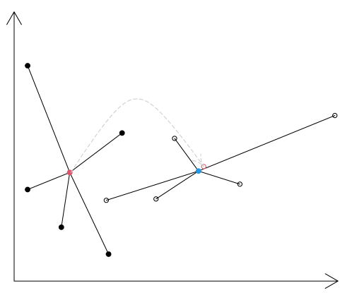
Figure 1: Visualization of effect of the non-affine equivariance of the spatial Hodges-Lehmann estimator. The five solid points have as spatial Hodges-Lehmann estimator the solid red point. Using an affine transformation to these points yields the non-solid points and one can see that the Hodges-Lehmann estimator based on the five transformed points, plotted in blue differs from the transformed original estimate.

Theorem 7

Let $\mathbf{Y}=(\mathbf{y}_{1},\ldots,\mathbf{y}_{n})^{\top}$ be a random sample from a symmetric distribution satisfying Assumption 2. Assume also that scatter matrix $\mathbf{S}=\mathbf{S}(\mathbf{Y})$ satisfies $\sqrt{n}(\mathbf{S}-\mathbf{I}_{p})=O_{{\mathbb{P}}}(1)$. Then $\sqrt{n}{\color[rgb]{0,0,0}{{\hat{\boldsymbol{\mu}}_{\mathrm{TRHL}}}}}(\mathbf{Y})$ and $\sqrt{n}{\color[rgb]{0,0,0}{{\hat{\boldsymbol{\mu}}_{\mathrm{HL}}}}}(\mathbf{Y})$ have the same limiting distribution.

As ${\color[rgb]{0,0,0}{{\hat{\boldsymbol{\mu}}_{\mathrm{HL}}}}}$ and ${\color[rgb]{0,0,0}{{\hat{\boldsymbol{\mu}}_{\mathrm{TRHL}}}}}$ are both rotation and shift equivariant, Theorem 7 implies for example that their limiting distributions are the same for all spherical distributions. For non-spherical elliptical distributions we expect that the affine equivariant estimator is more efficient even with the small prize needed for the estimation of the scatter matrix. More work is however needed here.

To demonstrate the problem of non-affine equivariance of the spatial Hodges-Lehmann estimator Figure 1 shows in a very simple case the differences when the five bivariate points are affine transformed. This issue can be avoided by using the transformation-retransformation spatial Hodges-Lehmann estimator.

5 Spatial signed-rank test

The spatial signed-rank test statistic for testing the hypothesis $H_{0}:\boldsymbol{\mu}_{\mathrm{HL}}=\mathbf{0}$ vs. $H_{1}:\boldsymbol{\mu}_{\mathrm{HL}}\neq\mathbf{0}$ can be defined as ($-1$ times) the gradient of the criterion function (see Section 3)

$$d_{2n}(\boldsymbol{\mu})={\binom{n}{2}}^{-1}\sum_{i<j}\left\{\left\|\frac{\mathbf{y}_{i}+\mathbf{y}_{j}}{2}-\boldsymbol{\mu}\right\|-\left\|\frac{\mathbf{y}_{i}+\mathbf{y}_{j}}{2}\right\|\right\}={\binom{n}{2}}^{-1}\sum_{i<j}\left\{\left\|\mathbf{z}_{i,j}-\boldsymbol{\mu}\right\|-\left\|\mathbf{z}_{i,j}\right\|\right\}$$

evaluated at $\boldsymbol{\mu}=\mathbf{0}$:

$$\mathbf{q}_{n}=-\frac{\partial{\color[rgb]{0,0,0}{{d_{2n}}}}(\boldsymbol{\mu})}{\partial\boldsymbol{\mu}}\bigg{|}_{\boldsymbol{\mu}=\mathbf{0}}={\binom{n}{2}}^{-1}\sum_{i<j}\frac{(\mathbf{y}_{i}+\mathbf{y}_{j})/2}{\|(\mathbf{y}_{i}+\mathbf{y}_{j})/2\|}={\binom{n}{2}}^{-1}\sum_{i<j}\frac{\mathbf{z}_{i,j}}{\|\mathbf{z}_{i,j}\|}.$$

The general $U$-statistic theory (see e.g. Hoeffding (1948) or Lee (1990)) gives the following asymptotic result:

Theorem 8

Let $\mathbf{z}_{i,j}$, $1\leq i<j\leq n$, be observations from a distribution satisfying Assumption 2. Then

$$\sqrt{n}\ \mathbf{q}_{n}\stackrel{{\scriptstyle d}}{{\longrightarrow}}N_{p}(\mathbf{0},4\mathbf{B}),$$

where $\mathbf{B}=\mathbb{E}\{(\|\mathbf{z}_{1,2}\|^{-1}\mathbf{z}_{1,2})(\|\mathbf{z}_{2,3}\|^{-1}\mathbf{z}_{2,3}^{\top})\}.$

Theorem 8 implies that, under the null hypothesis $H_{0}:{\color[rgb]{0,0,0}{{\boldsymbol{\mu}_{\mathrm{HL}}}}}=\mathbf{0}$,

$$((4\mathbf{B})^{-1/2}\sqrt{n}\mathbf{q}_{n})^{\top}((4\mathbf{B})^{-1/2}\sqrt{n}\mathbf{q}_{n})=\frac{n}{4}\mathbf{q}_{n}^{\top}{\mathbf{B}}^{-1}\mathbf{q}_{n}\stackrel{{\scriptstyle d}}{{\longrightarrow}}\chi_{d}^{2}.$$

If we replace $\mathbf{B}$ with the asymptotically consistent estimator $\hat{\mathbf{B}}$ we get a spatial signed-rank test statistic

$$\frac{n}{4}\mathbf{q}_{n}^{\top}{\hat{\mathbf{B}}}^{-1}\mathbf{q}_{n}$$

which is approximately $\chi_{d}^{2}$ distributed under null hypothesis $H_{0}:{\color[rgb]{0,0,0}{{\boldsymbol{\mu}_{\mathrm{HL}}}}}=\mathbf{0}$ when $n$ is large.

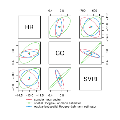
Figure 2: The left panel gives the scatter plot of the differences before and after the tilt for the corresponding variables of the LASERI data. The right panel shows the three estimated locations together with their confidence ellipsoids.

To illustrate the spatial signed-rank tests we consider the LASERI data which is publicly available in the R package ICSNP (Nordhausen et al., 2018). For that study several hemodynamic variables were monitored for 233 healthy subjects who were exposed to a passive head-up tilt, i.e. the subjects were first in a lying position, then tilted up before returning again to the lying position. One question here is whether, after the tilt back down and a resting period of 5 minutes, the hemodynamic variables returned to their pre-tilt levels. We will consider the three variables, heart rate (HR), cardiac output (CO), and average systemic vascular resistance index (SVRI), and look at the difference between the average value of the 5th minute before the tilt and the 5th minute after returning to the supine position. The null hypothesis is then that there is no difference, i.e., the location of the difference is $(0,0,0)^{\top}$. Using the R package MNM (Nordhausen & Oja, 2011), we computed for the data the location estimates with confidence ellipsoids as well as the asymptotic test for the transformation-retransformation and non-affine equivariant spatial HL-estimator and as a reference also the mean vector together with Hotelling’s $T^{2}$ test. Figure 2 shows in the left panel the scatter plot of the differences and on the right side the different location estimates with their confidence ellipsoids. The three location estimates are not that different, however, the non-affine equivariant HL-estimator has rather different confidence ellipsoids suffering from the fact that the scales of the three variables are very diverse. Comparing all ellipsoids indicates that the affine equivariant HL-estimator is the preferred choice for this data reflecting best the shape of the data and having the smallest volume. However, as for none of the estimates the ellipsoids contain $(0,0,0)^{\top}$ it comes as no surprise that all three tests yield p-values $<0.0001$.

6 High-dimensional case

So far the theory above is developed when the dimension $p$ of the distribution is fixed as is usually the case in classical multivariate statistics. In many modern applications however the dimension of the distributions is rather huge leading to a new asymptotic framework known as the high-dimensional regime. In such a high-dimensional framework the asymptotic behavior of the sample spatial median was recently studied in Zou et al. (2014) assuming spherical symmetry of an underlying distribution, where an asymptotic expansion of the spatial median was obtained and further applied to a sign-based test for the sphericity. Cheng et al. (2019) and Li & Xu (2022) studied the asymptotic behavior of the sample spatial median under the assumption of elliptical symmetry. Refining the asymptotic representation of the spatial median proposed in Cheng et al. (2019), Li & Xu (2022) gave a modified approximation of the spatial median, where the improvement is in that the Euclidean norm of the error term reduces to $o_{{\mathbb{P}}}(n^{-1/2})$. Such approximation enabled Li & Xu (2022) to establish a central limit theorem for the Euclidean distance of the sample spatial median to the population counterpart, further allowing for the development of one- and two-sample tests for high-dimensional mean vectors based on sample spatial medians. Motivated by the recent developments discussed above, in this section we consider an asymptotic representation of the spatial Hodges-Lehmann estimator in the high dimensional regime and under the assumption of sphericity. In the following, we adopt the notation

$$\textbf{u}_{i,j}=\textbf{z}_{i,j}/\|\textbf{z}_{i,j}\|,\quad{r}_{i,j}=\|\textbf{z}_{i,j}\|,\quad c_{k}=\mathbb{E}(r_{1,2}^{-k}),\,k\geq 1.$$

Assumption 3(a) we impose further in this section is comparable to those of Cheng et al. (2019), while Assumption 3(b) is a mild technical assumption ensuring that, in the limit, distribution of $\textbf{z}_{1,2}$ is not fully degenerate, in the sense that the rank of the corresponding covariance is uniformly larger than $1$.

Assumption 3

(a) $\limsup_{p}\mathbb{E}(r_{1,2}^{-4})<\infty$ and, for $1\leq k\leq 4$, $\limsup_{p}\mathbb{E}(r_{1,2}^{-k})/\mathbb{E}(r_{1,2}^{-1})^{k}=d_{k}<\infty$. (b) Leading eigenvalue $\lambda_{\mathrm{max}}(\mathrm{Cov}(\textbf{u}_{1,2}))$ of $\mathrm{Cov}(\textbf{u}_{1,2})$ is uniformly smaller than $1$, i.e. $\limsup_{p}\lambda_{\mathrm{max}}(\mathrm{Cov}(\textbf{u}_{1,2}))<1$.

Prior to stating the main result, we show that, for general underlying distribution satisfying Assumption 3, scaled sample Hodges-Lehman estimator ${\color[rgb]{0,0,0}{{\hat{\boldsymbol{\mu}}_{\mathrm{HL}}}}}$ is bounded in probability.

Theorem 9

Let $\textbf{y}_{1}\dots,\textbf{y}_{n}$ be a sample from $p$-variate distribution with $\mathbb{E}(\textbf{u}_{1,2})=\mathbf{0}$, and let $n,p\to\infty$. Then, under Assumption 3, $\sqrt{n}\ a_{p}{\color[rgb]{0,0,0}{{\hat{\boldsymbol{\mu}}_{\mathrm{HL}}}}}=O_{{\mathbb{P}}}(1)$, with choice of $a_{p}=\mathbb{E}(r_{1,2}^{-1})$.

Assume now that $\mathbf{y}_{1},\dots,\mathbf{y}_{n}$ is a random sample from an elliptical distribution $\mathcal{E}(\boldsymbol{\mu},2\boldsymbol{\Sigma})$ with mean ${\boldsymbol{\mu}}=\textbf{0}$ and covariance matrix $2\boldsymbol{\Sigma}\propto\textbf{I}_{p}$. Walsh averages $\textbf{z}_{i,j}=(\mathbf{y}_{i}+\mathbf{y}_{j})/2$, $i,j=1\dots,n$ then also follow the spherical distribution with location $\boldsymbol{\mu}$ and covariance matrix $\boldsymbol{\Sigma}$, thus admitting representation $\mathbf{z}_{i,j}=r_{i,j}\textbf{u}_{i,j}$, where $\textbf{u}_{i,j}$ is a random direction distributed uniformly on a unit sphere and independent of $r_{i,j}$. Using this notation it follows that $\boldsymbol{\Sigma}=p^{-1}\mathbb{E}(r_{1,2}^{2})\textbf{I}_{p}$. Note that Assumption 3 (b) is satisfied for the class of spherical distributions.

Theorem 10

Let $\textbf{y}_{1}\dots,\textbf{y}_{n}$ be a sample from $p$-variate symmetric distribution around the origin, and let $n,p\to\infty$. Then, under Assumption 3, for the sample Hodges-Lehman estimator ${\color[rgb]{0,0,0}{{\hat{\boldsymbol{\mu}}_{\mathrm{HL}}}}}$, $a_{p}\sqrt{n}\ {\color[rgb]{0,0,0}{{\hat{\boldsymbol{\mu}}_{\mathrm{HL}}}}}$ admits the following asymptotic representation:

$$a_{p}\sqrt{n}\ {\color[rgb]{0,0,0}{{\hat{\boldsymbol{\mu}}_{\mathrm{HL}}}}}=\sqrt{n}\binom{n}{2}^{-1}\sum_{i<j}\textbf{u}_{i,j}+o_{{\mathbb{P}}}(1),$$

with choice of $a_{p}=\mathbb{E}(r_{1,2}^{-1})$.

Theorem 10 can be a starting point for developing one- and two-sample tests for the high-dimensional mean which is, however, beyond the scope of this paper. To illustrate Theorem  10 however we performed a small simulation study to demonstrate that $\boldsymbol{\Delta}=\sqrt{n}\left(\binom{n}{2}^{-1}\sum_{i<j}r_{i,j}^{-1}\right){\color[rgb]{0,0,0}{{\hat{\boldsymbol{\mu}}_{\mathrm{HL}}}}}-\sqrt{n}\binom{n}{2}^{-1}\sum_{i<j}\textbf{u}_{i,j}$ decreases when $n$ and $p$ grow. Note that as $a_{p}$ is unknown, in the calculation of $\boldsymbol{\Delta}$, we estimate it using its consistent estimator $\binom{n}{2}^{-1}\sum_{i<j}r_{i,j}^{-1}$; see the latter part of proof of Theorem 10 for more insight.

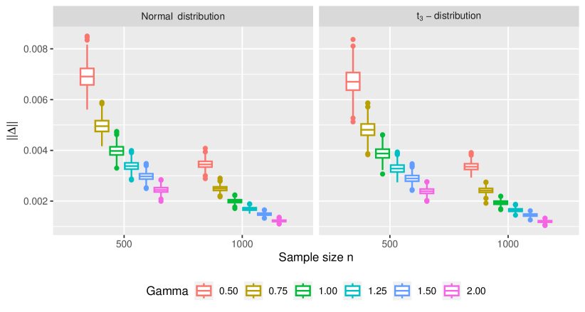
Figure 3: Boxplots of $||\boldsymbol{\Delta}||$ based on 1000 repetitions for different sample sizes $n$ and $\gamma=p/n$ values.

Based on 1000 repetitions Figure 3 shows $||\boldsymbol{\Delta}||$ for different sample sizes $n$ and $\gamma=p/n$’s when $\mathbf{y}$ either follows a $p$-variate standard normal distribution or a $p$-variate $t_{3}$ distribution with $\boldsymbol{\Sigma}=\mathbf{I}_{p}$, and illustrates the limiting behaviour of $\|\boldsymbol{\Delta}\|$, in the high-dimensional regime (Assumption 3). More precisely, as $n$ and $p$ increase, the approximation from Theorem 10 becomes more accurate, i.e. $\|\boldsymbol{\Delta}\|$ decreases, where already for $n=500$ and $p=250$, the median norm of the approximation error is below $0.007$.

7 Conclusion

The univariate HL-estimator has a long successful tradition as a location estimator. In this contribution we presented asymptotic results for a multivariate extension based on the concept of spatial signed-ranks yielding the spatial HL-estimator and the transformation-retransformation spatial HL-estimator in the classical multivariate framework where several of the statements appeared earlier in the literature, however often without proofs. What is also novel in this contribution is a first consideration of the spatial HL-estimator in a high-dimensional framework which can be a stepping stone to develop corresponding tests and considerations in the multisample case. Note that in the high-dimensional regime, affine equivariance is not a meaningful concept, and thus we work solely under the framework of orthogonal equivariance. Similarly, recall that under symmetry all the location estimators discussed will estimate the symmetry center while otherwise they are estimating different population quantities.

Appendix A: Proofs and auxiliary results

Lemma A.1

Let $\textbf{y}_{1},\dots,\textbf{y}_{n}$ be iid random vectors. Let $f(\|(\textbf{y}_{i}+\textbf{y}_{j})/2\|)$ be a function for which $\mathrm{Var}(f(\|(\textbf{y}_{i}+\textbf{y}_{j})/2\|))<\infty$. Then,

$${\binom{n}{2}}^{-1}\sum_{i<j}f(\|(\textbf{y}_{i}+\textbf{y}_{j})/2\|)\stackrel{{\scriptstyle a.s.}}{{\longrightarrow}}\mathbb{E}(f(\|(\textbf{y}_{1}+\textbf{y}_{2})/2\|)).$$

Proof of Lemma A.1

See for example Lee (1990). $\square$

Note that if we define

$$f(\|(\textbf{y}_{i}+\textbf{y}_{j})/2\|)=\left\|\frac{\textbf{y}_{i}+\textbf{y}_{j}}{2}-\boldsymbol{\mu}\right\|-\left\|\frac{\textbf{y}_{i}+\textbf{y}_{j}}{2}\right\|$$

Lemma A.1 implies that $d_{2n}(\boldsymbol{\mu})\stackrel{{\scriptstyle a.s.}}{{\longrightarrow}}d_{2}(\boldsymbol{\mu})$ for all $\boldsymbol{\mu}$.

The following key result for convex processes can be found in Lemma 2.2 in Davis et al. (1992) and Theorem 1 in Arcones (1998).

Lemma A.2

Let $g_{n}(\boldsymbol{\theta})$, $\boldsymbol{\theta}\in\mathbb{R}^{p}$, be a sequence of convex stochastic processes, and let $g(\boldsymbol{\theta})$ be a convex (limit) process, meaning that the finite dimensional distributions of $g_{n}(\boldsymbol{\theta})$ converge to those of $g(\boldsymbol{\theta})$. Let further $\hat{\boldsymbol{\theta}},\,\hat{\boldsymbol{\theta}}_{1},\dots,\hat{\boldsymbol{\theta}}_{n}$ be a sequence of random vectors satisfying

$$g(\hat{\boldsymbol{\theta}})=\inf_{\boldsymbol{\theta}}g(\boldsymbol{\theta}),\quad g_{n}(\hat{\boldsymbol{\theta}}_{n})=\inf_{\boldsymbol{\theta}}g_{n}(\boldsymbol{\theta}),\quad n=1,2,\dots.$$

If $\hat{\boldsymbol{\theta}}$ is unique with probability 1 then $\hat{\boldsymbol{\theta}}_{n}\stackrel{{\scriptstyle d}}{{\longrightarrow}}\hat{\boldsymbol{\theta}}$.

The following lemma is the result of the Lemma 19 of Arcones (1998). See also Bai et al. (1990) and Oja (2010).

Lemma A.3

The accuracies of constant, linear and quadratic approximations of the function $\boldsymbol{\mu}\mapsto\|\mathbf{z}-\boldsymbol{\mu}\|$ can be given by
(A1) $|\|\mathbf{z}-\boldsymbol{\mu}\|-\|\mathbf{z}\||\leq\|\boldsymbol{\mu}\|,$ (A2) $|\|\mathbf{z}-\boldsymbol{\mu}\|-\|\mathbf{z}\|+\mathbf{u}^{\top}\boldsymbol{\mu}|\leq 2r^{-1}\|\boldsymbol{\mu}\|^{2},$ (A3) $|\|\mathbf{z}-\boldsymbol{\mu}\|-\|\mathbf{z}\|+\mathbf{u}^{\top}\boldsymbol{\mu}-\boldsymbol{\mu}^{\top}(2r)^{-1}[\mathbf{I}_{p}-\mathbf{u}\mathbf{u}^{\top}]\boldsymbol{\mu}|\leq cr^{-1-\delta}\|\boldsymbol{\mu}\|^{2+\delta}$ for all $0<\delta<1$,
where $\mathbf{z}=r\mathbf{u}$, $r=\|\mathbf{z}\|$, $\mathbf{u}=\|\mathbf{z}\|^{-1}\mathbf{z}$ and the constant $c$ does not depend on $\mathbf{z}$ or $\boldsymbol{\mu}$.

Proof of Lemma A.3

See e.g. Oja (2010). $\square$

Proof of Theorem 5

As $d_{2n}(\boldsymbol{\mu})$ and $d_{2}(\boldsymbol{\mu})$ are bounded and convex, also $\sup_{\|\boldsymbol{\mu}\|\leq C}|d_{2n}(\boldsymbol{\mu})-d_{2}(\boldsymbol{\mu})|\stackrel{{\scriptstyle a.s.}}{{\longrightarrow}}0$, for all $C>0$ (Theorem 10.8 in Rockafellar (1970)). Write $\hat{\boldsymbol{\mu}}_{\mathrm{HL}}^{*}=\operatorname*{argmin}_{\|\boldsymbol{\mu}\|\leq C}d_{2n}(\boldsymbol{\mu})$. Then $d_{2}(\hat{\boldsymbol{\mu}}_{\mathrm{HL}}^{*})\to 0$ and $\hat{\boldsymbol{\mu}}_{\mathrm{HL}}^{*}\to\mathbf{0}$ almost surely as $d_{2}(\mathbf{0})=0$, $|d_{2n}({\hat{\boldsymbol{\mu}}_{\mathrm{HL}}}^{*})-d_{2}({\hat{\boldsymbol{\mu}}_{\mathrm{HL}}}^{*})|\stackrel{{\scriptstyle a.s.}}{{\longrightarrow}}0$, and $d_{2n}({\hat{\boldsymbol{\mu}}_{\mathrm{HL}}}^{*})\leq d_{2n}(\mathbf{0})\stackrel{{\scriptstyle a.s.}}{{\longrightarrow}}d_{2}(\mathbf{0})\leq d_{2}({\hat{\boldsymbol{\mu}}_{\mathrm{HL}}}^{*}).$ The result then follows as, using any $C^{\prime}>C$, the sequence of estimators $\operatorname*{argmin}_{\|\boldsymbol{\mu}\|\leq C^{\prime}}d_{2n}(\boldsymbol{\mu})$ and $\hat{\boldsymbol{\mu}}_{\mathrm{HL}}^{*}$ are the same almost surely (use again Theorem 10.8 in Rockafellar (1970)). $\square$

Proof of Theorem 6

Define the sample statistic

$$\hat{\mathbf{A}}={\binom{n}{2}}^{-1}\sum_{i<j}\|\mathbf{z}_{i,j}\|^{-1}(\mathbf{I}_{p}-\|\mathbf{z}_{i,j}\|^{-2}\mathbf{z}_{i,j}\mathbf{z}_{i,j}^{\top})$$

and the corresponding population value

$$\mathbf{A}=\mathbb{E}(\hat{\mathbf{A}})=\mathbb{E}\{\|\mathbf{z}_{i,j}\|^{-1}(\mathbf{I}_{p}-\|\mathbf{z}_{i,j}\|^{-2}\mathbf{z}_{i,j}\mathbf{z}_{i,j}^{\top})\}.$$

Note that $\|\mathbf{z}\|^{-1}(\mathbf{I}_{p}-\|\mathbf{z}\|^{-2}\mathbf{z}\mathbf{z}^{\top})$ is the Hessian matrix of $\|\mathbf{z}-\boldsymbol{\mu}\|$ evaluated at $\boldsymbol{\mu}=\mathbf{0}$.

The approximation (A3) of the Lemma A.3 implies that

$$\left|\sum_{i<j}\left\{\|\mathbf{z}_{i,j}-\boldsymbol{\mu}\|-\|\mathbf{z}_{i,j}\|+\mathbf{u}_{i,j}^{\top}\boldsymbol{\mu}-\boldsymbol{\mu}^{\top}(2r_{i,j})^{-1}[\mathbf{I}_{p}-\mathbf{u}_{i,j}\mathbf{u}_{i,j}^{\top}]\boldsymbol{\mu}\right\}\right|\leq c\|\boldsymbol{\mu}\|^{2+\delta}\sum_{i<j}\frac{1}{r_{i,j}^{1+\delta}}$$

Replacing $\boldsymbol{\mu}$ by $n^{-1/2}\boldsymbol{\mu}$ and multiplying both sides of the inequality by the constant $n{\binom{n}{2}}^{-1}$ gives the approximation

$$\bigg{|}n{\binom{n}{2}}^{-1}\sum_{i<j}\left\{\|\mathbf{z}_{i,j}-n^{-1/2}\boldsymbol{\mu}\|-\|\mathbf{z}_{i,j}\|\right\}+n^{1/2}{\binom{n}{2}}^{-1}\sum_{i<j}\frac{\mathbf{z}_{i,j}^{\top}}{\|\mathbf{z}_{i,j}\|}\boldsymbol{\mu}$$

$$-\boldsymbol{\mu}^{\top}{\binom{n}{2}}^{-1}\sum_{i<j}\left[\frac{1}{2\|\mathbf{z}_{i,j}\|}\left[\mathbf{I}_{p}-\frac{\mathbf{z}_{i,j}\mathbf{z}_{i,j}^{\top}}{\|\mathbf{z}_{i,j}\|^{2}}\right]\right]\boldsymbol{\mu}\bigg{|}$$

$$=\left|nd_{2n}(n^{-1/2}\boldsymbol{\mu})+(\sqrt{n}\mathbf{q}_{n})^{\top}\boldsymbol{\mu}-\frac{1}{2}\boldsymbol{\mu}^{\top}\hat{\mathbf{A}}\boldsymbol{\mu}\right|\leq n{\binom{n}{2}}^{-1}\frac{c\|\boldsymbol{\mu}\|^{2+\delta}}{n^{(2+\delta)/2}}\sum_{i<j}\frac{1}{r_{i,j}^{1+\delta}},$$

where (see Lee (1990)) $\hat{\mathbf{A}}\stackrel{{\scriptstyle a.s.}}{{\longrightarrow}}\mathbf{A}$ and

$$\sqrt{n}\mathbf{q}_{n}=\sqrt{n}\left[\left\{{\binom{n}{2}}^{-1}\sum_{i<j}\frac{\mathbf{z}_{i,j}}{\|\mathbf{z}_{i,j}\|}\right\}-\mathbf{0}\right]\stackrel{{\scriptstyle d}}{{\longrightarrow}}N_{p}(\mathbf{0},4\mathbf{B}),$$

where $\mathbf{B}=E\{(\|\mathbf{z}_{1,2}\|^{-1}\mathbf{z}_{1,2})(\|\mathbf{z}_{2,3}\|^{-1}\mathbf{z}_{2,3}^{\top})\}.$ We now get under Assumption 2 that

$$n~{}d_{2n}(n^{-1/2}\boldsymbol{\mu})-\left(-(\sqrt{n}~{}\mathbf{q}_{n})^{\top}\boldsymbol{\mu}+\frac{1}{2}\boldsymbol{\mu}^{\top}\mathbf{A}\boldsymbol{\mu}\right)\stackrel{{\scriptstyle{\mathbb{P}}}}{{\longrightarrow}}0.$$

We can then apply Lemma A.2 with $g_{n}(\boldsymbol{\mu})=n~{}d_{2n}(n^{-1/2}\boldsymbol{\mu})$ and $g(\boldsymbol{\mu})=-\mathbf{h}^{\top}\boldsymbol{\mu}+\frac{1}{2}\boldsymbol{\mu}^{\top}\mathbf{A}\boldsymbol{\mu},$ where $\mathbf{h}\sim N_{p}(\mathbf{0},4\mathbf{B})$. Next, taking the gradient of $-(\sqrt{n}~{}\mathbf{q}_{n})^{\top}\boldsymbol{\mu}+\frac{1}{2}\boldsymbol{\mu}^{\top}\mathbf{A}\boldsymbol{\mu}$ with respect to $\boldsymbol{\mu}$ and setting it to zero gives ($\mathbf{A}$ is nonsingular)

$$\sqrt{n}{\color[rgb]{0,0,0}{{\hat{\boldsymbol{\mu}}_{\mathrm{HL}}}}}\stackrel{{\scriptstyle d}}{{\longrightarrow}}N_{p}(\mathbf{0},4\mathbf{A}^{-1}\mathbf{B}\mathbf{A}^{-1}).$$

$\square$

Lemma A.4

Let $\mathbf{Y}=(\mathbf{y}_{1},\ldots,\mathbf{y}_{n})^{\top}$ be a random sample from a symmetric distribution satisfying Assumption 1. Assume also that scatter matrix $\mathbf{S}=\mathbf{S}(\mathbf{Y})$ satisfies $\sqrt{n}(\mathbf{S}^{-1/2}-\mathbf{I}_{p})=O_{{\mathbb{P}}}(1)$. Then

$$\sqrt{n}({\mathbf{q}}_{n}(\mathbf{Y}^{*})-{\mathbf{q}}_{n}(\mathbf{Y}))\stackrel{{\scriptstyle{\mathbb{P}}}}{{\longrightarrow}}\mathbf{0},$$

where

$${\mathbf{q}}_{n}(\mathbf{Y})={\binom{n}{2}}^{-1}\sum_{i<j}\mathbf{u}((\mathbf{y}_{i}+\mathbf{y}_{j})/2)={\binom{n}{2}}^{-1}\sum_{i<j}\mathbf{u}(\mathbf{z}_{i,j}).$$

Proof of Lemma A.4

Let $\boldsymbol{\Delta}_{n}=\sqrt{n}(\mathbf{S}^{-1/2}-\mathbf{I}_{p})$. Then ${\mathbf{S}}^{-1/2}=\mathbf{I}_{p}+n^{-1/2}\boldsymbol{\Delta}_{n},$ where $\boldsymbol{\Delta}_{n}$ is bounded in probability. Using the approximation (B2) in Möttönen et al. (2010) we obtain

$$\sqrt{n}{\binom{n}{2}}^{-1}\sum_{i<j}\mathbf{u}(\mathbf{S}^{-1/2}\mathbf{z}_{i,j})-\sqrt{n}{\binom{n}{2}}^{-1}\sum_{i<j}\mathbf{u}(\mathbf{z}_{i,j})=-{\binom{n}{2}}^{-1}\sum_{i<j}\mathbf{g}(\mathbf{z}_{i,j})+o_{{\mathbb{P}}}(1),$$

where $\mathbf{g}(\mathbf{z}_{i,j})=[\mathbf{I}_{p}-\mathbf{u}(\mathbf{z}_{i,j})\mathbf{u}(\mathbf{z}_{i,j})^{\top}]\boldsymbol{\Delta}_{n}\mathbf{u}(\mathbf{z}_{i,j})$ is symmetrically distributed around the origin as multiplying all the observation by $-1$ simply changes its sign only. Let $|\boldsymbol{\Delta}_{n}|$ denote the Frobenius norm $(\mbox{tr}(\boldsymbol{\Delta}_{n}^{\top}\boldsymbol{\Delta}_{n}))^{1/2}$. Then ${\binom{n}{2}}^{-1}\sum_{i<j}\mathbf{g}(\mathbf{z}_{i,j})1_{|\boldsymbol{\Delta}_{n}|\leq M}$ converges in probability to zero for all $M>0$. As ${\mathbb{P}}(|\boldsymbol{\Delta}_{n}|>M)$ can be made arbitrarily close to zero,

$$\sqrt{n}{\binom{n}{2}}^{-1}\sum_{i<j}\mathbf{u}(\mathbf{S}^{-1/2}\mathbf{z}_{i,j})-\sqrt{n}{\binom{n}{2}}^{-1}\sum_{i<j}\mathbf{u}(\mathbf{z}_{i,j})\stackrel{{\scriptstyle{\mathbb{P}}}}{{\longrightarrow}}0$$

and the proof follows. $\square$

Lemma A.5

Let $\mathbf{Y}=(\mathbf{y}_{1},\ldots,\mathbf{y}_{n})^{\top}$ be a random sample from a distribution satisfying Assumption 1. Assume also that scatter matrix $\mathbf{S}=\mathbf{S}(\mathbf{Y})$ satisfies $\sqrt{n}(\mathbf{S}-\mathbf{I}_{p})=O_{{\mathbb{P}}}(1)$. Let $\mathbf{Y}^{*}=\mathbf{Y}({\mathbf{S}}^{-1/2})^{\top}$. Then

$$\mathbf{A}(\mathbf{Y}^{*})-\mathbf{A}(\mathbf{Y})\stackrel{{\scriptstyle{\mathbb{P}}}}{{\longrightarrow}}\mathbf{0}\ \ \mbox{and}\ \ \mathbf{B}(\mathbf{Y}^{*})-\mathbf{B}(\mathbf{Y})\stackrel{{\scriptstyle{\mathbb{P}}}}{{\longrightarrow}}\mathbf{0}.$$

Proof of Theorem 7

Let ${\mathbf{S}}^{-1/2}=\mathbf{I}_{p}+n^{-1/2}\boldsymbol{\Delta}_{n}$ and ${\mathbf{z}}_{i,j}^{*}=(\mathbf{I}_{p}+n^{-1/2}\boldsymbol{\Delta}_{n})\mathbf{z}_{i,j}$, $i,j=1,\ldots,n$.

The approximation (A3) of the Lemma A.3 gives the result

$$\bigg{|}n{\binom{n}{2}}^{-1}\sum_{i<j}\left\{\|\mathbf{z}_{i,j}^{*}-n^{-1/2}\boldsymbol{\mu}\|-\|\mathbf{z}_{i,j}^{*}\|\right\}+\sqrt{n}{\binom{n}{2}}^{-1}\sum_{i<j}\frac{\mathbf{z}_{i,j}^{*\top}}{\|\mathbf{z}_{i,j}^{*}\|}\boldsymbol{\mu}$$

$$-\boldsymbol{\mu}^{\top}\bigg{\{}{\binom{n}{2}}^{-1}\sum_{i<j}\frac{1}{2\|\mathbf{z}_{i,j}^{*}\|}\bigg{[}\mathbf{I}_{p}-\frac{\mathbf{z}_{i,j}^{*}\mathbf{z}_{i,j}^{*\top}}{\|\mathbf{z}_{i,j}^{*}\|^{2}}\bigg{]}\bigg{\}}\boldsymbol{\mu}\bigg{|}$$

$$\leq\frac{c\|\boldsymbol{\mu}\|^{2+\delta}}{n^{\delta/2}}{\binom{n}{2}}^{-1}\sum_{i<j}\|(\mathbf{I}_{p}+n^{-1/2}\boldsymbol{\Delta}_{n})\mathbf{z}_{i,j}\|^{-1-\delta}\stackrel{{\scriptstyle{\mathbb{P}}}}{{\longrightarrow}}0.$$

Lemmas A.2, A.4 and A.5 imply that $\sqrt{n}\ {\color[rgb]{0,0,0}{{\hat{\boldsymbol{\mu}}_{\mathrm{HL}}}}}(\mathbf{Y}^{*})$ and $\sqrt{n}\ {\color[rgb]{0,0,0}{{\hat{\boldsymbol{\mu}}_{\mathrm{HL}}}}}(\mathbf{Y})$ have the same limiting distribution. The result then follows from Slutsky’s theorem. $\square$

Proof of Theorem 9

The HL median is a spatial median of the sample $\textbf{z}_{i,j}$, $i,j=1,\dots,n$ and thus minimizes the objective function ${\color[rgb]{0,0,0}{{d_{2n}}}}(\boldsymbol{\mu})=\binom{n}{2}^{-1}\sum_{i<j}\|\textbf{z}_{i,j}-\boldsymbol{\mu}\|-\sum_{i<j}\|\textbf{z}_{i,j}\|$. Write now $a_{p}\sqrt{n}\boldsymbol{\mu}=C\textbf{v}$, where $C>0$ and $\|\textbf{v}\|=1$. The aim is now to show that for $\varepsilon>0$ there exists $C>0$ such that

$$\liminf_{n}\mathbb{P}\left(\inf_{\textbf{v}}{\color[rgb]{0,0,0}{{d_{2n}}}}(Ca_{p}^{-1}n^{-1/2}\textbf{v})>0\right)>1-\varepsilon.$$

Convexity of ${\color[rgb]{0,0,0}{{d_{2n}}}}$ then implies that also $\mathbb{P}(\|a_{p}\sqrt{n}\ {\color[rgb]{0,0,0}{{\hat{\boldsymbol{\mu}}_{\mathrm{HL}}}}}\|\leq C)>1-\varepsilon$, i.e ${\color[rgb]{0,0,0}{{\hat{\boldsymbol{\mu}}_{\mathrm{HL}}}}}=O_{{\mathbb{P}}}(a_{p}^{-1}n^{-1/2})$. The approximation (A3) in Möttönen et al. (2010) gives that for every $\delta\in(0,1)$

$$\frac{a_{p}\sqrt{n}}{C}{\color[rgb]{0,0,0}{{d_{2n}}}}\left(\frac{C}{a_{p}\sqrt{n}}\mathbf{v}\right)\geq-\sqrt{n}U_{1}+CU_{2}-C_{1}(C^{1+\delta}/n^{\delta/2})U_{3}$$

where $U_{1}={\binom{n}{2}}^{-1}\sum_{i<j}\textbf{u}_{i,j}^{\top}\textbf{v},\ \ U_{2}={\binom{n}{2}}^{-1}\sum_{i<j}\frac{1}{2(a_{p}r_{i,j})}\{1-(\textbf{v}^{\top}\textbf{u}_{i,j})^{2}\}$, $U_{3}={\binom{n}{2}}^{-1}\sum_{i<j}\frac{1}{(a_{p}r_{i,j})^{1+\delta}},$ and $C_{1}$ is a universal constant (not depending on $n,p$ or $\delta$). The random variables $U_{1}$, $U_{2}$ and $U_{3}$ are all univariate U-statistics with a well-developed theory. As $\mathbb{E}(r_{i,j}^{-k})<\infty$ for $k\leq 4$, these U-statistics have finite expectation and variances. Further

$$CU_{2}-C_{1}(C^{1+\delta}/n^{\delta/2})U_{3}=C\mathbb{E}[U_{2}]-C_{1}(C^{1+\delta}/n^{\delta/2})\mathbb{E}[U_{3}]+U$$

where $U$ is a U-statistic with the mean zero, finite variance, and $\sqrt{n}U=O_{{\mathbb{P}}}(1)$. The lower bound can be written as

$$\frac{a_{p}\sqrt{n}}{C}{\color[rgb]{0,0,0}{{d_{2n}}}}(Ca_{p}^{-1}n^{-1/2}\textbf{v})\geq-\sqrt{n}U_{1}+C\mathbb{E}[U_{2}]-C_{1}(C^{1+\delta}/n^{\delta/2})\mathbb{E}[U_{3}]+o_{{\mathbb{P}}}(1).$$

Assumption 3 (a) ensures that $\mathbb{E}(1-(\textbf{v}^{\top}\textbf{u}_{1,2})^{2})\geq C_{2}$, for some universal constant $C_{2}>0$, further giving $\mathbb{E}(U_{2})\geq{C_{2}}/{2}$. On the other hand, Assumption 3 (b) gives that $\mathbb{E}(U_{3})=O(1)$. We thus obtain the lower bound

$$\frac{a_{p}\sqrt{n}}{C}{\color[rgb]{0,0,0}{{d_{2n}}}}(Ca_{p}^{-1}n^{-1/2}\textbf{v})\geq-\sqrt{n}U_{1}+\frac{{\color[rgb]{0,0,0}{{C_{2}}}}}{2}C+o_{{\mathbb{P}}}(1).$$

As $\mathrm{tr}(\mathbb{E}(\textbf{u}_{1,2}\textbf{u}_{1,2}^{\top}))=1$, the eigenvalues of the covariance of $\textbf{u}_{1,2}$ are uniformly bounded from above by $1$. Thus, $\sqrt{n}U_{1}={\color[rgb]{0,0,0}{{O_{p}(1)}}}$ further implying that for every $\varepsilon>0$, we can find $C>0$, so that for $n>0$ large enough

$${\mathbb{P}}\{{\color[rgb]{0,0,0}{{-\sqrt{n}U_{1}+{{C_{2}}}C/2+o_{{\mathbb{P}}}(1)}}}>0\}>1-\epsilon,$$

thus completing the proof. $\square$

Proof of Theorem 10

The approximation (B2) in Möttönen et al. (2010) gives that for $\boldsymbol{\mu}={\color[rgb]{0,0,0}{{\hat{\boldsymbol{\mu}}_{\mathrm{HL}}}}}\in\mathbb{R}^{p}$ and $\delta\in(0,1)$

$$\binom{n}{2}^{-1}\sum_{i<j}\frac{\textbf{z}_{i,j}-\boldsymbol{\mu}}{\|\textbf{z}_{i,j}-\boldsymbol{\mu}\|}=\binom{n}{2}^{-1}\sum_{i<j}\left(\textbf{u}_{i,j}{\color[rgb]{0,0,0}{{-}}}r_{i,j}^{-1}(\textbf{I}_{p}-\textbf{u}_{i,j}\textbf{u}_{i,j}^{\top})\boldsymbol{\mu}\right)+\textbf{R}(\boldsymbol{\mu}),$$ (1)

where the norm of the remainder $\|\textbf{R}(\boldsymbol{\mu})\|\leq C\|\boldsymbol{\mu}\|^{1+\delta}\binom{n}{2}^{-1}\sum_{i<j}r_{i,j}^{-(1+\delta)}$, for some universal constant $C>0$ (does not depend on $n,\,p$). Observing that $\displaystyle\binom{n}{2}^{-1}\sum_{i<j}\frac{\textbf{z}_{i,j}-{\color[rgb]{0,0,0}{{\hat{\boldsymbol{\mu}}_{\mathrm{HL}}}}}}{\|\textbf{z}_{i,j}-{\color[rgb]{0,0,0}{{\hat{\boldsymbol{\mu}}_{\mathrm{HL}}}}}\|}={\color[rgb]{0,0,0}{{\mathbf{0}}}}$ and substituting ${\color[rgb]{0,0,0}{{\hat{\boldsymbol{\mu}}_{\mathrm{HL}}}}}=n^{-1/2}a_{p}^{-1}{\hat{\boldsymbol{\mu}}_{\mathrm{HL}}}^{*}$ in (1), we obtain

$$\sqrt{n}\textbf{T}-\textbf{A}{\hat{\boldsymbol{\mu}}_{\mathrm{HL}}}^{*}=\textbf{R}({\hat{\boldsymbol{\mu}}_{\mathrm{HL}}}^{*})$$

where

$$\textbf{T}={\binom{n}{2}}^{-1}\sum_{i<j}\textbf{u}_{i,j}\ \ \ \mbox{and}\ \ \ \textbf{A}={\binom{n}{2}}^{-1}\sum_{i<j}\left[\frac{1}{a_{p}r_{i,j}}(\textbf{I}-\textbf{u}_{i,j}\textbf{u}_{i,j}^{\top})\right]$$

and

$$\|\mathbf{R}({\hat{\boldsymbol{\mu}}_{\mathrm{HL}}}^{*})\|\leq C_{2}n^{-\delta/2}|{\hat{\boldsymbol{\mu}}_{\mathrm{HL}}}^{*}|^{1+\delta}\left[{\binom{n}{2}}^{-1}\sum_{i<j}(a_{p}r_{i,j})^{-(1+\delta)}\right]\stackrel{{\scriptstyle{\mathbb{P}}}}{{\longrightarrow}}0$$

Next show that $\mathbf{D}({\hat{\boldsymbol{\mu}}_{\mathrm{HL}}}^{*})={\binom{n}{2}}^{-1}\sum_{i<j}\left[\frac{1}{a_{p}r_{i,j}}\mathbf{u}_{i,j}\mathbf{u}_{i,j}^{\top}\right]{\hat{\boldsymbol{\mu}}_{\mathrm{HL}}}^{*}=o_{{\mathbb{P}}}(1)$. Write first ${\color[rgb]{0,0,0}{{\boldsymbol{\mu}=c\textbf{v}}}}$ where $0<c<C$ and $\mathbf{v}^{\prime}\mathbf{v}=1$. Then, under sphericity, $\mathbf{D}(\boldsymbol{\mu})$ is a U-statistics with expected value $(c/p)\mathbf{v}$ and (by triangular inequality)

$$\|\mathbf{D}({\color[rgb]{0,0,0}{{\boldsymbol{\mu}}}})\|\leq C{\binom{n}{2}}^{-1}\sum_{i<j}\left[\frac{1}{a_{p}r_{i,j}}|{\color[rgb]{0,0,0}{{\textbf{u}_{i,j}^{\top}\textbf{v}}}}|\right]$$

and the upper limit is a U-statistic with the expected value at most $C/\sqrt{p}$ and the variance $O(1/(pn))$. Therefore the upper limit converges in probability to zero as $p\to\infty$. Finally, as ${\hat{\boldsymbol{\mu}}_{\mathrm{HL}}}^{*}=O_{{\mathbb{P}}}(1)$, also $\mathbf{D}({\hat{\boldsymbol{\mu}}_{\mathrm{HL}}}^{*})\stackrel{{\scriptstyle{\mathbb{P}}}}{{\longrightarrow}}0$. This is seen as

$${\mathbb{P}}(\|\mathbf{D}({\hat{\boldsymbol{\mu}}_{\mathrm{HL}}}^{*})\|\leq\epsilon)\leq{\mathbb{P}}(\|{\hat{\boldsymbol{\mu}}_{\mathrm{HL}}}^{*}\|\leq C)\cdot{\mathbb{P}}(\|\mathbf{D}({\hat{\boldsymbol{\mu}}_{\mathrm{HL}}}^{*})\|\leq\epsilon\ |\ \|{\hat{\boldsymbol{\mu}}_{\mathrm{HL}}}^{*}\|\leq C)+{\mathbb{P}}(\|{\hat{\boldsymbol{\mu}}_{\mathrm{HL}}}^{*}\|>C)$$

This gives us the second approximation (under sphericity)

$$\sqrt{n}\ \mathbf{T}-\left[{\binom{n}{2}}^{-1}\sum_{i<j}\frac{1}{a_{p}r_{i,j}}\right]\hat{\boldsymbol{\mu}}_{HL}^{*}=o_{{\mathbb{P}}}(1)$$

Finally as $\displaystyle{\binom{n}{2}}^{-1}\sum_{i<j}(a_{p}r_{i,j})^{-1}=1+(1/\sqrt{n})O_{{\mathbb{P}}}(1)$, we have the third approximation for ${\hat{\boldsymbol{\mu}}_{\mathrm{HL}}}^{*}=a_{p}\ \sqrt{n}\ {\color[rgb]{0,0,0}{{\hat{\boldsymbol{\mu}}_{\mathrm{HL}}}}}$:

$${\hat{\boldsymbol{\mu}}_{\mathrm{HL}}}^{*}=\sqrt{n}{\color[rgb]{0,0,0}{{\textbf{T}}}}+o_{{\mathbb{P}}}(1).$$

$\square$

References

• Arcones (1998) Arcones, M. A. (1998). Asymptotic Theory for $M$-Estimators over a Convex Kernel. Econometric Theory, 14, 387–422.
• Bai et al. (1990) Bai, Z. D., Chen, X. R., Miao, B. Q., & Rao, C. R. (1990). Asymptotic Theory of Least Distances Estimate in Multivariate Linear Models. Statistics, 21, 503–519.
• Brown (1983) Brown, B. M. (1983). Statistical Uses of the Spatial Median. Journal of the Royal Statistical Society. Series B, 45, 25–30.
• Chakraborty et al. (1998) Chakraborty, B., Chaudhuri, P., & Oja, H. (1998). Operating Transformation Retransformation on Spatial Median and Angle Test. Statistica Sinica, 8, 767–784.
• Chaudhuri (1992) Chaudhuri, P. (1992). Multivariate Location Estimation Using Extension of $R$-Estimates Through $U$-Statistics Type Approach. The Annals of Statistics, 20, 897 – 916.
• Cheng et al. (2019) Cheng, G., Liu, B., Peng, L., Zhang, B., & Zheng, S. (2019). Testing the Equality of Two High-Dimensional Spatial Sign Covariance Matrices. Scandinavian Journal of Statistics, 46, 257–271.
• Davis et al. (1992) Davis, R. A., Knight, K., & Liu, J. (1992). M-Estimation for Autoregressions with Infinite Variance. Stochastic Processes and their Applications, 40, 145–180.
• Feng & Sun (2016) Feng, L., & Sun, F. (2016). Spatial-Sign Based High-Dimensional Location Test. Electronic Journal of Statistics, 10, 2420 – 2434.
• Feng et al. (2016) Feng, L., Zou, C., & Wang, Z. (2016). Multivariate-Sign-Based High-Dimensional Tests for the Two-Sample Location Problem. Journal of the American Statistical Association, 111, 721–735.
• Frahm (2009) Frahm, G. (2009). Asymptotic Distributions of Robust Shape Matrices and Scales. Journal of Multivariate Analysis, 100, 1329–1337.
• Fritz et al. (2012) Fritz, H., Filzmoser, P., & Croux, C. (2012). A Comparison of Algorithms for the Multivariate L1-Median. Computational Statistics, 27, 393–410.
• Gini & Galvani (1929) Gini, C., & Galvani, L. (1929). Di talune estensioni dei concetti di media ai caratteri qualitativi. Metron, 8, 3–209.
• Haldane (1948) Haldane, J. B. S. (1948). Note on the Median of a Multivariate Distribution. Biometrika, 35, 414–417.
• Hallin & Paindaveine (2002) Hallin, M., & Paindaveine, D. (2002). Optimal Tests for Multivariate Location Based on Interdirections and Pseudo-Mahalanobis Ranks. The Annals of Statistics, 30, 1103 – 1133.
• Hettmansperger et al. (1997) Hettmansperger, T. P., Möttönen, J., & Oja, H. (1997). Affine-Invariant Multivariate One-Sample Signed-Rank Tests. Journal of the American Statistical Association, 92, 1591–1600.
• Hettmansperger & Randles (2002) Hettmansperger, T. P., & Randles, R. H. (2002). A Practical Affine Equivariant Multivariate Median. Biometrika, 89, 851–860.
• Hodges & Lehmann (1963) Hodges, J. L., & Lehmann, E. L. (1963). Estimates of Location Based on Rank Tests. The Annals of Mathematical Statistics, 34, 598 – 611.
• Hoeffding (1948) Hoeffding, W. (1948). A Class of Statistics with Asymptotically Normal Distribution. The Annals of Mathematical Statistics, 19, 293–325.
• Hössjer & Croux (1995) Hössjer, O., & Croux, C. (1995). Generalizing Univariate Signed Rank Statistics for Testing and Estimating a Multivariate Location Parameter. Journal of Nonparametric Statistics, 4, 293–308.
• Ilmonen et al. (2012) Ilmonen, P., Oja, H., & Serfling, R. (2012). On Invariant Coordinate System (ICS) Functionals. International Statistical Review, 80, 93–110.
• Kent et al. (2015) Kent, J. T., Er, F., & Constable, P. D. L. (2015). Algorithms for the Spatial Median. In K. Nordhausen, & S. Taskinen (Eds.) Modern Nonparametric, Robust and Multivariate Methods: Festschrift in Honour of Hannu Oja, (pp. 205–224). Cham: Springer.
• Lee (1990) Lee, A. J. (1990). $U$-Statistics: Theory and Practice. Routledge.
• Li & Xu (2022) Li, W., & Xu, Y. (2022). Asymptotic Properties of High-Dimensional Spatial Median in Elliptical Distributions with Application. Journal of Multivariate Analysis, 190, 104975.
• Magyar & Tyler (2011) Magyar, A., & Tyler, D. (2011). The Asymptotic Efficiency of the Spatial Median for Elliptically Symmetric Distributions. Sankhya B, 73, 165–192.
• Möttönen et al. (2010) Möttönen, J., Nordhausen, K., & Oja, H. (2010). Asymptotic Theory of the Spatial Median. In J. Antoch, M. Huskova, & P. Sen (Eds.) Nonparametrics and Robustness in Modern Statistical Inference and Time Series Analysis, vol. 7, (pp. 182–193). Institute of Mathematical Statistics.
• Möttönen & Oja (1995) Möttönen, J., & Oja, H. (1995). Multivariate Spatial Sign and Rank Methods. Journal of Nonparametric Statistics, 5, 201–213.
• Möttönen et al. (2005) Möttönen, J., Oja, H., & Serfling, R. J. (2005). Multivariate Generalized Spatial Signed-Rank Methods. Journal of Statistical Research, 39, 19 – 42.
• Nordhausen & Oja (2011) Nordhausen, K., & Oja, H. (2011). Multivariate $L_{1}$ Methods: The Package MNM. Journal of Statistical Software, 43, 1–28.
• Nordhausen et al. (2018) Nordhausen, K., Sirkiä, S., Oja, H., & Tyler, D. E. (2018). ICSNP: Tools for Multivariate Nonparametrics. R package version 1.1-1.
• Oja (2010) Oja, H. (2010). Multivariate Nonparametric Methods with R. An Approach Based on Spatial Signs and Ranks. Springer.
• Oja (2013) Oja, H. (2013). Multivariate Median. In C. Becker, R. Fried, & S. Kuhnt (Eds.) Robustness and Complex Data Structures: Festschrift in Honour of Ursula Gather, (pp. 3–15). Berlin: Springer.
• Puri & Sen (1971) Puri, M. L., & Sen, P. K. (1971). Nonparametric Methods in Multivariate Analysis. New York, USA: John Wiley & Sons.
• Randles (1989) Randles, R. H. (1989). A Distribution-Free Multivariate Sign Test Based on Interdirections. Journal of the American Statistical Association, 84, 1045–1050.
• Rockafellar (1970) Rockafellar, R. T. (1970). Convex Analysis. Princeton: Princeton University Press.
• Sen (1963) Sen, P. K. (1963). On the Estimation of Relative Potency in Dilution (-Direct) Assays by Distribution-Free Methods. Biometrics, 19, 532–552.
• Small (1990) Small, C. G. (1990). A Survey of Multidimensional Medians. International Statistical Review, 58, 263–277.
• Taskinen et al. (2023) Taskinen, S., Frahm, G., Nordhausen, K., & Oja, H. (2023). A Review of Tyler’s Shape Matrix and Its Extensions. In M. Yi, & K. Nordhausen (Eds.) Robust and Multivariate Statistical Methods: Festschrift in Honor of David E. Tyler, (pp. 23–41). Cham: Springer.
• Tyler (1987) Tyler, D. E. (1987). A Distribution-Free $M$-Estimator of Multivariate Scatter. The Annals of Statistics, 15, 234 – 251.
• Tyler et al. (2009) Tyler, D. E., Critchley, F., Dümbgen, L., & Oja, H. (2009). Invariant Coordinate Selection. Journal of the Royal Statistical Society. Series B, 71, 549–92.
• Vardi & Zhang (2000) Vardi, Y., & Zhang, C.-H. (2000). The Multivariate $L_{1}$-Median and Associated Data Depth. Proceedings of the National Academy of Sciences, 97, 1423–1426.
• Zou et al. (2014) Zou, C., Peng, L., Feng, L., & Wang, Z. (2014). Multivariate Sign-Based High-Dimensional Tests for Sphericity. Biometrika, 101, 229–236.