Holevo Cramér-Rao Bound for waveform estimation of gravitational waves

Abstract

Detecting kilohertz gravitational waves from the post-merger remnants of binary neutron-star mergers could enhance our understanding of extreme matter. To enable this detection, a gravitational-wave interferometer can be detuned to increase its kilohertz sensitivity. The precision limits of detuned interferometers and other cavity–based quantum sensors, however, are not well understood. The sensitivity of the standard variational readout scheme does not reach the waveform-estimation Quantum Cramér-Rao Bound. We establish the fundamental precision limit, the waveform-estimation Holevo Cramér-Rao Bound, by identifying the incompatibility of the naïve estimates of the signal’s cosine and sine phases. For an equal weighting between the phases, we prove that the standard scheme is indeed optimal. For unequal weights, however, we propose an experimental realisation of a new measurement scheme to significantly improve the sensitivity. This scheme could facilitate kilohertz gravitational-wave astronomy and has broader applications to detuned cavity–based quantum metrology.

The first direct direction of gravitational waves by the Laser Interferometric Gravitational-wave Observatory (LIGO) was nearly a decade ago GW150914 ; AdvancedLIGO:2015 . Since then, we have learned much about black holes and neutron stars using $\mathcal{O}(100)$ Hz signals GWTC-1:2018 ; GWTC-2:2020 ; GWTC-3:2021 ; vitale2021first ; cai_2017 ; miller2019new ; Mancarella:2022GT detected by the global network of gravitational-wave interferometers acernese2014advanced ; akutsu2018kagra ; abbott2020prospects . For future gravitational-wave astronomy, 1–4 kHz signals from the post-merger remnant of binary neutron-star mergers could probe the otherwise inaccessible cores of neutron stars to better constrain the neutron-star equation-of-state and enable other discoveries lasky_2015 ; BAIOTTI2019103714 ; bauswein2019identifying ; Universe7040097 ; PhysRevD.79.044030 ; Ott_2009 ; PhysRevX.4.041004 .

Figure 1: (a) Tuned Dual-Recycled FPMI configuration with ITMs (input test masses), ETMs (end test masses), a PRM (power-recycling mirror), and an RSEM (resonant-sideband-extraction mirror). (b) Differential and (c) common modes of the configuration shown in Fig. 1a held at dark port. (d) Differential mode of a Detuned Power-Recycled FPMI with no RSEM. The common mode is unchanged from Fig. 1c. (e) Proposed experimental realisation of the optimal measurement scheme for Fig. 1d. The input beam injected through a Faraday isolator (FI) is in an unsqueezed vacuum state. The output beam reflects off two detuned filter cavities which squeeze the light using $\chi^{(2)}$ crystals and different pumps. Dichroic mirrors (DICHs) separate the beam from the pumps. The homodyne readout uses a phase-modulated local oscillator (not shown).

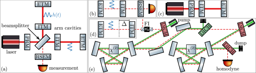
To date, no post-merger signals have been detected, likely because our quantum noise–limited interferometers are not sensitive enough at kilohertz buikemaSensitivityPerformanceAdvanced2020 ; GW170817properties ; postmerger_long ; postmerger_short . Present kilometre-scale interferometers like LIGO are based on the Fabry-Pérot Michelson Interferometer (FPMI) with Dual-Recycling AdvancedLIGO:2015 ; meersRecyclingLaserinterferometricGravitationalwave1988 ; bond_2010 as shown in Fig. 1a. The beamsplitter held at “dark port” sends the differential (common) optical mode, sensitive to differential (common) length changes in the perpendicular arms, towards the measuring device (back towards the laser) as shown in Fig. 1b (Fig. 1c). Gravitational waves differentially strain the arms by dimensionless $h(t)$ at times $t$ such that they displace the optical phase quadrature $\hat{p}$ at the photodetector from the vacuum $\hat{p}^{(0)}$. The Fourier domain complex component $\tilde{h}$ of a monochromatic signal $h(t)$ at a positive angular frequency $\Omega$ is

$$\tilde{h}=\pi T(A+iB),\quad h(t)=A\cos(\Omega t)+B\sin(\Omega t).$$ (1)

Here, $A$ and $B$ are the independent signal degrees-of-freedom at $\Omega$ corresponding to the cosine and sine phases in the time domain, and $T$ is the finite integration time. We can describe the lossless interferometer with the interaction Hamiltonian $\hat{H}_{\text{int}}=gh(t)\hat{x}^{\text{(cav)}}$ where $g$ is the effective coupling rate (given free masses in the transverse-traceless gauge) and $\hat{x}^{\text{(cav)}}$ is the optical amplitude quadrature of the intracavity differential mode kimble_2001 . Using the input/output formalism gardiner1985input , the quadrature $\hat{x}_{\theta}=\cos(\theta)\hat{x}+\sin(\theta)\hat{p}$ at angle $\theta$ of the outgoing field is

$$\hat{x}_{\theta}(\Omega)=d_{\theta}\tilde{h}\hat{1}+\hat{x}_{\theta}^{(0)}(\Omega).$$ (2)

Here, $d_{\theta}$ is the complex linear signal response with $d_{0}=0$ and $\hat{1}$ is the identity operator. To measure a given $\hat{x}_{\theta}$, balanced homodyne readout is planned as a future upgrade to LIGO fritschel2014balanced . We detail the full Hamiltonian model in the Supplemental Material SupplementalMaterial . The resonant-sideband-extraction cavity shown in Fig. 1a trades off the peak sensitivity to increase the bandwidth meersRecyclingLaserinterferometricGravitationalwave1988 ; 1995AuJPh..48..953M , while the power recycling and arm cavities increase the circulating power and sensitivity bond_2010 . Practical challenges with further increasing the circulating power Brooks_2021 ; PhysRevLett.114.161102 ; Barsotti_2018 motivate alternatives to improve the kilohertz sensitivity which is limited by the arm cavities’ bandwidth and quantum shot noise $\text{Var}\mathopen{}\mathclose{{}\left[\hat{p}^{(0)}}\right]$ arising from the Poissonian statistics of the photon number operator buikemaSensitivityPerformanceAdvanced2020 ; PhysRevD.23.1693 ; danilishinQuantumMeasurementTheory2012 .

Detuning the arm cavities of a gravitational-wave interferometer differentially away from the carrier frequency could improve the kilohertz sensitivity Miao+2017 ; PhysRevD.103.022002 ; ward2010length ; somiya2012detector ; miyakawa2006measurement ; buonanno2003scaling ; corbitt2004quantum ; Ganapathy_2021 . The sensitivity improves resonantly around the kilohertz detuning frequency $\Delta$, e.g. $2\pi\times 3000$ Hz, and the quadratures are mixed such that $d_{0}\neq 0$ in Eq. 2 SupplementalMaterial . We consider the more general sensing problem of probing a classical force with a detuned cavity. This is equivalent under the single-mode approximation walls_1995 (which is valid at frequencies well below the free spectral range at of 37.5 kHz for LIGO AdvancedLIGO:2015 ) to gravitational-wave detection using a Detuned Power-Recycled FPMI as shown in the top-left of Fig. 1d. (We describe later how to extend our approach to other configurations including a Detuned Dual-Recycled FPMI.) The sensitivity bounds of this force-sensing problem are not well-established and the optimal measurement scheme is unknown. Moreover, an unexplained sensitivity gap exists between the present measurement scheme and a fundamental limit. We address these points in this Letter.

The gap.—The theory of quantum multi-parameter estimation Holevo2011book ; WisemanMilburn2009book provides the fundamental precision limits on any measurement scheme to estimate $h(t)$ for all $t$. Or, equivalently for a fixed positive frequency $\Omega$, the limits on simultaneously estimating $A$ and $B$ in Eq. 1 using unbiased estimates $\hat{A}$ and $\hat{B}$, respectively. Our figure-of-merit for this estimation procedure is the weighted mean squared estimation error $\Sigma$ where

$$\Sigma =\text{Tr}\mathopen{}\mathclose{{}\left[\text{W}\text{V}}\right],\;\text{W}=\text{diag}\mathopen{}\mathclose{{}\left(2w,\;2\mathopen{}\mathclose{{}\left(1-w}\right)}\right),\;w\in(0,1).$$ (3)

Here, V is the covariance matrix of the estimates and W is the weight matrix: a positive matrix with $\text{Tr}\mathopen{}\mathclose{{}\left[\text{W}}\right]=2$ which is diagonal without loss of generality. The weight may be unequal ($w\neq\frac{1}{2}$) due to a non-uniform prior on the phase, e.g. from the early warning of a future low-frequency space-based gravitational-wave detector gair2013testing ; shaddock2008space ; gong2021concepts ; PhysRevD.102.043001 ; Sedda_2020 . Or, it can be unequal due to a biased ultimate parameter-of-interest, e.g. estimating the signal’s power $\lvert\tilde{h}\rvert^{2}\propto A^{2}+B^{2}$ where $\partial_{A}\lvert\tilde{h}\rvert^{2}$ and $\partial_{B}\lvert\tilde{h}\rvert^{2}$ are unequal and similarly for the true phase $\arg(\tilde{h})=\arctan(B/A)$. Solving this weighted estimation problem is a precursor to studying adaptive measurement schemes. E.g., we could start with equal weights, then continuously update the weights and the measurement as an estimate of the true phase accumulates and eventually converges to single-parameter estimation (where $w=0$ or 1 without loss of generality).

Ref. Miao+2017 computed one such precision limit, the Quantum Cramér-Rao Bound (QCRB) $\Sigma_{Q}$ braunstein1994statistical ; WisemanMilburn2009book , on the error $\Sigma$ in Eq. 3 and found a gap $\Sigma>\Sigma_{Q}$. Unlike our formalism above, Ref. Miao+2017 implicitly worked with equal weights and considered the power spectral density $S=\frac{1}{\pi T}\Sigma$ and the waveform-estimation QCRB $S_{Q}=\frac{1}{\pi T}\Sigma_{Q}$ derived from the fluctuations of $\hat{x}(\Omega)$ Tsang+2011 ; SupplementalMaterial ; the advantages of our formalism will be seen shortly. Unlike the QCRB, the Classical Cramér-Rao Bound (CCRB) is dependent on the measurement scheme and is always saturated for Gaussian displacement like that in Eq. 2 WisemanMilburn2009book . The QCRB is only necessarily saturated for single-parameter estimation where it is equivalent to optimising the CCRB over all possible measurement schemes. Ref. Miao+2017 found a gap of upwards of a factor of two in power units — greatest at the detuning frequency — for the standard “variational readout” scheme in which $A$ and $B$ are estimated from the real and imaginary parts of $\hat{x}_{\theta}(\Omega)$ with $\theta(\Omega)$ optimised for each $\Omega$. This measurement scheme, which is planned as an future upgrade to LIGO, can be realised by homodyne measurement with a frequency-dependent relative phase between the output beam and local oscillator kimble_2001 . If variational readout is not the optimal measurement scheme, then a gain is possible of upwards of $2^{\frac{3}{2}}$ in the volume of the Universe searched for binary neutron-star mergers. In this Letter, we will resolve this gap issue, find the optimal measurement scheme, and show that such a gain is possible.

A toy model.—The multi-parameter QCRB can be loose because it does not address incompatible estimates Holevo2011book . In our formalism, while the signal $\tilde{h}(\Omega)$ has two independent degrees-of-freedom at each positive frequency $\Omega$, the output light has four independent degrees-of-freedom: $\hat{x}(t)$ and $\hat{p}(t)$ oscillating as $\cos(\Omega t)$ and $\sin(\Omega t)$ each, or, equivalently,

$$\vec{\hat{q}}=\frac{1}{\sqrt{\pi T}}\mathopen{}\mathclose{{}\left[\;\begin{matrix}\text{Re}\mathopen{}\mathclose{{}\left[\hat{x}(\Omega)}\right]\\ \text{Re}\mathopen{}\mathclose{{}\left[\hat{p}(\Omega)}\right]\\ \text{Im}\mathopen{}\mathclose{{}\left[\hat{x}(\Omega)}\right]\\ \text{Im}\mathopen{}\mathclose{{}\left[\hat{p}(\Omega)}\right]\end{matrix}\;}\right]=A\vec{d}_{A}\hat{1}+B\vec{d}_{B}\hat{1}+\vec{\hat{q}}^{\,(0)}.$$ (4)

Here, $\vec{d}_{A}$ and $\vec{d}_{B}$ are the linear signal displacements which are orthogonal, have common Euclidean norm $\eta$ such that the QCRB ($\Sigma_{Q}=\eta^{-2}$) is weight-invariant, and have support in all four components SupplementalMaterial . $\vec{\hat{q}}$ constitutes two harmonic oscillators in the ground state since the nonzero commutators of its components ${\vec{\hat{q}}}_{j}$ are

$$[{\vec{\hat{q}}}_{1},{\vec{\hat{q}}}_{2}]=[{\vec{\hat{q}}}_{3},{\vec{\hat{q}}}_{4}]=i$$ (5)

and the covariance matrix of the noise $\vec{\hat{q}}^{\,(0)}$ is $\text{diag}\mathopen{}\mathclose{{}\left(\frac{1}{2},\frac{1}{2},\frac{1}{2},\frac{1}{2}}\right)$ with the reduced Planck constant $\hbar=1$. The optimal individual unbiased estimates for $A$ and $B$, respectively, are

$$\hat{A}_{\text{only}} =\frac{\vec{d}_{A}\cdot\vec{\hat{q}}}{\eta^{2}},\quad\hat{B}_{\text{only}}=\frac{\vec{d}_{B}\cdot\vec{\hat{q}}}{\eta^{2}}$$ (6)

which are incompatible since

$$[\hat{A}_{\text{only}},\hat{B}_{\text{only}}] =\frac{-i\mu}{\eta^{2}},\quad\mu=\frac{2\Delta\Omega}{\gamma^{2}+\Delta^{2}+\Omega^{2}}\in(0,1).$$ (7)

Here, $\gamma$ is the arm cavity’s half-width at half-maximum (HWHM) bandwidth, and the commutator factor $\mu\approx 1$ at $\Omega=\Delta$. The QCRB assumes compatibility a priori, but, in reality, the error is higher since noise must be added to construct compatible estimates. This is the origin of the sensitivity gap in Ref. Miao+2017 .

Consider an analogy to a toy model. The detuned interferometer at each positive frequency constitutes two harmonic oscillators displaced from the vacuum by two incompatible signals. To simplify the representation, we can symplectically transform the normalised displacements (preserving their commutator up to a sign) to

$$\vec{n}_{A} =\frac{\text{M}\vec{d}_{A}}{\eta},\quad\vec{n}_{B}=\frac{\text{M}\vec{d}_{B}}{\eta}$$ (8)

$$\mathopen{}\mathclose{{}\left[\vec{n}_{A}\cdot\vec{\hat{X}},\vec{n}_{B}\cdot\vec{\hat{X}}}\right] =\mathopen{}\mathclose{{}\left[\hat{X}_{1},\mu\hat{P}_{1}+\sqrt{1-\mu^{2}}\hat{X}_{2}}\right]=i\mu.$$ (9)

Here, the symplectic 4-by-4 matrix M is unique and $\vec{\hat{X}}=(\hat{X}_{1},\hat{P}_{1},\hat{X}_{2},\hat{P}_{2})^{\text{T}}$ are the toy model quadratures with rescaled signals $A^{\prime}=\eta A$ and $B^{\prime}=\eta B$ such that SupplementalMaterial

$$\vec{\hat{X}} =\text{M}\vec{\hat{q}}=A^{\prime}\vec{n}_{A}\hat{1}+B^{\prime}\vec{n}_{B}\hat{1}+\vec{\hat{X}}^{(0)}.$$ (10)

The incompatible displacements should not be confused with those acting on each oscillator. The analogous error $\Sigma^{\prime}=\eta^{2}\Sigma$ with respect to $A^{\prime}$ and $B^{\prime}$ is given via the chain rule $\partial_{A}=\eta\,\partial_{A^{\prime}}$.

Results for the toy model.—The tight bound for simultaneous compatible multi-parameter estimation is the Holevo Cramér-Rao Bound (HCRB) $\Sigma_{H}^{\prime}$ Holevo2011book ; Genoni+2013 ; Bradshaw+2017 ; Bradshaw+2018 . Intuitively, the HCRB is defined by minimising the QCRB over all unbiased estimates plus a penalty for incompatibility. It is equivalent to finding the optimal “Quantum Mechanics–free subspace” where the displacements are orthogonal and commute tsang2012evading . For the Gaussian displacements in Eq. 10, the HCRB is saturated by the optimal compatible linear combinations of $\vec{\hat{X}}$ Holevo2011book . This means that calculating the HCRB can be expressed as a semi-definite program, here involving four-by-four real matrices Bradshaw+2018 ; doi:10.1137/1038003 . We calculate the HCRB from Eq. 10 using the method from Ref. Bradshaw+2017 . In the Supplemental Material SupplementalMaterial , we show that the HCRB reduces to single-parameter optimisation — despite requiring solving a semi-definite program a priori

$$\Sigma_{H}^{\prime} =\min_{\phi\in(0,\pi]}\mathopen{}\mathclose{{}\left(\frac{w}{\cos(\phi)^{2}}+\frac{1-w}{\cos(\phi+\arcsin(\mu))^{2}}}\right)$$ (11)

and we find analytic solutions in certain limits

$$\Sigma_{H}^{\prime} {=}1+2\sqrt{w(1-w)},\,\;\;\Sigma_{H}^{\prime}\overset{w=\frac{1}{2}}{=}\frac{2}{1+\sqrt{1-\mu^{2}}}.$$ (12)

This generalizes previous results to arbitrary commutator and weight. Genoni+2013 ; Bradshaw+2017 ; Bradshaw+2018 .

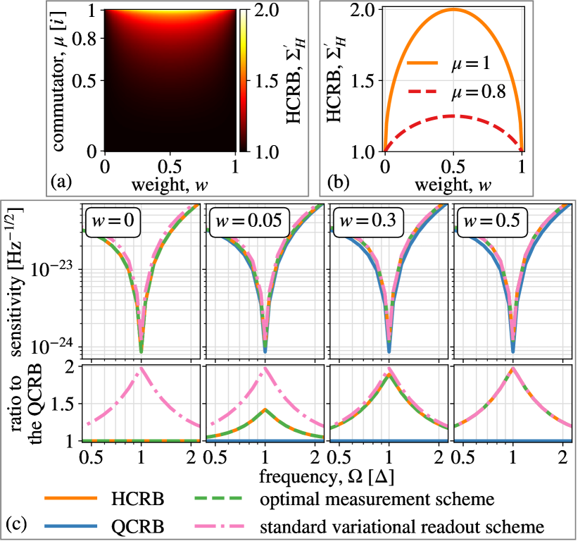
Fig. 2a shows the HCRB in Eq. 11 versus $w$ and $\mu$. In comparison, for the toy model, the QCRB is uniformly unity ($\Sigma_{Q}^{\prime}\equiv 1$) from measuring both harmonic oscillators with a vacuum variance of $\frac{1}{2}$ each. The HCRB has value $\Sigma_{H}^{\prime}\in(1,2)$, depends positively and monotonically on $\mu$, and has a symmetric concave-down profile in $w$ for fixed $\mu$ as shown in Fig. 2b. The HCRB decreases with less equal weights because another Quantum Mechanics–free subspace has less noise by compromising the less important signal phase. The HCRB is unity at $w=0$ or $w=1$ because it reduces to the QCRB for single-parameter estimation.

The optimal compatible measurements are SupplementalMaterial

$$\hat{T}_{1} =\cos(\mkern 1.5mu\overline{\mkern-1.5mu\phi\mkern-1.5mu}\mkern 1.5mu)\hat{X}_{1}-\sin(\mkern 1.5mu\overline{\mkern-1.5mu\phi\mkern-1.5mu}\mkern 1.5mu)\hat{P}_{2}$$ (13)

$$\hat{T}_{2} =\cos(\mkern 1.5mu\overline{\mkern-1.5mu\phi\mkern-1.5mu}\mkern 1.5mu)\hat{X}_{2}-\sin(\mkern 1.5mu\overline{\mkern-1.5mu\phi\mkern-1.5mu}\mkern 1.5mu)\hat{P}_{1}$$ (14)

where $\mkern 1.5mu\overline{\mkern-1.5mu\phi\mkern-1.5mu}\mkern 1.5mu$ is the optimal angle in Eq. 11. The optimal compatible unbiased estimates for $A^{\prime}$ and $B^{\prime}$, respectively, whose error $\Sigma^{\prime}$ saturates the HCRB $\Sigma^{\prime}_{H}$ in Eq. 11 are

$$\hat{A}^{\prime}=\frac{1}{\cos\mathopen{}\mathclose{{}\left(\mkern 1.5mu\overline{\mkern-1.5mu\phi\mkern-1.5mu}\mkern 1.5mu}\right)}\hat{T}_{1},\quad\hat{B}^{\prime}=\frac{1}{\cos\mathopen{}\mathclose{{}\left(\mkern 1.5mu\overline{\mkern-1.5mu\phi\mkern-1.5mu}\mkern 1.5mu+\arcsin(\mu)}\right)}\hat{T}_{2}.$$ (15)

Precision limits of detuned interferometry.—We use the analogy to the toy model to analyse the detuned interferometer at each positive frequency. For similar detuned cavity–based systems, e.g. a Detuned Dual-Recycled FPMI, another analogy to the toy model exists with different $\mu$ and $\eta$ etc. such that the same method will suffice. The HCRB for simultaneous estimation of $A$ and $B$ for the detuned interferometer is $\Sigma_{H}=\eta^{-2}\Sigma_{H}^{\prime}$ by the chain rule, such that the gap to the QCRB of $\Sigma_{Q}=\eta^{-2}$ is $\Sigma_{H}^{\prime}$. The optimal compatible estimates $\hat{A}=\eta^{-1}\hat{A}^{\prime}$ and $\hat{B}=\eta^{-1}\hat{B}^{\prime}$ of $A$ and $B$, respectively, are linear combinations of $\vec{\hat{q}}$ by Eq. 15. In comparison, the standard variational readout scheme estimates $A$ ($B$) from $\text{Re}\mathopen{}\mathclose{{}\left[\hat{x}_{\theta}(\Omega)}\right]$ ($\text{Im}\mathopen{}\mathclose{{}\left[\hat{x}_{\theta}(\Omega)}\right]$) which is restricted to the inner product of $[\cos(\theta),\sin(\theta)]$ and $[{\vec{\hat{q}}}_{1},{\vec{\hat{q}}}_{2}]$ ($[{\vec{\hat{q}}}_{3},{\vec{\hat{q}}}_{4}]$).

Figure 2: (a) HCRB versus the commutator and weight for the toy model. (b) HCRB versus the weight for the toy model with different commutators. (c, top row) Strain sensitivity for the detuned interferometer in effective amplitude spectral density units versus frequency for the parameters in Table 1 and different weights $w$. The behaviour is symmetric about $w=\frac{1}{2}$. (c, bottom row) The ratio of the above sensitivity to the QCRB in power units versus frequency.

arm cavity length	4 km	carrier frequency	$282$ THz
HWHM bandwidth	$42$ Hz	circulating power	750 kW
detuning frequency	$3$ kHz	ITM power transmitted	0.014

Table 1: Parameters from Advanced LIGO AdvancedLIGO:2015 for the Detuned Power-Recycled FPMI configuration shown in Fig. 1d.

Arbitrary linear combinations of $\vec{\hat{q}}$ are non-stationary such that the power spectral density is not formally defined. To compare the performance to the sensitivity of the standard variational readout scheme and the waveform-estimation QCRB Miao+2017 , however, we can define effective values for the power spectral density of the optimal estimates $S=\frac{1}{\pi T}\Sigma$ and the waveform-estimation HCRB $S_{H}=\frac{1}{\pi T}\Sigma_{H}$ SupplementalMaterial . In Fig. 2c, we show that for equal weights the standard variational readout scheme saturates the HCRB such that the gap to the QCRB is insurmountable. For unequal weights, however, a new scheme measuring the optimal estimates improves the sensitivity and is required to saturate the HCRB. For $w=0.05$ or $0.95$, this scheme could provide a sensitivity gain of approximately $\sqrt{2}$ in power units corresponding to a gain of 68% in the volume of the Universe searched for post-merger signals as shown in Fig. 2c. This increases to upwards of a factor of two in power units and 183% in volume for $w=\varepsilon$ or $1-\varepsilon$ with $0<\varepsilon\ll 1$ close to single-parameter estimation. Such weights arise from a strong prior on the phase or strongly biased ultimate parameter-of-interest.

Proposal for an experimental realisation.—We propose how to realise the optimal measurement scheme at a given $\Omega=\Delta$ for any $\mu$ and $w$. By expanding $\vec{\hat{q}}$ into the time domain, the optimal estimates are SupplementalMaterial

$$\hat{A} =\int_{-\infty}^{\infty}\text{d}t\;c_{A}(t)\hat{x}_{\vartheta_{A}(t)}(t)$$ (16)

$$\hat{B} =\int_{-\infty}^{\infty}\text{d}t\;c_{B}(t)\hat{x}_{\vartheta_{B}(t)}(t).$$ (17)

For $w=1$ ($w=0$), therefore, an individual measurement of $\hat{A}$ ($\hat{B}$) can be realised with homodyne readout using a local oscillator with phase $\vartheta_{A}(t)$ ($\vartheta_{B}(t)$) modulated at $\Delta$ by integrating the measured timeseries against the kernel $c_{A}(t)$ ($c_{B}(t)$). Although the integrated estimates are compatible, their integrands in Eq. 16 may not commute at a given time $t$. This prevents simultaneously performing naïve homodyne measurements of $\hat{A}$ and $\hat{B}$. An asymmetric beamsplitter can introduce an auxiliary mode to compensate for the commutator of $\hat{A}_{\text{only}}$ and $\hat{B}_{\text{only}}$ at each time, but this only works for $\mu=1$ SupplementalMaterial . The individual homodyne measurement of $\hat{A}$ above, however, only used the DC Fourier component of the timeseries times $c_{A}(t)$. Since the $2\Delta$ Fourier component beats with the homodyne measurement oscillating at $\Delta$, it is a linear combination of the quadratures at the difference ($\Delta$) and sum ($3\Delta$) frequencies. This can realise a heterodyne measurement of $\hat{B}$ at $\Delta$ but with added noise at $3\Delta$ buonanno2003quantum ; SupplementalMaterial . Using quantum squeezing in two cascaded, detuned, and narrowband filter cavities as shown in Fig. 1e, this heterodyne noise at $3\Delta$ can be squeezed without affecting the estimates at $\Delta$ SupplementalMaterial . We can saturate the HCRB at $\Omega=\Delta$ for any $\mu$ and $w$ using a homodyne measurement of $\hat{A}$ and a heterodyne measurement of $\hat{B}$ with no added noise. We emphasise that squeezing the output beam does not change the HCRB and is only used to demonstrate that the measurement scheme is realisable. In practice, the input beam into the dark port of the interferometer can also be squeezed, which will improve the precision limits aasietal2013 ; tseQuantumEnhancedAdvancedLIGO2019 ; mcculler2020frequency .

Conclusions and outlook.—In this Letter, we found the optimal measurement scheme to improve the precision of detuned cavity–based quantum sensors. In particular, we can improve the sensitivity of detuned gravitational-wave interferometers to the elusive post-merger signals from binary neutron-star mergers. Previous work on detuned interferometers found an unexplained gap of up to a factor of two in power units between the sensitivity of the standard variational readout scheme and the QCRB. We resolved this gap. We showed that it stems from the incompatibility of the naïve estimates of the cosine and sine phases of the signal at each frequency. This observation allowed us to rigorously establish the attainable precision limit and find the optimal measurement scheme. For an equal weighting between the phases, we proved that the gap cannot be overcome and the standard homodyne measurement is indeed optimal. In the unequal weight regime, however, the sensitivity can be improved by using a different measurement scheme which we propose how to experimentally realise. This regime could arise from a non-uniform prior, a biased ultimate parameter-of-interest, or using an adaptive protocol. This new scheme could significantly increase the volume of the Universe searched for post-merger signals in this regime and possibly have other applications to detuned cavity–based quantum metrology.

We defer to future work realising a broadband optimal measurement scheme for any $\mu$ and $w$ without squeezing the output beam, but perhaps squeezing the input beam appropriately. Future work should also rigorously show that an adaptive protocol can close the sensitivity gap by continuously updating the weights to converge to single-parameter estimation. Our analogy to the toy model could also be extended to detuned cavity–based systems with additional output degrees-of-freedom, e.g. to improve the sensitivity of detuned $\mathcal{PT}$-symmetric interferometers and axion detectors Wang+2022 ; Metelmann+2014 ; li2020broadband ; liEnhancingInterferometerSensitivity2021 ; Bentley+2021arXiv ; PhysRevD.106.L041101 ; PhysRevLett.51.1415 ; PhysRevLett.124.101303 ; PhysRevX.9.021023 ; MARSH20161 .

Our code is available online FIrepo and was written using Mathematica mathematica and Python python ; ipython ; jupyter ; numpy ; matplotlib .