Population synthesis of Be X-ray binaries: metallicity dependence of total X-ray outputs

Abstract

X-ray binaries (XRBs) are thought to regulate cosmic thermal and ionization histories during the Epoch of Reionization and Cosmic Dawn ($z\sim 5-30$). Theoretical predictions of the X-ray emission from XRBs are important for modelling such early cosmic evolution. Nevertheless, the contribution from Be-XRBs, powered by accretion of compact objects from decretion disks around rapidly rotating O/B stars, has not been investigated systematically. Be-XRBs are the largest class of high-mass XRBs (HMXBs) identified in local observations and are expected to play even more important roles in metal-poor environments at high redshifts. In light of this, we build a physically motivated model for Be-XRBs based on recent hydrodynamic simulations and observations of decretion disks. Our model is able to reproduce the observed population of Be-XRBs in the Small Magellanic Cloud with appropriate initial conditions and binary stellar evolution parameters. We derive the X-ray output from Be-XRBs as a function of metallicity in the (absolute) metallicity range $Z\in[10^{-4},0.03]$ with a large suite of binary population synthesis (BPS) simulations. The simulated Be-XRBs can explain a non-negligible fraction ($\gtrsim 30\%$) of the total X-ray output from HMXBs observed in nearby galaxies for $Z\sim 0.0003-0.02$. The X-ray luminosity per unit star formation rate from Be-XRBs in our fiducial model increases by a factor of $\sim 8$ from $Z=0.02$ to $Z=0.0003$, which is similar to the trend seen in observations of all types of HMXBs. We conclude that Be-XRBs are potentially important X-ray sources that deserve greater attention in BPS of XRBs.

1 Introduction

During the Epoch of Reionization and Cosmic Dawn ($z\sim 5-30$), X-ray binaries (XRBs) are expected to be the dominant sources of X-rays that regulate the thermal and ionization evolution and small-scale structure of the interstellar medium (IGM, e.g., Fragos et al., 2013b; Fialkov et al., 2014; Fialkov & Barkana, 2014; Pacucci et al., 2014; Madau & Fragos, 2017; Eide et al., 2018), as well as early star formation (e.g., Jeon et al., 2012; Artale et al., 2015; Hummel et al., 2015; Ricotti, 2016; Park et al., 2021a, b, 2023b). They can leave unique signatures in the 21-cm signal from neutral hydrogen, which is one of the most promising probes of early structure/galaxy/star formation and cosmology (e.g., Fialkov et al., 2017; Bowman et al., 2018; Ewall-Wice et al., 2018; Ma et al., 2018; Madau, 2018; Mirocha & Furlanetto, 2019; Schauer et al., 2019; Chatterjee et al., 2020; Qin et al., 2020; Gessey-Jones et al., 2022; Kamran et al., 2022; Kaur et al., 2022; Kovlakas et al., 2022; Magg et al., 2022; Muñoz et al., 2022; Acharya et al., 2023; Bevins et al., 2023; Hassan et al., 2023; Lewis et al., 2023; Ma et al., 2023; Mondal & Barkana, 2023; Shao et al., 2023; Ventura et al., 2023; Yang et al., 2023), and in the Lyman-$\alpha$ forest from long-lasting relics of reionization (Montero-Camacho et al., 2023). To fully unleash the power of the 21-cm probe and break potential degeneracy between astrophysics, dark matter physics and cosmology (e.g., Barkana, 2018; Liu et al., 2019; Yang, 2021; Yang et al., 2023; Ghara et al., 2022; Acharya et al., 2023; Mondal et al., 2023; Shao et al., 2023), it is necessary to model the X-ray emission from XRBs accurately.

The metallicity dependence of X-ray outputs from high-mass XRBs (HMXBs, reviewed by, e.g., Walter et al., 2015; Kretschmar et al., 2019; Fornasini et al., 2023), which dominate the cosmic XRB luminosity density at $z\gtrsim 3$ (Fragos et al., 2013a), is particularly important in the early Universe when the metal content of XRB host galaxies evolves rapidly (e.g., Wise et al., 2012; Johnson et al., 2013; Xu et al., 2013; Pallottini et al., 2014; Liu & Bromm, 2020; Ucci et al., 2023), and the X-rays from active galactic nuclei are subdominant (see, e.g., Fragos et al., 2013b). In fact, X-ray observations of nearby and distant (up to $z\sim 2$) galaxies (e.g., Antoniou et al., 2010; Antoniou et al., 2019; Basu-Zych et al., 2013; Prestwich et al., 2013; Douna et al., 2015; Antoniou & Zezas, 2016; Brorby et al., 2016; Lehmer et al., 2016, 2019, 2021; Lehmer et al., 2022; Aird et al., 2017; Fornasini et al., 2019, 2020; Riccio et al., 2023) and theoretical predictions by binary population synthesis (BPS) of XRBs (e.g., Linden et al., 2010; Fragos et al., 2013b; Sartorio et al., 2023) all suggest a strong metallicity dependence of the X-ray output from HMXBs. This drives the redshift evolution of the scaling relation between X-ray luminosity and star formation rate (SFR), and can have significant impact on the 21-cm signal (e.g., Kaur et al., 2022). For instance, Fragos et al. (2013b) provides fitting formulae for the X-ray luminosity of HMXBs per unit SFR as a function of metallicity from BPS simulations (Fragos et al., 2013a). In their case, the X-ray luminosity increases by a factor of $\sim 6$ from solar metallicity to $\sim$1% solar, consistent with the trend seen in observations. Sartorio et al. (2023) derives the X-ray outputs of XRBs from metal-free stars, i.e., the so-called Population III (Pop III). They find that in optimistic cases the X-ray emission of Pop III XRBs can be significantly stronger (up to a factor of 40) compared with that of XRBs from metal-enriched stars predicted by Fragos et al. (2013b).

However, the aforementioned BPS studies only consider the XRBs powered by Roche lobe overflow (RLO) and (spherical) stellar winds but ignore an important type of HMXBs, Be-XRBs, likely due to their transient nature. A Be-XRB is made of a compact object and a rapidly-rotating, massive ($\gtrsim 6\ \rm M_{\odot}$), main sequence (MS) star (reviewed by, e.g., Reig, 2011; Rivinius et al., 2013; Rivinius, 2019). Here the massive star is typically of spectral type B (and O) with an rotation velocity above $\sim 70$ percent of the equatorial Keplerian limit and shows Balmer emission lines, which can be well explained by a viscous decretion disk (VDD) around the star. This VDD is formed by materials ejected from the star due to redistribution of angular momentum caused by fast rotation (Rivinius et al., 2013). In most observed Be-XRBs, neutron stars (NSs) are identified as the compact companion, although there are two binaries, MWC 656 and AS 386, that contain a Be star and a black hole (BH) candidate but show very faint X-ray emission (Casares et al., 2014; Munar-Adrover et al., 2014; Grudzinska et al., 2015; Khokhlov et al., 2018; Zamanov et al., 2022), and one Be-XRB that contains a white dwarf (Swift J011511.0-725611, Kennea et al., 2021). The X-ray output of Be-XRBs is dominated by X-ray outbursts produced by strong accretion of the compact object from the VDD, which typically occurs close to periastron (Okazaki, 2001; Okazaki & Negueruela, 2001) and/or when the compact object crosses a tidally warped (eccentric) VDD (Okazaki et al., 2013; Franchini & Martin, 2021).

Be-XRBs make up the largest class of HMXBs identified in observations (Fornasini et al., 2023), especially in metal-poor environments. In the Milky Way (MW), 74 Be-XRBs have been found among the total 152 known HMXBs (Fortin et al., 2023). In the Large Magellanic Cloud (LMC) at approximately half solar metallicity, there are 33 Be-XRBs among the 40 confirmed HMXBs (Antoniou & Zezas, 2016), while in the Small Magellanic Cloud (SMC) at about one quarter solar metallicity, 69 X-ray pulsars are identified as Be-XRBs among the 121 HMXB candidates (Coe & Kirk, 2015; Haberl & Sturm, 2016). The HMXB population of M33 is also dominated by Be-XRBs (Lazzarini et al., 2023). Besides, theoretical models find that Be-XRBs can be an important component of the X-ray luminosity function of HMXBs in the MW (Zuo et al., 2014; Misra et al., 2023b). However, previous BPS studies of Be-XRBs (e.g., Zhang et al., 2004; Belczynski & Ziolkowski, 2009; Linden et al., 2009; Shao & Li, 2014, 2020; Zuo et al., 2014; Vinciguerra et al., 2020; Xing & Li, 2021; Misra et al., 2023b) focus on the cases of solar and SMC metallicities in which they either do not model the X-ray emission or use rough estimates and empirical scaling laws to characterize the VDDs and X-ray outbursts of Be-XRBs (e.g., Dai et al., 2006; Coe & Kirk, 2015; Klement et al., 2017). The overall X-ray outputs from Be-XRB populations as a function of metallicity has not been investigated quantitatively, while a strong metallicity dependence is expected from the reduced mass loss at low metallicities (Linden et al., 2010; Fragos et al., 2013a; Sartorio et al., 2023). Therefore, it is crucial to include Be-XRBs in BPS models to evaluate the metallicity dependence of X-ray outputs from the entire population of HMXBs.

In light of the potential importance of Be-XRBs for the cosmic thermal and ionization history, we build a physically motivated Be-XRB model to predict the X-ray output from Be-XRBs as a function of metallicity with BPS. Inspired by the recent advancements in hydrodynamic simulations of VDDs in Be-XRBs (Okazaki et al., 2013; Panoglou et al., 2016; Cyr et al., 2017; Brown et al., 2018, 2019; Suffak et al., 2022), our model fully captures for the first time the dependence of X-ray outburst properties (i.e., strength and duty cycle) on stellar and orbital parameters of Be-XRBs by combining simulation results (Brown et al., 2019) with VDD properties inferred from observations of Be stars (Vieira et al., 2017; Rímulo et al., 2018). In this paper we focus on the absolute metallicity range $Z\in[10^{-4},0.03]$ where observational constraints for HMXBs are available. Our model can also be applied to more metal-poor regimes (e.g., $Z\lesssim 10^{-6}$ for Pop III stars) that are likely more important at Cosmic Dawn (Sartorio et al., 2023).

The paper is structured as follows. In Section 2, we provide an overview of our method and discuss the setup of BPS parameters, binary sample and initial conditions. In Section 3, we explain our physically motivated model for the identification and characterization of Be-XRBs. In Section 4, we build a empirical model for the X-ray spectra of Be-XRBs. In Section 5 we present our predictions on the formation efficiency (Sec. 5.1), mass and orbital parameter distributions (Sec. 5.2), and X-ray outputs of Be-XRBs (Sec. 5.3), focusing on how they evolve with metallicity. Finally, we summarize our main findings in Section 7, and discuss their caveats and our outlook to future work in Section 6. The key physical quantities used in this paper are summarized in Table 1.

Table 1: Key physical quantities.

$Z$	absolute metallicity (mass fraction of metals)
$M_{1}$	initial primary mass
$M_{2}$	initial secondary mass
$a$	orbital separation (semi-major axis)
$e$	orbital eccentricity
$P_{\rm orb}$	orbital period
$P_{\rm s}$	spin period of the NS
$M_{\rm X}$	compact object (NS/BH) mass
$M_{\star}$	mass of the donor star
$R_{\star}$	equatorial radius of the donor star
$v_{\rm Kep}$	equatorial Keplerian velocity of the donor star
$v_{\rm rot}$	equatorial rotation velocity of the donor star
$W$	$\equiv v_{\rm rot}/v_{\rm Kep}$ with the initial value denoted by $W_{0}$
$R_{\rm L1}$	Roche lobe size of the donor star at periastron (Eq. 6)
$R_{\rm trunc}$	$\equiv f_{\rm trunc}a$, average tidal truncation radius (Eq. 7)
$R_{\rm crit}$	VDD boundary beyond which gas flows are subsonic (Eq. 8)
$c_{s}$	sound speed in the ionised isothermal VDD
$\Sigma_{0}$	base surface density of the VDD
$\alpha$	viscosity parameter of the VDD
$\dot{M}_{\rm ej}$	mass ejection rate of the O/B star
$\dot{M}_{\rm acc}$	peak/outburst accretion rate in the Be-XRB
$L_{\rm bol}$	bolometric luminosity during outbursts
$\epsilon$	radiative efficiency
$\dot{M}_{\rm Edd}$	Eddington limit of accretion rate (Eq. 15)
$\eta$	$\equiv\dot{M}_{\rm acc}/\dot{M}_{\rm Edd}$, Eddington ratio during outbursts
$f_{\rm duty}$	effective fraction of time the Be-XRB spends in outbursts
$L_{\rm X}$	outburst X-ray luminosity for a certain band
$\psi_{\rm X}$	calibration parameter for the observed $L_{\rm X}-P_{\rm orb}$ relation
$f_{\rm corr}$	correction factor for outburst luminosity (Sec. 3.2)
$\tau$	lifetime of the Be-XRB
$M_{\rm tot}$	total stellar mass underlying the Be-XRB population
$\mathcal{N}_{\rm X}$	number of Be-XRBs in the outburst phase per unit SFR
$\mathcal{L}_{\nu}$	specific X-ray luminosity per unit SFR
$\mathcal{L}_{\rm X}$	X-ray luminosity per unit SFR for a certain band

2 Binary population synthesis

We add a new module for the identification and characterization of Be-XRBs to the BPS code binary_c (Izzard et al., 2004, 2006, 2009, 2017; Izzard & Halabi, 2018; Izzard & Jermyn, 2023; Mirouh et al., 2023; Hendriks et al., 2023; Hendriks & Izzard, 2023b; Yates et al., 2023), which simulates the evolution of stars in each binary and the binary orbit governed by binary interactions (e.g., mass transfer and tidal effects) and stellar evolution processes such as winds and supernovae (SNe). We evolve large populations of binaries from zero-age main-sequence (ZAMS) for $15$ Gyr in the (absolute) metallicity range $Z\in[10^{-4},0.03]$ with randomly sampled initial binary properties through the python interface binary_c-python (Hendriks & Izzard, 2023a) of binary_c. The Be-XRB model is explained in detail in the next Section 3. An X-ray spectral model based on observations (Sec. 4) is applied to the Be-XRB populations generated by binary_c in post-processing to calculate their X-ray outputs.

As shown in previous BPS studies (e.g., Vinciguerra et al., 2020; Xing & Li, 2021), the main channel of Be-XRB formation is expected to be stable mass transfer during the main sequence (MS) and Hertzsprung gap (HG) phases, where the initial secondary star grows by accretion from the initial primary star and is meanwhile spun up to become an O/Be star. Thereafter, if the initial primary star collapses into a compact object when the O/Be star is still on MS, and the system remains bound, we can obtain a Be-XRB. Therefore, formation of Be-XRBs is sensitive to binary stellar evolution parameters governing the stability and efficiency of mass transfer, angular momentum loss, as well as natal kicks of SNe (see, e.g., Shao & Li, 2014; Vinciguerra et al., 2020; Xing & Li, 2021). The initial binary properties may also play an important role.

In this work, we use the standard BSE models (Hurley et al., 2002) with the default setup of binary_c with an updated stellar wind model from Schneider et al. (2018) and Sander & Vink (2020) as well as a special treatment of mass-transfer efficiency (Sec. 2.1). In addition to the mass-transfer efficiency, we briefly explain our choices of select BSE parameters that are important for Be-XRBs in Sec. 2.2 according to the default setup of binary_c detailed in Izzard et al. (2017). It is shown in Appendix A that our choices of BSE parameters, combined with standard initial conditions of binary stars (Sec. 2.3), can reproduce the population of observed Be-XRBs in the SMC at the metallicity $Z_{\rm SMC}=0.0035$ (Davies et al., 2015). For simplicity, we assume that the BSE parameters and initial conditions do not evolve with metallicity for $Z\in[10^{-4},0.03]$.

The BSE models used here keep track of the spin evolution of each star regulated by mass loss, accretion and tidal interactions, as detailed in Hurley et al. (2002). In particular, during stable mass transfer via RLO, the accretor gains angular momentum from the accreted material, which is assumed to come from the inner edge of an accretion disc with the specific angular momentum of the circular orbit on the surface of the accretor. However, the effects of rotation on stellar evolution are not considered, which can be significant (particularly for initially fast-rotating stars) and complex, covering various aspects (e.g., mass loss, timescales of evolution phases, stellar structure, nucleosynthesis and remnant masses), especially at low $Z$, as shown in detailed stellar-evolution simulations (e.g., Ekström et al., 2012; Georgy et al., 2013; Choi et al., 2017; Groh et al., 2019; Murphy et al., 2021). Such effects may also be important in the modelling of Be-XRBs, as fast-rotating O/B stars are involved by definition. However, it is beyond the scope of this work to take into account these effects because the detailed mechanisms that connect the formation and properties of VDDs (i.e., the so-called ‘Be phenomenon’) with stellar evolution processes are still unresolved (Rivinius et al., 2013).

For simplicity, we ignore the mass growth of compact objects via accretion in Be-XRBs, so that our Be-XRB module does not affect binary stellar evolution. This approximation is justified by the fact that VDDs are very light structures (Rivinius, 2019) that cannot supply much mass to compact objects. We have verified that among all compact objects in the Be-XRBs simulated in this work, the mass accreted from the VDD is less then a few percent of the initial mass in most ($\gtrsim 99\%$) cases, and remains below $50\%$ of the initial mass in the most extreme systems with massive VDDs.

2.1 Mass-transfer efficiency

It is found by Vinciguerra et al. (2020) using the compas code (Riley et al., 2022) that efficient accretion during stable mass transfer is required to reproduce the observed orbital period distribution of Be-XRBs in the SMC. Since compas is also based on the BSE models, we expect that an enhancement of mass-transfer efficiency with respect to the default prescription of binary_c is necessary in our case. Therefore, we set the mass-transfer efficiency parameter, i.e., the ratio of the accreted mass to mass lost by the donor, as

$$\beta=\min\left(1,\beta_{\rm thermal}\times\frac{\dot{M}_{\rm acc,\max}}{\dot{M}_{\rm donor}}\right)\ .$$ (1)

Here $\dot{M}_{\rm donor}$ is the mass loss rate of the donor, $\beta_{\rm thermal}$ is the maximal mass-transfer efficiency defined with respect to the maximal steady-state mass acceptance rate $\dot{M}_{\rm acc,\max}\sim(\epsilon_{\rm g,acc}/L_{\rm acc})^{-1}\sim L_{\rm acc}R_{\rm acc}/(GM_{\rm acc})\sim M_{\rm acc}/t_{\rm KH,acc}$, which is limited by the thermal (Kelvin-Helmholtz) timescale $t_{\rm KH}\sim GM_{\rm acc}^{2}/(R_{\rm acc}L_{\rm acc})$ of the accretor, given $\epsilon_{\rm g,acc}\sim GM_{\rm acc}/R_{\rm acc}$ the specific energy carried by the in-falling matter that needs to be radiated away, the luminosity $L_{\rm acc}$, mass $M_{\rm acc}$ and radius $R_{\rm acc}$ of the accretor. binary_c adopts a conservative choice $\beta_{\rm thermal}=1$ by default, while here we use $\beta_{\rm thermal}=30$, which is approximately the value required to match observations inferred by Vinciguerra et al. (2020). This rather large value of $\beta_{\rm thermal}$ captures the variation of $t_{\rm KH}$ during mass transfer by expansion and increase of luminosity (Paczyński & Sienkiewicz, 1972; Hurley et al., 2002; Vinciguerra et al., 2020). Similarly, we also increase the upper limit on $\beta$ from the dynamical timescale of the accretor as well as the thermal and dynamical timescales of the donor by a factor of 30. Although such efficient mass transfer is required to reproduce the observed Be-XRBs in the SMC (see Appendix A), we find by numerical experiments that the total X-ray output from Be-XRBs is insensitive to $\beta_{\rm thermal}$. The reason is that the total X-ray output is dominated by luminous Be-XRBs mainly on eccentric orbits ($e\gtrsim 0.1$) whose progenitor primary stars only undergo weak mass loss (i.e., $\beta=1$ for $\dot{M}_{\rm donor}\ll\dot{M}_{\rm acc,\max}$, independent of $\beta_{\rm thermal}$), as discussed in Sec. 5.

2.2 Other key BSE parameters

In addition to mass-transfer efficiency, the properties of Be-XRBs are also expected to depend on the prescriptions for mass transfer stability, angular momentum loss, remnant masses and SN natal kicks (Vinciguerra et al., 2020). We plan to explore their effects in the future (see Sec. 6). Here we briefly describe the default choices for these parameters adopted in our work for binary_c.

Mass transfer is stable when $M_{\rm accretor}/M_{\rm donor}>q_{\rm crit}$ at the onset of mass transfer given the critical mass ratio $q_{\rm crit}$. We adopt $q_{\rm crit}=5/8$, 1/3 and 1/4 in the hydrogen MS, helium MS and HG phases for both hydrogen and helium burning of the donor, respectively. In the giant phase, we use the prescription in Hurley et al. (2002, see their sec. 2.6). Mass transfer beyond what is allowed by the mass-transfer efficiency (Eq. 1) is lost from the system. We adopt the fast (also called Jeans) model (Huang, 1963) to calculate the angular momentum loss in this process, i.e., the specific angular momentum carried by the lost mass is equal to the specific angular momentum of the donor. We have verified by numerical experiments using the isotropic re-emission model (Soberman et al., 1997), in which the lost material carries the specific angular momentum of the accretor, that the prescription of angular momentum loss has minor effects on our results (with $\lesssim 20\%$ and $\lesssim 50\%$ changes in the total X-ray output for $Z\lesssim 0.01$ and $Z\sim 0.01-0.03$, respectively). The reason is that under the high mass-transfer efficiency described in Sec. 2.1, the mass/angular momentum loss during stable mass transfer has little impact on the orbital parameters (and luminosities) of Be-XRBs, which are more sensitive to stellar winds and SN natal kicks (see below and Sec. 5.3.1).

The masses of compact object remnants are determined by the CO core masses of progenitors using the original BSE models in Hurley et al. (2000) and Hurley et al. (2002). We apply natal kicks to Type II and Ib/c SNe that follow a Maxwellian distribution with a dispersion of $\sigma_{\rm kick}=190\ \rm km\ s^{-1}$ (Hansen & Phinney, 1997), while electron-capture SNe have no natal kicks. The latter typically happen to highly stripped stars in progenitor binaries of Be-XRBs (see Sec. 5.2), which are expected to have weak natal kicks ($\lesssim 30\ \rm km\ s^{-1}$, see the discussion in sec. 3.1 of Vinciguerra et al., 2020). Therefore, we use zero natal kicks for simplicity.

2.3 Binary sample and initial conditions

To construct the input catalog of binary stars, we sample $N_{\rm B}=3\times 10^{5}$ binaries randomly from widely used distributions of mass and orbital parameters. To be specific, the primary stellar mass $M_{1}$ is drawn from the Kroupa (2001) initial mass function (IMF) in the mass range of $[5,100]\ \rm M_{\odot}$ and the mass ratio $q\equiv M_{2}/M_{1}$ is generated from a uniform distribution in the range $q\in[0.1\ {\rm M_{\odot}}/M_{1},1]$. Here we only consider binaries with $M_{1}\geq 5\ \rm M_{\odot}$ because only massive primary stars can form the compact objects considered in our Be-XRB model (see Sec. 3.1). In the way, the binary stars in our catalog only make up a small fraction of the whole underlying stellar population. Following Misra et al. (2023b), we assume that the whole stellar population is made of $70\%$ binary stars (Sana et al., 2012) and $30\%$ single stars. For the whole stellar population, the single stars and the primary stars in binaries also follow the Kroupa (2001) IMF but in the range $M_{1}\in[0.01,100]\ \rm M_{\odot}$, and the mass ratio distribution for the entire binary star population is uniform in $q\in[0.01\ {\rm M_{\odot}}/M_{1},1]$. Under these assumptions, we estimate that the total mass of stars in our binary sample accounts for $f_{\rm sample}=0.2$ of the total mass of the whole stellar population, using the method in appendix A of Bavera et al. (2020). Here $f_{\rm sample}$ serves as a normalization factor for the calculation of X-ray outputs per unit stellar mass or SFR. The mass of the whole stellar population corresponding to our binary sample is $M_{\rm tot}=f_{\rm sample}^{-1}\sum_{i}^{N_{\rm B}}(M_{1,i}+M_{2,i})\sim 3\times 10^{7}\ \rm M_{\odot}$.

For orbital parameters, by default we follow Izzard et al. (2017) to draw the initial semi-major axis $a$ from a log-flat distribution for $a\in[3,10^{4}]\ \rm R_{\odot}$ and the initial eccentricity $e$ from a thermal distribution for $e\in[0,1)$. We assume no correlations between $a$, $e$ and masses of stars, while evidence of such correlations has been found in observations (e.g., Moe & Di Stefano, 2017). We also consider an alternative model in which we draw the initial orbital period $P_{\rm orb}$ (in the unit of day) from a hybrid distribution $f_{P_{\rm orb}}\equiv{dN}/{d\log P_{\rm orb}}$ based on observations of low-mass (Kroupa, 1995) and massive (Sana et al., 2012) stars, motivated by the ideas in Izzard et al. (2017, see their appendix B1) and Sartorio et al. (2023, see their sec. 3.2.2):

$$f_{P_{\rm orb}}=\begin{cases}f_{\rm Kroupa}(1-\tilde{m})+f_{\rm Sana}\tilde{m}\ ,\quad&\tilde{m}<1\ ,\\ f_{\rm Sana}\ ,\quad&\tilde{m}\geq 1\ ,\end{cases}$$ (2)

where $\tilde{m}\equiv M_{1}/M_{\rm O}$, given $M_{\rm O}=16\ \rm M_{\odot}$ as the minimum mass of O stars, and (Kroupa, 1995; Sana et al., 2012)

$$f_{\rm Kroupa}=2.5(\log P_{\rm orb}-1)/[45+(\log P_{\rm orb}-1)^{2}]\ ,$$ (3)

$$f_{\rm Sana}\propto(\log P_{\rm orb})^{-0.55}\ .$$ (4)

It turns out that that the results in this case are very similar to those of the default model (see Appendix B). Therefore, we only show the results of the default model in our main text. We defer a more detailed investigation of initial binary parameters to future work.

Finally, another initial condition parameter that can be important for Be-XRBs is the initial stellar rotation velocity $v_{\rm rot,0}$, which can be characterized by the parameter $W_{0}\equiv v_{\rm rot,0}/v_{\rm Kep,0}$ given the initial Keplerian velocity $v_{\rm Kep,0}$ at the stellar equator. The reason is that rapid rotation is required to make O/Be stars, which is also used in our model to identify Be-XRBs (see Sec. 3.1). The chance of forming O/Be stars is expected to be higher for stars with faster initial rotation. Here we consider two models for $W_{0}$. In our slowly-rotating (SR) model, we adopt the fit formula for $v_{\rm rot,0}$ from Hurley et al. (2000, see their sec. 7.2) based on the MS data in Lang (1992):

$$v_{\rm rot,0}=330\ {\rm km\ s^{-1}}(M/{\rm M_{\odot}})^{3.3}/[15+(M/{\rm M_{\odot}})^{3.45}]$$ (5)

given the initial stellar mass $M$. In this case, $W_{0}$ is a function of $M$ and metallicity (which determines the initial stellar radius and $v_{\rm Kep,0}$ given $M$). In our fast-rotating (FR) model, we set $W_{0}=0.9$ for all stars to obtain an upper limit on the formation efficiency as well as X-ray output of Be-XRBs. The FR model can also be regarded as the asymptotic situation when we decrease metallicity, since more metal-poor stars are more likely to be fast-rotating (e.g., Ekström et al., 2008; Bastian et al., 2017; Schootemeijer et al., 2022).

3 Be-XRB model

3.1 Identification of Be-XRBs

Inspired by previous BPS studies on Be-XRBs (e.g., Zhang et al., 2004; Belczynski & Ziolkowski, 2009; Linden et al., 2009; Shao & Li, 2014, 2020; Zuo et al., 2014; Vinciguerra et al., 2020; Xing & Li, 2021; Misra et al., 2023b), we identify a binary as in the Be-XRB phase with the following criteria:

1. The binary is made of a massive MS (O/B) donor star with $M_{\star}>6\ \rm M_{\odot}$, and a compact object (NS/BH) companion with a mass $M_{\rm X}>1.29\ \rm M_{\odot}$. We ignore Be-XRBs with white dwarfs for simplicity considering their faintness and rareness (Kennea et al., 2021). We set the mass threshold for donor stars at $6~{}\rm M_{\odot}$ as a conservative estimate of the minimum mass of Be stars in Be-XRBs (Hohle et al., 2010), which is larger than the minimum mass of single Be stars ($\sim 3\ \rm M_{\odot}$, Vieira et al., 2017). This choice is supported by the fact that only early spectral types of Be stars (e.g., no later than B5 in the Coe & Kirk 2015 SMC catalogue) that are expected to be massive have been found in observations of Be-XRBs (Antoniou et al., 2009; Reig, 2011; Maravelias et al., 2014; Shao & Li, 2014).

2. There is a VDD around the donor star, which we assume to be present when the following conditions are satisfied:

   1. The donor star is fast-rotating with $W\equiv v_{\rm rot}/v_{\rm Kep}>0.7$ to eject mass that can potentially settle into a VDD, where $v_{\rm rot}$ is the rotation velocity and $v_{\rm Kep}$ is the Keplerian velocity at the equator of the donor star. Here we adopt the minimum rotation rate $W_{\rm crit}=0.7$ for decrection disk formation suggested by Rivinius et al. (2013) based on observations.

   2. The orbital period is not too small, i.e., $P_{\rm orb}>7$ days, otherwise the VDD cannot form due to tidal forces from the companion (Panoglou et al., 2016; Panoglou et al., 2018; Rivinius, 2019). All of the $\sim 170$ Be-XRBs detected so far have $P_{\rm orb}>10$ days (Raguzova & Popov, 2005; Coe & Kirk, 2015; Antoniou & Zezas, 2016) except for one object in the SMC, [MA93] 798, with $P_{\rm orb}\sim 0.7-2.7$ days (Schmidtke et al., 2013).

3. The VDD overfills the Roche lobe of the O/B star at periastron to allow accretion by the compact object from the VDD: $R_{\rm out}>R_{\rm L1}(a,e,q_{\star})$, where (Eggleton, 1983)

   $$R_{\rm L1}(a,e,q_{\star})=\frac{0.49q_{\star}^{2/3}(1-e)a}{0.6q_{\star}^{2/3}+\ln(1+q_{\star}^{1/3})}$$ (6)

   is the Roche lobe radius given the semi-major axis $a$, eccentricity $e$ and mass ratio $q_{\star}\equiv M_{\star}/M_{\rm X}$, and $R_{\rm out}$ is the effective disk boundary.

   In previous studies, $R_{\rm out}$ is either fixed to a typical value (e.g., $100\ \rm R_{\odot}$ in Misra et al., 2023b), or set to the average tidal truncation radius (Zhang et al., 2004; Xing & Li, 2021)

   $$R_{\rm trunc}=f_{\rm trunc}a\ ,\quad f_{\rm trunc}=N_{\rm trunc}^{-2/3}(1+q_{\rm X})^{-1/3}\ ,$$ (7)

   given $q_{\rm X}\equiv M_{\rm X}/M_{\star}$, and $N_{\rm trunc}=3$ assuming a typical viscosity parameter $=0.63$ (Rímulo et al., 2018). The latter definition excludes Be-XRBs with low eccentricities $e\lesssim 0.1$ (see, e.g., fig. 6 in Xing & Li, 2021), even though such systems have been found in observations (e.g., CPD-29 2176, Richardson et al., 2023). The reason is that tidal truncation at $R_{\rm trunc}$ is not an absolute cutoff. What happens is that materials accumulate within $R_{\rm trunc}$ and the disk density profile becomes much steeper beyond $R_{\rm trunc}$ than within $R_{\rm trunc}$ (Okazaki et al., 2002; Panoglou et al., 2016), such that accretion is still possible, although weaker, when $R_{\rm trunc}<R_{\rm L1}(a,e,q_{\star})$. Such weak accretion beyond the truncation radius can also explain the presence of persistent low-luminosity Be-XRBs in observations (e.g., Sguera et al., 2023).

   In light of this, we consider an optimistic and physically motivated definition of VDD boundary as the radius beyond which gas flows in the disk become subsonic (Krtička et al., 2011):

   $$R_{\rm crit}=0.3(v_{\rm Kep}/c_{s})^{2}R_{\star}\$$ (8)

   according to the equatorial radius $R_{\star}\equiv R_{\rm eq}$ of the O/B star, the sound speed $c_{s}=\sqrt{2k_{\rm B}T_{\rm d}/m_{\rm p}}$ in the ionised isothermal VDD of a temperature $T_{\rm d}=0.6T_{\rm eff}$ (Carciofi & Bjorkman, 2006) given the stellar effective temperature $T_{\rm eff}$, where $k_{\rm B}$ is the Boltzmann constant and $m_{\rm p}$ is proton mass. In this case, the tidal truncation effect is considered in the calculation of peak accretion rate (see Sec. 3.2.1). Given this optimistic definition of VDD boundary, we are able to reproduce the nearly circular ($e=0.06\pm 0.06$) Be-XRB, CPD-29 2176, from progenitor binaries of stars in the mass range $M_{1,2}\sim 10-12\ \rm M_{\odot}$ with weak SN natal kicks, similar to the progenitors identified in the BPASS models (Richardson et al., 2023, see their table 2).

4. The O/B star itself does not fill the Roche lobe at the periastron: $R_{\star}<R_{\rm L1}(a,e,q_{\star})$. Otherwise, the system will be classified as a RLO XRB (Reig, 2011).

3.2 X-ray outbursts of Be-XRBs

To the first order (ignoring the contributions from quiescent phases), X-ray emission of a Be-XRB can be described by (1) the bolometric luminosity of accretion flows around the compact object $L_{\rm bol}=\epsilon\dot{M}_{\rm acc}c^{2}$ during outbursts where $\epsilon$ is the radiative efficiency and $\dot{M}_{\rm acc}$ is the peak accretion rate, and (2) the duty cycle $f_{\rm duty}$, i.e., the effective fraction of time the binary spends in X-ray outbursts during which the average luminosity is $L_{\rm bol}$. Previous studies (e.g., Zuo et al., 2014; Misra et al., 2023b) usually adopt empirical scaling laws or typical values for $L_{\rm bol}$ and $f_{\rm duty}$, which do not fully take into account the dependence of X-ray emission on stellar and orbital properties (e.g., eccentricity) of Be-XRBs. Here we fully capture such dependence with a physically motivated X-ray outburst model. To be specific, our model adopts simulation results calibrated to observational data to calculate $L_{\rm bol}$ (Sec. 3.2.1), and also considers the classification of X-ray outbursts which, combined with observational constraints, is used to estimate $f_{\rm duty}$ (Sec. 3.2.2).

3.2.1 Peak accretion rate & luminosity

We start with the steady-state peak accretion rate (assumed to be identical to the gas capture rate) predicted by the hydrodynamic simulations in Brown et al. (2019), which satisfies a simple power-law $\dot{M}_{\rm acc,sim}\propto[(1-e)a]^{-2}\dot{M}_{\rm ej}$ as shown in Fig. 1, where $\dot{M}_{\rm ej}\propto\Sigma_{0}/\alpha$ (Carciofi & Bjorkman, 2008) is the steady-state mass ejection rate given the base surface density $\Sigma_{0}$ and viscosity parameter $\alpha$ of the VDD. For simplicity, we fix $\alpha=0.63$ throughout our calculation based on the measurements by Rímulo et al. (2018), so that the simulation results can be well described by

$$\dot{M}_{\rm acc,sim}(a,e,\Sigma_{0}) \simeq 4.4\times 10^{-10}{\ \rm M_{\odot}\ yr^{-1}}$$

$$\times\left[\frac{(1-e)a}{100\ \rm R_{\odot}}\right]^{-2}\left(\frac{\Sigma_{0}}{0.015\ \rm g\ cm^{-2}}\right)\ .$$ (9)

This relation is obtained from a series of simulations for a Be-XRB made of a NS with $M_{\rm X}=1.4\ \rm M_{\odot}$ and a Be star of $M_{\star}=18\ \rm M_{\odot}$ and $R_{\star}=7\ \rm R_{\odot}$ with constant mass ejection rates, covering $e\in[0,0.6]$ and $P_{\rm orb}\sim 40-400$ days, which will be extrapolated to broader ranges of $e$ and $a$ in our model. For such a Be star, we estimate the stellar luminosity as $L_{\star}\sim 3.2\times 10^{4}\ \rm L_{\odot}$ and the disk temperature as $T_{\rm d}\sim 2\times 10^{4}\ \rm K$, from which we derive the disk surface density as $\Sigma_{0,\rm ref}\sim 0.015\ \rm g\ cm^{-2}$ for $\dot{M}_{\rm ej}=10^{-10}\ \rm M_{\odot}\ yr^{-1}$ (given the volume density $\rho_{0}\sim 5\times 10^{-13}\ \rm g\ cm^{-3}$ of the disk at the stellar surface for $\alpha=0.63$), which sets the normalization of Eq. 9.

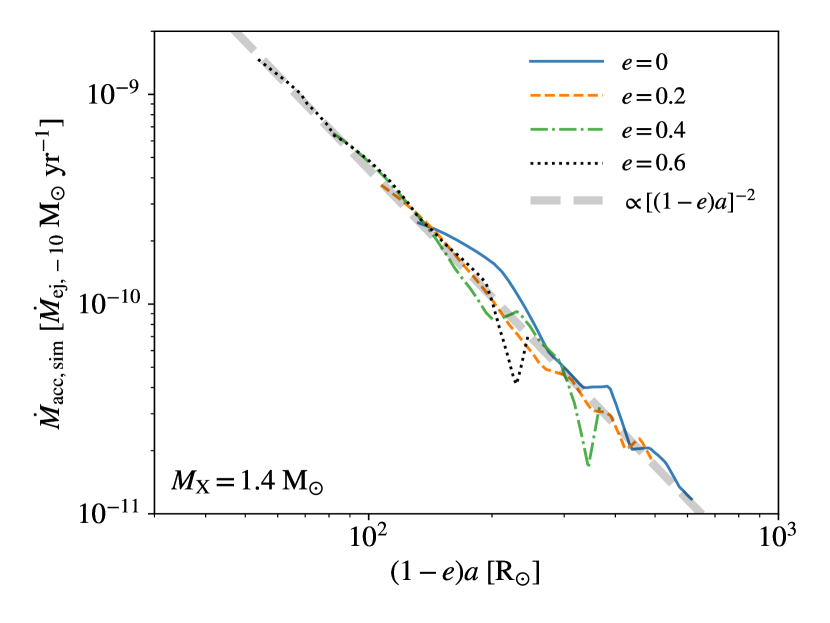
Figure 1: Relation between the peak accretion rate and pericenter distance based on the simulation results in Brown et al. (2019, see their fig. 7) for eccentricity $e=0$ (solid), 0.2 (thin dashed), 0.4 (dash-dotted) and 0.6 (dotted), in the unit of $\dot{M}_{\rm ej,-10}\ \rm M_{\odot}\ yr^{-1}$ given $\dot{M}_{\rm ej,-10}\equiv\dot{M}_{\rm ej}/(10^{-10}\ \rm M_{\odot}\ yr^{-1})$. The relation can be well described by a power-law $\dot{M}_{\rm acc,sim}\propto[(1-e)a]^{-2}$ as shown by the thick dashed line. These simulations consider a NS with $M_{\rm X}=1.4\ \rm M_{\odot}$ around a Be star of $M_{\star}=18\ \rm M_{\odot}$ and $R_{\star}=7\ \rm R_{\odot}$ with $\alpha=0.63$ for $P_{\rm orb}\sim 40-400\ \rm days$ and derive the median peak accretion rate from 5 orbits after the system settles to steady state.

In reality, mass ejection can be highly variable, even leading to disk dissipation/formation at timescales of a few years (Reig, 2011), and the viscosity parameter $\alpha$ can vary from system to system (Vieira et al., 2017; Rímulo et al., 2018), so that VDDs are more complex in reality than simulated by Brown et al. (2019) at steady state. Therefore, the accretion rate predicted by Eq. 9 should be regarded as an order-of-magnitude estimate that captures the increasing trend with decreasing pericenter distance $(1-e)a$. Finally, we multiply the peak accretion rate from Eq. 9 by a factor of $(R_{\rm trunc}/R_{\rm L1})^{8}$ for systems with $R_{\rm trunc}<R_{\rm L1}$ to capture the steepening of disk density profile beyond $R_{\rm trunc}$ (Okazaki et al., 2002).

Next, we associate the VDD base density $\Sigma_{0}$ with the donor star mass $M_{\star}$ by fitting observational data (Vieira et al., 2017; Rímulo et al., 2018). The obtained empirical scaling laws capture the increasing trend of $\Sigma_{0}$ with $M_{\star}$ (Arcos et al., 2017; Klement et al., 2017; Vieira et al., 2017; Rímulo et al., 2018), as shown in Fig. 2. To be specific, we have

$$\log(\tilde{\Sigma}_{0,\rm MW}\ [{\rm g\ cm^{-2}}])\simeq 1.44\log(M_{\star}\ [{\rm M_{\odot}}])-2.37$$ (10)

with $\simeq 0.52$ dex scatter by fitting the data of 80 Be stars observed in the MW (Vieira et al., 2017), and

$$\log(\tilde{\Sigma}_{0,\rm SMC}\ [{\rm g\ cm^{-2}}])\simeq 1.03\log(M_{\star}\ [{\rm M_{\odot}}])-0.99$$ (11)

of $\simeq 0.17$ dex scatter for 54 Be stars observed in the SMC (Rímulo et al., 2018). The observations by Rímulo et al. (2018) are likely biased towards dense disks, such that Eq. 11 should be regarded as an upper limit. Besides, to consider the large scatter in $\Sigma_{0}$ at similar $M_{\star}$, for each Be-XRB, we draw a random number $\chi$ from a Gaussian distribution of a standard deviation $\sigma=0.52\ (0.17)$ dex, and set $\Sigma_{0}=10^{\chi}\tilde{\Sigma}_{0,\rm MW\ (SMC)}(M_{\star})$, given the prediction of the best-fit model $\tilde{\Sigma}_{0,\rm MW\ (SMC)}(M_{\star})$ for the MW (SMC). In addition to the donor mass dependence, we also consider the metallicity $Z$ dependence of $\Sigma_{0}$ with two cases. In the conservative (CS) case, we always use the MW model independent of $Z$, motivated by the finding that the X-ray luminosity per luminous HMXB is insensitive to metallicity for $Z\sim 0.0004-0.03$ in nearby galaxies (Douna et al., 2015, see their fig. 5), while in the optimistic (OP) case, we assume that $\Sigma_{0}$ increases with decreasing metallicity with a linear relation between $\log(\Sigma_{0})$ and $Z$ from solar to SMC metallicities, i.e., $Z\sim 0.0035-0.0142$, and adopt the MW model for $Z>\rm Z_{\odot}=0.0142$ (Asplund et al., 2009) and the SMC model for $Z<Z_{\rm SMC}=0.0035$ (Davies et al., 2015).

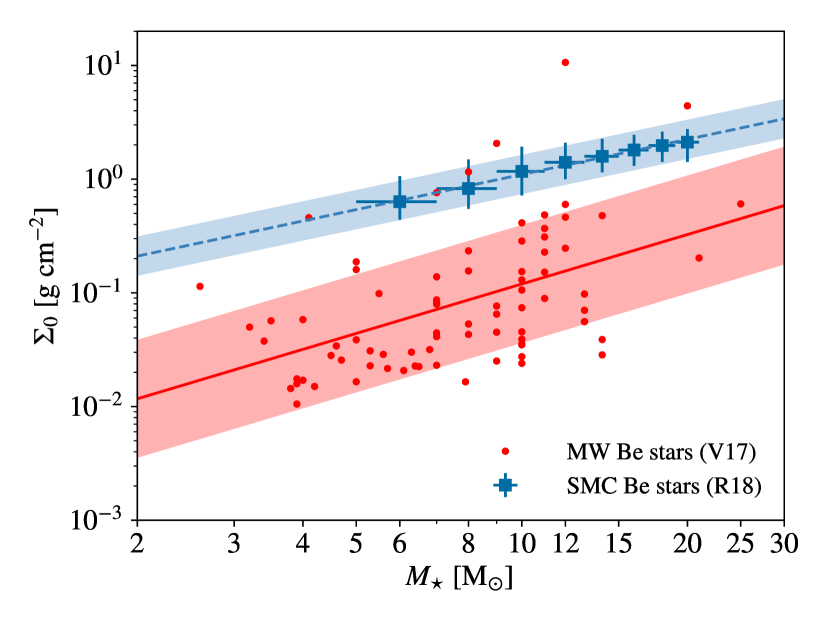
Figure 2: Relation between base disk surface density and Be star mass. The dots denote the 80 Be stars observed in the MW from Vieira et al. (2017, V17), which can be fit with a power-law relation $\log(\Sigma_{0}\ [{\rm g\ cm^{-2}}])\simeq 1.44\log(M_{\star}\ [{\rm M_{\odot}}])-2.37$ of $\simeq 0.52$ dex errors (shaded region around the solid line). The squares show the median base disk surface densities in 8 mass bins measured from 54 Be stars in the SMC (Rímulo et al., 2018, R18), where the errorbars show the bin size and 25-75% percentiles of $\Sigma_{0}$ in each bin. These results can also be described with a power-law $\log(\Sigma_{0}\ [{\rm g\ cm^{-2}}])\simeq 1.03\log(M_{\star}\ [{\rm M_{\odot}}])-0.99$ of $\simeq 0.17$ dex errors (shaded region around the dashed line).

To model the peak accretion rate and luminosity more precisely, we calibrate our model with observations of Be-XRBs in the MW. To do so, we apply the above formalism (at solar metallicity) to a randomly generated sample of 10000 NS-Be star binaries with a log-flat distribution of $a$ in the range of $[10-1000]\ \rm R_{\odot}$, a uniform distribution of eccentricity for $e\in[0,0.6]$ and a log-flat distribution of $M_{\star}$ for $M_{\star}\in[6,20]\ \rm M_{\odot}$, given fixed $M_{\rm X}=1.4\ \rm M_{\odot}$. From this sample we select a mock population of Be-XRBs with $P_{\rm orb}\sim 10-300\ \rm days$ and $L_{\rm X}>10^{34}\ \rm erg\ s^{-1}$ to be compared with observations. These conditions are chosen to mimic the statistics of most ($\sim 90$%) well observed Be-XRBs in the MW (Raguzova & Popov, 2005; Cheng et al., 2014; Brown et al., 2018). The calibration target is the relation between the (outburst) X-ray luminosity $L_{\rm X}$ and orbital periods $P_{\rm orb}$, derived by Dai et al. (2006, D06) based on 36 observed Be-XRBs from Raguzova & Popov (2005):

$$\log\left(\frac{L_{\rm X}}{10^{35}\rm\ erg\ s^{-1}}\right)$$

$$\quad\quad=4.53\pm 0.66-(1.50\pm 0.33)\log\left(\frac{P_{\rm orb}}{1\rm day}\right)\ .$$ (12)

The best-fit model indicates that the typical X-ray luminosity follows $L_{\rm X}\propto P_{\rm orb}^{-3/2}\propto a^{-9/4}$, which is similar to the $a$ dependence in $\dot{M}_{\rm acc,sim}\propto a^{-2}$. In light of this, we assume that $L_{\rm X}$ is proportional to the bolometric luminosity predicted by simulations with a calibration parameter $\psi_{\rm X}$: $L_{\rm X}=\psi_{\rm X}\epsilon\dot{M}_{\rm acc,sim}c^{2}$, given $\epsilon=0.2$ the typical radiative efficiency for NSs. This calibration factor captures the difference between X-ray luminosity and bolometric luminosity in observations as well as the difference between the peak accretion rates predicted by simulations and those in reality.

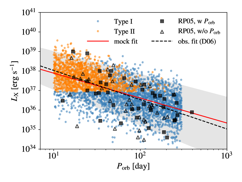
Figure 3: Relation between outburst X-ray luminosity and orbital period for the mock population of Be-XRBs with $P_{\rm orb}\sim 10-300\ \rm days$, $e\sim 0-0.6$ and $L_{\rm X}>10^{34}\ \rm erg\ s^{-1}$, given the calibration paremeter $\psi_{\rm X}=0.25$. Type I/II Be-XRBs are shown in blue/orange. These mock Be-XRBs are identified from 10000 randomly generated NS-Be star binaries with a log-flat distribution of separations for $a\in[10-1000]\ \rm R_{\odot}$, a uniform distribution of eccentricities for $e\in[0,0.6]$ and a log-flat distribution of Be star masses for $M_{\star}\in[6,20]\ \rm M_{\odot}$ given a fixed NS mass $M_{\rm X}=1.4\ \rm M_{\odot}$. We show the observed Be-XRBs compiled by Raguzova & Popov (2005, RP05, excluding V615 Cas and 2206+543) with filled squares and unfilled triangles. The filled squares have $P_{\rm orb}$ measured by observations, while for the unfilled triangles without $P_{\rm orb}$ measurements, we use the empirical scaling law $\log(P_{\rm orb}\ [{\rm day}])=0.4329\log(P_{\rm s}\ [{\rm s}])+1.043$ (Vinciguerra et al., 2020) to estimate $P_{\rm orb}$ given the spin period $P_{\rm s}$. The dashed line represents the best fit to observations from Dai et al. (2006) with the shaded region denoting the $1\sigma$ uncertainties in the fitting parameters (see Eq. 12). The solid line shows the best-fit power-law model for our mock population. It turns out that the mock population reproduces well observational data with a slightly shallower best fit and a similar scatter given $\psi_{\rm X}=0.25$.

If the observed X-ray luminosity completely dominates the bolometric luminosity and the simulations are realitic, we should have $\psi_{\rm X}\simeq 1$. However, we find that the empirical $L_{\rm X}$-$P_{\rm orb}$ scaling relation (Eq. 12) can be reproduced by the mock population with $\psi_{\rm X}=0.25\ll 1$, as shown in Fig. 3. There are two possible reasons for this low $\psi_{\rm X}$ value: (1) The accretion rates predicted by the simulations in Brown et al. (2019) are overestimated and/or the mass ejection rates of Be stars in Be-XRBs are lower than those of Be stars at large in the MW (Vieira et al., 2017). (2) The X-ray luminosity derived from observations in fact only represents a (small) fraction of the bolometric luminosity. To capture these uncertainties, we introduce a correction factor $f_{\rm corr}\in[\psi_{\rm X},1]$ (fixing $\psi_{\rm X}=0.25$) for the peak accretion rate $\dot{M}_{\rm acc}$. We also include a power-law term of $M_{\rm X}$ with index $\xi$ to account for the mass dependence, so that

$$\dot{M}_{\rm acc}=f_{\rm corr}\dot{M}_{\rm acc,sim}(a,e,\Sigma_{0})\left(\frac{M_{\rm X}}{1.4\ \rm M_{\odot}}\right)^{\xi} \ ,$$ (13)

where we adopt $\xi=2$ for Bondi-like accretion. Then the bolometric luminosity during outbursts of a Be-XRB can be written as

$$L_{\rm bol} =\epsilon\dot{M}_{\rm acc}c^{2}=f_{\rm corr}\times 5\times 10^{36}\ {\rm erg\ s^{-1}}$$

$$\times\left(\frac{\epsilon}{0.2}\right)\left[\frac{(1-e)a}{100\ \rm R_{\odot}}\right]^{-2}\left(\frac{\Sigma_{0}}{0.015\ \rm g\ cm^{-2}}\right)\left(\frac{M_{\rm X}}{1.4\ \rm M_{\odot}}\right)^{\xi}\ .$$ (14)

Here $f_{\rm corr}=1$ corresponds to the optimistic case in which the discrepancy is only caused by observational effects, while $f_{\rm corr}=0.25$ is the opposite end where the overestimation in simulations needs to be corrected the most. By default, we adopt $f_{\rm corr}=\psi_{\rm X}/f_{\rm BC,0}=0.5$, assuming a typical bolometric correction (BC) factor $f_{\rm BC,0}=L_{\rm X}/L_{\rm bol}=0.5$. The motivation is that most observations of Be-XRBs in Raguzova & Popov (2005) come from the $2-10$ keV band, which typically counts for $\sim 50$% of the bolometric luminosity (see Sec. 4 below).

Besides, we do not cape $\dot{M}_{\rm acc}$ at the Eddington rate

$$\dot{M}_{\mathrm{Edd}} \simeq 1.55\times 10^{-8}\ \mathrm{M_{\odot}\ yr^{-1}}\ \left(\frac{\epsilon}{0.2}\right)^{-1}\left(\frac{M_{\mathrm{X}}}{1.4\ \mathrm{M_{\odot}}}\right)\ ,$$ (15)

considering that Be-XRBs are promising candidates of ultra-luminous X-ray sources (ULXs, with $L_{\rm X}\gtrsim 10^{39}\ \rm erg\ s^{-1}$, reviewed by, e.g., Kaaret et al., 2017; Fabrika et al., 2021; King et al., 2023) and a few Be-XRBs with outburst luminosities above the Eddington luminosity $L_{\rm Edd}=\epsilon\dot{M}_{\rm Edd}c^{2}\sim 2\times 10^{38}\ \rm erg\ s^{-1}$ for typical NSs with $\epsilon=0.2$ and $M_{\rm X}=1.4\ \rm M_{\odot}$ have been observed (see table 1 of Karino 2022 and Fig. 3). Moreover, BPS studies show that XRBs (with both BH and NS accretors) can undergo episodes of highly super-Eddington (up to $\eta\sim 10^{3}$) mass transfer and potentially become ULXs (e.g., Marchant et al., 2017; Wiktorowicz et al., 2017, 2019, 2021; Shao et al., 2019; Shao & Li, 2020; Abdusalam et al., 2020; Kuranov et al., 2020; Misra et al., 2020). It is discussed below that ULXs are important in our Be-XRB populations.

We still use $L_{\rm bol}=\epsilon\dot{M}_{\rm acc}c^{2}$ when $\dot{M}_{\rm acc}>\dot{M}_{\rm Edd}$, ignoring any possible suppression of $L_{\rm bol}$ in the super-Eddington regime by, e.g., radiation-driven winds from the accretion disk (Shakura & Sunyaev, 1973), so that our results should be regarded as optimistic estimates. We also ignore the beaming effects of accretion disk geometry that can boost the apparent luminosities (and reduce the observed duty cycles or number counts) of ULXs with $\eta\equiv\dot{M}_{\rm acc}/\dot{M}_{\rm Edd}\gtrsim 8.5$ (King et al., 2001; King, 2009; Lasota & King, 2023). Our simple approach is motivated by the lack of features around the Eddington limits of NSs and BHs in the observed luminosity function of HMXBs, which implies that super-Eddington systems are most likely ‘normal’ XRBs similar to their sub-Eddington counterparts (Gilfanov et al., 2022).

3.2.2 Classification of X-ray outbursts & duty cycle

Now we can calculate the outburst strength by Eqs. 13 and 14. We further classify the outbursts into two categories following the convention in observations to estimate the duty cycle (Reig, 2011; Rivinius et al., 2013):

1. Type I outbursts are regular, (quasi-)periodic and short-lived ($\sim 0.1-0.3\ P_{\rm orb}$) increases of X-ray flux by a factor of $\sim 10-100$, peaking at or close to the pericentric passage of the compact object with X-ray luminosities $L_{\rm X}\lesssim 10^{37}\ \rm erg\ s^{-1}$. The duty cycle is typically $f_{\rm duty,I}\sim 0.1-0.3$ (Reig, 2011; Sidoli & Paizis, 2018).

2. Type II outbursts are major enhancements of X-ray flux, by a factor of $10^{3}-10^{4}$, even reaching the Eddington limit. They do not have preferred orbital phases and last longer than Type I outbursts (up to a few orbital periods). During a Type II outburst, a radiatively efficient thin accretion disk is expected to form around the compact object, and the VDD structure can be significantly disrupted. The duty cycle is usually lower than the Type I case: $f_{\rm duty,II}\sim 10^{-3}-0.1$ (Sidoli & Paizis, 2018; Xu & Li, 2019).

These two types of outbursts generally correlate with the two peaks in the observed bi-model spin period distribution of NSs in Be-XRBs, which can be divided by a critical spin period $P_{\rm s,crit}=40\ \rm s$ (Cheng et al., 2014; Haberl & Sturm, 2016; Xu & Li, 2019). To explain this correlation, it is proposed by Okazaki et al. (2013) with considerations of accretion timescale and spin-up efficiency that the two types of outbursts experience different modes of accretion: During a Type II outburst, the NS accretes at a high rate via a radiatively efficient thin accretion disk and is spun up efficiently to have spin periods $P_{\rm s}\lesssim 40\ \rm s$. In Type I outbursts, accretion is in the form of advection dominated accretion flow (ADAF) resulting in low spins with $P_{\rm s}\gtrsim 40\ \rm s$. It is further shown by Cheng et al. (2014) that disk warping plays an important role in the spin evolution of NSs, such that Type II outbursts tend to occur when NSs interact with tidally warped VDDs. Motivated by these results (and generalizing them to BHs), we assume that a Be-XRB will have Type II outbursts when two criteria for (1) tidal warping and (2) accretion rate are satisfied, as defined below.

1. Following the analysis in Cheng et al. (2014) for the power-law+Gaussian VDD model (see sec. 2.2 of Martin et al., 2011), the tidal warping criterion is satisfied when the disk truncation radius at periastron $R_{\rm trunc,p}=f_{\rm trunc}(1-e)a$ is larger than the tidal warping radius (eq. 30 in Martin et al., 2011):

   $$R_{\rm tid} =\left[\frac{2\nu_{\star}(GM_{\star})^{1/2}\bar{R}_{\rm b}^{3}}{3GM_{\rm X}R_{\star}^{n-2}}\right]^{\gamma}$$

   $$=a^{3\gamma}(1-e^{2})^{3\gamma/2}\left[\frac{2\alpha H_{\star}^{2}M_{\star}}{3M_{\rm X}R_{\star}^{n-1/2}}\right]^{\gamma}\ ,$$ (16)

   where $\nu_{\star}=\alpha H_{\star}^{2}R_{\star}^{3/2}(GM_{\star})^{1/2}$ is the (base) disk viscosity at the stellar surface, $\bar{R}_{\rm d}=a(1-e^{2})^{1/2}$ is the average separation, $H_{\star}=\sqrt{2}c_{s}v_{\rm Kep}^{-1}R_{\star}$ ($\simeq 0.04R_{\star}$, Wood et al., 1997) is the (base) scale height of the disk at the stellar surface (Klement et al., 2017), and the power-law index $\gamma=2/(11-2n)\sim 0.5$ is given by $n\sim 3.5$ which is the slope of the disk (mid-plane) density profile (see eqs. 12, 16 and 29 in Martin et al., 2011). Substituting the formula of $R_{\rm tid}$ (Eq. 16) to the iniquity $f_{\rm trunc}a(1-e)>R_{\rm tid}$, we have

   $$a<a_{\rm crit}\equiv\left[\frac{f_{\rm trunc}(1-e)}{(1-e^{2})^{\frac{3\gamma}{2}}}\left(\frac{3}{2\alpha}\frac{M_{\rm X}}{M_{\star}}\frac{R_{\star}^{n-1/2}}{H_{\star}^{2}}\right)^{\gamma}\right]^{\frac{1}{{(3\gamma-1)}}}\ ,$$ (17)

   in which $f_{\rm trunc}$ is given by Eq. 7. Here we use $\alpha=0.63$ to evaluate the critical seperation $a_{\rm crit}\propto\alpha^{-\gamma/(3\gamma-1)}\sim\alpha^{-1}$ in Eq. 17, motivated by the finding in Cheng et al. (2014) that the observed populations of Be-XRBs with low ($P_{\rm s}>40$ s) and high ($P_{\rm s}<40$ s) spins, roughly corresponding to Type I and II outbursts, can be well divided by the tidal warping criterion with $\alpha\sim 0.5-1$. However, the adopted value of $\alpha$ here is much lower than the viscosity parameter for vertical shear $\alpha_{2}=2.66$ considered in Martin et al. (2011). It is shown below that our choice of $\alpha$ is justified by comparing the mock population of Be-XRBs with observations (Fig. 4). The discrepancy here may be caused by the fact that the VDD flares (reaching $H/R\gtrsim 0.1$ at $R\gtrsim 10R_{\star}\sim 100\ \rm R_{\odot}$) while the value in Martin et al. (2011) is derived for thin ($H/R\ll 1$), flat disks (Ogilvie, 1999; Lodato & Price, 2010). The disk flaring may reduce the viscosity for vertical shear and enhance vertical diffusion, making the disk more vulnerable for tidal warping (with $R_{\rm tid}$ smaller by a factor of $\sim 2$).

2. The accretion rate criterion can be written as

   $$\eta\equiv\dot{M}_{\rm acc}/\dot{M}_{\rm Edd}>\eta_{\rm crit}\ .$$ (18)

   Here we adopt the typical radiative efficiencies $\epsilon=0.2$ for NSs and $\epsilon=0.1$ for BHs to calculate the Eddington rate $\dot{M}_{\rm Edd}$ (Eq. 15). We expect the transition Eddington ratio to be in the range $\eta_{\rm crit}\sim 0.05-0.2$, where the upper limit is adopted in Okazaki et al. (2013) to explain the outburst strengths of Type I and II in simulations, while the lower limit is consistent with the theoretical thin disk formation criterion $\eta>0.07\alpha$ adopted in Takhistov et al. (2022) based on Pringle (1981), given the viscosity parameter $\alpha=0.63$ in our case. We set $\eta_{\rm crit}=0.2f_{\rm corr}$, because with this choice the $L_{\rm X}$ distributions of Type I and II outbursts from the mock population are generally consistent with those of observed Be-XRBs corresponding to the two peaks of spin period distribution at $P_{\rm s}>40$ s and $P_{\rm s}<40$ s (see, e.g., fig. 3 in Cheng et al., 2014), as shown in Fig. 4. Since our mock population of Be-XRBs is not meant to fully capture the statistics of observed Be-XRBs complied by Cheng et al. (2014), it does not reproduce the quasi-bi-modal feature of the observed $L_{\rm X}$ distribution.

Given the above classification, we combine the optimistic duty cycles $\hat{f}_{\rm duty}$ in observations of the two types of outbursts, $\hat{f}_{\rm duty,I}=0.3$ and $\hat{f}_{\rm duty,II}=0.1$, with a physical limit $f_{\rm duty,\max}=\dot{M}_{\rm ej}/\dot{M}_{\rm acc}$ to estimate the (average) duty cycle as $f_{\rm duty}=\min(\hat{f}_{\rm duty},f_{\rm duty,max})$ where

$$\dot{M}_{\rm ej} =f_{\rm corr}\times 10^{-10}\ {\rm M_{\odot}\ yr^{-1}}(\Sigma_{0}/0.015\ \rm g\ cm^{-2})\ ,$$ (19)

is the mass ejection rate for $\alpha=0.63$ based on the results from Brown et al. (2019). The limit $f_{\rm duty,\max}$ captures the simple requirement that the compact object does not accrete more than what is ejected from the O/B star. When $f_{\rm duty,\max}<\hat{f}_{\rm duty}$, we assume that the compact object is able to accrete all materials ejected by the O/B star during X-ray outbursts, despite the fact that for classical O/Be stars only a small fraction ($\sim 0.01$) of the ejected materials is expected to settle into the disk according to the standard steady-state VDD model (e.g., Haubois et al., 2012; Rímulo et al., 2018), while the majority will fall back to the star. This optimistic assumption is required to explain the observed high duty cycles (up to $0.3$, Reig, 2011; Sidoli & Paizis, 2018). It means that mass replenishment of VDDs is much more efficient for O/Be stars in Be-XRBs than predicted by the standard VDD model (for O/Be stars in isolation), which is supported by the shorter disk timescales of Be stars in Be-XRBs compared with single Be stars in observations (Reig, 2011).

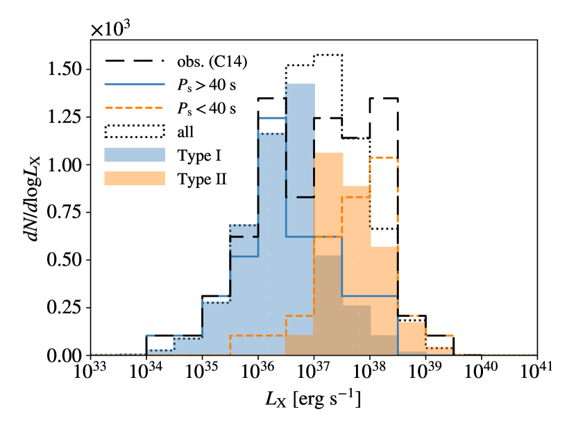
Figure 4: Distribution of outburst X-ray luminosity for the mock population of Be-XRBs (dotted contour, see Fig. 3) in comparison with that of the 71 observed Be-XRBs (long-dashed contour) complied by Cheng et al. (2014, C14, see their fig. 3). The observed distribution is re-normalized to have the same total number of Be-XRBs. For the mock population, contributions from Type I and II outbursts are plotted with the right and left shaded histograms in blue and orange, respectively, while for the observed population, the sub groups of X-ray pulsars with spin periods $P_{\rm s}$ above and below 40 seconds are shown with the solid and dashed contours. The $L_{\rm X}$ distribution and fraction of Type I (II) events from our mock population are generally consistent with those of the observed Be-XRBs with $P_{\rm s}>\ (<)\ 40\ \rm s$.

With this model, we find that most Be-XRBs in the mock population do satisfy $f_{\rm duty,I}\sim 0.1-0.3$ and $f_{\rm duty,II}\sim 0.01-0.1$, which is generally consistent with observations (Reig, 2011; Sidoli & Paizis, 2018; Xu & Li, 2019). In the mock population, evolution of binary and stellar parameters during the Be-XRB phase is ignored, whereas in the BPS runs such evolution can change the outburst type of a Be-XRB. Be-XRBs with both types of outbursts also exist in observations. We classify the systems that experience both types of outbursts as Type I/II. Besides, when $\dot{M}_{\rm acc}$ is comparable to $\hat{f}_{\rm duty}^{-1}\dot{M}_{\rm ej}$ (such that $f_{\rm duty}\lesssim\hat{f}_{\rm duty}$), significant disruption of the VDD by the compact object is expected to happen, such that the system will show Type II features especially with low $f_{\rm duty}$. Therefore, we also regard the Be-XRBs classified as Type I according to Eqs. 17 and 18 with $f_{\rm duty}<0.1$ as Type I/II in post-processing. Finally, we count Type I/II systems into the general Type II category, which refers to all Be-XRBs that once undergo major outbursts with high accretion rates, disk warping and/or disruption. Recent observations find that the outburst behaviors of Be-XRBs are likely more diverse and complex than the conventional two types (Sidoli & Paizis, 2018). Nevertheless, our consideration of the outburst type only affects the final X-ray output indirectly by the optimistic duty cycle $\hat{f}_{\rm duty}$, and we have verified by numerical experiments that our results are insensitive to outburst classification. The reason is that the majority ($\sim 60-70$%) of X-ray emission comes from systems with $f_{\rm duty}\simeq f_{\rm duty,max}\lesssim\hat{f}_{\rm duty}$ in all Be-XRB populations considered here.

4 X-ray spectral model

Once $L_{\rm bol}$ is known, we only need to determine the spectral shape to obtain the full (intrinsic) spectral energy distribution (SED) of X-ray outbursts. For simplicity, we consider three regimes of accretion rates: low-hard (LH, $\eta<0.05$), high-soft (HS, $\eta\sim 0.05-2$) and super-Eddington (SE, $\eta>2$), for both NSs and BHs. Motivated by the ideas in Fragos et al. (2013a), we find the typical spectral shape in each regime by fitting simple spectral models to the BC factors measured in observations (e.g., McClintock & Remillard, 2006; Wu et al., 2010; Anastasopoulou et al., 2022) for select energy bands. Here we consider the photon energy range $E\sim 10^{-4}-10^{4}$ keV assuming that this contains most of the power.

We take the recent measurements of BC factors of the energy bands $E\sim 0.5-2$, $2-10$ and $12-15$ keV by Anastasopoulou et al. (2022, see their table 4, A1, A6, A9 and A10) for both NS and BH HMXBs as references. We estimate the typical value (and uncertainty) of the BC factor for each band in each regime, as shown in Fig. 5. These estimates are used to construct reference spectral energy distributions (SEDs) that serve as the targets of spectral fitting. Since soft X-ray photons in the $E\sim 0.5-2$ keV band are mostly responsible for X-ray heating of the IGM (Das et al., 2017), we increase the weight of this band by a factor of 4 in the fitting process to better reproduce the corresponding BC factor.

For simplicity, we assume that for both NSs and BHs the final spectrum is made of two components: an input spectrum and a spectrum of inverse Compton scattered photons (by corona electrons) with a power-law tail in the high-energy end. Following Sartorio et al. (2023), we use the SIMPL-1 Comptonizon model in Steiner et al. (2009, see their eqs. 1 and 4) to connect the up-scattered component with the input spectrum $L_{\nu,\rm in}$ via two parameters: the fraction $f_{\rm scatter}$ of photons in the input (photon number) spectrum $n_{\rm in}(E)\equiv dN_{\rm in}/dE=(hE)^{-1}L_{\nu,\rm in}$ that are up scattered, and the power-law index $\Gamma$ in the spectrum of up-scattered photons:

$$n_{\rm out}(E) =(1-f_{\rm scatter})n_{\rm in}(E)$$

$$+f_{\rm scatter}\int_{E_{\min}}^{E}n_{\rm in}(E_{0})G(E,E_{0})dE_{0}\ ,$$ (20)

where $G(E,E_{0})=(\Gamma-1)(E/E_{0})^{-\Gamma}/E_{0}$ is the Green’s function of inverse Compton scattering. The final specific luminosity can then be derived from the output photon number spectrum with $n_{\rm out}(E)\equiv dN_{\rm in}/dE=(hE)^{-1}L_{\nu,\rm out}$.

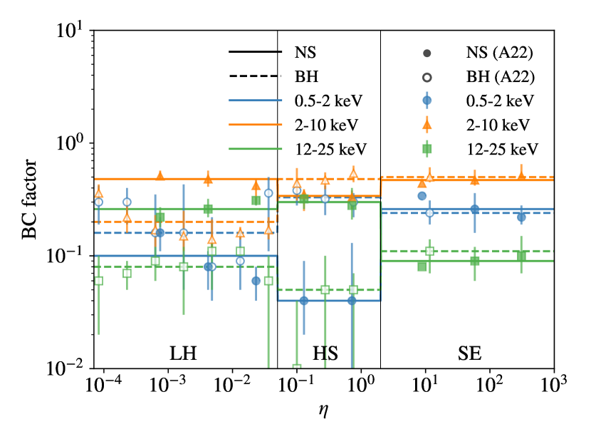
Figure 5: BC factor as a function of Eddington ratio $\eta$. The solid and dashed lines show the values adopted in our spectral fitting process for NSs ($M_{\rm X}\leq 2.2\ \rm M_{\odot}$) and BHs ($M_{\rm X}>2.2\ \rm M_{\odot}$), respectively, considering the energy bands $E\sim 0.5-2$ keV (blue), $2-10$ keV (orange), and $12-25$ keV (green), based on the measurements in Anastasopoulou et al. (2022, A22, see their table 4, A1, A6, A9 and A10). For comparison, we also show their original data for $E\sim 0.5-2$ keV (circles), $2-10$ keV (triangles), and $12-25$ keV (squares), where the results for NSs and BHs are denoted by filled and unfilled data points, respectively.

For the input spectrum, we adopt the black body (BB) spectrum for NSs assuming that the majority of X-ray radiation is produced at hot spots on the NS surface from inflows channeled by magnetic fields. The top row of Fig. 6 shows the resulting best-fit spectral models in the three regimes with $k_{\rm B}T\sim 0.4-0.9$ keV, $f_{\rm scatter}\sim 1$ and $\Gamma\sim 2.5-2.7$.

While for BHs, we use the thin disk (TD) model (Pringle, 1981; Takhistov et al., 2022)

$$L_{\nu,\rm TD}\propto\begin{cases}\left(\frac{T_{\max}}{T_{\rm o}}\right)^{5/3}\left(\frac{\nu}{\nu_{\max}}\right)^{2}\ ,\quad h\nu\leq k_{\rm B}T_{\rm o}\ ,\\ (\nu/\nu_{\max})^{1/3}\ ,\quad k_{\rm B}T_{\rm o}<h\nu<k_{\rm B}T_{\max}\ ,\\ \left(\frac{\nu}{\nu_{\max}}\right)^{2}\exp\left(1-\frac{\nu}{\nu_{\max}}\right)\ ,\ h\nu>k_{\rm B}T_{\max}\ ,\end{cases}$$ (21)

where $T_{\max}=0.488T_{i}$, $T_{\rm o}\simeq T_{\rm i}(R_{\rm i}/R_{\rm o})^{3/4}$ and $\nu_{\max}=k_{\rm B}T_{\max}/h$, given $T_{\rm i}$ as the temperature at the inner edge ($R_{\rm i}=6GM_{\rm X}/c^{2}$) of the TD, and $T_{\rm o}$ as the temperature at the outer disk boundary $R_{\rm o}\sim R_{\rm L1}(a,e,q_{\rm X})$. Since very close binaries ($P_{\rm orb}\lesssim 7$ days) and RLO are forbidden for Be-XRBs (Panoglou et al., 2016; Panoglou et al., 2018; Rivinius, 2019) by tidal forces that can slow down the rotation of donor stars, we have $R_{\rm o}\gtrsim 2\ \rm R_{\odot}$ and $k_{\rm B}T_{\rm o}\lesssim 10^{-3}$ keV in most cases. Therefore $R_{\rm o}$ is unimportant for X-rays that we are concerned with ($E>0.1$ keV) and the input TD spectrum is controlled by a single parameter $T_{\rm i}$ during the fitting process. The best-fit models for $M_{\rm X}=4\ \rm M_{\odot}$ and $R_{\rm o}=10\ \rm R_{\odot}$ are shown in the bottom row of Fig. 6 with $k_{\rm B}T_{\rm i}\sim 0.7-1.5$ keV, $f_{\rm scatter}\sim 0.3-1$ and $\Gamma\sim 2.1-2.8$.

(a)

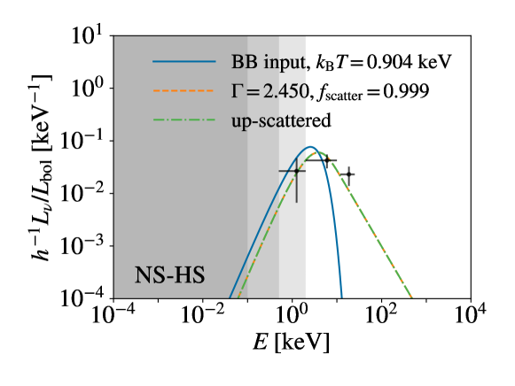
(b)

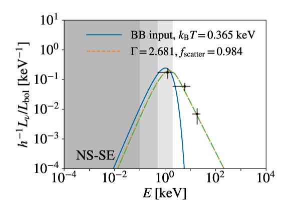
(c)

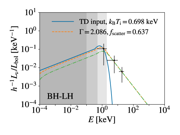
(d)

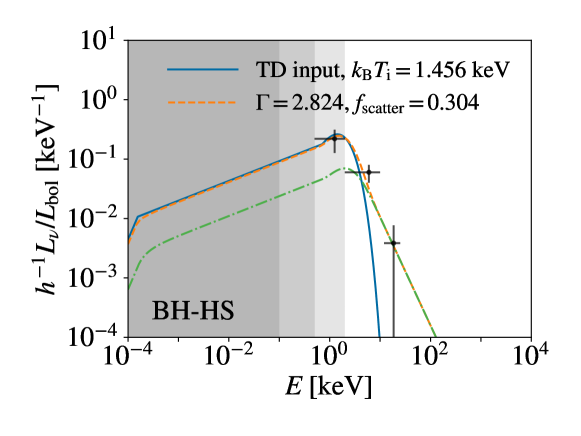
(e)

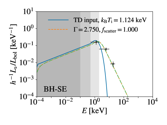
(f)

Figure 6: Best-fit spectral models for NSs (top) and BHs (bottom) in the low-hard (LH, $\eta<0.05$, left), high-soft (HS, $\eta\sim 0.05-2$, middle) and super-Eddington (SE, $\eta>2$, right) regimes, in terms of $L_{\nu}/(hL_{\rm bol})$. Here we assume $M_{\rm X}=4\ \rm M_{\odot}$ and $R_{\rm o}=10\ \rm R_{\odot}$ for the BH spectra. In each case the input spectrum is shown with the solid curve, the final spectrum with the dashed curve and the up-scattered component with the dash-dotted curve, respectively. The data points with error bars show the reference SEDs inferred from the BC factor measurements in Anastasopoulou et al. (2022). The dark ($E\lesssim 0.1\ \rm keV$), intermediate dark ($E\lesssim 0.5\ \rm keV$) and light ($E\sim 0.5-2\ \rm keV$) shaded regions denote the parts of the spectrum that are expected to be absorbed by the ISM in typical high-$z$ HMXB-hosting minihaloes (Sartorio et al., 2023), atomic cooling haloes (Das et al., 2017), and the IGM at $z\sim 15$ (Pritchard & Furlanetto, 2007).

5 Results

Combining the two choices for initial rotation parameter $W_{0}$: SR or FR (Sec. 2.3), and the two models for VDD density $\Sigma_{0}$: CS or OP (Sec. 3.2), we have 4 models to explore, which are summarized in Table 2. For each model, we consider ten cases at $Z=10^{-4}$, $3\times 10^{-4}$ $10^{-3}$, 0.0035, 0.005, 0.007, 0.01, 0.0142, 0.02 and 0.03, where $Z=0.0035$, 0.07 and 0.0142 correspond to the situations of the SMC, LMC and MW, respectively. Since the CS and OP models are identical at $Z\geq 0.0142$, we only need to run 34 BPS simulations in total. We record the time-averaged values of the Be-XRB properties including properties of donors and accretors, orbital parameters as well as X-ray outburst properties, which are then used to calculate the total X-ray output. Considering the short lifetimes of Be-XRBs, for simplicity, when calculating the total X-ray emission of a Be-XRB population, we assume no variation of X-ray outburst properties during the Be-XRB phase, which is a simplification of the reality that VDDs can be highly variable structures with disk dissipation/formation at timescales of a few years (Reig, 2011; Rivinius et al., 2013). Since our purpose is to evaluate the overall X-ray output from a population of Be-XRBs, higher-order effects are expected to be unimportant. In this section we mainly show the results from the SR_CS model with $f_{\rm corr}=0.5$, defined as the fiducial case, because it achieves the best agreement with observations and the key trends in the metallicity dependence of Be-XRB properties are similar in the other cases. Select results for the other 3 models in Table 2 and different values of $f_{\rm corr}$ are included in Appendix B.

Table 2: Summary of models. The second column shows the choices of the initial rotation parameter $W_{0}\equiv v_{\rm rot,0}/v_{\rm Kep,0}$ given the initial rotation velocity $v_{\rm rot,0}$ and Keplerian velocity $v_{\rm Kep,0}$ at the stellar equator (see Sec. 2.3), where the slowly-rotating (SR) model $W_{0}(M_{\star},Z)$ with mass and metallicity dependence is based on Hurley et al. (2000, see their sec. 7.2) and Hurley et al. (2002), while the fast-rotating (FR) model uses a constant high value. The third column shows the choices of the (base) surface density $\Sigma_{0}$ of decretion disk (see Sec. 3.2), where the metallicity-dependent optimistic (OP) model uses a linear interpolation for $\log(\Sigma_{0})$ between the MW fit for at $Z=0.0142$ (Eq. 10) and the SMC fit at $Z=0.0035$ (Eq. 11), while the conservative model adopts the MW fit at all metallicities.

Model	$W_{0}$	$\Sigma_{0}$
SR_CS	$W_{0}(M_{\star},Z)$	$\Sigma_{0}(M_{\star})$ (Eq. 10)
FR_CS	0.9	$\Sigma_{0}(M_{\star})$ (Eq. 10)
SR_OP	$W_{0}(M_{\star},Z)$	$\Sigma_{0}(M_{\star},Z)$ (Eqs. 10 and 11)
FR_OP	0.9	$\Sigma_{0}(M_{\star},Z)$ (Eqs. 10 and 11)

5.1 Formation efficiency

We first look into the formation efficiency of active Be-XRBs, $\mathcal{N}_{\rm X}$, as a function of $Z$ which, considering the short lifetimes (a few to a few tens Myr) of Be-XRBs, is defined as the number of Be-XRBs in the outburst phase per unit SFR for a long enough star formation timescale ($\tau_{\rm SF}\gtrsim 100$ Myr). Given $N$ Be-XRBs predicted by a BPS run for a single-age stellar population of a total mass $M_{\rm tot}$, the formation efficiency can be written as

$$\mathcal{N}_{\rm X} \equiv\frac{\langle N_{\rm X}\rangle}{{\rm SFR}}=\frac{1}{{\rm SFR}}\sum_{i}^{N}f_{{\rm duty},i}\left(\frac{\tau_{i}{\rm SFR}}{M_{\rm tot}}\right)=\sum_{i}^{N}\frac{f_{{\rm duty},i}\tau_{i}}{M_{\rm tot}}\ ,$$ (22)

where $\tau_{i}$ is the duration of the Be-XRB phase for binary $i$.

The results for all the 4 models in Table 2 are shown in Fig. 7, where we count both the number of all Be-XRBs (thin curves with markers) and that of Be-XRBs with $e>0.1$ (thick curves without markers). The latter case is meant to capture the situation assumed in previous BPS studies of Be-XRBs (e.g., Zhang et al., 2004; Xing & Li, 2021) that tidal truncation of the VDD is sharp, leading to a smaller disk boundary at $R_{\rm trunc}$ (Eq. 7) than the one adopted in our model ($R_{\rm crit}$, see Eq. 8). In both cases, $\mathcal{N}_{\rm X}$ generally increases with decreasing $Z$, but the evolution is not fully monotonic for all Be-XRBs, which has a small peak at $Z=0.005$ and a small dip at $Z=0.01$. The general trend is driven by the stronger stellar winds at higher $Z$ that increasingly widen binary orbits and reduce the number of stars that can become NSs and BHs. The non-monotonic features are likely caused by the complex interplay between stellar winds and mass transfer rate (see Sec. 5.2). We also find that nearly-circular ($e\leq 0.1$) systems make up a significant fraction ($\sim 40-80\%$) of active Be-XRBs at $Z\lesssim 0.02$. Naïvely, this seems in tension with the rareness ($\lesssim 10\%$) of such Be-XRBs in observations (Cheng et al., 2014; Sidoli & Paizis, 2018). However, observations are very likely incomplete at the low eccentricity end because the measurement of $e$ is difficult for nearly-circular binaries, and only a small fraction of observed Be-XRBs have eccentricity measurements. Besides, these binaries are typically faint with $L_{\rm bol}\sim 10^{33}-10^{37}\ \rm erg\ s^{-1}$ due to the suppressed accretion rate from disk truncation, and therefore, difficult to detect. In fact, they produce much less X-rays compared with their more eccentric counterparts such that ignoring them has little (up to a few percent) impact on the overall X-ray output.

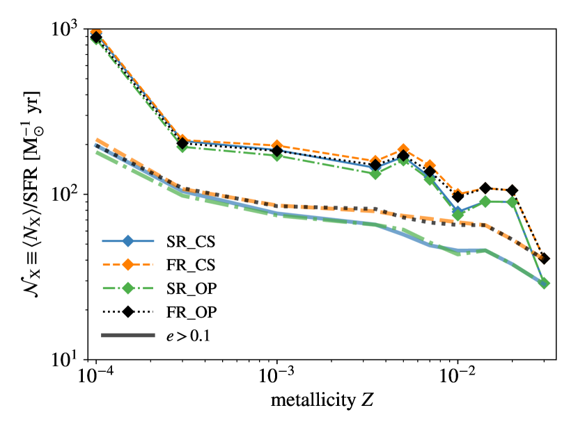
Figure 7: Number of Be-XRBs (in the outburst phase) per unit SFR as a function of metallicity, for the SR_CS (solid), FR_CS (dashed), SR_OP (dash-dotted) and FR_OP (dotted) models. The results for all Be-XRBs are shown with the thin curves marked by diamonds, while the unmarked thick curves show the results for Be-XRBs with $e>0.1$. The thin vertical lines label the metallicities of the MW, LMC and SMC (from right to left).

Last but not the least, $\mathcal{N}_{\rm X}$ is higher in the FR models with higher initial rotation rates than in the SR models as expected. The difference between the FR and SR models is larger at higher $Z$ but remains below $\sim 40\%$ and becomes even comparable to the uncertainties in $\mathcal{N}_{\rm X}$ at $Z\lesssim 0.0035$. The overall small difference indicates that in most binaries that can potentially become Be-XRBs the (initial) secondary star will be spun up to become an O/Be star (via stable mass transfer during the MS and HG phases) regardless of its initial rotation rate. This is consistent with the scenario that all or most (young) O/Be stars are produced by mass and angular momentum transfer from companion stars (Shao & Li, 2014; Hastings et al., 2020; Hastings et al., 2021; Dodd et al., 2023; Wang et al., 2023), which is supported by observations that find a large fraction of classical Be stars with disk truncation (i.e., SED turndown; Klement et al., 2019), the lack of close Be binaries with MS companions (Bodensteiner et al., 2020), and a higher run-away/field frequency of O/Be stars (or fast rotators) compared with normal O/B stars (Dorigo Jones et al., 2020; Dallas et al., 2022). On the other hand, the difference between the FR and SR models is generally larger when we focus on Be-XRBs with $e>0.1$ at $Z\gtrsim 10^{-3}$. The reason is that mass transfer is weaker in these systems leading to less efficient spin-up of the secondary star, as discussed below (Sec. 5.2). Besides, the difference is smaller at lower $Z$, where the secondary stars are more compact and are more easily spun up to become O/Be stars.

Figure 8: Number of (ultra-)luminous Be-XRBs (in outbursts) per unit SFR as a function of metallicity in the SR_CS model with $f_{\rm corr}=0.5$. The BPS results for luminous ($L_{[0.5-8]~{}\rm keV}>10^{38}\ \rm erg\ s^{-1}$) and ultra-luminous ($L_{[0.5-8]~{}\rm keV}>10^{39}\ \rm erg\ s^{-1}$) sources are shown by the dashed and solid curves, respectively. For comparison, we show the observational data from Douna et al. (2015, D15, see their fig. 4) for $L_{[0.5-8]~{}\rm keV}>10^{38}\ \rm erg\ s^{-1}$ with the crosses, and those from Kovlakas et al. (2020, K20, see their fig. 14) for $L_{[0.5-8]~{}\rm keV}>10^{39}\ \rm erg\ s^{-1}$ with circles, which include the data originally from Mapelli et al. (2010). The uncertainties in these data are typically large ($\sim 0.5$ dex), as implied by their scatter around similar metallicities. The number counts for ultra-luminous sources ($L_{[0.5-8]~{}\rm keV}>10^{39}\ \rm erg\ s^{-1}$) from the observed HMXB sample in Lehmer et al. (2021, L21, see their table 3 and fig. 6) are denoted by the squares with ($1\sigma$) error bars, and the shaded region denotes the 16-84% confidence range obtained with mock populations of XRBs sampled from their best-fit model for $Z$-dependent X-ray luminosity functions. The thin vertical lines label the metallicities of the MW, LMC and SMC (from right to left).

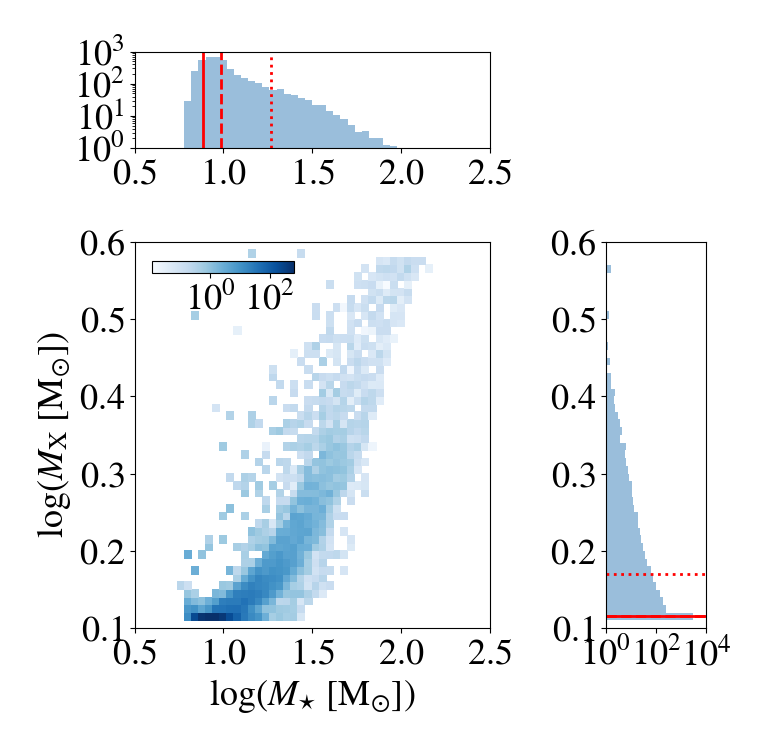
(a) $Z=10^{-4}$

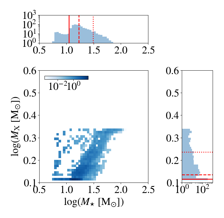
(b) $Z=0.0035$ (SMC)

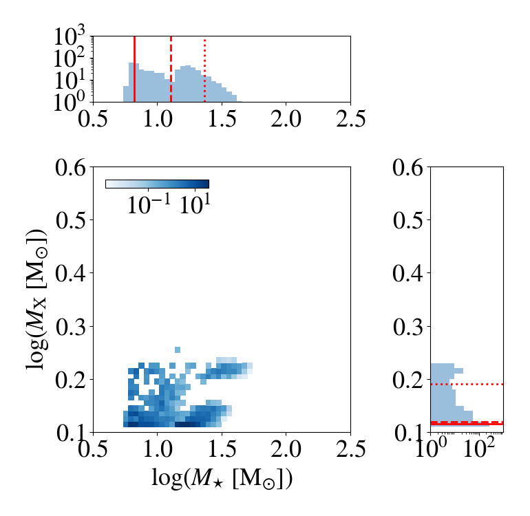
(c) $Z=0.0142$ (MW)

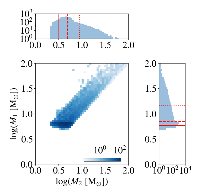
(d)

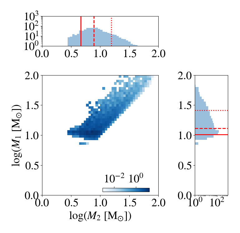
(e)

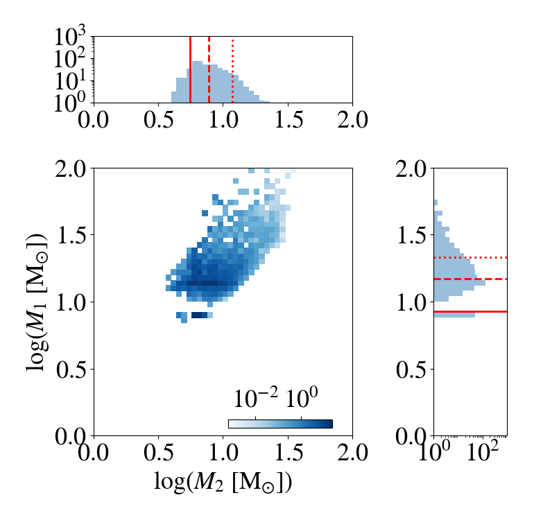
(f)

(g)

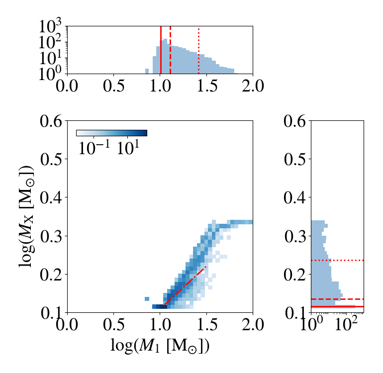
(h)

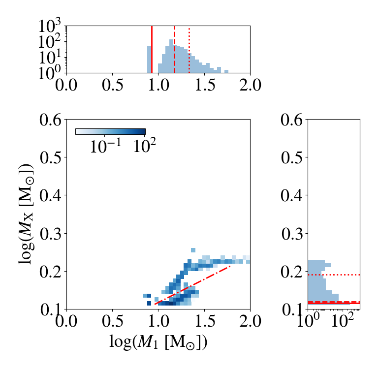
(i)

Figure 9: Mass distributions of Be-XRBs (top) and their progenitors (middle), and the initial-remnant mass relation for primary stars of Be-XRB progenitors (bottom) in the SR_CS model for $Z=10^{-4}$ (left), $Z=0.0035$ (middle) and $Z=0.0142$ (right). Here the (initial) primary star ($M_{1}$) is the progenitor of the compact object ($M_{\rm X}$), and the (initial) secondary star ($M_{2}$) is the progenitor of the O/Be star ($M_{\star}$). Each Be-XRB $i$ is weighted by $\tau_{i}/M_{\rm tot}$, so that the number for each bin on these plots corresponds to the expected number of binaries in the Be-XRB phase per unit SFR ($\rm M_{\odot}\ yr^{-1}$). In the marginalized distributions, the solid, dashed and dotted lines mark the 10, 50 and 90 percentiles. The dash-dotted lines in the 2D maps of initial-remnant mass relation for primary stars (bottom) approximately divide the Be-XRB population into two groups with lower and higher $M_{\rm X}$ in which the primary stars experience different levels of mass loss (see the main text in Sec. 5.2).

In addition to the general Be-XRB population, we also derive the number of luminous and ultra-luminous sources with broad-band ($E\sim 0.5-8$ keV) X-ray luminosities $L_{[0.5-8]~{}\rm keV}>10^{38}\ \rm erg\ s^{-1}$ and $L_{[0.5-8]~{}\rm keV}>10^{39}\ \rm erg\ s^{-1}$ during outbursts, respectively, for which constraints from observations of HMXBs in nearby galaxies are available down to $Z\sim 0.0003$ (Mapelli et al., 2010; Douna et al., 2015; Kovlakas et al., 2020; Lehmer et al., 2021). The results in our fiducial case are shown in Fig. 8. For utra-luminous sources with $L_{[0.5-8]~{}\rm keV}>10^{39}\ \rm erg\ s^{-1}$, we find that the numbers of Be-XRBs predicted by our BPS runs are lower than those inferred from observations of all types of HMXBs (Lehmer et al., 2021) by about 40% at $Z\sim 0.0003-0.02$, which means that the simulated Be-XRBs can explain $\sim 60$% of all ultra-luminous HMXBs, assuming that observations are complete. For instance, we have $\mathcal{N}_{\rm X}=0.29\ \rm M_{\odot}^{-1}\ yr$ at $Z=\rm Z_{\odot}$ for Be-XRBs, while the observed value for all types of HMXBs is $\mathcal{N}_{\rm X}=0.45_{-0.09}^{+0.06}\ \rm M_{\odot}^{-1}\ yr$ (Kovlakas et al., 2020). Interestingly, the predicted evolution with $Z$ of Be-XRBs follows a similar trend as that seen in observations of all types of HMXBs at $Z\sim 0.0003-0.02$. However, at $Z\gtrsim 0.02$ the decrease of $\mathcal{N}_{\rm X}$ with $Z$ is much stronger for our simulated Be-XRBs compared with the observed trend for all types of HMXBs, such that the predicted number for Be-XRBs becomes lower than the observed number for all types of HMXBs by a factor of a few at $Z=0.03$. This is likely caused by strong stellar winds and poor statistics of the small number ($\sim 300$) of Be-XRBs identified from the BPS run for $Z=0.03$. If this feature is true, it means that Be-XRBs play much less important roles at $Z>0.02$, where wind-fed XRBs make up the majority of ultra-luminous sources (e.g., Wiktorowicz et al., 2021). The situation for sources with $L_{[0.5-8]~{}\rm keV}>10^{38}\ \rm erg\ s^{-1}$ (Douna et al., 2015) is similar. Although not shown here for conciseness, we find similar trends for Be-XRBs with $L_{[0.5-8]~{}\rm keV}>10^{37}\ \rm erg\ s^{-1}$. In this case, we have $\mathcal{N}_{\rm X}\sim 10\ \rm M_{\odot}^{-1}\ yr$ at $Z\sim\rm Z_{\odot}$, consistent with observations of HMXBs in nearby galaxies (Gilfanov et al., 2022). Moreover, for Be-XRBs with $L_{[0.5-8]~{}\rm keV}\gtrsim 10^{35}\ \rm erg\ s^{-1}$, we predict $\mathcal{N}_{\rm X}\sim 60-130\ \rm M_{\odot}^{-1}\ yr$ at $Z\sim 0.0035-0.0142$, again below the observed rate $\sim 135\ \rm M_{\odot}^{-1}\ yr$ for all types of HMXBs in nearby star-forming galaxies (Mineo et al., 2012; Gilfanov et al., 2022; Lazzarini et al., 2023).

5.2 Masses and orbital parameters

For conciseness, in this section we only show the statistics of Be-XRBs for the SR_CS model at three representative metallicities, $Z=10^{-4}$, $0.0035$ (SMC) and 0.0142 (MW), to illustrate the general trends. Each Be-XRB $i$ has a weight $\tau_{i}/M_{\rm tot}$, so that the number for each bin in the plots of distributions (Fig. 9 and 11) corresponds to the expected number of binaries in the Be-XRB phase per unit SFR ($\rm M_{\odot}\ yr^{-1}$).

Fig. 9 shows the mass distributions of Be-XRBs and their progenitors as well as the initial-remnant mass relation for primary stars of Be-XRB progenitors. Here the (initial) primary star ($M_{1}$) is the progenitor of the compact object ($M_{\rm X}$), and the (initial) secondary star ($M_{2}$) is the progenitor of the O/Be star ($M_{\star}$). We find a positive correlation between the O/Be star mass and compact object mass, as well as between the progenitor masses, and that this correlation is stronger at lower $Z$. The reason is that more massive primary stars tend to have more massive remnants (i.e., higher $M_{\rm X}$) and also require more massive secondary stars to have stable mass transfer. Both the typical primary and secondary masses increase with $Z$ which, combined with the bottom-heavy IMF, explains the decreasing formation efficiency of Be-XRBs at higher $Z$ (Fig. 7). This trend is caused by two effects: The formation of NSs and BHs requires more massive primary stars at higher $Z$ due to stronger stellar winds, and the secondary stars that are more compact at lower $Z$ are more easily spun up to become O/Be stars. These two effects further complement each other by the stability of mass transfer. Nevertheless, the high-mass tail of the progenitor mass distribution shrinks with increasing $Z$. This is caused by an effect that involves less massive stars given stronger winds at higher $Z$: Strong stellar winds from the most massive stars drive significant expansion of binary orbits so that mass transfer (which is usually required to make O/Be stars in the SR models) is suppressed, and the chance of forming close enough binaries to allow accretion from VDDs is also reduced. In fact, the trend of shrinking high-mass tail with increasing $Z$ is much weaker in the FR models where the secondary stars rotate rapidly from the beginning and do not need to be spun up by mass transfer to become O/Be stars.

Because of stellar winds, the maximum compact object mass decreases with $Z$ from $M_{\rm X,\max}\simeq 4.3\ \rm M_{\odot}$ at $Z=10^{-4}$ to $M_{\rm X,\max}\simeq 1.6\ \rm M_{\odot}$ at $Z=0.03$. There are no BHs (with $M_{\rm X}>2.2\ \rm M_{\odot}$) at $Z\gtrsim 0.0035$, and the fraction of BH systems is $\sim 1-3\%$ at lower $Z$. In general, our Be-XRBs are dominated by low-mass NSs with $M_{\rm X}\sim 1.3\ \rm M_{\odot}$. The mass distribution of O/Be stars shows complex $Z$ dependence. To demonstrate the general trends, we show the median O/Be star mass in Be-XRBs (solid curve) as well as the fraction of Be-XRBs hosting low-mass ($M_{\star}<10\ \rm M_{\odot}$) O/Be stars (dashed curve) as a function of $Z$ in Fig. 10. The median O/Be star mass increases from $\sim 9\ \rm M_{\odot}$ at $Z=10^{-4}$ to $\sim 16\ \rm M_{\odot}$ at $Z=0.001$ and shows little evolution for $Z\sim 0.001-0.01$ before dropping rapidly for $Z>0.01$ down to $\sim 7\ \rm M_{\odot}$ at $Z=0.03$. The increasing trend at low $Z$ can be explained by the increase of secondary mass with $Z$ and higher mass transfer rates from more massive primary stars with larger radii (as $\dot{M}_{\rm acc,\max}\propto R_{\rm acc}$) at higher $Z$. For $Z\gtrsim 0.01$, formation of massive Be-XRBs from massive progenitors are increasingly suppressed by orbital expansion with stronger stellar winds at higher $Z$, which also reduce the masses of O/Be stars, so that $M_{\star}$ generally decreases with $Z$. The fraction of Be-XRBs with low-mass ($M_{\star}<10\ \rm M_{\odot}$) O/Be stars (dashed curve in Fig. 10) decreases from $\sim 60$% at $Z=10^{-4}$ to $\sim 1.5$% at $Z=0.001$, and then increases quasi-monotonically with $Z$, reaching $\sim 87$% at $Z=0.03$. This is consistent with the evolution of median O/Be star mass with $Z$ and can also be explained by the above arguments about secondary mass, mass transfer rate and stellar winds.

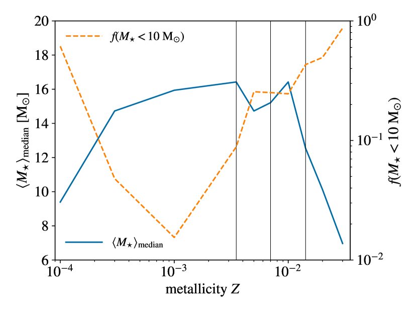
Figure 10: Median O/Be star mass (solid curve for the left axis) in Be-XRBs and fraction (dashed curve for the right axis) of Be-XRBs with low-mass ($<10\ \rm M_{\odot}$) O/Be stars in the SR_CS model. The thin vertical lines label the metallicities of the MW, LMC and SMC (from right to left).

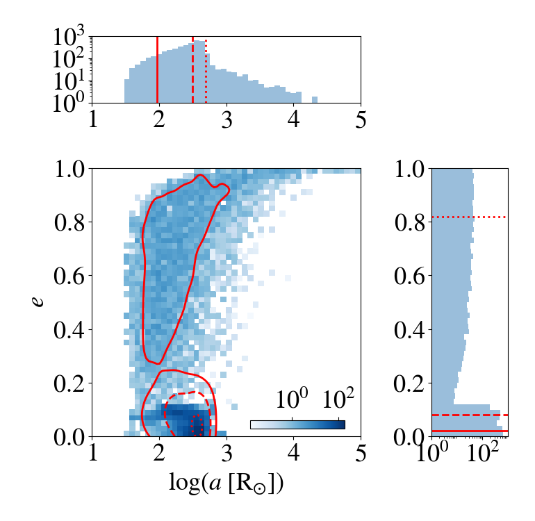
(a) $Z=10^{-4}$

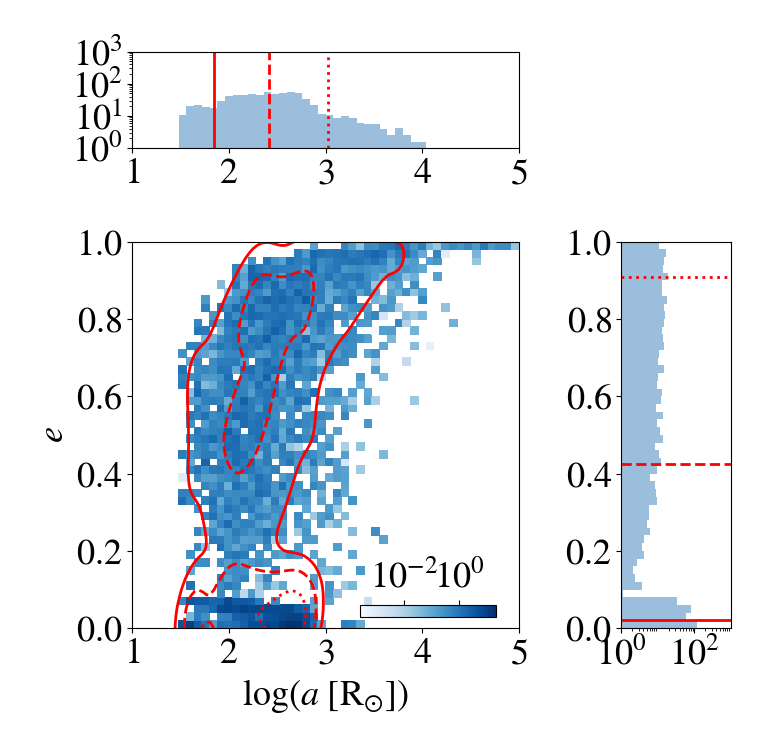
(b) $Z=0.0035$ (SMC)

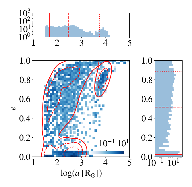
(c) $Z=0.0142$ (MW)

Figure 11: Distribution of Be-XRB orbital parameters in the SR_CS model for $Z=10^{-4}$ (left), $Z=0.0035$ (middle) and $Z=0.0142$ (right). Each Be-XRB $i$ is weighted by $\tau_{i}/M_{\rm tot}$, so that the number for each bin here corresponds to the expected number of binaries in the Be-XRB phase per unit SFR ($\rm M_{\odot}\ yr^{-1}$). In the 2D maps of joint distribution, the solid, dashed and dotted contours enclose 90%, 50% and 10% of systems from a Gaussian smoothed density field produced by the weighted data. In the marginalized distributions, the solid, dashed and dotted lines mark the 10, 50 and 90 percentiles.

We notice in Fig. 9 that there are two groups of Be-XRBs in the $\log M_{\rm X}-\log M_{1}$ space with lower and higher $M_{\rm X}$ (approximately divided by the dash-dotted lines in the bottom panels of Fig. 9) that are more distinct at higher $Z$. These two groups are also related to the complex features of Be-XRB mass distributions in the $\log M_{\rm X}-\log M_{\star}$ space. The lower-$M_{\rm X}$ group is made of binaries with relatively low-mass ($M_{1}\lesssim 25\ \rm M_{\odot}$, i.e., $\log(M_{1}\ [{\rm M_{\odot}}])\lesssim 1.4$) primary stars that always transfer significant mass to the secondary star. These binaries also cluster around a primary mass that increases with $Z$. The higher-$M_{\rm X}$ group contains both low-mass and massive primary stars. The resulting O/Be star masses cover a broader range than those from the lower-$M_{\rm X}$ group. We expect the primary stars in the lower-$M_{\rm X}$ group to completely lose their hydrogen envelope and even undergo mass transfer during the helium HG phase. In this way, most of them form low-mass NSs ($M_{\rm X}\sim 1.3\ \rm M_{\odot}$) via electron-capture SNe with no natal kicks. We find that such systems account for about half of the Be-XRBs currently in the SMC (with each simulated Be-XRB re-weighted according to the star formation history of the SMC, see Appendix A), which is consistent with the results of Vinciguerra et al. (2020). In contrast, the primary stars in the higher-$M_{\rm X}$ group keep a fraction of their hydrogen envelopes before collapse either due to higher initial masses, shorter lifetimes and/or less mass transfer in wider orbits. There is evidence of this scenario from observations of partially-stripped star + Be star binaries such as HR 6819 (Frost et al., 2022) and SMCSGS-FS 69 (Ramachandran et al., 2023). In general, both groups produce O/Be stars of a broad mass range, and the mass distribution of O/Be stars becomes bi-polar at $Z\gtrsim 0.001$, which is more obvious for O/Be stars from the higher-$M_{\rm X}$ group. This likely results from the complex dependence of the mass loss/accretion rates on primary/secondary masses and orbital parameters in BSE models, which also correlate with the natal kicks and remnant masses of primary stars, as hinted by observations (Zhao et al., 2023). We defer a through discussion on this aspect to future work.

Fig. 11 shows the orbital parameter distribution of Be-XRBs. Similarly to the results in Sec. 5.1, nearly-circular ($e\lesssim 0.1$) binaries with $a\sim 100-10^{3}\ \rm R_{\odot}$ make up a significant fraction of Be-XRBs, reaching $\sim 60\%$ at $Z=10^{-4}$. This is a natural consequence of binary interactions that tend to circularize binary orbits and our optimistic definition of the VDD boundary (Eq. 8) that allows faint objects with little accretion from beyond the tidal truncation radius to be counted as Be-XRBs (Sec. 3.1). These systems mostly belong to the aforementioned lower-$M_{\rm X}$ group and contain low-mass ($M_{\rm X}\sim 1.3\ \rm M_{\odot}$) NSs born in electron-capture SNe of helium stars with no natal kicks. Since strong mass transfer happens in their evolution histories, the O/Be stars are initially less massive and live longer than in the case of $e>0.1$. We also find that it is necessary to take into account such nearly-circular systems in order to explain the large population of Be-XRBs currently observed in the SMC, because the number of nearly-circular Be-XRBs as a function of time after a starburst has a strong peak at $\sim 30\ \rm Myr$ for $Z=Z_{\rm SMC}=0.0035$, and the SMC experienced a starburst just $\sim 20-40$ Myr ago (Rubele et al., 2015). This result is consistent with the finding in Linden et al. (2009) that Be-XRBs currently in the SMC primarily form through electron-capture SNe with low natal kicks.

If we ignore the nearly-circular binaries, our results are consistent with those in Xing & Li (2021, see their fig. 6) who define the VDD boundary with the tidal truncation radius (Eq. 7) such that nearly-circular systems are excluded. That is to say, wide ($a\gtrsim 300\ \rm R_{\odot}$) binaries with longer $a$ need to have higher $e$ to interact with the VDD at the pericenter. On the other hand, there is an upper limit of $e$ that increases with $a$ in close binaries ($a\lesssim 300\ \rm R_{\odot}$) to avoid RLO of the O/B star. Finally, we find that the distribution of $a$ is broader at higher $Z$, while the median is almost constant at $a\sim 300\ \rm R_{\odot}$. The increase of the fraction of wide Be-XRBs at higher $Z$ can be explained by the stronger winds that widen binary orbits more significantly. The increasing relative importance of very close binaries ($a\lesssim 100\ \rm R_{\odot}$) at higher $Z$ corresponds to the decreasing importance of the lower-$M_{\rm X}$ group that produces a stronger peak around $a\sim 500\ \rm R_{\odot}$ at lower $Z$, and the trend will disappear if we exclude nearly-circular binaries.

5.3 X-ray outputs

Table 3: X-ray luminosity per unit SFR as a function of metallicity $Z$ for the 4 models defined in Table 2 with $f_{\rm corr}=0.5$, in terms of $\log(\mathcal{L}_{\rm X}\equiv\langle L_{\rm X}\rangle/{\rm SFR}\ [\rm\ erg\ s^{-1}\ M_{\odot}^{-1}\ yr])$, in 4 energy bands: $0.1-2$ keV, $0.5-2$ keV, $2-10$ keV and $0.5-8$ keV, as well as for the bolometric luminosity.

Absolute metallicity $Z$	0.0001	0.0003	0.001	0.0035	0.005	0.007	0.01	0.0142	0.02	0.03
SR_CS
$0.1-2$ keV	39.73	39.57	39.48	39.35	39.22	39.09	39.00	38.78	38.63	37.67
$0.5-2$ keV	39.70	39.54	39.45	39.33	39.20	39.07	38.98	38.75	38.60	37.64
$2-10$ keV	40.07	39.90	39.81	39.70	39.59	39.47	39.37	39.16	39.01	38.07
$0.5-8$ keV	40.19	40.02	39.93	39.82	39.70	39.58	39.48	39.27	39.12	38.17
Bolometric	40.43	40.26	40.17	40.06	39.96	39.84	39.74	39.53	39.38	38.44
FR_CS
$0.1-2$ keV	39.78	39.62	39.55	39.40	39.36	39.23	39.05	38.96	38.61	37.65
$0.5-2$ keV	39.75	39.59	39.51	39.37	39.33	39.21	39.02	38.94	38.58	37.62
$2-10$ keV	40.12	39.94	39.87	39.74	39.70	39.59	39.41	39.32	39.00	38.10
$0.5-8$ keV	40.24	40.07	40.00	39.86	39.82	39.71	39.53	39.44	39.10	38.18
Bolometric	40.48	40.30	40.23	40.11	40.07	39.96	39.79	39.69	39.37	38.48
SR_OP
$0.1-2$ keV	40.33	40.17	40.05	39.94	39.77	39.52	39.17	38.78	38.63	37.67
$0.5-2$ keV	40.30	40.14	40.02	39.91	39.75	39.49	39.15	38.75	38.60	37.64
$2-10$ keV	40.63	40.44	40.33	40.22	40.08	39.85	39.52	39.16	39.01	38.07
$0.5-8$ keV	40.77	40.59	40.47	40.37	40.22	39.98	39.64	39.27	39.12	38.17
Bolometric	40.98	40.79	40.68	40.58	40.44	40.22	39.89	39.53	39.38	38.44
FR_OP
$0.1-2$ keV	40.40	40.26	40.17	40.05	39.88	39.64	39.29	38.96	38.61	37.65
$0.5-2$ keV	40.37	40.23	40.14	40.02	39.86	39.62	39.26	38.94	38.58	37.62
$2-10$ keV	40.68	40.53	40.44	40.32	40.17	39.95	39.63	39.32	39.00	38.10
$0.5-8$ keV	40.83	40.68	40.59	40.47	40.31	40.09	39.75	39.44	39.10	38.18
Bolometric	41.04	40.87	40.78	40.67	40.52	40.31	39.99	39.69	39.37	38.48

To characterize the X-ray outputs from the simulated Be-XRB populations, we start with the time evolution of total X-ray luminosity per unit stellar mass from an instantaneous starburst (at $t=0$):

$$\frac{\bar{L}^{\rm tot}_{\nu}(t)}{M_{\rm tot}}=\frac{\sum_{i}^{N}f_{{\rm duty},i}L_{\nu,i}\Theta(t-t_{i,\rm ini})\Theta(t_{i,\rm fin}-t)}{M_{\rm tot}}\ ,$$ (23)

where Be-XRB $i$ lives from $t_{i,\rm ini}$ to $t_{i,\rm fin}$ with a (specific) luminosity $L_{\nu,i}$ during outbursts for a certain energy (band) and a duty cycle $f_{{\rm duty},i}$, and $\Theta$ is the Heaviside step function. Fig. 12 shows the results for the $0.5-8$ keV band from the SR_CS model with $f_{\rm corr}=0.5$ at 4 representative metallicities. There is a delay of $\sim 3-10$ Myr between the starburst and the onset of X-ray emission from Be-XRBs, which reflects the evolutionary time for (the most) massive primary stars in Be-XRB progenitors to become compact objects. The total X-ray luminosity peaks at a few Myr after the starburst for $Z\lesssim 0.01$, while the peak (as well as the onset) of X-ray emission shifts to later stages at higher $Z$, up to $\sim 20$ Myr for $Z=0.03$. This is caused by the suppression of Be-XRBs from massive binaries by stellar winds that is more significant at higher $Z$ (see Sec. 5.2) and longer lifetimes of (initially less massive) primary stars in Be-XRB progenitors with higher $Z$. The X-ray luminosity drops by at least 2 orders of magnitude within 100 Myr post the peak. The most metal-poor model with $Z=10^{-4}$ has a much slower drop compared with the other cases due to a higher fraction of Be-XRBs with low-mass Be stars from low-mass progenitors (see Figs. 9 and 10).

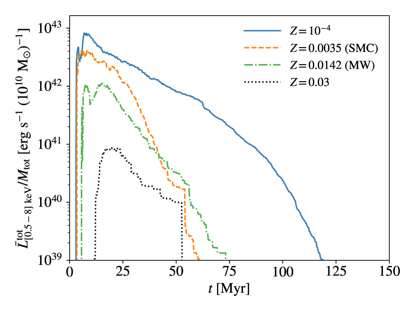
Figure 12: Evolution of X-ray luminosity in the $0.5-8$ keV band per unit stellar mass from Be-XRBs formed by an instantaneous starburst in the SR_CS model with $f_{\rm corr}=0.5$, for $Z=10^{-4}$ (solid), 0.0035 (dashed), 0.0142 (dash-dotted) and 0.03 (dotted). Here $t=0$ corresponds to the moment of starburst.

Now, given the short-lived nature of Be-XRBs, their overall X-ray output can be well characterized by the (specific) X-ray luminosity per unit SFR:

$$\mathcal{L}_{\nu} \equiv\frac{\langle L_{\nu}\rangle}{{\rm SFR}}=\sum_{i}^{N}\left(\frac{f_{{\rm duty},i}\tau_{i}}{M_{\rm tot}}\right)L_{\nu,i}\ ,$$ (24)

where $\tau_{i}=t_{i,\rm fin}-t_{i,\rm ini}$ is the duration of the Be-XRB phase for binary $i$. Fig. 13 shows the full (intrinsic) SEDs in terms of $\nu\mathcal{L}_{\nu}$ for $Z=10^{-4}$ and 0.0142, in the SR_CS model with $f_{\rm corr}=0.5$, where we also plot the contributions of different types of outbursts (Type I and II, see Sec. 3.2), accretion regimes (LH, HS and SE, see Sec. 4) and compact objects (NS and BH). In general, for the photon energy range $E\sim 0.5-8$ keV that typically contains $\sim 60\%$ of the integrated bolometric luminosity from a Be-XRB population, the SED is always dominated by NSs in the SE regime with $\eta>2$ mostly via Type II outbursts, and the contribution of BHs remains below 10%. This means that the spectral shape is almost independent of $Z$ in this energy range and the majority of X-ray emission comes from luminous ($\gtrsim 10^{38}\ \rm erg\ s^{-1}$) systems. In fact, SE systems contribute $\sim 55-68$% of the total bolometric luminosity per unit SFR for $Z\in[10^{-4},0.03]$ with mildly increasing importance at lower $Z$. Similarly, Type II outbursts make up $\sim 56-71$% of the total X-ray output due to their luminous nature, even though the number fraction of all (active) Type II systems is (much) lower, $\sim 13-44\ (2-16$)%. For more energetic photons ($E\gtrsim 8$ keV), the contribution from NSs in the HS regime ($\eta\sim 0.05-2$) becomes important due to their harder spectra, especially at higher $Z$, while for $E\lesssim 0.1$ keV, BHs (mostly in the SE regime during Type II outbursts) dominate the spectrum when they exist in Be-XRBs at $Z\lesssim 0.001$.

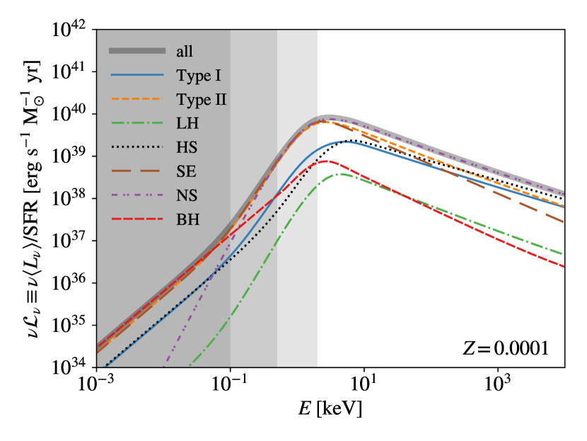
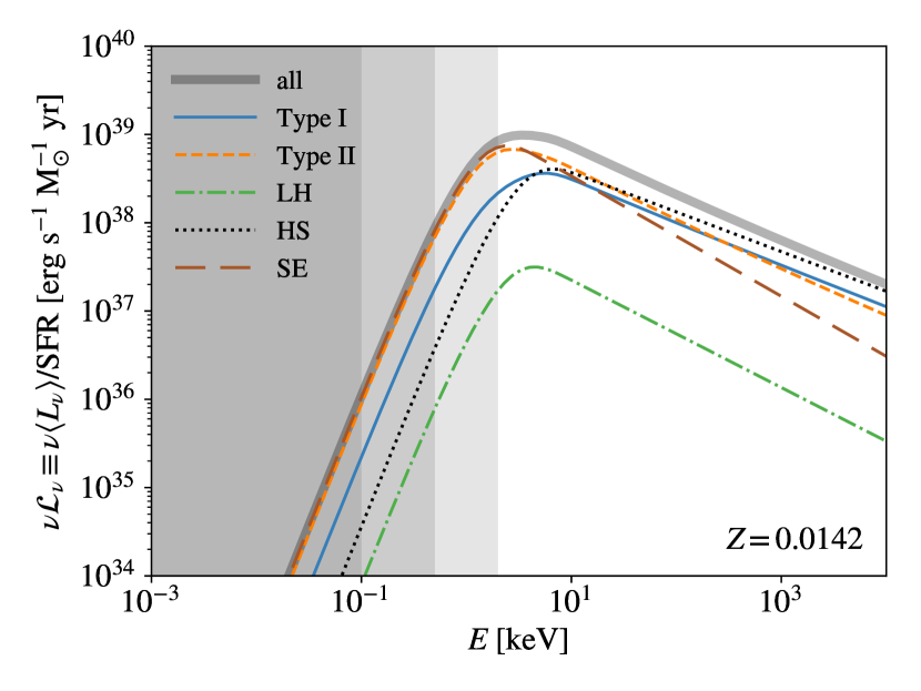
Figure 13: SED of Be-XRBs per unit SFR from the SR_CS model with $f_{\rm corr}=0.5$ at $Z=10^{-4}$ (top) and 0.0142 (bottom). The total spectrum is shown with the thick solid curve. Contributions from Type I and II outbursts are denoted by the solid and dashed curves. Components of the LH, HS and SE states are shown with the dash-dotted, dotted and long-dashed curves. In the $Z=10^{-4}$ case where BHs are present, we show the NS and BH contributions with the dash-dot-dotted and densely-dashed curves. The shaded regions show different levels of absorption as defined in Fig. 6.

Next, to better evaluate the metallicity dependence, we calculate the X-ray luminosity per unit SFR in select energy bands for each simulated Be-XRB population. We start with two energy bands with very-soft ($0.1-2$ keV) and soft ($0.5-2$ keV) X-rays that are expected to escape the host haloes and interact with the IGM at $z\gtrsim 20$ and $z\sim 10$, respectively (Das et al., 2017; Sartorio et al., 2023). We further consider a hard band ($2-10$ keV) and a broad band ($0.5-8$ keV) to make comparison with literature results (see below). Fig. 14 shows the X-ray luminosity per unit SFR as a function of $Z$ in these 4 bands for the SR_CS model with $f_{\rm corr}=0.5$. The results for all the 4 models in Table 2 are summarized in Table 3.

5.3.1 Be-XRBs VS other types of HMXBs

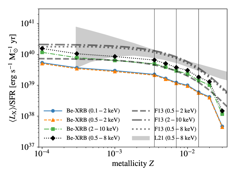
Figure 14: X-ray luminosity per unit SFR of Be-XRBs in the SR_CS model with $f_{\rm corr}=0.5$, in the energy bands $E\sim 0.1-2$ (solid), $0.5-2$ (dashed), $2-10$ (dash-dotted) and $0.5-8$ keV (dotted). For comparison, we plot the best-fit models from BPS results for other types of HMXBs in Fragos et al. (2013b, F13) with the thick curves following the same line styles for the latter three bands. Here for the $0.5-2$ keV and $2-10$ keV bands, we use the fitting formulae and parameters in their eq. 3 and table 2, while the results for the $0.5-8$ keV band are taken from Lehmer et al. (2021, see their fig. 4). The observational results for the $0.5-8$ keV band from Lehmer et al. (2021, L21, see their fig. 4 and table 3) are shown with the shaded region. The thin vertical lines label the metallicities of the MW, LMC and SMC (from right to left).

We first compare our predictions for Be-XRBs with the BPS results for other types of HMXBs powered by RLO and (spherical) stellar winds (Fragos et al., 2013b). As shown in Fig. 14, we find that (at the same $Z$) the X-ray luminosity (per unit SFR) from Be-XRBs in our SR_CS model with $f_{\rm corr}=0.5$ is comparable (lower by up to a factor of 3) to that from other types of HMXBs predicted by Fragos et al. (2013b) for $Z\sim 0.001-0.02$, where the evolution with $Z$ is also similar. This indicates that Be-XRBs can be as important as other types of HMXBs. Moreover, the striking similarity between the metallicity dependence of X-ray outputs in the two populations of HMXBs powered by distinct mechanisms (decretion disks of O/Be stars VS RLO and stellar winds) can be understood by the fact that their key properties (number counts and accretion rates of compact objects) are determined by the same binary stellar evolution processes (e.g., stellar winds, mass transfer and SN natal kicks) in this metallicity range.

However, at $Z\lesssim 0.001$ and $Z\gtrsim 0.02$, our results for Be-XRBs show stronger evolution with $Z$. In Fragos et al. (2013b), the X-ray luminosity from other types of HMXBs is almost constant for $Z\lesssim 0.001$, while in our case, the X-ray luminosity from Be-XRBs increases by a factor of $\sim 2$ from $Z=0.001$ to $Z=10^{-4}$. The rapid drop of X-ray luminosity at $Z>0.02$ in our case is caused by the stronger stellar winds at higher $Z$ that significantly reduce the number of (luminous) Be-XRBs (see Figs. 7 and 8), such that the predicted X-ray output has large errors ($\sim 0.5$ dex) due to the poor statistics of luminous Be-XRBs. In fact, the X-ray output of the $Z=0.03$ model can be enhanced by a factor of $\sim 10$ when using the wind model in Hurley et al. (2002) that predicts weaker winds at high $Z$ than considered in our default wind prescription based on Schneider et al. (2018) and Sander & Vink (2020). However, the effect of varying wind models on the total X-ray output is much weaker at lower metallicities (within factors of $\sim 3$ and $\sim 20$% for $Z\lesssim 0.02$ and $Z\lesssim 0.005$, respectively).

The difference between our results and those in Fragos et al. (2013b) only varies slightly with the energy band considered, with the broad band ($0.5-8$ keV) having the smallest difference and the hard band ($2-10$ keV) the largest. This indicates that the overall SEDs of Be-XRB populations in our case are similar to those in Fragos et al. (2013b) for other types of HMXBs. For instance, we have $L_{\rm[0.5-2]\ keV}/L_{\rm[2-10]\ keV}\simeq 0.41$, and this ratio is $\simeq 0.35$ in Fragos et al. (2013b). The small difference is caused by the different X-ray spectral models adopted in our work (Fig. 13) and by Fragos et al. (2013b, see their fig. 1). The latter predict slightly harder spectra with stronger X-ray emission at $E\gtrsim 2$ keV. The reason is that their spectral model (Fragos et al., 2013a) only considers the LH and HS regimes and is calibrated to the BC factors derived from the early samples of Galactic XRBs in McClintock & Remillard (2006) and Wu et al. (2010), while our model further includes the SE regime (which is dominant for Be-XRBs) and adopts the recent observational data for BC factors in Anastasopoulou et al. (2022).

5.3.2 Comparison with HMXBs observed in nearby galaxies

Next, we compare the overall X-ray outputs from our Be-XRB populations with observational results for HMXB populations in nearby galaxies (Douna et al., 2015; Lehmer et al., 2021). Assuming that observations are complete, we find that the simulated Be-XRBs in our fiducial model (SR_CS with $f_{\rm corr}=0.5$) can explain $\sim 60\%$ of the observed X-ray luminosity of (all types of) HMXBs in nearby galaxies (Lehmer et al., 2021), with a similar metallicity dependence (see the shaded region in Fig. 14). The X-ray luminosity increases by about one order of magnitude from $Z\sim 0.02$ to $Z\lesssim 0.0003$. This is consistent with the results in Sec. 5.1 for number counts of ultra-luminous HMXBs with $L_{[0.5-8]~{}\rm keV}>10^{39}\ \rm erg\ s^{-1}$ (Fig. 8). It is shown in Appendix B that both the observed number of (ultra-)luminous HMXBs and overall X-ray luminosity per unit SFR from Lehmer et al. (2021, for all types of HMXBs) can be fully reproduced by our SR_CS model of Be-XRBs at $Z\sim 0.0003-0.02$, if given a higher correction factor $f_{\rm corr}=0.8$ than that assumed by default ($f_{\rm corr}=0.5$). This is non-trivial because systems with $L_{[0.5-8]~{}\rm keV}>10^{39}\ \rm erg\ s^{-1}$ only account for $\sim 15-50$% of the total X-ray output in our Be-XRB populations at $Z\sim 0.0003-0.02$ from the SR_CS model with $f_{\rm corr}\sim 0.25-0.8$. Moreover, this indicates that $f_{\rm corr}\gtrsim 0.8$ is ruled out in our SR_CS model, considering that other types of HMXBs also contribute to the observed values.

Finally, we calculate the X-ray luminosity per luminous Be-XRB with $L_{[0.5-8]~{}\rm keV}>10^{38}\ \rm erg\ s^{-1}$ in the $0.5-8$ keV band $\langle L_{\rm[0.5-8]\ keV}^{38}\rangle/\langle N_{\rm X}^{38}\rangle$, as shown in Fig. 15 for all the 4 models in Table 2 assuming $f_{\rm corr}=0.5$. In general, we have $\langle L_{\rm[0.5-8]\ keV}^{38}\rangle/\langle N_{\rm X}^{38}\rangle\sim 0.5-1\times 10^{39}\ \rm erg\ s^{-1}$, insensitive to both metallicity and model parameters even with variations of $f_{\rm corr}$ in the range of $[0.25,1]$ (not shown for conciseness). Our results are consistent with observations of HMXBs in nearby galaxies for $Z\sim 0.0004-0.03$ (Douna et al., 2015, see their fig. 5), which further implies that the luminous X-ray sources in our Be-XRB populations are similar to those in observed HMXB populations.

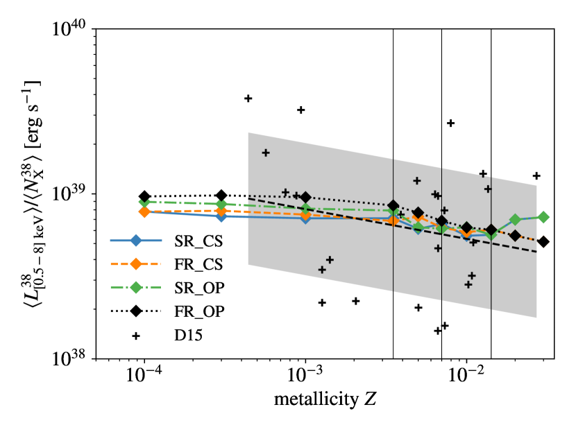
Figure 15: X-ray luminosity per luminous Be-XRBs with $L_{[0.5-8]~{}\rm keV}>10^{38}\ \rm erg\ s^{-1}$, for the SR_CS (solid), FR_CS (dashed), SR_OP (dash-dotted) and FR_OP (dotted) models with $f_{\rm corr}=0.5$. The observational data from nearby galaxies and the corresponding power-law fit from Douna et al. (2015, D15, see their fig. 5) are shown with the crosses and dashed line surrounded by the shaded region. The thin vertical lines label the metallicities of the MW, LMC and SMC (from right to left).

6 Caveats

To quantify more accurately the roles played by Be-XRBs, particularly in the ULX population (e.g., Kaaret et al., 2017; Kovlakas et al., 2020; Fabrika et al., 2021; Walton et al., 2022; King et al., 2023; Salvaggio et al., 2023; Tranin et al., 2023; Misra et al., 2023a), and their imprints in the early Universe, more work needs to be done to overcome the following caveats of our study (with descending order of importance).

1. Although being more complete compared with previous studies, our model of the X-ray outbursts in Be-XRBs still relies on a phenomenological model based on simulations of steady-state VDDs with constant mass ejection rates (Eq. 19) and viscosity. However, in reality VDDs of O/Be stars, especially under the influence of companions, can be highly dynamical structures (Carciofi & Bjorkman, 2008; Haubois et al., 2012; Krtička et al., 2015; Panoglou et al., 2016; Vieira et al., 2017; Rímulo et al., 2018), with variable mass ejection and disk dissipation/formation episodes of a few years (Reig, 2011). Such dynamical evolution of disk structures are particularly important for the most luminous Be-XRBs with non-periodic, strong Type II outbursts (see Sec. 3.2.2). In fact, according to our steady-state model, the majority ($\sim 60-70\%$) of X-ray emission from Be-XRBs are produced by the systems in which the compact object is able to accrete almost all ($\gtrsim 90$%) of the materials ejected from the O/B star, so that significant variations of disk structures are expected to occur. Additional uncertainties of our model may reside in the interpretation of simulation results and comparison with observations, as we do not model the detailed structure of accretion flows and geometry of X-ray emission, which are complex and still in debate, especially for ULXs (Wiktorowicz et al., 2019; Fabrika et al., 2021; Mushtukov & Tsygankov, 2022; King et al., 2023; Lasota & King, 2023). For instance, taking into account the suppression of accretion by radiation-driven winds in the super-Eddington regime (Shakura & Sunyaev, 1973) reduces the X-ray outputs and number counts of ULXs from our Be-XRB populations by up to $\sim 60$% and a factor of $\sim 10$, respectively.

2. We do not fully explore the parameter space of (binary) stellar evolution. Although the mass-transfer efficiency in our BPS runs is calibrated to reproduce the number and range of orbital periods of Be-XRBs observed in the SMC, the agreement with observations is imperfect, and the other parameters (fixed in our case) governing the mass loss rate from stellar winds, stability of mass transfer, angular momentum loss, spin-up of the accretor, as well as natal kicks of SNe may affect Be-XRB properties and final X-ray outputs greatly (see, e.g., Linden et al., 2009; Zuo et al., 2014; Shao & Li, 2014, 2020; Vinciguerra et al., 2020; Xing & Li, 2021; Misra et al., 2023b; Willcox et al., 2023). For instance, recent parallax and proper-motion measurements of young, isolated radio pulsars and Galactic Be-XRBs have placed new constraints on SN natal kicks. These support a kick-velocity distribution that is the sum of two Maxwellian distributions with $\sigma_{\rm kick}\sim 50$ and $340\ \rm km\ s^{-1}$, where the low-$\sigma_{\rm kick}$ component accounts for $20\pm 10$% of all systems (Verbunt et al., 2017; Igoshev et al., 2021). Our model of natal kicks is qualitatively consistent with these results given the separate treatments of electron-capture SNe (with $\sigma_{\rm kick}=0$) and high-$\sigma_{\rm kick}$ cases (Type II and Ib/c with $\sigma_{\rm kick}=190$), although our $\sigma_{\rm kick}$ are smaller. We find by numerical experiments that compared with our default case, using the best-fit model of kick-velocity distribution in Igoshev et al. (2021) with generally stronger kicks will reduce the X-ray output from Be-XRBs by up to a factor of $\sim 3$ for $Z\lesssim 0.02$. However, with the kick-velocity distribution from Igoshev et al. (2021), Be-XRBs on nearly circular ($e\lesssim 0.1$) orbits become extremely rare ($\lesssim 4$%), and the predicted number of Be-XRBs in the SMC is lower by a factor of $\sim 2$ than that observed (see Appendix A). We defer a more detailed investigation into the effects of SN natal kicks on the X-ray output from Be-XRBs to future work. The prescription of stellar winds is also important, especially for metal-rich stellar populations, causing up to one order of magnitude variations in the X-ray output at $Z=0.03$ (see Sec. 5.3.1).

3. In the construction of our binary populations, we do not consider the correlations between initial binary properties (i.e., binary fraction, distributions of masses and orbital parameters) nor their metallicity dependence, while there is evidence/hints of such correlations and evolution with metallicity from observations and simulations (e.g., Gunawardhana et al., 2011; Marks et al., 2012; Duchêne & Kraus, 2013; Moe & Di Stefano, 2017; Moe et al., 2019; Jeřábková et al., 2018; Lacchin et al., 2020; Chon et al., 2021; Chon et al., 2022; Tanvir & Krumholz, 2023; Rusakov et al., 2023). Taking these effects into account may modify the predicted evolution of X-ray luminosity with metallicity and change our finding that the total X-ray output from Be-XRBs is insensitive to initial conditions.

4. The effects of rotation on stellar evolution are not considered in our BPS runs, although it is shown by detailed stellar-evolution simulations (e.g., Ekström et al., 2012; Georgy et al., 2013; Choi et al., 2017; Groh et al., 2019; Murphy et al., 2021) that fast rotation can impact the mass loss, timescales of evolution phases, stellar structure, nucleosynthesis and remnant masses in a complex and metallicity-dependent manner, particularly for initially fast-rotating stars, which can also change the properties of Be-XRBs that by definition contain fast-rotating O/B stars.

5. We use simple models calibrated to observations to derive the X-ray spectra of Be-XRBs, which only consider three regimes of accretion rates (low-hard, high-soft and super-Eddington) for two types of compact objects (NSs and BHs), while in reality, the X-ray spectra of Be-XRBs can have more complex dependence on compact object properties (e.g., masses, spins and magnetic fields) and accretion modes (e.g., thin disk and ADAF) that may also correlate with the stellar and orbital parameters as well as types of outbursts (Martin et al., 2011; Okazaki et al., 2013; Cheng et al., 2014; Haberl & Sturm, 2016; Xu & Li, 2019; Franchini & Martin, 2021).

7 Summary and conclusions

We improve population synthesis of Be-XRBs with a physically motivated model that combines recent hydrodynamic simulations of VDDs in Be-XRBs (Brown et al., 2019) and VDD properties inferred from observations of classical Be stars (Vieira et al., 2017; Rímulo et al., 2018). Our model for the first time fully takes into account the dependence of X-ray outburst properties (i.e., strength and duty cycle) on stellar and orbital parameters of Be-XRBs, and also considers the classification of X-ray outbursts into the two conventional types in observations (Reig, 2011; Rivinius et al., 2013). Using the standard BSE models (Hurley et al., 2002) in the BPS code binary_c, we evolve large populations of randomly sampled massive binaries in the (absolute) metallicity range $Z\in[10^{-4},0.03]$ with initial conditions and BSE parameters calibrated to reproduce the population of observed Be-XRBs in the SMC (see Appendix A). Finally, we apply an X-ray spectral model based on recent observations of HMXBs (Anastasopoulou et al., 2022) to our simulated Be-XRBs to evaluate the X-ray luminosity per unit SFR from Be-XRBs as a function of metallicity. The effects of free model parameters for initial conditions and VDD densities are also explored. Our main findings are summarized as follows.

1. Be-XRBs can probably explain a non-negligible fraction of the total X-ray output from HMXBs observed in nearby galaxies (Lehmer et al., 2021). Assuming that current observations are complete, the X-ray luminosities per unit SFR from our simulated Be-XRB populations are at least $\sim 30\%$ of the observed values for all types of HMXBs at $Z\sim 0.0003-0.02$. The minimum fraction $\sim 30\%$ is reached with the minimum correction factor $f_{\rm corr}=0.25$ allowed in our Be-XRB model calibrated to the observed relation between outburst X-ray luminosity and orbital period (Sec. 3.2.1), and is subject to uncertainties from our imperfect modelling of VDDs, the limited parameter space of BPS explored, and the fact that our BPS simulations only consider Be-XRBs rather than all types of HMXBs (see Sec. 6). In our fiducial model with no $Z$ dependence of VDD densities nor enhanced initial stellar rotation, the X-ray luminosity per unit SFR decreases by a factor of $\sim 8$ from $Z=0.0003$ to $Z=0.02$, which is mainly driven by the stronger stellar winds at higher $Z$ that reduce the number of binary stars able to become luminous Be-XRBs. Interestingly, this trend is similar to that seen in observations of all types of HMXBs.

2. Our results for Be-XRBs are also similar to the $Z$-dependent X-ray outputs from other types of HMXBs powered by RLO and (spherical) stellar winds in previous BPS studies (e.g., Fragos et al., 2013b) for $Z\sim 0.001-0.02$ (Sec. 5.3.1). However, at $Z\lesssim 0.001$, the X-ray luminosity from Be-XRBs keeps increasing towards lower $Z$ (e.g., by a factor of $\sim 2$ from $Z=0.001$ to $Z=10^{-4}$), while there is almost no evolution in that from other types of HMXBs predicted by Fragos et al. (2013b). This implies that Be-XRBs might play more important roles at lower metallicities, such that they can have strong impact on the thermal history and thus 21-cm signal from the IGM at Cosmic Dawn. More comprehensive BPS studies that consider both Be-XRBs and other types of HMXBs self-consistently are required to verify if this is indeed the case.

3. Luminous ($\gtrsim 10^{38}\ \rm erg\ s^{-1}$) systems with non-periodic, major outbursts of Type II (see Sec. 3.2.2 for a detailed definition) and super-Eddington accretion (mostly on eccentric orbits with $e\gtrsim 0.4$), including ULXs ($\gtrsim 10^{39}\ \rm erg\ s^{-1}$), are important X-ray powerhouses in our Be-XRB populations across the metallicity range considered. In our fiducial model, $\sim 55-75\%$ of the total X-ray output of Be-XRBs comes from luminous sources with $L_{[0.5-8]\ \rm keV}>10^{38}\ \rm erg\ s^{-1}$, while ULXs with $L_{[0.5-8]\ \rm keV}>10^{39}\ \rm erg\ s^{-1}$ contribute $\sim 24-41\%$ of the total output. Similarly to the case of total X-ray output, the simulated Be-XRBs can also account for non-negligible fractions of the number counts of luminous and ultra-luminous HMXBs in observations (Mapelli et al., 2010; Douna et al., 2015; Kovlakas et al., 2020; Lehmer et al., 2021), although more work needs to be done to fully evaluate the contributions of Be-XRBs. Such luminous systems have been overlooked in previous BPS studies of Be-XRBs (e.g., Zuo et al., 2014; Misra et al., 2023b), which use a simple empirical scaling law between outburst X-ray luminosity and orbital period (Dai et al., 2006, see our Eq. 12 and Fig. 3) that imposes a (likely artificial) cutoff at $\sim 10^{38}\ \rm erg\ s^{-1}$, while our improved Be-XRB model further considers the dependence of outburst accretion rate/luminosity on VDD density (and its scatter) as well as orbital eccentricity, so that the luminosity function of our Be-XRBs has a luminous tail up to $10^{41}\ \rm erg\ s^{-1}$, as shown in Fig. 16.

4. The major uncertainty in the total X-ray output from Be-XRBs arises from the uncertainties in accretion rates and VDD properties rather than those in initial conditions when fixing the IMF (see Sec. 2.3). The former can change the final X-ray output by a factor of a few, while the difference made by the latter is within $\sim 50$% (see Sec. 5.1 and Appendix B). The reason is that the X-ray luminosity of an accreting compact object is proportional to the accretion rate, which is then proportional to the VDD density (or mass ejection rate of the O/B star) to the first order, and there are still large uncertainties in these quantities from idealized simulations and limited observations, especially at low metallicity. On the other hand, a key feature of our BPS simulations is that in most binaries that can potentially become Be-XRBs the secondary star will be spun up to become an O/Be star (via stable mass transfer) regardless of its initial rotation rate, which is consistent with the scenario that most (young) O/Be stars are produced by binary interactions as predicted/hinted by theoretical models and observations (Shao & Li, 2014; Klement et al., 2019; Bodensteiner et al., 2020; Dorigo Jones et al., 2020; Hastings et al., 2020; Hastings et al., 2021; Dallas et al., 2022; Dodd et al., 2023; Wang et al., 2023).

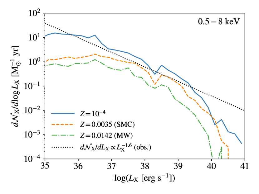
Figure 16: X-ray luminosity function (per unit SFR) of Be-XRBs in the 0.5-8 keV band predicted by our fiducial model (SR_CS with $f_{\rm corr}=0.5$) for $Z=10^{-4}$ (solid), 0.0035 (dashed) and 0.0142 (dash-dotted). Here each Be-XRB is weighted by $f_{{\rm duty},i}\tau_{i}/M_{\rm tot}$. The power-law fit ($d\mathcal{N}_{\rm X}/dL_{\rm X}\propto L_{\rm X}^{-1.6}$) to the average X-ray luminosity function of observed HMXBs in star-forming galaxies (Mineo et al., 2012, see their fig. 5) is plotted with the dotted line for comparison. The X-ray luminosity functions of our Be-XRBs are generally consistent with the observed power-law shape for $L_{\rm X}\sim 10^{36}-10^{39}\ \rm erg\ ^{-1}$, while the number fractions of systems in both the faint and luminous ends are lower for our Be-XRBs compared with the whole population of HMXBs in observations.

In general, our BPS results highlight the possibility that Be-XRBs constitute an important component in the population of HMXBs, making significant contributions to the overall X-ray output and number count of ULXs.

Indeed, robust modelling of XRBs with BPS is a challenging task (see Sec. 6) because of large uncertainties in binary stellar evolution, particularly for Be-XRBs due to their transient nature and our lack of understanding on the detailed mechanisms that drive the formation and evolution of VDDs around fast-rotating massive stars (for candidate scenarios, see, e.g., Granada et al., 2013; Hastings et al., 2020; Zhao & Fuller, 2020; Cranmer, 2009; Rogers et al., 2013; Lee et al., 2014; Ressler, 2021). Nevertheless, such theoretical efforts are worthwhile considering the important roles played by XRBs in the Epoch of Reionization and Cosmic Dawn (e.g., Fialkov et al., 2014; Fialkov & Barkana, 2014; Pacucci et al., 2014), as well as the wealth of high-$z$ observational data to come in the next decades for the 21-cm signal by radio telescopes such as HERA (DeBoer et al., 2017), SARAS (Singh et al., 2022), REACH (de Lera Acedo et al., 2022), NenuFAR (Mertens et al., 2021), MIST (Monsalve et al., 2023) and SKA (Koopmans et al., 2015) which will place constraints on high-$z$ XRBs and the underlying star/galaxy/structure formation processes.

The present paper is a small step that points out the importance of Be-XRBs. In future work, we plan to model Be-XRBs (with possible improvements of the aforementioned caveats) and other types of XRBs in one BPS framework to predict their impact on the 21-cm signal as well as cosmic X-ray background and derive constraints from existing observational data (e.g., Lehmer et al., 2012; Moretti et al., 2012; Cappelluti et al., 2017; Fialkov et al., 2017; Bowman et al., 2018; Bevins et al., 2023; Lazare et al., 2023; Rossland et al., 2023). We will also extend the metallicity range down to the extremely metal-poor ($Z\lesssim 10^{-6}$) regime of Pop III stars, which are expected to be promising progenitors of Be-XRBs (Sartorio et al., 2023) given their compact and fast-rotating nature that favors stable mass transfer (Inayoshi et al., 2017) and formation of O/Be stars. Another interesting topic to investigate is the connection between (Be-)XRBs and compact object mergers (see, e.g., Marchant et al., 2017; Mondal et al., 2020; Fishbach & Kalogera, 2022; Kotko & Belczynski, 2023; Liotine et al., 2023) that may foster the synergy between 21-cm and gravitational wave observations to better constrain binary stellar evolution in high-$z$ galaxies.

Data availability

The data of Be-XRBs and python scripts used to manage BPS runs and conduct post-processing will be shared on reasonable request to the corresponding authors. The BPS code binary_c (including the Be-XRB module) is available at https://gitlab.com/binary_c/binary_c/-/tree/development-BeXRB. The corresponding python interface binary_c-python is available at https://gitlab.com/binary_c/binary_c-python/-/tree/feature/source_file_sampling.

Appendix A Be-XRBs in the SMC

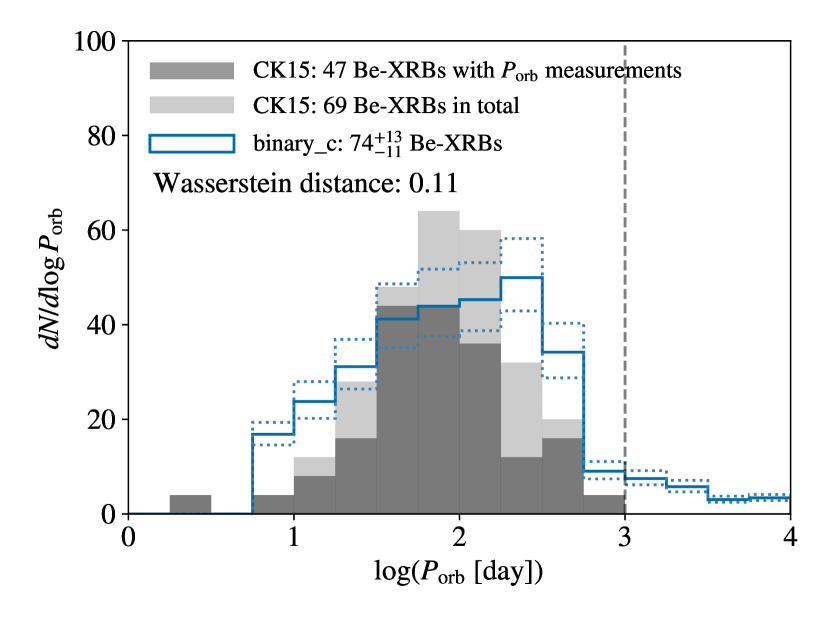
Figure 17: Orbital period distribution of Be-XRBs in the SMC predicted by the SR_CS model (contours) with the default initial binary statistics, compared with the observed population (histograms) from Coe & Kirk (2015, CK15). The solid contour shows the most likely case, enclosed by the dotted contours that reflect the uncertainties of the SMC star formation history (Rubele et al., 2015). The darker histograms show the distribution for the 47 Be-XRBs with measurements of $P_{\rm orb}$, while the lighter histograms also include the 22 Be-XRBs with $P_{\rm orb}$ inferred from the empirical scaling law $\log(P_{\rm orb}\ [{\rm day}])=0.4329\log(P_{\rm s}\ [{\rm s}])+1.043$ (Vinciguerra et al., 2020) given the spin period $P_{\rm s}$. The SR_CS model predicts $74_{-11}^{+13}$ Be-XRBs with $P_{\rm orb}<10^{3}$ days (dashed vertical line) in the SMC, consistent with the number 69 in observations. The predicted and observed distributions at $P_{\rm orb}<10^{3}$ days agree well with a Wasserstein distance of 0.11.

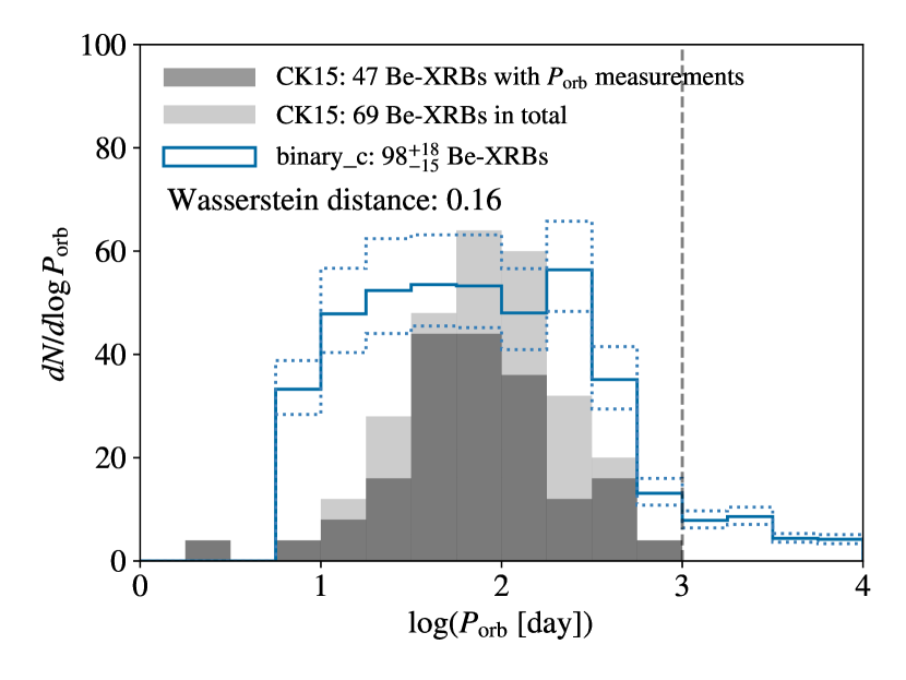
Figure 18: Same as Fig. 17 but for the FR_CS model with enhanced initial rotation (see Table 2). The FR_CS model predicts more Be-XRBs, $N_{\rm BeXRB}=98_{-15}^{+18}$, compared with the SR_CS model. However, the over-predication of low-period systems in the FR_CS model is more significant, leading to a larger Wasserstein distance of 0.16.

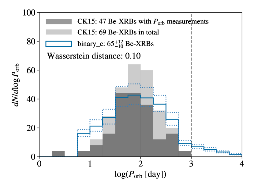
Figure 19: Same as Fig. 17 but for the SR_CS model with the hybrid initial orbital period distribution (Eqs. 2-4). Now we have $N_{\rm BeXRB}=65_{-10}^{+12}$, lower than the number $74_{-11}^{+13}$ in the default case, but still consistent with observations. The observed $P_{\rm orb}$ distribution is better reproduced with a slightly smaller Wasserstein distance of 0.1 than in the default case.

As mentioned in Sec. 2, the BSE parameters and initial conditions of our BPS runs are chosen to reproduce the observed population of Be-XRBs in the SMC (Coe & Kirk, 2015) at the metallicity $Z_{\rm SMC}=0.0035$ (Davies et al., 2015). The agreements with observations are evaluated in two aspects: (1) The total number $N_{\rm BeXRB}$ of binaries currently in the Be-XRB phase with orbital periods $P_{\rm orb}<10^{3}$ days is larger than 69, given the 69 Be-XRBs already found in the SMC (Coe & Kirk, 2015). (2) The orbital period distribution of these binaries should cover $P_{\rm orb}\sim 10-10^{3}$ days with a peak around 100 days (Coe & Kirk, 2015; Vinciguerra et al., 2020).

The BPS results (i.e., $N$ Be-XRBs from a single-age stellar population of a total mass $M_{\rm tot}$) are convolved with the star formation history of the SMC (Rubele et al., 2015, see their fig. 16) to calculate $N_{\rm BeXRB}$ as

$$N_{\rm BeXRB}=\sum_{i}^{N}w_{i}\ ,\quad w_{i}=\int_{t_{i,\rm ini}}^{t_{i,\rm fin}}[{\rm SFR}(t)/M_{\rm tot}]dt\ ,$$ (25)

where ${\rm SFR}(t)$ is the star formation history as a function of look-back time $t$, and $t_{i,\rm ini\ (fin)}$ marks the beginning (end) of the Be-XRB phase of binary $i$. Similarly, the orbital period distribution is derived by applying the weight $w_{i}$ in Eq. 25 to each Be-XRB.

The results for the SR_CS model (see Table 2) with the default initial binary statistics are shown in Fig. 17, which are almost the same as those for the SR_OP model because our Be-XRB routine (Sec. 3) does not affect binary stellar evolution. The number count requirement is satisfied with $N_{\rm BeXRB}=74_{-11}^{+13}$, very close to the observed number 69, implying that the observed sample of Be-XRBs in the SMC is nearly complete. Here the uncertainties in $N_{\rm BeXRB}$ arise from the errors in ${\rm SFR}(t)$. The observed orbital period distribution is well reproduced by the SR_CS model at $P_{\rm orb}<10^{3}$ days with a Wasserstein distance of 0.11. Our results are also consistent with those from the BPS study by Vinciguerra et al. (2020, see their fig. 3 and table 2). Nevertheless, the predicted distribution is broader and peaks at $\sim 300$ days compared with the observed distribution with a narrower peak around 100 days. The over-prediction of long-period ($P_{\rm orb}\gtrsim 200$ days) systems may be explained by incompleteness in observations but the discrepancy at $P_{\rm orb}\sim 10-100$ days is difficult to reconcile, which indicates that our binary stellar evolution and Be-XRB models are still imperfect.

For comparison, we show the results for the FR_CS model in Fig. 18 (with the default initial conditions), which are also almost the same as those for the FR_OP model. Here we have $N_{\rm BeXRB}=98_{-15}^{+18}$, allowing more space for the potential incompleteness of observations. With optimistic star formation rates of the SMC, the predicted number of Be-XRBs is larger than the observed number in almost every bin of $P_{\rm orb}$. However, the discrepancy in the shape of the orbital period distribution is larger with a Wasserstein distance of 0.16. In particular, the number of low-period ($P_{\rm orb}\sim 10$ days) systems is over-predicted by up to a factor of $\sim 10$.

Finally, we find that the orbital period distribution of Be-XRBs in the SMC is sensitive to the initial binary properties. When using the hybrid initial orbital period distribution (Eqs. 2-4) rather than the default log-flat initial separation distribution, for the SR_CS model we obtain $N_{\rm BeXRB}=65_{-10}^{+12}$, lower than the number $74_{-11}^{+13}$ in the default case, but still consistent with observations. The predicted $P_{\rm orb}$ distribution now also peaks around 100 days as in observations, achieving a slightly smaller Wasserstein distance of 0.1, as shown in Fig. 19. The results for the FR models are similar to those under the default initial conditions (Fig. 18) and not shown.

Appendix B Additional results from alternative models

To illustrate the weak dependence of our results on the distribution of initial binary orbital parameters, Fig. 20 shows the relative difference between the X-ray outputs in the $0.5-8$ keV band from the two initial condition models considered in our study, i.e., the default model with a log-flat distribution of initial separations and the alternative model with an observation-based hybrid initial orbital period distribution (Sec. 2.3). In general, the relative difference is small, i.e., within $20\%$ for $Z\lesssim 0.02$ and up to $\sim 50\%$ for the $Z=0.03$ case (with poor statistics). Therefore, in the rest of this appendix, we only show the results from the default initial condition model.

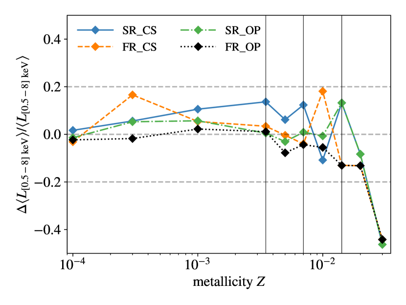
Figure 20: Relative difference between the X-ray luminosities per unit SFR in the $0.5-8$ keV band with $f_{\rm corr}=0.5$ from the two initial condition models defined in Sec. 2.3. In the y axis, the denominator is the result from the default model with a log-flat initial separation distribution, while the nominator is the result from the hybrid initial orbital period distribution (Eqs. 2-4) minus that from the default model. The thin vertical lines label the metallicities of the MW, LMC and SMC (from right to left)

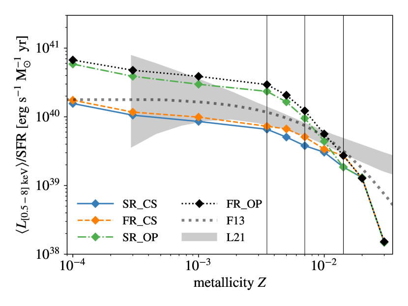
Figure 21: Same as Fig. 14 but comparing the results for the $0.5-8$ keV band from the SR_CS (solid), FR_CS (dashed), SR_OP (dash-dotted) and FR_OP (dotted) models with $f_{\rm corr}=0.5$.

To understand the impact of model parameters on the total X-ray output from Be-XRBs, in Fig. 21 we compare the X-ray luminosity per unit SFR in the $0.5-8$ keV band for all the 4 models in Table 2 with $f_{\rm corr}=0.5$. We find that models with higher initial rotation rates (FR) and VDD densities (OP) produce slightly ($\lesssim 50\%$) and significantly (up to a factor of $\sim 4$) higher X-ray luminosities than in the fiducial case SR_CS, respectively. In the OP models with $f_{\rm corr}=0.5$, the luminosity from Be-XRBs is higher than that observed for all types of HMXBs (Lehmer et al., 2021) by up to a factor of $\sim 2$. This means that the OP models can only be consistent with observations with $f_{\rm corr}\lesssim 0.25$. Indeed, it is shown in 22 that the X-ray luminosity and number of (ultra-)luminous HMXBs per unit SFR from Be-XRBs in the SR_OP model reach the observed values for all types of HMXBs given $f_{\rm corr}=0.25$. Since $f_{\rm corr}=0.25$ is already the lower limit allowed by the calibration of accretion rate/luminosity for Be-XRBs (Sec. 3.2.1), and other types of HMXBs also contribute to the observed luminosity/number, we conclude that the OP models are strongly disfavoured. Similarly, we find that $f_{\rm corr}\gtrsim 0.8$ is ruled out for the CS models, as illustrated in Fig. 23 where the observed X-ray luminosity and number of (ultra-)luminous HMXBs per unit SFR for all types of HMXBs from Lehmer et al. (2021) are reproduced solely by Be-XRBs in the SR_CS model with $f_{\rm corr}=0.8$.

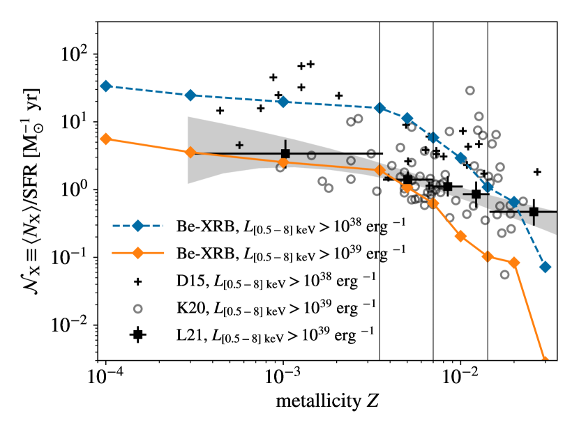
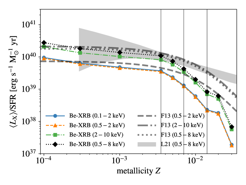
Figure 22: Same as Figs. 8 (top) and 14 (bottom) but for the SR_OP model with a lower correction factor $f_{\rm corr}=0.25$.

Figure 23: Same as Figs. 8 (top) and 14 (bottom) but with a higher correction factor $f_{\rm corr}=0.8$.

References

- Abdusalam et al. (2020) Abdusalam K., Ablimit I., Hashim P., Lü G. L., Mardini M. K., Wang Z. J., 2020, ApJ, 902, 125
- Acharya et al. (2023) Acharya S. K., Cyr B., Chluba J., 2023, MNRAS, 523, 1908
- Aird et al. (2017) Aird J., Coil A. L., Georgakakis A., 2017, MNRAS, 465, 3390
- Allende Prieto et al. (2001) Allende Prieto C., Lambert D. L., Asplund M., 2001, ApJ, 556, L63
- Anastasopoulou et al. (2022) Anastasopoulou K., Zezas A., Steiner J. F., Reig P., 2022, MNRAS, 513, 1400
- Antoniou & Zezas (2016) Antoniou V., Zezas A., 2016, MNRAS, 459, 528
- Antoniou et al. (2009) Antoniou V., Hatzidimitriou D., Zezas A., Reig P., 2009, ApJ, 707, 1080
- Antoniou et al. (2010) Antoniou V., Zezas A., Hatzidimitriou D., Kalogera V., 2010, ApJ, 716, L140
- Antoniou et al. (2019) Antoniou V., et al., 2019, ApJ, 887, 20
- Arcos et al. (2017) Arcos C., Jones C. E., Sigut T. A. A., Kanaan S., Curé M., 2017, ApJ, 842, 48
- Arroyo-Polonio et al. (2023) Arroyo-Polonio J. M., Battaglia G., Thomas G. F., Irwin M. J., McConnachie A. W., Tolstoy E., 2023, A&A, 677, A95
- Artale et al. (2015) Artale M. C., Tissera P. B., Pellizza L. J., 2015, MNRAS, 448, 3071
- Asplund et al. (2004) Asplund M., Grevesse N., Sauval A. J., Allende Prieto C., Kiselman D., 2004, A&A, 417, 751
- Asplund et al. (2009) Asplund M., Grevesse N., Sauval A. J., Scott P., 2009, ARA&A, 47, 481
- Barkana (2018) Barkana R., 2018, Nature, 555, 71
- Bastian et al. (2017) Bastian N., et al., 2017, MNRAS, 465, 4795
- Basu-Zych et al. (2013) Basu-Zych A. R., et al., 2013, ApJ, 762, 45
- Bavera et al. (2020) Bavera S. S., et al., 2020, A&A, 635, A97
- Belczynski & Ziolkowski (2009) Belczynski K., Ziolkowski J., 2009, ApJ, 707, 870
- Bera et al. (2023) Bera A., Samui S., Datta K. K., 2023, MNRAS, 519, 4869
- Bevins et al. (2023) Bevins H. T. J., Heimersheim S., Abril-Cabezas I., Fialkov A., de Lera Acedo E., Handley W., Singh S., Barkana R., 2023, MNRAS,
- Bodensteiner et al. (2020) Bodensteiner J., Shenar T., Sana H., 2020, A&A, 641, A42
- Bowman et al. (2018) Bowman J. D., Rogers A. E. E., Monsalve R. A., Mozdzen T. J., Mahesh N., 2018, Nature, 555, 67
- Brorby et al. (2016) Brorby M., Kaaret P., Prestwich A., Mirabel I. F., 2016, MNRAS, 457, 4081
- Brown et al. (2018) Brown R. O., Ho W. C. G., Coe M. J., Okazaki A. T., 2018, MNRAS, 477, 4810
- Brown et al. (2019) Brown R. O., Coe M. J., Ho W. C. G., Okazaki A. T., 2019, MNRAS, 488, 387
- Cappelluti et al. (2017) Cappelluti N., et al., 2017, ApJ, 837, 19
- Carciofi & Bjorkman (2006) Carciofi A. C., Bjorkman J. E., 2006, ApJ, 639, 1081
- Carciofi & Bjorkman (2008) Carciofi A. C., Bjorkman J. E., 2008, ApJ, 684, 1374
- Casares et al. (2014) Casares J., Negueruela I., Ribó M., Ribas I., Paredes J. M., Herrero A., Simón-Díaz S., 2014, Nature, 505, 378
- Chashkina et al. (2019) Chashkina A., Lipunova G., Abolmasov P., Poutanen J., 2019, A&A, 626, A18
- Chatterjee et al. (2020) Chatterjee A., Dayal P., Choudhury T. R., Schneider R., 2020, MNRAS, 496, 1445
- Cheng et al. (2014) Cheng Z. Q., Shao Y., Li X. D., 2014, ApJ, 786, 128
- Chiappini (2013) Chiappini C., 2013, Astronomische Nachrichten, 334, 595
- Chiappini et al. (2006) Chiappini C., Hirschi R., Meynet G., Ekström S., Maeder A., Matteucci F., 2006, A&A, 449, L27
- Chiappini et al. (2011) Chiappini C., Frischknecht U., Meynet G., Hirschi R., Barbuy B., Pignatari M., Decressin T., Maeder A., 2011, Nature, 472, 454
- Choi et al. (2017) Choi J., Conroy C., Byler N., 2017, ApJ, 838, 159
- Chon et al. (2021) Chon S., Omukai K., Schneider R., 2021, MNRAS, 508, 4175
- Chon et al. (2022) Chon S., Ono H., Omukai K., Schneider R., 2022, MNRAS, 514, 4639
- Choplin et al. (2017) Choplin A., Hirschi R., Meynet G., Ekström S., 2017, A&A, 607, L3
- Choplin et al. (2019) Choplin A., Tominaga N., Ishigaki M. N., 2019, A&A, 632, A62
- Coe & Kirk (2015) Coe M. J., Kirk J., 2015, MNRAS, 452, 969
- Cranmer (2009) Cranmer S. R., 2009, ApJ, 701, 396
- Cyr et al. (2017) Cyr I. H., Jones C. E., Panoglou D., Carciofi A. C., Okazaki A. T., 2017, MNRAS, 471, 596
- Dai et al. (2006) Dai H.-L., Liu X.-W., Li X.-D., 2006, ApJ, 653, 1410
- Dallas et al. (2022) Dallas M. M., Oey M. S., Castro N., 2022, ApJ, 936, 112
- Das et al. (2017) Das A., Mesinger A., Pallottini A., Ferrara A., Wise J. H., 2017, MNRAS, 469, 1166
- Davies et al. (2015) Davies B., Kudritzki R.-P., Gazak Z., Plez B., Bergemann M., Evans C., Patrick L., 2015, ApJ, 806, 21
- DeBoer et al. (2017) DeBoer D. R., et al., 2017, PASP, 129, 045001
- Dodd et al. (2023) Dodd J. M., Oudmaijer R. D., Radley I. C., Vioque M., Frost A. J., 2023, MNRAS,
- Dorigo Jones et al. (2020) Dorigo Jones J., Oey M. S., Paggeot K., Castro N., Moe M., 2020, ApJ, 903, 43
- Douna et al. (2015) Douna V. M., Pellizza L. J., Mirabel I. F., Pedrosa S. E., 2015, A&A, 579, A44
- Drout et al. (2023) Drout M. R., Götberg Y., Ludwig B. A., Groh J. H., de Mink S. E., O’Grady A. J. G., Smith N., 2023, arXiv e-prints, p. arXiv:2307.00061
- Duchêne & Kraus (2013) Duchêne G., Kraus A., 2013, ARA&A, 51, 269
- Eggleton (1983) Eggleton P. P., 1983, ApJ, 268, 368
- Eide et al. (2018) Eide M. B., Graziani L., Ciardi B., Feng Y., Kakiichi K., Di Matteo T., 2018, MNRAS, 476, 1174
- Ekström et al. (2008) Ekström S., Meynet G., Maeder A., Barblan F., 2008, A&A, 478, 467
- Ekström et al. (2012) Ekström S., et al., 2012, A&A, 537, A146
- Ewall-Wice et al. (2018) Ewall-Wice A., Chang T. C., Lazio J., Doré O., Seiffert M., Monsalve R. A., 2018, ApJ, 868, 63
- Fabrika et al. (2021) Fabrika S. N., Atapin K. E., Vinokurov A. S., Sholukhova O. N., 2021, Astrophysical Bulletin, 76, 6
- Farmer et al. (2019) Farmer R., Renzo M., de Mink S. E., Marchant P., Justham S., 2019, ApJ, 887, 53
- Fialkov & Barkana (2014) Fialkov A., Barkana R., 2014, MNRAS, 445, 213
- Fialkov et al. (2013) Fialkov A., Barkana R., Visbal E., Tseliakhovich D., Hirata C. M., 2013, MNRAS, 432, 2909
- Fialkov et al. (2014) Fialkov A., Barkana R., Visbal E., 2014, Nature, 506, 197
- Fialkov et al. (2017) Fialkov A., Cohen A., Barkana R., Silk J., 2017, MNRAS, 464, 3498
- Fishbach & Kalogera (2022) Fishbach M., Kalogera V., 2022, ApJ, 929, L26
- Fornasini et al. (2019) Fornasini F. M., et al., 2019, ApJ, 885, 65
- Fornasini et al. (2020) Fornasini F. M., Civano F., Suh H., 2020, MNRAS, 495, 771
- Fornasini et al. (2023) Fornasini F. M., Antoniou V., Dubus G., 2023, arXiv e-prints, p. arXiv:2308.02645
- Fortin et al. (2023) Fortin F., García F., Simaz Bunzel A., Chaty S., 2023, A&A, 671, A149
- Fragos et al. (2013a) Fragos T., et al., 2013a, ApJ, 764, 41
- Fragos et al. (2013b) Fragos T., Lehmer B. D., Naoz S., Zezas A., Basu-Zych A., 2013b, ApJ, 776, L31
- Franchini & Martin (2021) Franchini A., Martin R. G., 2021, ApJ, 923, L18
- Frost et al. (2022) Frost A. J., et al., 2022, A&A, 659, L3
- Georgy et al. (2013) Georgy C., et al., 2013, A&A, 558, A103
- Gessey-Jones et al. (2022) Gessey-Jones T., et al., 2022, MNRAS, 516, 841
- Gessey-Jones et al. (2023) Gessey-Jones T., Fialkov A., de Lera Acedo E., Handley W. J., Barkana R., 2023, MNRAS, 526, 4262
- Ghara et al. (2022) Ghara R., Mellema G., Zaroubi S., 2022, J. Cosmology Astropart. Phys., 2022, 055
- Gilfanov et al. (2022) Gilfanov M., Fabbiano G., Lehmer B., Zezas A., 2022, in , Handbook of X-ray and Gamma-ray Astrophysics. p. 105, doi:10.1007/978-981-16-4544-0_108-1
- Gotberg et al. (2023) Gotberg Y., et al., 2023, arXiv e-prints, p. arXiv:2307.00074
- Granada et al. (2013) Granada A., Ekström S., Georgy C., Krtička J., Owocki S., Meynet G., Maeder A., 2013, A&A, 553, A25
- Groh et al. (2019) Groh J. H., et al., 2019, A&A, 627, A24
- Grudzinska et al. (2015) Grudzinska M., et al., 2015, MNRAS, 452, 2773
- Gunawardhana et al. (2011) Gunawardhana M. L. P., et al., 2011, MNRAS, 415, 1647
- Haberl & Sturm (2016) Haberl F., Sturm R., 2016, A&A, 586, A81
- Hansen & Phinney (1997) Hansen B. M. S., Phinney E. S., 1997, MNRAS, 291, 569
- Hassan et al. (2023) Hassan S., et al., 2023, arXiv e-prints, p. arXiv:2305.02703
- Hastings et al. (2020) Hastings B., Wang C., Langer N., 2020, A&A, 633, A165
- Hastings et al. (2021) Hastings B., Langer N., Wang C., Schootemeijer A., Milone A. P., 2021, A&A, 653, A144
- Haubois et al. (2012) Haubois X., Carciofi A. C., Rivinius T., Okazaki A. T., Bjorkman J. E., 2012, ApJ, 756, 156
- Hendriks & Izzard (2023a) Hendriks D. D., Izzard R. G., 2023a, Journal of Open Source Software, 8, 4642
- Hendriks & Izzard (2023b) Hendriks D. D., Izzard R. G., 2023b, MNRAS, 524, 4315
- Hendriks et al. (2023) Hendriks D. D., van Son L. A. C., Renzo M., Izzard R. G., Farmer R., 2023, MNRAS, 526, 4130
- Hirano & Bromm (2018) Hirano S., Bromm V., 2018, MNRAS, 476, 3964
- Hohle et al. (2010) Hohle M. M., Neuhäuser R., Schutz B. F., 2010, Astronomische Nachrichten, 331, 349
- Huang (1963) Huang S.-S., 1963, ApJ, 138, 342
- Hummel et al. (2015) Hummel J. A., Stacy A., Jeon M., Oliveri A., Bromm V., 2015, MNRAS, 453, 4136
- Hummel et al. (2016) Hummel J. A., Stacy A., Bromm V., 2016, MNRAS, 460, 2432
- Hunter (2007) Hunter J. D., 2007, Computing in Science and Engineering, 9, 90
- Hurley et al. (2000) Hurley J. R., Pols O. R., Tout C. A., 2000, MNRAS, 315, 543
- Hurley et al. (2002) Hurley J. R., Tout C. A., Pols O. R., 2002, MNRAS, 329, 897
- Igoshev et al. (2021) Igoshev A. P., Chruslinska M., Dorozsmai A., Toonen S., 2021, MNRAS, 508, 3345
- Inayoshi et al. (2017) Inayoshi K., Hirai R., Kinugawa T., Hotokezaka K., 2017, MNRAS, 468, 5020
- Izzard & Halabi (2018) Izzard R. G., Halabi G. M., 2018, arXiv e-prints, p. arXiv:1808.06883
- Izzard & Jermyn (2023) Izzard R. G., Jermyn A. S., 2023, MNRAS, 521, 35
- Izzard et al. (2004) Izzard R. G., Tout C. A., Karakas A. I., Pols O. R., 2004, MNRAS, 350, 407
- Izzard et al. (2006) Izzard R. G., Dray L. M., Karakas A. I., Lugaro M., Tout C. A., 2006, A&A, 460, 565
- Izzard et al. (2009) Izzard R. G., Glebbeek E., Stancliffe R. J., Pols O. R., 2009, A&A, 508, 1359
- Izzard et al. (2017) Izzard R. G., Preece H., Jofre P., Halabi G. M., Masseron T., Tout C. A., 2017, MNRAS, 473, 2984
- Janssens et al. (2023) Janssens S., Shenar T., Degenaar N., Bodensteiner J., Sana H., Audenaert J., Frost A. J., 2023, A&A, 677, L9
- Jeena et al. (2023) Jeena S. K., Banerjee P., Chiaki G., Heger A., 2023, MNRAS, 526, 4467
- Jeon et al. (2012) Jeon M., Pawlik A. H., Greif T. H., Glover S. C. O., Bromm V., Milosavljević M., Klessen R. S., 2012, ApJ, 754, 34
- Jeřábková et al. (2018) Jeřábková T., Hasani Zonoozi A., Kroupa P., Beccari G., Yan Z., Vazdekis A., Zhang Z. Y., 2018, A&A, 620, A39
- Johnson et al. (2013) Johnson J. L., Dalla Vecchia C., Khochfar S., 2013, MNRAS, 428, 1857
- Jones et al. (2001) Jones E., Oliphant T., Peterson P., et al., 2001
- Kaaret et al. (2017) Kaaret P., Feng H., Roberts T. P., 2017, ARA&A, 55, 303
- Kamran et al. (2022) Kamran M., Ghara R., Majumdar S., Mellema G., Bharadwaj S., Pritchard J. R., Mondal R., Iliev I. T., 2022, J. Cosmology Astropart. Phys., 2022, 001
- Karino (2022) Karino S., 2022, MNRAS, 514, 191
- Kaur et al. (2022) Kaur H. D., Qin Y., Mesinger A., Pallottini A., Fragos T., Basu-Zych A., 2022, MNRAS, 513, 5097
- Kennea et al. (2021) Kennea J. A., Coe M. J., Evans P. A., Townsend L. J., Campbell Z. A., Udalski A., 2021, MNRAS, 508, 781
- Khan et al. (2022) Khan N., Middleton M. J., Wiktorowicz G., Dauser T., Roberts T. P., Wilms J., 2022, MNRAS, 509, 2493
- Khokhlov et al. (2018) Khokhlov S. A., et al., 2018, ApJ, 856, 158
- King (2009) King A. R., 2009, MNRAS, 393, L41
- King et al. (2001) King A. R., Davies M. B., Ward M. J., Fabbiano G., Elvis M., 2001, ApJ, 552, L109
- King et al. (2023) King A., Lasota J.-P., Middleton M., 2023, New Astron. Rev., 96, 101672
- Klement et al. (2017) Klement R., et al., 2017, A&A, 601, A74
- Klement et al. (2019) Klement R., et al., 2019, ApJ, 885, 147
- Koopmans et al. (2015) Koopmans L., et al., 2015, in Advancing Astrophysics with the Square Kilometre Array (AASKA14). p. 1 (arXiv:1505.07568), doi:10.22323/1.215.0001
- Kotko & Belczynski (2023) Kotko I., Belczynski K., 2023, arXiv e-prints, p. arXiv:2305.08640
- Kovlakas et al. (2020) Kovlakas K., Zezas A., Andrews J. J., Basu-Zych A., Fragos T., Hornschemeier A., Lehmer B., Ptak A., 2020, MNRAS, 498, 4790
- Kovlakas et al. (2022) Kovlakas K., Fragos T., Schaerer D., Mesinger A., 2022, A&A, 665, A28
- Kretschmar et al. (2019) Kretschmar P., et al., 2019, New Astron. Rev., 86, 101546
- Kroupa (1995) Kroupa P., 1995, MNRAS, 277, 1507
- Kroupa (2001) Kroupa P., 2001, MNRAS, 322, 231
- Krtička et al. (2011) Krtička J., Owocki S. P., Meynet G., 2011, A&A, 527, A84
- Krtička et al. (2015) Krtička J., Kurfürst P., Krtičková I., 2015, A&A, 573, A20
- Kulkarni et al. (2021) Kulkarni M., Visbal E., Bryan G. L., 2021, ApJ, 917, 40
- Kuranov et al. (2020) Kuranov A. G., Postnov K. A., Yungelson L. R., 2020, Astronomy Letters, 46, 658
- Lacchin et al. (2020) Lacchin E., Matteucci F., Vincenzo F., Palla M., 2020, MNRAS, 495, 3276
- Lang (1992) Lang K. R., 1992, Astrophysical Data. Springer-Verlag
- Lasota & King (2023) Lasota J.-P., King A., 2023, MNRAS, 526, 2506
- Lazare et al. (2023) Lazare H., Sarkar D., Kovetz E. D., 2023, arXiv e-prints, p. arXiv:2307.15577
- Lazzarini et al. (2023) Lazzarini M., et al., 2023, ApJ, 952, 114
- Lee et al. (2014) Lee U., Neiner C., Mathis S., 2014, MNRAS, 443, 1515
- Lehmer et al. (2012) Lehmer B. D., et al., 2012, ApJ, 752, 46
- Lehmer et al. (2016) Lehmer B. D., et al., 2016, ApJ, 825, 7
- Lehmer et al. (2019) Lehmer B. D., et al., 2019, ApJS, 243, 3
- Lehmer et al. (2021) Lehmer B. D., et al., 2021, ApJ, 907, 17
- Lehmer et al. (2022) Lehmer B. D., Eufrasio R. T., Basu-Zych A., Garofali K., Gilbertson W., Mesinger A., Yukita M., 2022, ApJ, 930, 135
- Lewis et al. (2023) Lewis J. S. W., Pillepich A., Nelson D., Klessen R. S., Glover S. C. O., 2023, arXiv e-prints, p. arXiv:2305.09721
- Linden et al. (2009) Linden T., Sepinsky J. F., Kalogera V., Belczynski K., 2009, ApJ, 699, 1573
- Linden et al. (2010) Linden T., Kalogera V., Sepinsky J. F., Prestwich A., Zezas A., Gallagher J. S., 2010, ApJ, 725, 1984
- Liotine et al. (2023) Liotine C., Zevin M., Berry C. P. L., Doctor Z., Kalogera V., 2023, ApJ, 946, 4
- Liu & Bromm (2020) Liu B., Bromm V., 2020, MNRAS, 497, 2839
- Liu et al. (2019) Liu B., Schauer A. T. P., Bromm V., 2019, MNRAS, 487, 4711
- Liu et al. (2021) Liu B., Meynet G., Bromm V., 2021, MNRAS, 501, 643
- Lodato & Price (2010) Lodato G., Price D. J., 2010, MNRAS, 405, 1212
- Ma et al. (2018) Ma Q., Ciardi B., Eide M. B., Helgason K., 2018, MNRAS, 480, 26
- Ma et al. (2023) Ma Q.-B., Ghara R., Ciardi B., Iliev I. T., Koopmans L. V. E., Mellema G., Mondal R., Zaroubi S., 2023, MNRAS, 522, 3284
- Madau (2018) Madau P., 2018, MNRAS, 480, L43
- Madau & Fragos (2017) Madau P., Fragos T., 2017, ApJ, 840, 39
- Maeder et al. (2015) Maeder A., Meynet G., Chiappini C., 2015, A&A, 576, A56
- Magg et al. (2022) Magg M., et al., 2022, MNRAS, 514, 4433
- Mapelli et al. (2010) Mapelli M., Ripamonti E., Zampieri L., Colpi M., Bressan A., 2010, MNRAS, 408, 234
- Maravelias et al. (2014) Maravelias G., Zezas A., Antoniou V., Hatzidimitriou D., 2014, MNRAS, 438, 2005
- Marchant et al. (2017) Marchant P., Langer N., Podsiadlowski P., Tauris T. M., de Mink S., Mandel I., Moriya T. J., 2017, A&A, 604, A55
- Marks et al. (2012) Marks M., Kroupa P., Dabringhausen J., Pawlowski M. S., 2012, MNRAS, 422, 2246
- Martin et al. (2011) Martin R. G., Pringle J. E., Tout C. A., Lubow S. H., 2011, MNRAS, 416, 2827
- McClintock & Remillard (2006) McClintock J. E., Remillard R. A., 2006, in , Vol. 39, Compact stellar X-ray sources. pp 157–213
- Mertens et al. (2021) Mertens F. G., Semelin B., Koopmans L. V. E., 2021, in Siebert A., et al., eds, SF2A-2021: Proceedings of the Annual meeting of the French Society of Astronomy and Astrophysics. pp 211–214 (arXiv:2109.10055), doi:10.48550/arXiv.2109.10055
- Mineo et al. (2012) Mineo S., Gilfanov M., Sunyaev R., 2012, MNRAS, 419, 2095
- Mirocha & Furlanetto (2019) Mirocha J., Furlanetto S. R., 2019, MNRAS, 483, 1980
- Mirouh et al. (2023) Mirouh G. M., Hendriks D. D., Dykes S., Moe M., Izzard R. G., 2023, MNRAS, 524, 3978
- Misra et al. (2020) Misra D., Fragos T., Tauris T. M., Zapartas E., Aguilera-Dena D. R., 2020, A&A, 642, A174
- Misra et al. (2023a) Misra D., et al., 2023a, arXiv e-prints, p. arXiv:2309.15904
- Misra et al. (2023b) Misra D., et al., 2023b, A&A, 672, A99
- Moe & Di Stefano (2017) Moe M., Di Stefano R., 2017, ApJS, 230, 15
- Moe et al. (2019) Moe M., Kratter K. M., Badenes C., 2019, ApJ, 875, 61
- Mondal & Barkana (2023) Mondal R., Barkana R., 2023, Nature Astronomy, 7, 1025
- Mondal et al. (2020) Mondal S., Belczyński K., Wiktorowicz G., Lasota J.-P., King A. R., 2020, MNRAS, 491, 2747
- Mondal et al. (2023) Mondal R., Barkana R., Fialkov A., 2023, arXiv e-prints, p. arXiv:2310.15530
- Monsalve et al. (2023) Monsalve R. A., et al., 2023, arXiv e-prints, p. arXiv:2309.02996
- Montero-Camacho et al. (2023) Montero-Camacho P., Zhang Y., Mao Y., 2023, arXiv e-prints, p. arXiv:2307.10598
- Moretti et al. (2012) Moretti A., Vattakunnel S., Tozzi P., Salvaterra R., Severgnini P., Fugazza D., Haardt F., Gilli R., 2012, A&A, 548, A87
- Muñoz et al. (2022) Muñoz J. B., Qin Y., Mesinger A., Murray S. G., Greig B., Mason C., 2022, MNRAS, 511, 3657
- Munar-Adrover et al. (2014) Munar-Adrover P., Paredes J. M., Ribó M., Iwasawa K., Zabalza V., Casares J., 2014, ApJ, 786, L11
- Murphy et al. (2021) Murphy L. J., et al., 2021, MNRAS, 501, 2745
- Mushtukov & Portegies Zwart (2023) Mushtukov A. A., Portegies Zwart S., 2023, MNRAS, 518, 5457
- Mushtukov & Tsygankov (2022) Mushtukov A., Tsygankov S., 2022, arXiv e-prints, p. arXiv:2204.14185
- Nixon & Pringle (2020) Nixon C. J., Pringle J. E., 2020, ApJ, 905, L29
- Ogilvie (1999) Ogilvie G. I., 1999, MNRAS, 304, 557
- Okazaki (2001) Okazaki A. T., 2001, PASJ, 53, 119
- Okazaki & Negueruela (2001) Okazaki A. T., Negueruela I., 2001, A&A, 377, 161
- Okazaki et al. (2002) Okazaki A. T., Bate M. R., Ogilvie G. I., Pringle J. E., 2002, MNRAS, 337, 967
- Okazaki et al. (2013) Okazaki A. T., Hayasaki K., Moritani Y., 2013, PASJ, 65, 41
- Pacucci et al. (2014) Pacucci F., Mesinger A., Mineo S., Ferrara A., 2014, MNRAS, 443, 678
- Paczyński & Sienkiewicz (1972) Paczyński B., Sienkiewicz R., 1972, Acta Astron., 22, 73
- Pallottini et al. (2014) Pallottini A., Ferrara A., Gallerani S., Salvadori S., D’Odorico V., 2014, MNRAS, 440, 2498
- Panoglou et al. (2016) Panoglou D., Carciofi A. C., Vieira R. G., Cyr I. H., Jones C. E., Okazaki A. T., Rivinius T., 2016, MNRAS, 461, 2616
- Panoglou et al. (2018) Panoglou D., Faes D. M., Carciofi A. C., Okazaki A. T., Baade D., Rivinius T., Borges Fernandes M., 2018, MNRAS, 473, 3039
- Park et al. (2021a) Park J., Ricotti M., Sugimura K., 2021a, MNRAS, 508, 6176
- Park et al. (2021b) Park J., Ricotti M., Sugimura K., 2021b, MNRAS, 508, 6193
- Park et al. (2023a) Park J., Ricotti M., Sugimura K., 2023a, arXiv e-prints, p. arXiv:2307.14562
- Park et al. (2023b) Park J., Ricotti M., Sugimura K., 2023b, MNRAS, 521, 5334
- Paxton et al. (2018) Paxton B., et al., 2018, ApJS, 234, 34
- Paxton et al. (2019) Paxton B., et al., 2019, ApJS, 243, 10
- Pradhan et al. (2021) Pradhan P., Paul B., Bozzo E., Maitra C., Paul B. C., 2021, MNRAS, 502, 1163
- Prestwich et al. (2013) Prestwich A. H., Tsantaki M., Zezas A., Jackson F., Roberts T. P., Foltz R., Linden T., Kalogera V., 2013, ApJ, 769, 92
- Pringle (1981) Pringle J. E., 1981, ARA&A, 19, 137
- Pritchard & Furlanetto (2007) Pritchard J. R., Furlanetto S. R., 2007, MNRAS, 376, 1680
- Qiao & Liu (2020) Qiao E., Liu B. F., 2020, MNRAS, 492, 615
- Qin et al. (2020) Qin Y., Mesinger A., Park J., Greig B., Muñoz J. B., 2020, MNRAS, 495, 123
- Raguzova & Popov (2005) Raguzova N. V., Popov S. B., 2005, Astronomical and Astrophysical Transactions, 24, 151
- Ramachandran et al. (2023) Ramachandran V., Klencki J., Sander A. A. C., Pauli D., Shenar T., Oskinova L. M., Hamann W. R., 2023, A&A, 674, L12
- Reig (2011) Reig P., 2011, Ap&SS, 332, 1
- Reis et al. (2021) Reis I., Fialkov A., Barkana R., 2021, MNRAS, 506, 5479
- Ressler (2021) Ressler S. M., 2021, MNRAS, 508, 4887
- Riccio et al. (2023) Riccio G., et al., 2023, A&A, 678, A164
- Richardson et al. (2023) Richardson N. D., et al., 2023, Nature, 614, 45
- Ricotti (2016) Ricotti M., 2016, MNRAS, 462, 601
- Riley et al. (2022) Riley J., et al., 2022, ApJS, 258, 34
- Rímulo et al. (2018) Rímulo L. R., et al., 2018, MNRAS, 476, 3555
- Rivinius (2019) Rivinius T., 2019, IAU Symposium, 346, 105
- Rivinius et al. (2013) Rivinius T., Carciofi A. C., Martayan C., 2013, A&ARv, 21, 69
- Rogers et al. (2013) Rogers T. M., Lin D. N. C., McElwaine J. N., Lau H. H. B., 2013, ApJ, 772, 21
- Rossland et al. (2023) Rossland S., et al., 2023, AJ, 166, 20
- Rubele et al. (2015) Rubele S., et al., 2015, MNRAS, 449, 639
- Rusakov et al. (2023) Rusakov V., Steinhardt C. L., Sneppen A., 2023, ApJS, 268, 10
- Safranek-Shrader et al. (2012) Safranek-Shrader C., Agarwal M., Federrath C., Dubey A., Milosavljević M., Bromm V., 2012, MNRAS, 426, 1159
- Salvaggio et al. (2023) Salvaggio C., Wolter A., Belfiore A., Colpi M., 2023, MNRAS, 522, 1377
- Sana et al. (2012) Sana H., et al., 2012, Science, 337, 444
- Sander & Vink (2020) Sander A. A. C., Vink J. S., 2020, MNRAS, 499, 873
- Sartorio et al. (2023) Sartorio N. S., et al., 2023, MNRAS,
- Schauer et al. (2019) Schauer A. T. P., Liu B., Bromm V., 2019, ApJ, 877, L5
- Schauer et al. (2021) Schauer A. T. P., Glover S. C. O., Klessen R. S., Clark P., 2021, MNRAS, 507, 1775
- Schmidtke et al. (2013) Schmidtke P. C., Cowley A. P., Udalski A., 2013, MNRAS, 431, 252
- Schneider et al. (2018) Schneider F. R. N., et al., 2018, Science, 359, 69
- Schootemeijer et al. (2022) Schootemeijer A., Lennon D. J., Garcia M., Langer N., Hastings B., Schürmann C., 2022, A&A, 667, A100
- Sguera et al. (2023) Sguera V., Sidoli L., Bird A. J., La Palombara N., 2023, MNRAS, 523, 1192
- Shakura & Sunyaev (1973) Shakura N. I., Sunyaev R. A., 1973, A&A, 24, 337
- Shao & Li (2014) Shao Y., Li X.-D., 2014, ApJ, 796, 37
- Shao & Li (2020) Shao Y., Li X.-D., 2020, ApJ, 898, 143
- Shao et al. (2019) Shao Y., Li X.-D., Dai Z.-G., 2019, ApJ, 886, 118
- Shao et al. (2023) Shao Y., Xu Y., Wang Y., Yang W., Li R., Zhang X., Chen X., 2023, Nature Astronomy,
- Sidoli & Paizis (2018) Sidoli L., Paizis A., 2018, MNRAS, 481, 2779
- Singh et al. (2022) Singh S., et al., 2022, Nature Astronomy, 6, 607
- Soberman et al. (1997) Soberman G. E., Phinney E. S., van den Heuvel E. P. J., 1997, A&A, 327, 620
- Sokolova-Lapa et al. (2021) Sokolova-Lapa E., et al., 2021, A&A, 651, A12
- Stacy & Bromm (2007) Stacy A., Bromm V., 2007, MNRAS, 382, 229
- Stacy et al. (2011) Stacy A., Bromm V., Loeb A., 2011, MNRAS, 413, 543
- Stacy et al. (2013) Stacy A., Greif T. H., Klessen R. S., Bromm V., Loeb A., 2013, MNRAS, 431, 1470
- Steiner et al. (2009) Steiner J. F., Narayan R., McClintock J. E., Ebisawa K., 2009, PASP, 121, 1279
- Suffak et al. (2022) Suffak M., Jones C. E., Carciofi A. C., 2022, MNRAS, 509, 931
- Sugimura et al. (2020) Sugimura K., Matsumoto T., Hosokawa T., Hirano S., Omukai K., 2020, ApJ, 892, L14
- Sugimura et al. (2023) Sugimura K., Matsumoto T., Hosokawa T., Hirano S., Omukai K., 2023, arXiv e-prints, p. arXiv:2307.15108
- Takhistov et al. (2022) Takhistov V., Lu P., Gelmini G. B., Hayashi K., Inoue Y., Kusenko A., 2022, J. Cosmology Astropart. Phys., 2022, 017
- Tanvir & Krumholz (2023) Tanvir T. S., Krumholz M. R., 2023, arXiv e-prints, p. arXiv:2305.20039
- Tranin et al. (2023) Tranin H., Webb N., Godet O., 2023, arXiv e-prints, p. arXiv:2304.11216
- Ucci et al. (2023) Ucci G., et al., 2023, MNRAS, 518, 3557
- Ventura et al. (2023) Ventura E. M., Trinca A., Schneider R., Graziani L., Valiante R., Wyithe J. S. B., 2023, MNRAS,
- Verbunt et al. (2017) Verbunt F., Igoshev A., Cator E., 2017, A&A, 608, A57
- Vieira et al. (2017) Vieira R. G., Carciofi A. C., Bjorkman J. E., Rivinius T., Baade D., Rímulo L. R., 2017, MNRAS, 464, 3071
- Vigna-Gómez et al. (2018) Vigna-Gómez A., et al., 2018, MNRAS, 481, 4009
- Vinciguerra et al. (2020) Vinciguerra S., et al., 2020, MNRAS, 498, 4705
- Walter et al. (2015) Walter R., Lutovinov A. A., Bozzo E., Tsygankov S. S., 2015, A&ARv, 23, 2
- Walton et al. (2022) Walton D. J., Mackenzie A. D. A., Gully H., Patel N. R., Roberts T. P., Earnshaw H. P., Mateos S., 2022, MNRAS, 509, 1587
- Wang et al. (2023) Wang C., et al., 2023, A&A, 670, A43
- Wiktorowicz et al. (2017) Wiktorowicz G., Sobolewska M., Lasota J.-P., Belczynski K., 2017, ApJ, 846, 17
- Wiktorowicz et al. (2019) Wiktorowicz G., Lasota J.-P., Middleton M., Belczynski K., 2019, ApJ, 875, 53
- Wiktorowicz et al. (2021) Wiktorowicz G., Lasota J.-P., Belczynski K., Lu Y., Liu J., Iłkiewicz K., 2021, ApJ, 918, 60
- Willcox et al. (2023) Willcox R., MacLeod M., Mandel I., Hirai R., 2023, arXiv e-prints, p. arXiv:2308.06666
- Wise et al. (2012) Wise J. H., Turk M. J., Norman M. L., Abel T., 2012, ApJ, 745, 50
- Wood et al. (1997) Wood K., Bjorkman K. S., Bjorkman J. E., 1997, ApJ, 477, 926
- Wu et al. (2010) Wu Y. X., Yu W., Li T. P., Maccarone T. J., Li X. D., 2010, ApJ, 718, 620
- Xing & Li (2021) Xing Z.-P., Li X.-D., 2021, ApJ, 920, 67
- Xu & Li (2019) Xu X.-T., Li X.-D., 2019, ApJ, 872, 102
- Xu et al. (2013) Xu H., Wise J. H., Norman M. L., 2013, ApJ, 773, 83
- Yang (2021) Yang Y., 2021, MNRAS, 508, 5709
- Yang et al. (2017) Yang J., Laycock S. G. T., Christodoulou D. M., Fingerman S., Coe M. J., Drake J. J., 2017, ApJ, 839, 119
- Yang et al. (2023) Yang Y., Li X., Li G., 2023, Phys. Rev. D, 107, 103501
- Yates et al. (2023) Yates R. M., Hendriks D., Vijayan A. P., Izzard R. G., Thomas P. A., Das P., 2023, arXiv e-prints, p. arXiv:2310.15218
- Zamanov et al. (2022) Zamanov R. K., et al., 2022, Astronomische Nachrichten, 343, e24019
- Zhang et al. (2004) Zhang F., Li X. D., Wang Z. R., 2004, ApJ, 603, 663
- Zhao & Fuller (2020) Zhao X., Fuller J., 2020, MNRAS, 495, 249
- Zhao et al. (2023) Zhao Y., Gandhi P., Brown C. D., Knigge C., Charles P. A., Maccarone T. J., Nuchvanichakul P., 2023, MNRAS,
- Zuo et al. (2014) Zuo Z.-Y., Li X.-D., Gu Q.-S., 2014, MNRAS, 437, 1187
- de Lera Acedo et al. (2022) de Lera Acedo E., et al., 2022, Nature Astronomy, 6, 984
- van der Walt et al. (2011) van der Walt S., Colbert S. C., Varoquaux G., 2011, Computing in Science and Engineering, 13, 22