Simplified and Improved Bounds on the VC-Dimension for Elastic Distance Measures

Abstract

We study range spaces, where the ground set consists of either polygonal curves in $\mathbb{R}^{d}$ or polygonal regions in the plane that may contain holes and the ranges are balls defined by an elastic distance measure, such as the Hausdorff distance, the Fréchet distance and the dynamic time warping distance. These range spaces appear in various applications like classification, range counting, density estimation and clustering when the instances are trajectories, time series or polygons. The Vapnik–Chervonenkis dimension (VC-dimension) plays an important role when designing algorithms for these range spaces. We show for the Fréchet distance of polygonal curves and the Hausdorff distance of polygonal curves and planar polygonal regions that the VC-dimension is upper-bounded by $O(dk\log(km))$, where $k$ is the complexity of the center of a ball, $m$ is the complexity of the polygonal curve or region in the ground set, and $d$ is the ambient dimension. For $d\geq 4$ this bound is tight in each of the parameters $d,k$ and $m$ separately. For the dynamic time warping distance of polygonal curves, our analysis directly yields an upper-bound of $O(\min(dk^{2}\log(m),dkm\log(k)))$.

1 Introduction

The Vapnik–Chervonenkis dimension (VC-dimension) is a measure of complexity for range spaces that is named after Vladimir Vapnik and Alexey Chervonenkis, who introduced the concept in their seminal paper [21]. Knowing the VC-dimension of a range space can be used to determine sample bounds for various computational tasks. These include sample bounds on the test error of a classification model in statistical learning theory [20] or sample bounds for an $\varepsilon$-net [15] or an $(\eta,\varepsilon)$-approximation [14] in computational geometry. Sample bounds based on the VC-dimension have been successfully applied in the context of kernel density estimation [16], neural networks [3, 17], coresets [6, 10, 11], clustering [2, 5], object recognition [18, 19] and other data analysis tasks.

We study range spaces, where the ground set consists of polygonal curves or polygonal regions and the ranges consist of balls defined by the Hausdorff distance. Previous to our work, Driemel, Nusser, Philips and Psarros [9] derived almost tight bounds on the VC-dimension in the setting of polygonal curves. At the heart of their approach lies the definition of a set of boolean functions (predicates) which are based on the inclusion and intersection of simple geometric objects. The predicates depend on the vertices of a center curve and a radius that defines a metric ball as well as the vertices of a query curve. The predicates are chosen such that, based on their truth values, one can determine whether the query curve is contained in the respective ball. Their proof of the VC-dimension bound uses the worst-case number of operations needed to determine the truth values of each predicate.

In this paper, we extend the known set of predicates to be able to decide the Hausdorff distance between polygonal regions with holes in the plane. We give an improved analysis for the VC-dimension that considers each predicate as a combination of sign values of polynomials. This approach does not use the computational complexity of the distance evaluation, but instead uses the underlying structure of the range space defined by a system of polynomials directly. Our techniques extend to other elastic distance measures, such as the Fréchet distance and the dynamic time warping distance (DTW). By the lower bounds in [9], this approach directly leads to tight bounds for $d\geq 4$ for polygonal curves.

Independent and parallel to our work, Cheng and Huang [7, 8] show the same upper bound of $O(dk\log(km))$ for the Fréchet distance of polygonal curves using very similar techniques, also using sign values of polynomials. Our new upper bounds for the Hausdorff distance of polygonal regions are obtained by an intricate analysis of a new set of predicates which encode the geometry of the polygonal regions with holes.

1.1 Preliminaries

Let $X$ be a set. We call a set ${\mathcal{R}}$ where any $r\in{\mathcal{R}}$ is of the form $r\subseteq X$ a range space with ground set $X$. We say a subset $A\subseteq X$ is shattered by ${\mathcal{R}}$ if for any $A^{\prime}\subseteq A$ there exists an $r\in{\mathcal{R}}$ such that $A^{\prime}=r\cap A$. The VC-dimension of ${\mathcal{R}}$ (denoted by $VCdim({\mathcal{R}})$) is the maximal size of a set $A\subseteq X$ that is shattered by ${\mathcal{R}}$. We define the ball with radius $\Delta$ and center $c$ under the distance measure $d_{\rho}$ on a set $X$ as

$$b_{\rho}(c,\Delta)=\{x\in X\;|\;d_{\rho}(x,c)\leq\Delta\}.$$

We study range spaces with ground set $({\mathbb{R}}^{d})^{m}$ of the form

$${\mathcal{R}}_{\rho,k}=\{b_{\rho}(c,r)\;|\;\Delta\in{\mathbb{R}}_{+},\Delta>0,c\in({\mathbb{R}}^{d})^{k}\}.$$

We call $({\mathbb{R}}^{d})^{k}$ the center set of ${\mathcal{R}}_{\rho,k}$. Let ${\mathcal{R}}$ be a range space with ground set $X$, and $F$ be a class of real-valued functions defined on ${\mathbb{R}}^{d}\times X$. For $a\in{\mathbb{R}}$ let $\textit{{sgn(a)}}=1$ if $a\geq 0$ and $\textit{{sgn(a)}}=0$ if $a<0$. We say that ${\mathcal{R}}$ is a $t$-combination of $sgn(F)$ if there is a boolean function $g:\{0,1\}^{t}\rightarrow\{0,1\}$ and functions $f_{1},\dots,f_{t}\in F$ such that for all $r\in{\mathcal{R}}$ there is a parameter vector $y\in{\mathbb{R}}^{d}$ such that

$$r=\{x\in X\;|\;g(sgn(f_{1}(y,x)),\dots,sgn(f_{t}(y,x)))=1\}.$$

Central to our approach is the following well-known theorem [3] for bounding the VC-dimension of such range spaces. The theorem can be proven by investigating the complexity of arrangements of zero sets of polynomials. The idea goes back to Goldberg and Jerrum [12] and, independently, Ben-David and Lindenbaum [4]. For the sake of completeness, we include a proof of Theorem 1.1 in Section 6.

Theorem 1.1 ([3], Theorem 8.3).

Let $F$ be a class of functions mapping from ${\mathbb{R}}^{d}\times X$ to ${\mathbb{R}}$ so that, for all $x\in X$ and $f\in F$ the function $y\rightarrow f(y,x)$ is a polynomial on ${\mathbb{R}}^{d}$ of degree no more than $l$. Suppose that ${\mathcal{R}}$ is a $t$-combination of $sgn(F)$. Then we have

$$VCdim({\mathcal{R}})\leq 2{d}\log_{2}(12tl).$$

Let $\lVert\cdot\rVert$ denote the standard Euclidean norm. Let $X,Y\subseteq{\mathbb{R}}^{d}$ for some ${d}\in{\mathbb{N}}$. The directed Hausdorff distance from $X$ to $Y$ is defined as

$$d_{\overrightarrow{H}}(X,Y)=\sup_{x\in X}\inf_{y\in Y}\lVert x-y\rVert$$

and the Hausdorff distance between $X$ and $Y$ is defined as

$$d_{H}(X,Y)=\max\{d_{\overrightarrow{H}}(X,Y),d_{\overrightarrow{H}}(Y,X)\}.$$

Let ${d},{m}\in{\mathbb{N}}$. A sequence of vertices $p_{1},\dots,p_{m}\in{\mathbb{R}}^{d}$ defines a polygonal curve $P$ by concatenating consecutive vertices to create the edges $\overline{p_{1},p_{2}},\dots,\overline{p_{{m}-1},p_{m}}$. We may think of $P$ as an element of ${\mathbb{X}}^{d}_{m}\coloneqq({\mathbb{R}}^{d})^{m}$ and write $P\in{\mathbb{X}}^{d}_{m}$. We may also think of $P$ as a continuous function $P:[0,1]\rightarrow{\mathbb{R}}^{d}$ by fixing $m$ values $0=t_{1}<\ldots<t_{m}=1$, and defining $P(t)=\lambda p_{i+1}+(1-\lambda)p_{i}$ where $\lambda=\frac{t-t_{i}}{t_{i+1}-t_{i}}$ for $t_{i}\leq t\leq t_{i+1}$. We call $P$ a closed curve if $p_{1}=p_{m}$ and we call $P$ self-intersecting if there exist $s\in[0,1]$, $t\in(0,1)$ with $s\neq t$ such that $P(s)=P(t)$. In the case that $P$ is a closed curve which is not self-intersecting, we call the union of $P$ with its interior a simple polygonal region $S$ (without holes). We denote with $\partial S$ the boundary of $S$, which is $P$. Given a simple polygonal region $S_{0}$ and a set of disjoint simple polygonal regions $S_{1},\dots,S_{h}$ in the interior of $S_{0}$, we also consider the set $S=S_{0}-\{S_{1}\cup\dots\cup S_{h}\}$ a polygonal region and we call $S_{1},\dots,S_{h}$ the holes of $S$.

For $m_{1},m_{2}\in{\mathbb{N}}$, each sequence $(1,1)=(i_{1},j_{1}),(i_{2},j_{2}),\dots,(i_{M},j_{M})=(m_{1},m_{2})$ such that $i_{k}-i_{k-1}$ and $j_{k}-j_{k-1}$ are either $0$ or $1$ for all $k$ is a warping path from $(1,1)$ to $(m_{1},m_{2})$. We denote with ${\mathcal{W}}_{m_{1},m_{2}}$ the set of all warping paths from $(1,1)$ to $(m_{1},m_{2})$. For any two polygonal curves $P\in{\mathbb{X}}_{m_{1}}^{d}$ with vertices $p_{1},\dots,p_{m_{1}}$ and $Q\in{\mathbb{X}}_{m_{2}}^{d}$ with vertices $q_{1},\dots,q_{m_{2}}$, we also write ${\mathcal{W}}_{P,Q}={\mathcal{W}}_{m_{1},m_{2}}$, and call elements of ${\mathcal{W}}_{P,Q}$ warping paths between $P$ and $Q$. The dynamic time warping distance between $P$ and $Q$ is defined as

$$d_{DTW}(P,Q)=\min_{w\in{\mathcal{W}}_{P,Q}}\sum_{(i,j)\in w}\lVert p_{i}-q_{j}\rVert^{2}.$$

A warping path that attains the above minimum is also called an optimal warping path between $P$ and $Q$. We denote with ${\mathcal{W}}_{m_{1},m_{2}}^{*}\subset{\mathcal{W}}_{m_{1},m_{2}}$ the set of warping paths $w$ such that there exist polygonal curves $P\in{\mathbb{X}}_{m_{1}}^{d}$ and $Q\in{\mathbb{X}}_{m_{2}}^{d}$ with this optimum warping path $w$.

The discrete Fréchet distance of two polygonal curves $P\in{\mathbb{X}}_{m_{1}}^{d}$ with vertices $p_{1},\dots,p_{m_{1}}$ and $Q\in{\mathbb{X}}_{m_{2}}^{d}$ with vertices $q_{1},\dots,q_{m_{2}}$ is defined as

$$d_{\textit{d}F}(P,Q)=\min_{w\in{\mathcal{W}}_{P,Q}}\max_{(i,j)\in w}\lVert p_{i}-q_{j}\rVert.$$

In the continuous case, we define the Fréchet distance of $P$ and $Q$ as

$$d_{F}(P,Q)=\inf_{\alpha,\beta:[0,1]\rightarrow[0,1]}\sup_{t\in[0,1]}\|P(\alpha(t))-Q(\beta(t))\|,$$

where $\alpha$ and $\beta$ range over all functions that are non-decreasing, surjective and continuous. We further define their weak Fréchet distance as

$$d_{\textit{w}F}(P,Q)=\inf_{\alpha,\beta:[0,1]\rightarrow[0,1]}\sup_{t\in[0,1]}\|P(\alpha(t))-Q(\beta(t))\|,$$

where $\alpha$ and $\beta$ range over all continuous functions with $\alpha(0)=\beta(0)=0$ and $\alpha(1)=\beta(1)=1$.

To bound the VC-dimension in the case of polygonal regions which may contain holes, we will use properties of the Voronoi diagram of a set of line segments in the plane. Let $X$ be a set of subsets (called sites) of ${\mathbb{R}}^{2}$. The Voronoi region $reg(A)$ of a site $A\in X$ consists of all points $p\in{\mathbb{R}}^{2}$ for which $A$ is the closest among all sites in $X$, i.e.

$$reg(A)=\{p\in{\mathbb{R}}^{2}\;|\;d_{\overrightarrow{H}}(p,A)<d_{\overrightarrow{H}}(p,B)\;\text{for all}\;B\in X\}.$$

The Voronoi diagram is the complement of the union of all regions $reg(A)$ with $A\in X$, so

$$vd(X)={\mathbb{R}}^{2}\setminus\cup_{A\in X}reg(A).$$

For any two sites $A,B\in X$, we call the set

$$bisec(A,B)=\{p\in{\mathbb{R}}^{2}\;|\;d_{\overrightarrow{H}}(p,A)=d_{\overrightarrow{H}}(p,B)\}$$

the bisector of $A$ and $B$. The Voronoi edge of $A,B\in X$ is defined as

$$ve(A,B)=vd(X)\cap bisec(A,B)$$

and the Voronoi vertices of $A,B,C\in X$ are defined as

$$vv(A,B,C)=vd(X)\cap bisec(A,B)\cap bisec(B,C).$$

2 Results

We derive new bounds on the VC-dimension for range spaces of the form ${\mathcal{R}}_{\rho,k}$ for some distance measure $d_{\rho}$ with a ground set ${\mathbb{R}}_{m}^{d}$ consisting of polygonal curves or polygonal regions that may contain holes. To this end, we write each range as a combination of sign values of polynomials with constant degree and apply Theorem 1.1. More precisely, we take predicates that determine if a curve $P\in{\mathbb{X}}_{m}^{d}$ is in a fixed range $r\in{\mathcal{R}}_{\rho,k}$ and show that each such predicate can be written as a combination of sign values of polynomials with constant degree.

For the Hausdorff distance of polygonal regions (with holes) in the plane, we show that the VC-dimension of ${\mathcal{R}}_{\rho,k}$ is bounded by $O(k\log(km))$. Interestingly, this bound is independent of the number of holes. To the best of our knowledge this is the first non-trivial bound for the Hausdorff distance of polygonal regions.

Note that the construction of the lower bound of $\Omega(\max(k,\log(m)))$ for $d\geq 2$ in [9] for polygonal curves under the Hausdorff distance can easily be generalized to a lower bound for the case of polygonal regions in the plane. To do so, we just have to replace each edge $e$ of a polygonal curve in their construction with a rectangle containing $e$ with suitable small width. This directly implies a bound of $\Omega(\max(k,\log(m)))$. Our upper bounds directly extend to unions of disjoint polygonal regions that may contain holes, where $k$ and $m$ denote the total complexity (number of edges) to describe the set.

For the Fréchet distance and the Hausdorff distance of polygonal curves, in the discrete and the continuous case, we show that the VC-dimension of ${\mathcal{R}}_{\rho,k}$ our techniques imply the same bound of $O(dk\log(km))$. Parallel and independent to our work, Cheng and Huang [7, 8] obtained the same result for the Fréchet distance of polygonal curves using very similar techniques. An overview of our results with references to theorems and comparison to the known results from [9] and the independent results from [7, 8] is given in Table 1.

The results improve upon the upper bounds of [9] in all of the considered cases. By the lower bound $\Omega(\max(dk\log(k),\log(dm)))$ for $d\geq 4$ in [9], the new bounds are tight in each of the parameters $k,m$ and $d$ for each of the considered distance measures on polygonal curves. For the Dynamic time warping distance, we show a new bound of $O(\min(dk^{2}\log(m),dkm\log(k)))$.

		new	ref.	old
discrete polygonal curves	DTW	$O(dk^{2}\log(m))$	Thm. 3.5	-
		$O(dkm\log(k))$	Thm. 3.5
	Hausdorff	$O(dk\log(km))$	Thm. 3.1	$O(dk\log(dkm))$ [9]
	Fréchet	$O(dk\log(km))^{(*)}$	Thm. 3.3
continuous polygonal curves	Hausdorff	$O(dk\log(km))$	Thm. 5.26	$O(d^{2}k^{2}\log(dkm))$ [9]
	Fréchet	$O(dk\log(km))^{(*)}$	Thm. 5.27
	weak Fréchet	$O(dk\log(km))^{(*)}$	Thm. 5.27	$O(d^{2}k\log(dkm))$ [9]
polygons $\mathbb{R}^{2}$	Hausdorff	$O(k\log(km))$	Thm. 5.26	-

Table 1: Overview of VC-dimension bounds with references. Results marked with ^(∗) were independently obtained by Cheng and Huang [7, 8].

3 Warm-up: Discrete setting

In the discrete setting, we think of each curve $P\in{\mathbb{X}}^{d}_{m}$ as a sequence of its vertices $(p_{1},\dots,p_{m})\in({\mathbb{R}}^{d})^{m}$ and not as a continuous function. To emphasize this, we write in this context $P\in({\mathbb{R}}^{d})^{m}$ instead of $P\in{\mathbb{X}}^{d}_{m}$.

Theorem 3.1.

Let ${\mathcal{R}}_{{\textit{d}H},k}$ be the range space of all balls under the Hausdorff distance centered at point sets in $({\mathbb{R}}^{d})^{k}$ with ground set $({\mathbb{R}}^{d})^{m}$. Then, we have

$$VCdim({\mathcal{R}}_{{\textit{d}H},k})\leq 2({d}k+1)\log_{2}(24mk).$$

Proof 3.2.

Let $P\in({\mathbb{R}}^{d})^{m}$ with vertices $p_{1},\dots,p_{m}$ and $Q\in({\mathbb{R}}^{d})^{k}$ with vertices $q_{1},\dots,q_{k}$. The discrete Hausdorff distance between two point sets is uniquely defined by the distances of the points of the two sets. The truth value of $d_{H}(P,Q)\leq\Delta$ can therefore be determined given the truth values of $\lVert p-q\rVert^{2}\leq\Delta^{2}$ for all pairs $(p,q)\in\{p_{1},\dots,p_{m}\}\times\{q_{1},\dots,q_{k}\}$. We can write the points $p,q\in{\mathbb{R}}^{d}$ as tuples of their coordinates with $p=(p_{(1)},\dots,p_{(d)})$ and $q=(q_{(1)},\dots,q_{(d)})$. Then we have that $\lVert p-q\rVert^{2}\leq\Delta^{2}$ is equivalent to

$$\Delta^{2}-\sum_{i=1}^{d}(p_{(i)}-q_{(i)})^{2}\geq 0.$$

The term $\Delta^{2}-\sum_{i=1}^{d}(p_{(i)}-q_{(i)})^{2}$ is a polynomial of degree $2$ in all its variables. So the truth value of $\lVert p-q\rVert^{2}\leq\Delta^{2}$ can be determined by the sign value of one polynomial of degree 2. There are in total $mk$ possible choices for the pair $(p,q)$. Let $y\in{\mathbb{R}}^{dk+1}$ be the vector consisting of all coordinates of the vertices $q_{1},\dots,q_{k}$ and of the radius $\Delta$. Then ${\mathcal{R}}_{{dH},k}$ is a $mk$-combination of $sgn(F)$ where $F$ is a class of functions mapping from ${\mathbb{R}}^{{d}k+1}\times({\mathbb{R}}_{m})^{d}$ to ${\mathbb{R}}$ so that, for all $P\in({\mathbb{R}}_{m})^{d}$ and $f\in F$ the function $y\rightarrow f(y,P)$ is a polynomial on ${\mathbb{R}}^{d}$ of degree no more than $2$. The VC-dimension bound follows directly by applying Theorem 1.1.

In the discrete case, the VC-dimension for the Fréchet distance can be analysed in the same way as for the Hausdorff distance.

Theorem 3.3.

Let ${\mathcal{R}}_{{\textit{d}F},k}$ be the range space of all balls under the discrete Fréchet distance with ground set $({\mathbb{R}}^{d})^{m}$. Then, we have

$$VCdim({\mathcal{R}}_{{\textit{d}F},k})\leq 2({d}k+1)\log_{2}(24mk).$$

Proof 3.4.

The proof is analogous to the proof of Theorem 3.1 given the fact that the discrete Fréchet distance between two polygonal curves is uniquely defined by the distances of the vertices of the two curves.

Theorem 3.5.

Let ${\mathcal{R}}_{{DTW},k}$ be the range space of all balls under the dynamic time warping distance with ground set $({\mathbb{R}}^{d})^{m}$. Then $VCdim({\mathcal{R}}_{{DTW},k})$ is in

$$O(\min(dk^{2}\log(m),dkm\log(k))).$$

Proof 3.6.

Let $P\in({\mathbb{R}}_{m})^{d}$ with vertices $p_{1},\dots,p_{m}$ and $Q\in({\mathbb{R}}_{k})^{d}$ with vertices $q_{1},\dots,q_{k}$. The truth value of $d_{DTW}(P,Q)\leq\Delta$ can be determined by the truth values of $\sum_{(i,j)\in w}\lVert p_{i}-q_{j}\rVert^{2}\leq\Delta$ for all $w\in{\mathcal{W}}_{m,k}^{*}$. This inequality is equivalent to

$$\Delta-\sum_{(i,j)\in w}\sum_{t=1}^{d}(p_{i,t}-q_{j,t})^{2}\geq 0$$

for which the left side is a polynomial of degree $2$ in all its variables. We get $\lvert{\mathcal{W}}_{m,k}^{*}\rvert\leq\binom{m+k-2}{m-1}\leq\min\{m^{k-1},k^{m-1}\}$ by counting all possible optimal warping paths. Let $y\in{\mathbb{R}}^{dk+1}$ be the vector consisting of all coordinates of the vertices $q_{1},\dots,q_{k}$ and of the radius $\Delta$. Then ${\mathcal{R}}_{{DTW},k}$ is a $\min\{m^{k-1},k^{m-1}\}$-combination of $sgn(F)$ where $F$ is a class of functions mapping from ${\mathbb{R}}^{{d}k+1}\times({\mathbb{R}}_{m})^{d}$ to ${\mathbb{R}}$ so that, for all $P\in({\mathbb{R}}_{m})^{d}$ and $f\in F$ the function $y\rightarrow f(y,P)$ is a polynomial on ${\mathbb{R}}^{d}$ of constant degree. The VC-dimension bound follows directly by the application of Theorem 1.1.

4 Predicates

To bound the VC-dimension of range spaces of the form ${\mathcal{R}}_{\rho,k}$ in the continuous setting we define geometric predicates for distance queries with $d_{\rho}$. These predicates can for example consist of checking distances of geometric objects or checking if some geometric intersections exist. They have to be chosen in a way that the query can be decided based on their truth values. We will show that our predicates can be viewed as constant combinations of simple predicates.

Definition 4.1.

Let $F$ be a class of functions mapping from ${\mathbb{R}}^{{d}m}\times{\mathbb{R}}^{dk+1}$ to ${\mathbb{R}}$ so that, for all $f\in F$ the function $(x,y)\rightarrow f(x,y)$ is a polynomial of constant degree. Let ${\mathcal{P}}$ be a function from ${\mathbb{R}}^{{d}m}\times{\mathbb{R}}^{dk+1}$ to $\{0,1\}$. We say that the predicate ${\mathcal{P}}$ is simple if ${\mathcal{P}}$ is a constant combination of $sgn(F)$. We further say that an inequality is simple if its truth value is equivalent to a simple predicate.

In our proof of the VC-dimension bounds we will use the following corollary to Theorem 1.1.

Corollary 4.2.

Suppose that for a given $d_{\rho}$ there exists a polynomial $p(k,m)$ such that for any $k,m\in{\mathbb{N}}$ the space ${\mathcal{R}}_{\rho,k}$ with ground set ${\mathbb{R}}^{dm}$ is a $p(k,m)$-combination of simple predicates. Then $VCdim({\mathcal{R}}_{\rho,k})$ is in $O(dk\log(km))$.

4.1 Encoding of the input

To state the predicates, we introduce additional notation. Following [9], we define the following basic geometric objects. Let $s,t\in{\mathbb{R}}^{d}$ be two point, $\Delta\in{\mathbb{R}}_{+}$ be the radius and $d_{\rho}$ be the euclidean distance in ${\mathbb{R}}^{d}$. We denote the ball $b_{\rho}(s,\Delta)$ also with $B_{\Delta}(s)=\{x\in{\mathbb{R}}^{d}\;|\;\lVert x-s\rVert\leq\Delta\}$. We further denote with $\ell(\overline{st})$ the line supporting $\overline{st}$. We define the stadium, cylinder and capped cylinder centered at $\overline{st}$ with radius $\Delta$ as $D_{\Delta}(\overline{st})=\{x\in{\mathbb{R}}^{d}\;|\;\exists p\in\overline{st},\lVert p-x\rVert\leq\Delta\}$, $C_{\Delta}(\overline{st})=\{x\in{\mathbb{R}}^{d}\;|\;\exists p\in\ell(\overline{st}),\lVert p-x\rVert\leq\Delta\}$ and $R_{\Delta}(\overline{st})=\{p+u\in{\mathbb{R}}^{d}\;|\;p\in\overline{st}\;\text{and}\;u\in{\mathbb{R}}^{d}\;\text{s.t.}\;\lVert u\rVert\leq\Delta,\;\text{and}\;\langle t-s,u\rangle=0\}$. We define the hyperplane through $s$ with normal vector $\overline{st}$ as $P(\overline{st})=\{x\in{\mathbb{R}}^{d}\;|\;\langle x-s,s-t\rangle=0\}$. Let $e_{1},e_{2}\in{\mathbb{X}}_{2}^{d}$ be two edges. We define the double stadium of the edges $e_{1}$ and $e_{2}$ with radius $\Delta$ as $D_{\Delta,2}(e_{1},e_{2})=D_{\Delta}(e_{1})\cap D_{\Delta}(e_{2})$. Let $p=(p_{1},p_{2})\in{\mathbb{R}}^{2}$. We denote with $hr(p)=\{(x_{1},x_{2})\in{\mathbb{R}}^{2}\;|\;x_{1}\geq p_{1},x_{2}=p_{2}\}$ the horizontal ray starting at $p$.

For two given polygonal curves $P\in{\mathbb{R}}^{dm}$ and $Q\in{\mathbb{R}}^{dk}$ and a radius $\Delta$, each predicate is a function mapping from ${\mathbb{R}}^{{d}m}\times{\mathbb{R}}^{dk+1}$ to $\{0,1\}$ that receives the input $(P,(Q,\Delta))$. In the case of polygonal regions that may contain holes, it is ${\mathbb{R}}^{3m}\times{\mathbb{R}}^{3k+1}$ since we encode in addition to the coordinates of the vertices a label that contains the information to which boundary of the holes/polygon the vertex belongs. Other encodings are possible but would only influence the constant in the VC-dimension bound.

4.2 Polygonal curves

Let $P\in{\mathbb{X}}_{m}^{d}$ with vertices $p_{1},\dots,p_{m}$ and $Q\in{\mathbb{X}}_{k}^{d}$ with vertices $q_{1},\dots,q_{k}$ be two polygonal curves. Let further $\Delta\in{\mathbb{R}}_{+}$. By [9] the Hausdorff distance query $d_{H}(P,Q)\leq\Delta$ is uniquely determined by the following predicates:

• ($\mathcal{P}_{1}$): Given an edge of $P$, $\overline{p_{j}p_{j+1}}$, and a vertex $q_{i}$ of $Q$, this predicate returns true iff there exists a point $p\in\overline{p_{j}p_{j+1}}$, such that $\lVert p-q_{i}\rVert\leq\Delta$.

• ($\mathcal{P}_{2}$): Given an edge of $Q$, $\overline{q_{i}q_{i+1}}$, and a vertex $p_{j}$ of $P$, this predicate returns true iff there exists a point $q\in\overline{q_{i}q_{i+1}}$, such that $\lVert q-p_{j}\rVert\leq\Delta$.

• ($\mathcal{P}_{3}$): Given an edge of $Q$, $\overline{q_{i}q_{i+1}}$, and two edges of $P$, $\{e_{1},e_{2}\}\subset E(P)$, this predicate is equal to $\ell(\overline{q_{i}q_{i+1}})\cap D_{\Delta,2}(e_{1},e_{2})\neq\emptyset$.

• ($\mathcal{P}_{4}$): Given an edge of $P$, $\overline{p_{j}p_{j+1}}$, and two edges of $Q$, $\{e_{1},e_{2}\}\subset E(Q)$, this predicate is equal to $\ell(\overline{p_{j}p_{j+1}})\cap D_{\Delta,2}(e_{1},e_{2})\neq\emptyset$.

Lemma 4.3 (Lemma 7.1, [9]).

For any two polygonal curves $P,Q$, given the truth values of all predicates of the type ${\mathcal{P}}_{\ref{hpc1}},{\mathcal{P}}_{\ref{hpc2}},{\mathcal{P}}_{\ref{hpc3}},{\mathcal{P}}_{\ref{hpc4}}$ one can determine whether $d_{H}(P,Q)\leq\Delta$.

By [9] the Fréchet distance query $d_{F}(P,Q)\leq\Delta$ is uniquely determined by the predicates $({\mathcal{P}}_{\ref{hpc1}})$, $({\mathcal{P}}_{\ref{hpc2}})$ and the following predicates:

• ($\mathcal{P}_{5}$): This predicate returns true if and only if $\lVert p_{1}-q_{1}\rVert\leq\Delta$.

• ($\mathcal{P}_{6}$): This predicate returns true if and only if $\lVert p_{m}-q_{k}\rVert\leq\Delta$.

• ($\mathcal{P}_{7}$): Given two vertices of $P$, $p_{j}$ and $p_{t}$ with $j<t$ and an edge of $Q$, $\overline{q_{i}q_{i+1}}$, this predicate returns true if there exist two points $a_{1}$ and $a_{2}$ on the line supporting the directed edge, such that $a_{1}$ appears before $a_{2}$ on this line, and such that $\lVert a_{1}-p_{j}\rVert\leq\Delta$ and $\lVert a_{2}-p_{t}\rVert\leq\Delta$.

• ($\mathcal{P}_{8}$): Given two vertices of $Q$, $q_{i}$ and $q_{t}$ with $i<t$ and an edge of $P$, $\overline{p_{j}p_{j+1}}$, this predicate returns true if there exist two points $a_{1}$ and $a_{2}$ on the line supporting the directed edge, such that $a_{1}$ appears before $a_{2}$ on this line, and such that $\lVert a_{1}-q_{i}\rVert\leq\Delta$ and $\lVert a_{2}-q_{t}\rVert\leq\Delta$.

Lemma 4.4 (Lemma 7.1, [1]).

For any two polygonal curves $P,Q$, given the truth values of all predicates of the type ${\mathcal{P}}_{\ref{hpc1}},{\mathcal{P}}_{\ref{hpc2}},{\mathcal{P}}_{\ref{fpc1}},{\mathcal{P}}_{\ref{fpc2}},{\mathcal{P}}_{\ref{fpc3}},{\mathcal{P}}_{\ref{fpc4}}$ one can determine whether $d_{F}(P,Q)\leq\Delta$.

Lemma 4.5 (Lemma 8.2, [9]).

For any two polygonal curves $P,Q$, given the truth values of all predicates of the type ${\mathcal{P}}_{\ref{hpc1}},{\mathcal{P}}_{\ref{hpc2}},{\mathcal{P}}_{\ref{fpc1}},{\mathcal{P}}_{\ref{fpc2}}$ one can determine whether $d_{\textit{w}F}(P,Q)\leq\Delta$.

4.3 Polygonal regions

In the case of polygonal regions that may contain holes, we define some of the predicates based on the Voronoi vertices of the edges of the boundary of the polygonal region. Since degenerate situations can occur if Voronoi sites intersect, we restrict the predicates to the subset of the Voronoi vertices that are relevant to our analysis.

4.3.1 Relevant Voronoi vertices

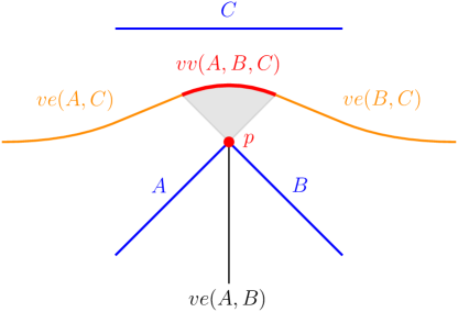
Figure 1: Degenerate case: $vv(A,B,C)$ consist of a whole arc and $ve(A,B)$ contains a region. Figure is best viewed in color.

If $A,B$ and $C$ are line segments and $A$ and $B$ intersect in a point $p$, it can happen that there are Voronoi vertices in $vv(A,B,C)$ for which the closest point in $A$ and $B$ is $p$. This may result in degenerate cases where a whole arc of the Voronoi diagram consists of Voronoi vertices and a region is part of a Voronoi edge (see Figure 1). For our distance queries, we are only interested in extreme points of the distance to the sites. These are Voronoi vertices that are not degenerate. We define the relevant Voronoi vertices as the Voronoi vertices for which the distance of the vertices to the sites is realizes by at least three distinct points, i.e.

$$rvv(A,B,C)=\left\{p\in vv(A,B,C)\ \middle|\begin{array}[]{l}\exists a,b,c\in A,B,C\text{ s.t. }a\neq b\neq c\neq a\text{ and }\\ d_{\overrightarrow{H}}(p,a)=d_{\overrightarrow{H}}(p,b)=d_{\overrightarrow{H}}(p,c)=d_{\overrightarrow{H}}(p,A\cup B\cup C)\end{array}\right\}$$

Additionally, we introduce the notion of Voronoi-vertex-candidates. Let $a=\overline{a_{1}a_{2}},b=\overline{b_{1}b_{2}}$ and $c=\overline{c_{1}c_{2}}$ be edges of a polygonal region that may contain holes. Consider their vertices and supporting lines $A=\{a_{1},a_{2},\ell(a)\}$, $B=\{b_{1},b_{2},\ell(b)\}$ and $C=\{c_{1},c_{2},\ell(c)\}$. Let $X\in A$, $Y\in B$ and $Z\in C$. If either $X,Y$ or $Z$ is a subset of one of the others, we set $V_{0}(X,Y,Z)=\emptyset$ otherwise let

$$V_{0}(X,Y,Z)=\{v\in{\mathbb{R}}^{2}\;|\;d_{\overrightarrow{H}}(v,X)=d_{\overrightarrow{H}}(v,Y)=d_{\overrightarrow{H}}(v,Z)\}$$

be the set of points with same distance to all sets $X,Y$ and $Z$. The set of Voronoi-vertex-candidates $V(a,b,c)$ of the line segments $a,b$ and $c$ is defined as the union over all points that have the same distance to fixed elements of $A$, $B$ and $C$, i.e.

$$V(a,b,c)=\bigcup_{X\in A,Y\in B,Z\in C}V_{0}(X,Y,Z).$$

Note that the Voronoi-vertex-candidates $V(a,b,c)$ contain all relevant Voronoi vertices $rvv(a,b,c)$ because a relevant Voronoi vertex $v$ has the same distance to all three edges and for each edge the distance to $v$ is either realized at one of the endpoints of the edge or at the orthogonal projection of $v$ to the supporting line of the edge.

4.3.2 Additional predicates

Let $P$ and $Q$ be two polygonal regions that may contain holes. Let further $\Delta\in{\mathbb{R}}_{+}$. In this section, we give predicates such that the Hausdorff distance query $d_{H}(P,Q)\leq\Delta$ is determined by them. The query depends on the two queries for the directed Hausdorff distances $d_{\overrightarrow{H}}(P,Q)\leq\Delta$ and $d_{\overrightarrow{H}}(Q,P)\leq\Delta$. We show, how to determine $d_{\overrightarrow{H}}(P,Q)\leq\Delta$, the other direction is analogous. The distance $d_{\overrightarrow{H}}(p,Q)$ for points $p\in P$ can be maximized at points in the interior of $P$ or at points at the boundary of $P$ (see Figure 2 for the two cases). Since these cases are different to analyze, we split the query into two general predicates.

• $({\mathcal{B}})$ (Boundary): This predicate returns true if and only if $d_{\overrightarrow{H}}(\partial P,Q)\leq\Delta$.

• $({\mathcal{I}})$ (Interior): This predicate returns true, if $d_{\overrightarrow{H}}(P,Q)\leq\Delta$. This predicate returns false if $d_{\overrightarrow{H}}(P,Q)>d_{\overrightarrow{H}}(\partial P,Q)$ and $d_{\overrightarrow{H}}(P,Q)>\Delta$.

Note that it is not defined what $({\mathcal{I}})$ returns if $d_{\overrightarrow{H}}(P,Q)=d_{\overrightarrow{H}}(\partial P,Q)$ and $d_{\overrightarrow{H}}(P,Q)>\Delta$. This does not matter, since the correctness of $d_{\overrightarrow{H}}(P,Q)\leq\Delta$ is still equivalent to both $({\mathcal{B}})$ and $({\mathcal{I}})$ being true.

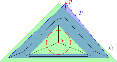
Figure 2: Illustration of the two cases: The point $p$ on the boundary of $P$ maximizes $d_{\overrightarrow{H}}(p,Q)$. The point $q$ in the interior of $Q$ that is a Voronoi vertex of the edges of $P$ maximizes $d_{\overrightarrow{H}}(q,P)$. Figure is best viewed in color.

Since $({\mathcal{B}})$ and $({\mathcal{I}})$ are very general, we define more detailed predicates that can be used to determine feasible truth values of $({\mathcal{B}})$ and $({\mathcal{I}})$. To determine $({\mathcal{B}})$, we need the following predicates in combination with ${\mathcal{P}}_{\ref{hpc2}}$ and ${\mathcal{P}}_{\ref{hpc4}}$ defined in Section 4.2:

• ($\mathcal{P}_{9}$): Given a vertex $p$ of $P$, this predicate returns true if and only if $p\in Q$.

• ($\mathcal{P}_{10}$): Given an edge $e_{1}$ of $P$ and an edge $e_{2}$ of $Q$, this predicate is equal to $e_{1}\cap e_{2}\neq\emptyset$.

• ($\mathcal{P}_{11}$): Given an directed edge $e_{1}$ of $P$ and two edges $e_{2}$ and $e_{3}$ of $Q$, this predicate is true if and only if $e_{1}\cap e_{2}\neq\emptyset$, $e_{1}\cap e_{3}\neq\emptyset$ and $e_{1}$ intersects $e_{2}$ before or at the same point that it intersects $e_{3}$.

• ($\mathcal{P}_{12}$): Given an directed edge $e_{1}$ of $P$ and two edges $e_{2}$ and $e_{3}$ of $Q$, this predicate is true if and only if $e_{1}\cap e_{2}\neq\emptyset$ and if there exists a point $b$ on $e_{3}$ such that $\lVert a-b\rVert\leq\Delta$ where $a$ is the first intersection point of $e_{1}\cap e_{2}$.

• ($\mathcal{P}_{13}$): Given an directed edge $e_{1}$ of $P$ and two edges $e_{2}$ and $e_{3}$ of $Q$, this predicate is true if and only if $e_{1}\cap e_{2}\neq\emptyset$ and if there exists a point $b$ on $e_{3}$ such that $\lVert a-b\rVert\leq\Delta$ where $a$ is the last intersection point of $e_{1}\cap e_{2}$.

Using Voronoi-vertex-candidates, we define the detailed predicates for determining $({\mathcal{I}})$:

• ($\mathcal{P}_{14}$): Given $4$ edges $e_{1},e_{2},e_{3},e_{4}$ of $Q$ and a point $v$ from the set of Voronoi-vertex-candidates $V(e_{1},e_{2},e_{3})$, this predicate returns true if and only if there exists a point $p\in e_{4}$, such that $\|v-p\|\leq\Delta$.

• ($\mathcal{P}_{15}$): Given $3$ edges $e_{1},e_{2},e_{3}$ of $Q$ and a point $v$ from the set of Voronoi-vertex-candidates $V(e_{1},e_{2},e_{3})$, this predicate returns true if and only if $v\in Q$.

• ($\mathcal{P}_{16}$): Given $3$ edges $e_{1},e_{2},e_{3}$ of $Q$ and a point $v$ from the set of Voronoi-vertex-candidates $V(e_{1},e_{2},e_{3})$, this predicate returns true if and only if $v\in P$.

Examples for the predicates ${\mathcal{P}}_{\ref{hprb1}},\dots\mathcal{P}_{\ref{hpri3}}$ are depicted in Figure 3.

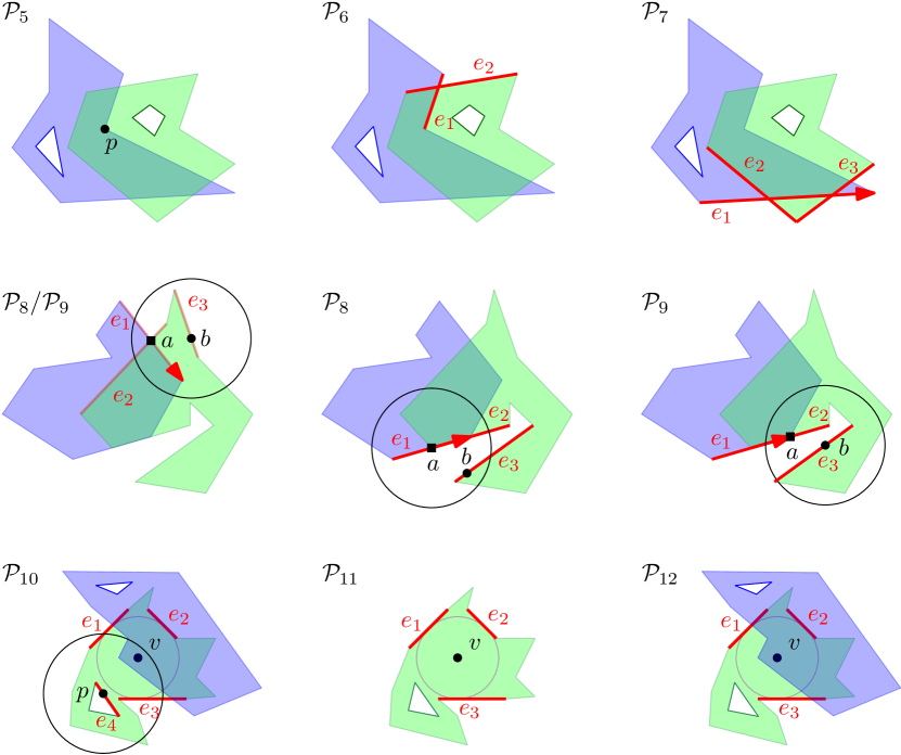
Figure 3: Illustration of the predicates ${\mathcal{P}}_{\ref{hprb1}},\dots,{\mathcal{P}}_{\ref{hpri3}}$ : In all depicted cases the corresponding predicates are true. Figure is best viewed in color.

Lemma 4.6.

For any two polygonal regions $P,Q$ that may contain holes, given the truth values of all predicates of the type ${\mathcal{P}}_{\ref{hpc2}},{\mathcal{P}}_{\ref{hpc4}},{\mathcal{P}}_{\ref{hprb1}},{\mathcal{P}}_{\ref{hprb2}},{\mathcal{P}}_{\ref{hprb3}},{\mathcal{P}}_{\ref{hprb4}}$ and ${\mathcal{P}}_{\ref{hprb5}}$ one can determine a feasible truth value for a predicate of type $({\mathcal{B}})$.

Proof 4.7.

To determine $({\mathcal{B}})$ it suffices to check for each edge $e$ of $P$ if $d_{\overrightarrow{H}}(e,Q)\leq\Delta$. If this is true for all edges, we return true, otherwise false. Let $e=\overline{uv}$ be an edge of $P$. We first determine which points of $e$ lie outside of $Q$. The ${\mathcal{P}}_{\ref{hprb1}}$ for the point $u$, tells us if $u$ lies in $Q$. Checking ${\mathcal{P}}_{\ref{hprb2}}$ and ${\mathcal{P}}_{\ref{hprb3}}$ for $e$ and all edges (respectively pairs of edges) of $Q$ then determines which edges of $Q$ get intersected and in which order they get intersected. Each intersection changes the state of the edge $e$ between lying inside and outside of $Q$. So in total we get a sequence of intersections of edges with $Q$ where we know for each part between two consecutive intersections, if this part is inside or outside of $Q$.

Let one subset $s=\overline{s_{1}s_{2}}$ of $e$ be given that is defined by two edges $e_{1}$ and $e_{2}$ of $Q$ that intersect $e$ consecutively. If $s$ lies inside of $Q$ then we have $d_{\overrightarrow{H}}(s,Q)=0$. If $s$ lies outside of $Q$ then we claim that $d_{\overrightarrow{H}}(s,Q)\leq\Delta$ if and only if there exists a sequence of edges $\overline{q_{j_{1}}q_{j_{1}+1}},\overline{q_{j_{2}}q_{j_{2}+1}},\dots,\overline{q_{j_{t}}q_{j_{t}+1}}$ for some integer value $t$, such that ${\mathcal{P}}_{\ref{hprb5}}(e,e_{1},\overline{q_{j_{1}}q_{j_{1}+1}})$ and ${\mathcal{P}}_{\ref{hprb4}}(e,e_{2},\overline{q_{j_{t}}q_{j_{t}+1}})$ evaluate to true and the conjugate

$$\bigwedge\limits_{i=1}^{t-1}{\mathcal{P}}_{\ref{hpc4}}(e,\overline{q_{j_{i}}q_{j_{i}+1}},\overline{q_{j_{i+1}}q_{j_{i+1}+1}})$$

evaluates to true. The proof of this claim is analogous to the key part of the proof of Lemma 7.1 in [9]. We include a full proof of the claim here for the sake of completeness.

Assume such a sequence $\overline{q_{j_{1}}q_{j_{1}+1}},\dots,\overline{q_{j_{t}}q_{j_{t}+1}}$ exists. In this case, there exists a sequence of points $a_{1},\dots,a_{t}$ on the line supporting $s$, with $a_{1}=s_{1}$, $a_{t}=s_{2}$, and such that for $1\leq i<t$, $a_{i},a_{i+1}\in D_{\Delta}(\overline{q_{j_{i}}q_{j_{i}+1}})$. That is, two consecutive points of the sequence are contained in the same stadium. Indeed, for $i=1$, we have that there exists points $a_{1},a_{2}$ with the needed properties since the predicates ${\mathcal{P}}_{\ref{hprb5}}(e,e_{1},\overline{q_{j_{1}}q_{j_{1}+1}})$ and ${\mathcal{P}}_{\ref{hpc4}}(e,\overline{q_{j_{1}}q_{j_{1}+1}},\overline{q_{j_{2}}q_{j_{2}+1}})$ evaluate to true. Likewise, for $i=t-1$, it is implied by the corresponding ${\mathcal{P}}_{\ref{hprb4}}$ and ${\mathcal{P}}_{\ref{hpc4}}$ predicates and for the remaining $1<i<t-1$ it follows from the corresponding ${\mathcal{P}}_{\ref{hpc4}}$ predicates. Now, since each stadium is a convex set, it follows that each line segment connecting two consecutive points of this sequence $a_{i},a_{i+1}$ is contained in one of the stadiums.Note that the set of line segments obtained this way forms a connected polygonal curve which fully covers the line segment $s$. It follows that

$$s\subseteq\bigcup_{0\leq i<t}\overline{a_{i}a_{i+1}}\subseteq\bigcup_{0\leq i<t}D_{\Delta}(\overline{q_{j_{i}}q_{j_{i}+1}})$$

Therefore, any point on $s$ is within distance $\Delta$ of some point on $Q$ and thus $d_{\overrightarrow{H}}(s,Q)\leq\Delta$

For the other direction of the proof, assume that $d_{\overrightarrow{H}}(s,Q)\leq\Delta$. Let $E(Q)$ be the set of all edges of $Q$ The definition of the directed Hausdorff distance implies that

$$s\subseteq\bigcup_{e\in E(Q)}D_{\Delta}(e)$$

since any point on the line segment $s$ must be within distance $\Delta$ of some point on the curve $Q$. Consider the intersections of the line segment $s$ with the boundaries of stadiums

$$s\cap\bigcup_{e\in E(Q)}\partial D_{\Delta}(e).$$

Let $w$ be the number of intersection points and let $l=w+2$. We claim that this implies that there exists a sequence of edges $\overline{q_{j_{1}}q_{j_{1}+1}},\overline{q_{j_{2}}q_{j_{2}+1}},\dots,\overline{q_{j_{t}}q_{j_{t}+1}}$ with the properties stated above. let $a_{1}=s_{2}$, $a_{t}=s_{2}$ and let $a_{i}$ for $1<i<t$ be the intersection points ordered in the direction of the line segment $s$. By construction, it must be that each $a_{i}$ for $1<i<t$ is contained in the intersection of two stadiums, since it is the intersection with the boundary of a stadium and the entire edge is covered by the union of stadiums. Moreover, two consecutive points $a_{i},a_{i+1}$ are contained in exactly the same subset of stadiums - otherwise there would be another intersection point with boundary of a stadium in between $a_{i}$ and $a_{i+1}$. This implies a set of true predicates of type ${\mathcal{P}}_{\ref{hpc4}}$ with the properties defined above. The predicates of type ${\mathcal{P}}_{\ref{hprb4}}$ and ${\mathcal{P}}_{\ref{hprb5}}$ follow trivially from the definitions of $s_{1}$, $s_{2}$ and the directed Hausdorff distance. This concludes the proof of the other direction.

It remains to consider the first and last parts of $e$. Let $s$ be a subset of $e$ defined by its boundaries $s_{1},s_{2}$ where one of the boundaries is one of the vertices $u$ and $v$ of $e$ and the other boundary is the closest intersection of $e$ with an edge of $Q$ or (if this does not exist) the other vertex of $e$. The proof for this case is analogous to the previous case. It only needs predicates of type ${\mathcal{P}}_{\ref{hpc2}}$ for $u$ and $v$ instead of the respective predicates of type ${\mathcal{P}}_{\ref{hprb5}}$ and ${\mathcal{P}}_{\ref{hprb4}}$.

Lemma 4.8.

For any two polygonal regions $P,Q$, given the truth values of all predicates of the type ${\mathcal{P}}_{\ref{hpri1}},{\mathcal{P}}_{\ref{hpri2}}$ and ${\mathcal{P}}_{\ref{hpri3}}$ one can determine a feasible truth value for a predicate of type $({\mathcal{I}})$.

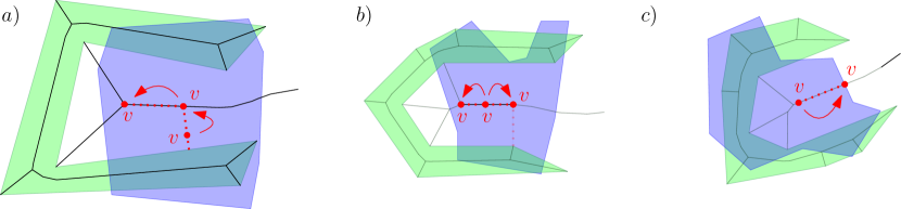
Figure 4: Illustration of the different cases in the proof of Lemma 4.8. It is demonstrated how $v$ can be moved to either increase the distance to $Q$ (a) or to stay in the same distance to $Q$ (b,c). Figure is best viewed in color.

Proof 4.9.

We claim that, if $d_{\overrightarrow{H}}(P,Q)>d_{\overrightarrow{H}}(\partial P,Q)$ and $d_{\overrightarrow{H}}(P,Q)>\Delta$ then there has to be a point $v$ in the interior of $P$ that maximizes the Hausdorff distance to $Q$ (i.e. $d_{\overrightarrow{H}}(v,Q)=\max_{p\in P}(d_{\overrightarrow{H}}(p,Q))$) and that is a relevant Voronoi vertex of the edges of $Q$. Before we prove the claim, we show that it implies the statement of the lemma. It follows from the claim that in case of $d_{\overrightarrow{H}}(P,Q)>d_{\overrightarrow{H}}(\partial P,Q)$ and $d_{\overrightarrow{H}}(P,Q)>\Delta$ there is a relevant Voronoi vertex $v$ that lies in $P$ and outside of $Q$ with $d_{\overrightarrow{H}}(v,e)>\Delta$ for all edges $e$ of $Q$. The predicates ${\mathcal{P}}_{\ref{hpri1}},{\mathcal{P}}_{\ref{hpri2}}$ and ${\mathcal{P}}_{\ref{hpri3}}$ check exactly these properties for a superset of the relevant Voronoi vertices of the edges $Q$. So, we set $({\mathcal{I}})$ to false, if and only if there is a vertex in this superset that fulfills ${\mathcal{P}}_{\ref{hpri3}}$, does not fulfill ${\mathcal{P}}_{\ref{hpri2}}$ and does not fulfill ${\mathcal{P}}_{\ref{hpri1}}$ for any edge of $Q$. Since all relevant Voronoi vertices are checked, $({\mathcal{I}})$ will be set to false in all relevant cases. On the other hand, if we have $d_{\overrightarrow{H}}(P,Q)\leq\Delta$ then there will be no point that is in $P$, outside of $Q$ and has distance greater $\Delta$ to all edges of $Q$ and $({\mathcal{I}})$ is set to true. It remains to show the claim.

We prove the claim by contradiction. We assume that $d_{\overrightarrow{H}}(P,Q)>\Delta$ and $d_{\overrightarrow{H}}(P,Q)>d_{\overrightarrow{H}}(\partial P,Q)$ and that none of the points in the interior of $P$ that maximize the Hausdorff distance to $Q$ is a relevant Voronoi vertex of the edges of $Q$. Let $v\in P$ be a point maximizing $d_{\overrightarrow{H}}(v,Q)$. Assume that $v$ lies in the Voronoi region of an edge $e$ of $Q$. Then $d_{\overrightarrow{H}}(v,Q)$ can be increased by moving $v$ in perpendicular direction away from $e$ (see Fig. 4a)). This would contradict that $v$ maximizies $d_{\overrightarrow{H}}(v,Q)$. So instead, assume that $v$ lies on the Voronoi edge defined by the Voronoi regions of two edges $e_{1}$ and $e_{2}$ of $Q$ and that $v$ is not a relevant Voronoi vertex. If $e_{1}$ and $e_{2}$ are not parallel, then it can be shown with a straight forward case analysis that there is a direction in which $v$ can be moved along the Voronoi diagram to increase $d_{\overrightarrow{H}}(v,Q)$ (see Fig. 4a)). The direction depends on the the closest points $v_{1},v_{2}$ to $v$ on $e_{1},e_{2}$. If $v_{2}1$ and $v_{2}$ are perpendicular projections of $v$ to $e_{1}$ and $e_{2}$ then $v$ can be moved along the angle bisector of $e_{1}$ and $e_{2}$ away from the intersection of $\ell(e_{1})$ and $\ell(e_{2})$. If only one of $v_{1}$ and $v_{2}$ is not a perpendicular projection then $v$ can be moved along the parabola defined by $v_{1}$ and $e_{2}$ (or $v_{2}$ and $e_{1}$) in both directions. If both $v_{1}$ and $v_{2}$ are not a perpendicular projection then $v$ can be moved in any direction $d$ with $\langle v-v_{2},d\rangle\geq 0$ and $\langle v-v_{1},d\rangle\geq 0$. If $e_{1}$ and $e_{2}$ are parallel, it can happen that locally $d_{\overrightarrow{H}}(p,Q)$ stays constant for moving $v$ along the Voronoi edge in both directions until either a relevant Voronoi vertex is reached (see Fig. 4b)), the boundary of $P$ is reached (see Fig. 4c)) or the orthogonal projection of $v$ to either one of the edges $e_{1}$ and $e_{2}$ reaches an endpoint of the respective edge (see Fig. 4b)). In all three cases, we get a contradiction. The first case contradicts the assumption that there is no relevant Voronoi vertex $v$ that maximizes $d_{\overrightarrow{H}}(v,Q)$, the second case contradicts the assumption that $d_{\overrightarrow{H}}(P,Q)>d_{\overrightarrow{H}}(\partial P,Q)$ and in the third case $d_{\overrightarrow{H}}(p,Q)$ would start increasing and contradict that $v$ maximizes $d_{\overrightarrow{H}}(v,Q)$.

5 The predicates are simple

It remains to show that the predicates defined in Section 4.2 and 4.3 can be determined by a polynomial number of simple predicates. Corollary 4.2 then implies that all considered range spaces have $VCdim({\mathcal{R}}_{\rho,k})$ in $O(dk\log(km))$.

5.1 Technical lemmas

In this section, we establish some general lemmas that will help us to show that predicates can be determined by a polynomial number of simple predicates. We first introduce some new notation.

Definition 5.1.

Let $d\in{\mathbb{N}}$. We call a function $f:{\mathbb{R}}^{d}\rightarrow{\mathbb{R}}$ well behaved if $f$ is a linear combination of constantly many rational functions of constant degree. Let $x_{1}\in{\mathbb{R}}^{d_{1}},\dots x_{i}\in{\mathbb{R}}^{d_{i}}$ with $\sum_{j=1}^{i}d_{j}=d$. Let $X=\{x_{1},\dots x_{i}\}$ and $x$ be the concatenation of $x_{1},\dots,x_{i}$. We denote $f(x)$ also with $f(x_{1},\dots,x_{i})$ or $f(X)$.

For many of our predicates, we have to determine the order of two points on a line. For example, when we check if the intersections of a line with other geometric objects overlap. The following lemma shows, that determining the order is simple.

Lemma 5.2.

Let $d\in{\mathbb{N}}$. Let $P\subset{\mathbb{R}}^{d}$ be a finite set of points and $p,q\in P$. Consider two points $v$ and $w$ on the line $\ell(\overline{pq})$ given by

$$v =p+t_{1}(P)(q-p)$$

$$w =p+t_{2}(P)(q-p)$$

with $t_{i}(P)=a_{i}(P)+b_{i}(P)\sqrt{c_{i}(P)}$ where $a_{i},b_{i}$ and $c_{i}$ are well behaved functions for $i\in\{1,2\}$. It is a simple predicate to determine the order of $v$ and $w$ in direction $(q-p)$.

Note that the order in Lemma 5.2 can be decided by solving $t_{1}(P)\geq t_{2}(P)$. So Lemma 5.2 directly follows from the following more general lemma.

Lemma 5.3.

Consider the 3 inequalities

$$a(x) \geq 0$$ (1)

$$b\left(x,\sqrt{c(x)},\sqrt{d(x)}\right) \geq 0$$ (2)

$$e\left(x,\sqrt{f(x)},\sqrt{g\left(x,\sqrt{f(x)}\right)}\right) \geq 0$$ (3)

for well behaved functions $a,b,c,d,e,f,g$. The following statements hold:

1. Inequality (1) is simple.

2. Inequality (2) is simple if $c(x)\geq 0$ and $d(x)\geq 0$.

3. Inequality (3) is simple if $f(x)\geq 0$ and $g(x,\sqrt{f(x)})\geq 0$.

Observe that the inequalities $c(x)\geq 0$, $d(x)\geq 0$ and $f(x)\geq 0$ are simple by the first statement and $g(x,\sqrt{f(x)})\geq 0$ is simple by the second statement.

Proof 5.4 (Proof of Lemma 5.3).

1. If we multiply both sides of the inequality $a(x)\geq 0$ by the square of the product of all denominators of the rational functions in $a$, then we get an equivalent inequality that only consists of a polynomial of constant degree on the left side and $0$ on the right side. This inequality is by definition simple.

2. If we also here multiply both sides of the inequality $b\left(x,\sqrt{c(x)},\sqrt{d(x)}\right)\geq 0$ by the square of the product of all denominators of the rational functions in $b$, then we get an equivalent inequality

$$b_{0}\left(x,\sqrt{c(x)},\sqrt{d(x)}\right)\geq 0$$

where $b_{0}$ is a polynomial of constant degree. If we rearrange the terms in $b_{0}$ we get an equivalent inequality

$$b_{1}(x)+b_{2}(x)\sqrt{c(x)}\sqrt{d(x)}\leq b_{3}(x)\sqrt{c(x)}+b_{4}(x)\sqrt{d(x)}$$ (4)

where $b_{1},b_{2},b_{3}$ and $b_{4}$ are polynomials of constant degree. To show that (4) is simple, we first show that the sign value of both sides of $(4)$ are determined by a simple inequality. To check the sign of the left side

$$b_{1}(x)+b_{2}(x)\sqrt{c(x)}\sqrt{d(x)}\geq 0$$ (5)

we have to check the signs of $b_{1}(x)$ and $b_{2}(x)$. Since $b_{1}$ and $b_{2}$ are polynomials of constant degree, their signs are determined by a simple inequality. If $sgn(b_{0}(x))=sgn(b_{1}(x))$ then the truth value of (5) is directly implied. Otherwise, we can square both sides of

$$b_{2}(x)\sqrt{c(x)}\sqrt{d(x)}\geq-b_{1}(x)$$

and (5) is equivalent to

$$b_{2}(x)^{2}c(x)d(x)\geq b_{1}(x)^{2}.$$

After rearranging, this is a simple inequality because it has the same form as (1). The check for the sign value of the right side of (4) is analogous. If the sign values of the two sides differ, we get an immediate solution for the truth value of (4). Otherwise we square both sides and (4) is equivalent to

$$b_{1}(x)^{2}+b_{2}(x)^{2}c(x)d(x)+2b_{1}(x)b_{2}(x)\sqrt{c(x)}\sqrt{d(x)} \leq$$

$$b_{3}(x)^{2}c(x)+b_{4}(x)^{2}d(x)+2b_{3}(x)b_{4}(x)\sqrt{c(x)}\sqrt{d(x)}$$ (6)

Multiplying both sides of (6) by the square of the product of all denominators of the rational functions in $c$ and $d$ and then rearranging the terms gives and equivalent inequality

$$b_{5}(x)+b_{6}(x)\sqrt{c(x)}\sqrt{d(x)}\geq 0.$$

where $b_{5}$ and $b_{6}$ are polynomials of constant degree. This inequality is simple as it has the same form as (5). In total, inequality (2) is simple as a constant combination of simple predicates.

3. The structure of the proof of the third statement is very similar to the structure of the proof of the second statement. We still include the details here for completeness.

If we multiply both sides of inequality $e\left(x,\sqrt{f(x)},\sqrt{g\left(x,\sqrt{f(x)}\right)}\right)\geq 0$ by the square of the product of all denominators of the rational functions in $a$ and rearrange some terms, then we get an equivalent inequality

$$e_{1}(x)+e_{2}(x)\sqrt{f(x)}\leq e_{3}(x)\sqrt{g\left(x,\sqrt{f(x)}\right)}+e_{4}(x)\sqrt{f(x)}\sqrt{g\left(x,\sqrt{f(x)}\right)}$$ (7)

where $e_{1},e_{2},e_{3}$ and $e_{4}$ are polynomials of constant degree. We again show that the sign values of both sides of (7) are determined by a simple inequality. The check of the left side is analogous to checking inequality (5). To check the right side

$$e_{3}(x)\sqrt{g\left(x,\sqrt{f(x)}\right)}+e_{4}(x)\sqrt{f(x)}\sqrt{g\left(x,\sqrt{f(x)}\right)}\geq 0$$ (8)

we have to check the signs of $e_{3}(x)$ and $e_{4}(x)$. Since $e_{3}$ and $e_{4}$ are polynomials of constant degree, their signs are determined by a simple inequality. If $sgn(e_{3}(x))=sgn(e_{4}(x))$ then the truth value of (5) is directly implied. Otherwise, we can square both sides of

$$-e_{3}(x)\sqrt{g\left(x,\sqrt{f(x)}\right)}\leq e_{4}(x)\sqrt{f(x)}\sqrt{g\left(x,\sqrt{f(x)}\right)}$$

to get that (8) is equivalent to

$$e_{3}(x)^{2}g\left(x,\sqrt{f(x)}\right)\leq e_{4}(x)^{2}f(x)g\left(x,\sqrt{f(x)}\right).$$ (9)

After rearranging, this is a simple inequality because it has the same form as (2). If the sign values of the two sides of inequality (3) differ, we get an immediate solution for it. Otherwise we get the following equivalent inequality by squaring both sides:

$$e_{1}(x)^{2}+e_{2}(x)^{2}f(x)+2e_{1}(x)e_{2}(x)\sqrt{f(x)} \leq$$

$$e_{3}(x)^{2}g\left(x,\sqrt{f(x)}\right)+e_{4}(x)^{2}g\left(x,\sqrt{f(x)}\right)+e_{3}(x)e_{4}(x)\sqrt{f(x)}g\left(x,\sqrt{f(x)}\right)$$ . (10)

Rearranging the terms in (10) gives an inequality

$$e_{0}(x,\sqrt{f(x)})\geq 0$$

where $e_{0}$ is a well behaved function. Since this inequality is a special case of inequality (2) it is simple.

In general, we have to deal with different types of points as part of the predicates. We classify them in the following way.

Definition 5.5.

Let $d\in{\mathbb{N}}$ and $\Delta\in{\mathbb{R}}_{+}$. Let $P\subset{\mathbb{R}}^{d}$ be a finite set of points and $p,q\in P$. Let further $v\in{\mathbb{R}}^{d}$. We say that $v$ is a point of root-type 1, 2 or 3 with respect to $P$ if and only if the coordinates of $v=(v_{1},\dots,v_{d})$ can be written as

1. $v_{i}=a_{i}(P)$

2. $v_{i}=b_{i}\left(P,\sqrt{c(P)},\sqrt{d(P)}\right)$

3. $v_{i}=e_{i}\left(P,\sqrt{f(P)},\sqrt{g\left(P,\sqrt{f(P)}\right)}\right)$

where $a_{i},b_{i},c,d,e_{i},f,g$ are well behaved functions for all $i$ with $c(P)\geq 0$, $d(P)\geq 0$, $f(P)\geq 0$ and $g\left(P,\sqrt{f(P)}\right)\geq 0$.

Lemma 5.6.

Let $a=\overline{a_{1}a_{2}},b=\overline{b_{1}b_{2}}$ and $c=\overline{c_{1}c_{2}}$ be edges of a polygonal region that may contain holes. Let $P=\{a_{1},a_{2},b_{1},b_{2},c_{1},c_{2}\}$. All points in the set of Voronoi-vertex-candidates $V(a,b,c)$ are of root-type 1, 2 or 3 with respect to $P$. There is only a constant number of combinations of well behaved functions that can define a point in $V(a,b,c)$ (by using these function as the well behaved functions in Definition 5.5). These combinations are uniquely determined by $a,b$ and $c$. For each combination, it is a simple predicate to check if it defines a point in $V(a,b,c)$.

Proof 5.7.

Consider the sets $A=\{a_{1},a_{2},\ell(a)\}$, $B=\{b_{1},b_{2},\ell(b)\}$ and $C=\{c_{1},c_{2},\ell(c)\}$. Let $X\in A$, $Y\in B$ and $Z\in C$. This combination of $X,Y$ and $Z$ only contributes points to $V(a,b,c)$ if neither of $X,Y$ and $Z$ is a subset of one of the others. This can be checked with a simple predicate by Lemma 5.3: To check if two points $(u_{1},u_{2})$ and $(v_{1},v_{2})$ are the same, we need to check if $u_{1}=v_{1}$ and $u_{2}=v_{2}$. Checking an equation $(=)$ can be done by checking both inequalities $(\leq)$ and $(\geq)$. Checking if a point $(u_{1},u_{2})$ lies on a line $\ell(\overline{vw})$ with $v=(v_{1},v_{2})$ and $w=(w_{1},w_{2})$ can be done by checking if there exists a $t$ such that

$$\begin{pmatrix}v_{1}\\ v_{2}\end{pmatrix}+t\begin{pmatrix}w_{1}-v_{1}\\ w_{2}-v_{2}\end{pmatrix}=\begin{pmatrix}u_{1}\\ u_{2}\end{pmatrix}.$$

This is equivalent to the following equation being true.

$$v_{2}+\frac{u_{1}-v_{1}}{w_{1}-v_{1}}(w_{2}-v_{2})=u_{2}$$

To check if two lines $\ell(\overline{pq})$ and $\ell(\overline{vw})$ coincide, we have to check if $p$ is on the line $\ell(\overline{vw})$ as before and additionally if the lines have the same slope. This can be done by checking the truth value of $\frac{p_{2}-q_{2}}{p_{1}-q_{1}}=\frac{v_{2}-w_{2}}{v_{1}-w_{1}}$.

If the checks determine that one of $X,Y$ and $Z$ is the subset of one of the others, then all combinations of well behaved functions based on the combination $X,Y,Z$ can be ignored. Otherwise, we have 4 different cases for the types of objects $X,Y,Z$. It can be that there are 3 points, 2 points and 1 line, 1 point and 2 lines or 3 lines. Consider the biscetors of the pairs $(X,Y)$, $(X,Z)$ and $(Y,Z)$. The Voronoi-vertex-candidates are the intersections of these bisectors. It suffices to find the intersections of two bisectors, since the third one intersects the other two in the same points (by definition).

Case 1 (3 points): The bisector of the 3 points $u=(u_{1},u_{2})$, $v=(v_{1},v_{2})$ and $w=(w_{1},w_{2})$ intersect if the points are not colinear. This is just a simple predicate to check, as we have seen before by checking if $u$ lies on the line $\ell(\overline{vw})$. Assume $u$, $v$ and $w$ are not colinear. Then the bisector of $u$ and $v$ parameterized in $s$ is given by

$$\ell_{1}(s)=\frac{1}{2}\begin{pmatrix}u_{1}+v_{1}\\ u_{2}+v_{2}\end{pmatrix}+s\begin{pmatrix}v_{2}-u_{2}\\ u_{1}-v_{1}\end{pmatrix}$$

and the bisector of $w$ and $v$ parameterized in $t$ is given by

$$\ell_{2}(s)=\frac{1}{2}\begin{pmatrix}w_{1}+v_{1}\\ w_{2}+v_{2}\end{pmatrix}+t\begin{pmatrix}v_{2}-w_{2}\\ w_{1}-v_{1}\end{pmatrix}.$$

So if we set $\ell_{1}(s)=\ell_{2}(t)$, we get two linear equations with the two variable $s$ and $t$ of the form

$$f(P)+g(P)s+h(P)t=0$$

where $f,g,h$ are well behaved functions. Since the points where not colinear, the solution for $t$ is a uniquely determined well behaved function and therefore the intersection point of the bisectors is a point of root-type 1.

Case 2 (2 points, 1 line): Note that a line between two points in $P$ can be written as

$$f_{1}(P)x+f_{2}(P)y+f_{3}(P)=0$$

where $f_{1},f_{2},f_{3}$ are well behaved functions. The bisector between such a line and a point $(u_{1},u_{2})$ is given by the parabola

$$\frac{f_{1}(P)x+f_{2}(P)y+f_{3}(P)}{f_{1}(P)^{2}+f_{2}(P)^{2}}=(x-u_{1})^{2}+(y-u_{2})^{2}.$$ (11)

For the bisector of two points $u=(u_{1},u_{2})$ and $(v_{1},v_{2})$ parameterized in $t$, we have as before

$$x =\frac{1}{2}(u_{1}+v_{1})+t(v_{2}-u_{2})$$ (12)

$$y =\frac{1}{2}(u_{2}+v_{2})+t(u_{1}-v_{1})$$ (13)

Inserting (12) and (13) into (11) gives a quadratic equation in $t$ with solutions of the form

$$t_{1/2}=g_{1}(P)\pm\sqrt{g_{2}(P)}$$

where $g_{1},g_{2}$ are well behaved functions. If $g_{2}(P)<0$ then there is no intersection. This can be checked with a simple predicate by Lemma 5.3. Otherwise the (up to two) intersections of the two bisectors are points of root-type 2.

Case 3 (1 point, 2 lines): In this case it can happen that the 2 lines are parallel. We have already shown that it can be checked by a simple predicate if the two lines have the same slope. Let the two lines be $\ell(\overline{pq})$ and $\ell(\overline{vw})$ with $p=(p_{1},p_{2})$, $q=(q_{1},q_{2})$, $v=(v_{1},v_{2})$ and $w=(w_{1},w_{2})$.

Case 3.1 (2 lines are parallel): The bisector of $\ell(\overline{pq})$ and $\ell(\overline{vw})$ parameterized in $t$ is given by

$$x =\frac{1}{2}(p_{1}+v_{1})+t(p_{1}-q_{1})$$

$$y =\frac{1}{2}(p_{2}+v_{2})+t(p_{2}-q_{2})$$

So analogous to Case 2, the existence of an intersection of such a bisector with a parabola of the form (11) is a simple predicate and if an intersection exists, the (up tp two) intersections are points of root-type 2.

Case 3.2 (2 lines are not parallel): The bisector of $\ell(\overline{pq})$ and $\ell(\overline{vw})$ is the union of their two angle bisectors. The angle bisectors are uniquely determined by the intersection point of $\ell(\overline{pq})$ and $\ell(\overline{vw})$ and their slopes. Analogous to Case 1, it can be seen that the intersection of $\ell(\overline{pq})$ and $\ell(\overline{vw})$ is a point $(g_{1}(P),g_{2}(P))$ where $g_{1}$ and $g_{2}$ are well behaved functions. Let $m^{\prime}$ and $m^{\prime\prime}$ be the slopes of $\ell(\overline{pq})$ and $\ell(\overline{vw})$. The angle of two lines with slope $m^{\prime}$ and $m^{\prime\prime}$ is given by $\tan^{-1}(\frac{m^{\prime}-m^{\prime\prime}}{1+m^{\prime}m^{\prime\prime}})$. Since the angle bisectors have the same angle to both of the lines just with different sign, we get for the slope $m$ of an angle bisector that

$$\frac{m-m^{\prime}}{1+mm^{\prime}}=-\frac{m-m^{\prime\prime}}{1+mm^{\prime\prime}}$$

Solving this equation for $m$ gives two solutions of the form

$$m_{1/2}=g_{3}(P)\pm\sqrt{g_{4}(P)}$$

where $g_{3}$ and $g_{4}$ are well behaved functions with $g_{4}(P)\geq 0$. So in total the angle bisectors are given by

$$x =g_{1}(P)+t$$ (14)

$$y =g_{2}(P)+t(g_{3}(P)\pm\sqrt{g_{4}(P)}$$ (15)

For each of the angle bisectors, inserting (14) and (15) in (11) gives a quadratic equation in $t$ of the form

$$t^{2}h_{1}(P,\sqrt{g_{4}(P)})+th_{2}(P,\sqrt{g_{4}(P)})+h_{3}(P,\sqrt{g_{4}(P)})$$

where $h_{1},h_{2},h_{3}$ are well behaved functions. The solutions for $t$ therefore have the form

$$t_{1/2}=h_{4}(P,\sqrt{g_{4}(P)})\pm\sqrt{h_{5}(P,\sqrt{g_{4}(P)})}$$

where $h_{4},h_{5}$ are well behaved functions. If $h_{5}(P,\sqrt{g_{4}(P)})<0$, then there is no intersection. This is simple by Lemma 5.3. Otherwise the (up to two) intersections are points of root-type 3. In total there can be up to four intersection because there are two angle bisectors.

Case 4 (3 lines): As we have seen before, all occuring bisectors are unions of (up to two) lines of the form given in (14) and (15). Note that the bisector of two parallel lines can also be realized in that way by setting $g_{4}(P)=0$. Consider the intersection of two of these bisectors $\ell_{1}(s)$ and $\ell_{2}(t)$ where

$$\ell_{1}(s)=\begin{pmatrix}f_{1}(P)\\ f_{2}(P)\end{pmatrix}+s\begin{pmatrix}1\\ f_{3}(P)+\sqrt{f_{4}(P)}\end{pmatrix}$$

and

$$\ell_{2}(t)=\begin{pmatrix}g_{1}(P)\\ g_{2}(P)\end{pmatrix}+t\begin{pmatrix}1\\ g_{3}(P)+\sqrt{g_{4}(P)}\end{pmatrix}$$

with $f_{1-4},g_{1-4}$ being well behaved functions, $f_{4}(P)\geq 0$ and $g_{4}(P)\geq 0$. If we set $\ell_{1}(s)=\ell_{2}(t)$, we get a system of two linear equations in $s$ and $t$. The system has a unique solution if $f_{3}(P)+\sqrt{f_{4}(P)}\neq g_{3}(P)+\sqrt{g_{4}(P)}$. Otherwise, there is no intersection (since the lines $X,Y,Z$ may not have the same slope). The Inequality is simple by Lemma 5.3. If there is a solution for $t$ it has the form

$$t=h(P,\sqrt{f_{4}(P)},\sqrt{g_{4}(P)})$$

where $h$ is a well behaved function. So the intersection is a point of root-type 2. The proof is analogous if one or two of the consider bisectors have a minus in (15).

A reoccurring predicate is the decision if a given point is within a given distance to a given edge. We show in the following lemma that such predicates are simple.

Lemma 5.8.

Let $d\in{\mathbb{N}}$ and $\Delta\in{\mathbb{R}}_{+}$. Let $P\subset{\mathbb{R}}^{d}$ be a finite set of points and $p,q\in P$. Let further $v\in{\mathbb{R}}^{d}$. Let ${\mathcal{P}}$ be the predicate to decide if there exists a point $u\in\overline{pq}$ such that $\lVert u-v\rVert\leq\Delta$. ${\mathcal{P}}$ is simple if $v$ is a point of root-type 1, 2 or 3 w.r.t. $P$.

Proof 5.9.

The truth value of the predicate ${\mathcal{P}}$ can be determined by checking if $v$ is in the stadium $D_{\Delta}(\overline{pq})$. For this check, it suffices to check if $v$ is in at least one of $B_{\Delta}(p)$, $B_{\Delta}(q)$ and $R_{\Delta}(\overline{pq})$. For $B_{\Delta}(p)$ and $B_{\Delta}(q)$ ,we have to check the inequalities

$$\Delta^{2}-\lVert v-p\rVert^{2} \geq 0$$ (16)

$$\Delta^{2}-\lVert v-q\rVert^{2} \geq 0.$$ (17)

To check if $v\in R_{\Delta}(\overline{pq})$ consider the closest point $s$ to $v$ on the line $\ell(\overline{pq})$. The truth value of

$$\Delta^{2}-\lVert s-v\rVert^{2}\geq 0$$ (18)

uniquely determines if $v$ is in the cylinder $C_{\Delta}(\overline{pq})$. The truth values of

$$\lVert p-q\rVert^{2}-\lVert p-s\rVert^{2} \geq 0,$$ (19)

$$\lVert p-q\rVert^{2}-\lVert q-s\rVert^{2} \geq 0$$ (20)

further determine if $s$ is on the edge $\overline{pq}$. So the truth values of the inequalities (18), (19) and (20) determine the truth value of $v\in R_{\Delta}(\overline{pq})$. The closest point to $v$ on the line $\ell(\overline{pq})$ is

$$s=p+\frac{(p-q)\langle(p-q),v\rangle}{\lVert p-q\rVert^{2}}.$$

For each coordinate of $s$, we have

$$s_{j}=p_{j}+(p_{j}-q_{j})\frac{\sum_{i=1}^{d}(p_{i}-q_{i})v_{i}}{\sum_{i=1}^{d}(p_{i}-q_{i})^{2}}.$$

Note that for any two points $x,y\in{\mathbb{R}}^{d}$, we have that

$$\lVert x-y\rVert^{2}=\sum_{i=1}^{d}(x_{i}-y_{i})^{2}$$

is a polynomial of constant degree. So for any of the inequalities (16), (17), (18), (19) and (20) the following is true. If we insert all coordinates of $v$ into the inequality and rearrange the terms, we get (depending on the root-type of $v$) an equivalent inequality of one of the following types

$$h_{1}(P) \geq 0$$

$$h_{2}\left(P,\sqrt{c(P)},\sqrt{d(P)}\right) \geq 0$$

$$h_{3}\left(P,\sqrt{f(P)},\sqrt{g\left(P,\sqrt{f(P)}\right)}\right) \geq 0$$

where $c,d,f,g,h_{1},h_{2}$ and $h_{3}$ are well behaved functions. By Lemma 5.3 all three types of inequalities are simple. So, in all three cases of different coordinates of $v$ only a constant number of simple inequalities have to be checked to determine ${\mathcal{P}}$. Therefore ${\mathcal{P}}$ is simple.

Many of our predicates depend on the intersections of geometric objects. We address in the next lemmas that these intersections have nice properties and that the existence of these intersections can be determined by a simple predicate.

Lemma 5.10.

Let $P\subset{\mathbb{R}}^{2}$ be a finite set of points and $p=(p_{1},p_{2}),q=(q_{1},q_{2})\in P$. Consider the intersection of the horizontal ray $hr(v)$ starting at $v\in{\mathbb{R}}^{2}$ and the edge $\overline{pq}$. Let ${\mathcal{P}}$ be the predicate to decide if $hr(v)\cap\overline{pq}\neq\emptyset$. ${\mathcal{P}}$ is simple if $v$ is a point of root-type 1, 2 or 3 w.r.t. $P$.

Proof 5.11.

To check if $hr(v)$ intersects the line $\ell(\overline{pq})$, one can first check if $p_{2}-q_{2}=0$ by checking the simple inequalities $p_{2}-q_{2}\geq 0$ and $p_{2}-q_{2}\leq 0$. If this is the case, then an intersection is still possible if $v_{2}-p_{2}=0$. The inequalities $v_{2}-p_{2}\geq 0$ and $v_{2}-p_{2}\leq 0$ are also simple by Lemma 5.3. The root-type of $v$ determines which case of the lemma to use. If $v_{2}-p_{2}\leq 0$ is also true, then it can be determined if $hr(v)\cap\overline{pq}\neq\emptyset$ by checking $v_{1}-p_{1}\geq 0$ and $v_{1}-q_{1}\geq 0$. These inequalities determine the relative positions of $v$ to $p$a and $q$ on the horizontal line. They are again simple by Lemma 5.3.

If $p_{2}\neq q_{2}$, then the intersection of the horizontal line through $v$ and the line $\ell(\overline{pq})$ is a uniquely defined point $s=p+t(p-q)$ with $t=\frac{(v_{2}-p_{2})}{(p_{2}-q_{2})}$. In this case it remains to check if $1\geq t$ and $t\geq 0$ to see if $s$ lies on the edge $\overline{pq}$ and to check if $s_{1}\geq v_{1}$ to see if $s$ lies on the right side of $v$ and is on the ray $hr(v)$. The inequalities $1\geq t$, $t\geq 0$ and $s_{1}\geq v_{1}$ are simple by Lemma 5.3 (Rearrange and choose case of the lemma based on the root-type of $v$).

Lemma 5.12.

Let $P\subset{\mathbb{R}}^{2}$ be a finite set of points and $p,q,u,v\in P$. Consider the intersection of the edge $\overline{pq}$ and the edge $\overline{uv}$. If the intersection exists, it is either a uniquely defined point $s$ given by

$$s=p+t(P)(q-p)$$

where $t$ is a well behaved function or the intersection is an edge $\overline{xy}$ with endpoints $x,y\in\{p,q,u,v\}$. Let ${\mathcal{P}}$ be the predicate to decide if $\overline{pq}\cap\overline{uv}\neq\emptyset$. ${\mathcal{P}}$ is simple. In case that the intersection is an edge, it is also a simple predicate to decide if a given pair of points $x,y\in\{p,q,u,v\}$ defines the intersection.

Proof 5.13.

We can write the line $\ell(\overline{pq})$ as $p+t(p-q)$ parameterized in $t$ an the line $\ell(\overline{uv})$ as $u+t^{\prime}(v-u)$ parameterized in $t^{\prime}$. The intersection of the lines is therefore defined by the solutions of the system of linear equations

$$p+t(p-q)=u+t^{\prime}(v-u)$$

which is equivalent to

$$t(p-q)+t^{\prime}(u-v)+(p-u)=0.$$

The above is a system of two linear equations with two variables $t,t^{\prime}$ of the form

$$a_{i}t+b_{i}t^{\prime}+c_{i}=0$$

where $a_{i}=(q_{i}-p_{i})$, $b_{i}=(u_{i}-v_{i})$ and $c_{i}=(p_{i}-u_{i})$ for $i\in\{1,2\}$. This system has an unique solution if $\frac{a_{1}}{a_{2}}\neq\frac{b_{1}}{b_{2}}$, no solution $\frac{a_{1}}{a_{2}}=\frac{b_{1}}{b_{2}}\neq\frac{c_{1}}{c_{2}}$ and an infinite number of solutions if $\frac{a_{1}}{a_{2}}=\frac{b_{1}}{b_{2}}=\frac{c_{1}}{c_{2}}$. Each of these equations can be checked by replacing $=$ (or $\neq$) with $\leq$ and $\geq$ and checking both inequalities. So the existence of an intersection can be checked by checking a constant number of simple inequalities.

Note that the coefficients of the linear equations are linear combinations of coordinates of points in $P$. So, if the system has a unique solution, the solution for $t$ can be written as a well behaved function with input $P$. In this case it still remains to check $t\geq 0$ and $t\leq 1$ to see if the intersection is on the edge $\overline{pq}$. By Lemma 5.3, these are simple inequalities.

If the system does have an infinite number of solutions, the lines $\ell(\overline{pq})$ and $\ell(\overline{uv})$ must coincide. In this case, the solutions $t_{u}$ and $t_{v}$ of the equations $p_{1}+t_{u}(q_{1}-p_{1})=u_{1}$ and $p_{1}+t_{v}(q_{1}-p_{1})=v_{1}$ are uniquely determined values that can be written as well behaved functions with input $P$. Comparing $t_{1},t_{2},0$ and $1$ decides if the edges $\overline{pq}$ and $\overline{uv}$ intersect and which points $x,y\in\{p,q,u,v\}\subseteq P$ determine the intersection $\overline{xy}$ (if existent). Since $t_{1}$ and $t_{2}$ are well behaved functions with input $P$, each comparison is a simple predicate.

Lemma 5.14.

Let $d\in{\mathbb{N}}$ and $\Delta\in{\mathbb{R}}_{+}$. Let $P\subset{\mathbb{R}}^{d}$ be a finite set of points and $p,q,v\in P$. Consider the intersection of the line $\ell(\overline{pq})$ and the ball $B_{\Delta}(v)$. If the intersection exists, the first and the last point of the intersection in direction $(q-p)$ are uniquely defined by

$$s_{1,2}=p+t_{1,2}(P)(q-p)$$

with $t_{1,2}(P)=f(P)\pm\sqrt{g(P)}$ where $f$ and $g$ are well behaved functions. Let ${\mathcal{P}}$ be the predicate to decide if $\ell(\overline{pq})\cap B_{\Delta}(v)\neq\emptyset$. ${\mathcal{P}}$ is simple.

Proof 5.15.

We can write the line $\ell(\overline{pq})$ as $p+t(p-q)$ parameterized in $t$. The intersection of the lines is therefore defined by the solutions of

$$\lVert p+t(q-p)-v\rVert^{2} \leq\Delta^{2} \iff$$

$$\sum_{i=1}^{d}(t(q_{i}-p_{i})+(p_{i}-v_{i}))^{2} \leq\Delta^{2}$$

The inequality is equivalent to a quadratic equation of the form $t^{2}+at+b\leq 0$, where

$$a=\frac{2\sum_{i=1}^{d}(p_{i}-v_{i})(q_{i}-p_{i})}{\sum_{i=1}^{d}(q_{i}-p_{i})^{2}}\quad\text{and}\quad b=\frac{\sum_{i=1}^{d}(p_{i}-v_{i})^{2}-\Delta^{2}}{\sum_{i=1}^{d}(q_{i}-p_{i})^{2}}.$$

We therefore have $t_{1,2}=-\frac{a}{2}\pm\sqrt{\frac{a^{2}}{4}-b}$ as long as $\frac{a^{2}}{4}-b\geq 0$. If we have $\frac{a^{2}}{4}-b<0$ then the intersection is empty. By Lemma 5.3.1 this inequality is simple.

Lemma 5.16.

Let $d\in{\mathbb{N}}$ and $\Delta\in{\mathbb{R}}_{+}$. Let $P\subset{\mathbb{R}}^{d}$ be a finite set of points and $p,q,u,v\in P$. Consider the intersection of the line $\ell(\overline{pq})$ and the capped cylinder $R_{\Delta}(\overline{uv})$. If the intersection exists, the first and the last point of the intersection in direction $(q-p)$ are given by

$$s_{1,2}=p+t_{1,2}(P)(q-p)$$

with $t_{i}(P)=f_{i}(P)+h_{i}(P)\sqrt{g_{i}(P)}$ where $f_{i},g_{i}$ and $h_{i}$ are well behaved functions for $i\in\{1,2\}$. Let ${\mathcal{P}}$ be the predicate to decide if $\ell(\overline{pq})\cap R_{\Delta}(\overline{uv})\neq\emptyset$. ${\mathcal{P}}$ is simple. There exists a constant number of candidates for the first and the last point that are uniquely defined by $p,q,u,v$ and $\Delta$. It is a simple predicate to decide for two of these candidates if they define the intersection.

Proof 5.17.

This proof of Lemma 5.16 is based on the proof of Lemma 7.2 in [9] that uses similar arguments. We can write the line $\ell(\overline{pq})$ as $p+t(p-q)$ parameterized in $t$ an the line $\ell(\overline{uv})$ as $u+t^{\prime}(v-u)$ parameterized in $t^{\prime}$. To determine the intersection of $\ell(\overline{pq})$ and $R_{\Delta}(\overline{uv})$: The intersection with the boundary of the infinite cylinder $C_{\Delta}(\overline{uv})$ and the intersections with the two limiting hyperplanes $P(\overline{uv})$ and $P(\overline{vu})$.

The intersection of $\ell(\overline{pq})$ with the boundary of $C_{\Delta}(\overline{uv})$ is defined by all pairs $(t,t^{\prime})$ that fulfill the equality

$$\lVert(p+t(q-p))-(u+t^{\prime}\rVert =\Delta^{2} \iff$$

$$\sum_{i=1}^{d}((p_{i}-u_{i})+t(q_{i}-p_{i})+t^{\prime}(v-u))^{2}-\Delta^{2} =0$$ (21)

For any fixed $t$ the above equation is an quadratic equation in $t^{\prime}$ where the discriminant is an quadratic equation in $t$ of the form

$$a(P)t^{2}+b(P)t+c(P)$$

where $a$, $b$ and $c$ are well behaved functions. If the discriminant is equal to $0$, then equation (21) has exactly one solution. This is only the case for points on the boundary of $C_{\Delta}(\overline{uv})$ since the ball around such points intersects $\ell(\overline{uv})$ exactly once. Note that in case $a(P)=b(P)=c(P)=0$ all points of $\ell(\overline{pq})$ are on the boundary of $C_{\Delta}(\overline{uv})$ and the intersection of the boundary of $C_{\Delta}(\overline{uv})$ and $\ell(\overline{pq})$ therefore consists of the whole line $\ell(\overline{pq})$. The truth value of $a(P)=b(P)=c(P)=0$ can be checked by checking $a(P)\geq 0$, $a(P)\leq 0$, $b(P)\geq 0$, $b(P)\geq 0$, $c(P)\leq 0$ and $c(P)\leq 0$ which are simple by Lemma 5.3.1.

If the intersection is finite, the solutions $t=s_{1,2}$ for $a(P)t^{2}+b(P)t+c(P)=0$ define the intersection points of the boundary of $C_{\Delta}(\overline{uv})$ and $\ell(\overline{pq})$. We have

$$s_{1,2}=-\frac{b(P)}{2a(P)}\pm\sqrt{\frac{b(P)^{2}}{4a(P)^{2}}-\frac{c(P)}{a(P)}}$$

as long as $\frac{b(P)^{2}}{4a(P)^{2}}-\frac{c(P)}{a(P)}\geq 0$. If we have $\frac{b(P)^{2}}{4a(P)^{2}}-\frac{c(P)}{a(P)}<0$ then the intersection is empty. By Lemma 5.3.1 this inequality is simple.

The intersection of $\ell(\overline{pq})$ with $P(\overline{uv})$ is given by all parameters $z\in{\mathbb{R}}$ such that

$$\langle p+z(q-p)-u,v-u\rangle =0 \iff$$

$$\langle p-u,v-u\rangle+z\langle q-p,v-u\rangle =0$$

It is possible that either the whole line intersects the plane, there is no intersection or the intersection is only one point. The truth value of $\langle p-u,v-u\rangle=0$ tells us, if the line $\ell(\overline{pq})$ is parallel to the plane $P(\overline{uv})$ and if that is the case, the truth value of $\langle p-u,v-u\rangle=0$ tells us if it lies on the plane. By replacing $=$ with $\leq$ and $\geq$ we can get a constant number of simple inequalities that are equivalent to these checks (simple by Lemma 5.3. If the intersection is unique, it is given by the parameter

$$z_{u}=-\frac{\langle p-u,v-u\rangle}{\langle q-p,v-u\rangle}$$

The intersection with $P(\overline{ba})$ is analogous and we get in the case of a unique point the parameter

$$z_{v}=-\frac{\langle p-v,v-u\rangle}{\langle q-p,v-u\rangle}.$$

To check if the parameters $z_{u}$ and $z_{v}$ define points on $R_{\Delta}(\overline{uv})$, we can check

$$\lVert z_{u}-u\rVert^{2}\leq\Delta^{2}\quad\text{and}\quad\lVert z_{v}-v\rVert^{2}\leq\Delta^{2}$$

which are simple by Lemma 5.8 where we choose $\overline{uu}$ (respectively $\overline{vv}$) as the degenerate edge that just consists of one point. Comparing $s_{1},s_{2},z_{u}$ and $z_{v}$ decides which points determine the intersection of $\ell(\overline{pq})$ and $C_{\Delta}(\overline{uv})$ (if existent). Each comparison is a simple predicate by Lemma 5.3.1.

5.2 Predicates for polygonal curves

In this section we show that the predicates ${\mathcal{P}}_{\ref{hpc1}},\dots,{\mathcal{P}}_{\ref{fpc4}}$ are simple.

Lemma 5.18.

For any two polygonal curves $P\in{\mathbb{X}}^{d}_{m},Q\in{\mathbb{X}}^{d}_{k}$ and a radius $\Delta\in{\mathbb{R}}_{+}$, each of the predicates of type ${\mathcal{P}}_{\ref{hpc1}},{\mathcal{P}}_{\ref{hpc2}},{\mathcal{P}}_{\ref{hpc3}},{\mathcal{P}}_{\ref{hpc4}}$ is simple (as a function mapping from ${\mathbb{R}}^{{d}m}\times{\mathbb{R}}^{dk+1}$ to $\{0,1\}$ that gets the input $(P,(Q,\Delta))$).

Proof 5.19.

For ${\mathcal{P}}_{\ref{hpc1}},{\mathcal{P}}_{\ref{hpc2}}$ this statement directly follows from Lemma 5.8. Let ${\mathcal{P}}$ be a predicate of type ${\mathcal{P}}_{\ref{hpc3}}$ or ${\mathcal{P}}_{\ref{hpc4}}$ with input $((P,Q),\Delta)$. ${\mathcal{P}}$ can be determined by checking if a line $\ell(\overline{pq})$ intersects a double stadium $D_{\Delta,2}(\overline{uv},\overline{xy})$ for some points $p,q,u,v,x,y\in P\cup Q$. For ${\mathcal{P}}={\mathcal{P}}_{\ref{hpc3}}$, we have $\overline{pq}=\overline{q_{i},q_{i+1}}$ and for ${\mathcal{P}}={\mathcal{P}}_{\ref{hpc4}}$, we have $\overline{pq}=\overline{p_{j},p_{j+1}}$. In both cases, we have $\overline{uv}=e_{1}$ and $\overline{xy}=e_{2}$. The truth value of $\ell(\overline{pq})\cap D_{\Delta,2}(\overline{uv},\overline{xy})\neq\emptyset$ can be determined with the help of the intersection of $\ell(\overline{pq})$ with $B_{\Delta}(u),B_{\Delta}(v),B_{\Delta}(x),B_{\Delta}(y),R_{\Delta}(\overline{uv})$ and $R_{\Delta}(\overline{xy})$. If and only if there is an overlap of the intersection of $\ell(\overline{pq})$ with any of these geometric objects belonging to the first stadium and the intersection of $\ell(\overline{pq})$ with any of these geometric objects belonging to the second stadium, then the predicate is true. By Lemma 5.14 and Lemma 5.16, it is a simple predicate to check which of these intersections exists and it can be decided with the help of a constant number of simple predicates which candidates define each of the intersections. All candidates for intersection points have the form

$$v=p+t(P\cup Q)(q-p)$$

with $t(P\cup Q)=f(P\cup Q)+h(P\cup Q)\sqrt{g(P\cup Q)}$ where $f,g$ and $h$ are well behaved functions. So by Lemma 5.2, the order of two candidates along $\ell(\overline{pq})$ is decided by a simple predicate. Comparing the order of all pairs of candidates determines the order of all candidates along the line. Together with the information which intersections exist and which candidates determine the intersections, one can decide if $\ell(\overline{pq})\cap D_{\Delta,2}(\overline{uv},\overline{xy})\neq\emptyset$. Since this information is given by a constant number of simple predicates, the whole predicate ${\mathcal{P}}$ is simple.

Lemma 5.20.

For any two polygonal curves $P\in{\mathbb{X}}^{d}_{m},Q\in{\mathbb{X}}^{d}_{k}$ and a radius $\Delta\in{\mathbb{R}}_{+}$, each of the predicates of type ${\mathcal{P}}_{\ref{fpc1}},{\mathcal{P}}_{\ref{fpc2}},{\mathcal{P}}_{\ref{fpc3}},{\mathcal{P}}_{\ref{fpc4}}$ is simple (as a function mapping from ${\mathbb{R}}^{{d}m}\times{\mathbb{R}}^{dk+1}$ to $\{0,1\}$ that gets the input $(P,(Q,\Delta))$).

Proof 5.21.

For ${\mathcal{P}}_{\ref{hpc1}},{\mathcal{P}}_{\ref{hpc2}}$ this directly follows from Lemma 5.8 if we interpret points $q_{1}$ and $q_{k}$ in ${\mathcal{P}}_{\ref{fpc1}}$ and ${\mathcal{P}}_{\ref{fpc2}}$ as degenerate edges $\overline{q_{1}q_{1}}$ and $\overline{q_{k}q_{k}}$. Let ${\mathcal{P}}$ be a predicate of type ${\mathcal{P}}_{\ref{fpc3}}$ or ${\mathcal{P}}_{\ref{fpc4}}$ with input $((P,Q),\Delta)$. The truth value of ${\mathcal{P}}$ can be determined by checking if there is an intersections of a line segment $\overline{pq}$ with the intersection of two balls $B_{\Delta}(u)$ and $B_{\Delta}(v)$. For ${\mathcal{P}}={\mathcal{P}}_{\ref{fpc3}}$, we have $\overline{pq}=\overline{q_{i},q_{i+1}}$, $u=p_{j}$ and $v=p_{t}$. For ${\mathcal{P}}={\mathcal{P}}_{\ref{fpc4}}$, we have $\overline{pq}=\overline{p_{j},p_{j+1}}$, $u=q_{i}$ and $v=q_{t}$. To answer the predicate, one can compute the intersections of the line $\ell(\overline{pq})$ with each of the balls $B_{\Delta}(u)$ and $B_{\Delta}(v)$ and then check if they overlap. The remainder of the proof is analogous to the proof of Lemma 5.18 since it just has to be checked if two intersections overlap.

5.3 Predicates for polygonal regions that may contain holes

In the following we show that each of the predicates ${\mathcal{P}}_{\ref{hprb1}},\dots,{\mathcal{P}}_{\ref{hpri3}}$ is either simple or a combination of a polynomial number of simple predicates.

Lemma 5.22.

For any two polygonal regions $P\in({\mathbb{R}}^{2+1})^{m}$ and $Q\in({\mathbb{R}}^{2+1})^{k}$ that may contain holes and a radius $\Delta\in{\mathbb{R}}_{+}$, each of the predicates of type ${\mathcal{P}}_{\ref{hprb2}},{\mathcal{P}}_{\ref{hprb3}},{\mathcal{P}}_{\ref{hprb4}},{\mathcal{P}}_{\ref{hprb5}}$ and ${\mathcal{P}}_{\ref{hpri1}}$ is simple (as a function mapping from ${\mathbb{R}}^{3m}\times{\mathbb{R}}^{3k+1}$ to $\{0,1\}$ that gets the input $(P,(Q,\Delta))$).

Proof 5.23.

Let ${\mathcal{P}}$ be a predicate with input $((P,Q),\Delta)$. If ${\mathcal{P}}$ is of type ${\mathcal{P}}_{\ref{hprb2}}$ then it directly follows by Lemma 5.12 that ${\mathcal{P}}$ is simple. If ${\mathcal{P}}$ is of type ${\mathcal{P}}_{\ref{hprb3}}$ then it is a simple predicate to check (Lemma 5.12) if the two intersections exist and as described in Lemma 5.2, it needs only a constant number of simple predicates to determine the order of the intersections (if existent). If ${\mathcal{P}}$ is of type ${\mathcal{P}}_{\ref{hprb4}}$ or ${\mathcal{P}}_{\ref{hprb5}}$, then it is a simple predicate (Lemma 5.12) to check if the two intersections exist and which points are the first and the last points of the intersection (if existent). Since all candidates for first and last point are of root-type 1, the distance of each of the candidates to the edge $e_{3}$ can be checked with a simple predicate by Lemma 5.8. If ${\mathcal{P}}$ is of type ${\mathcal{P}}_{\ref{hpri1}}$ then it directly follows by Lemma 5.8 that ${\mathcal{P}}$ is simple because all Voronoi-vertex-candidates are vertices of root-type 1, 2 or 3 by Lemma 5.6.

Lemma 5.24.

For any two polygonal regions $P\in({\mathbb{R}}^{2+1})^{m}$ and $Q\in({\mathbb{R}}^{2+1})^{k}$ that may contain holes and a radius $\Delta\in{\mathbb{R}}_{+}$, each of the predicates of type ${\mathcal{P}}_{\ref{hprb1}},{\mathcal{P}}_{\ref{hpri2}},{\mathcal{P}}_{\ref{hpri3}}$ can be determined by a polynomial number (with respect to $k$ and $m$) of simple predicates (which are functions mapping from ${\mathbb{R}}^{3m}\times{\mathbb{R}}^{3k+1}$ to $\{0,1\}$ that get the input $(P,(Q,\Delta))$).

Proof 5.25.

Let ${\mathcal{P}}$ be a predicate of type ${\mathcal{P}}_{\ref{hprb1}},{\mathcal{P}}_{\ref{hpri2}}$ or ${\mathcal{P}}_{\ref{hpri3}}$ with input $((P,Q),\Delta)$. The truth value of ${\mathcal{P}}$ can be determined by checking if a vertex $v$ is contained in a polygonal region $A\in\{P,Q\}$. In all cases $v$ is a point of root-type 1, 2 or 3 (see Lemma 5.6). Consider the following two types of predicates.

• $({\mathcal{P}}^{\prime})$ : Given an edge $e$ of $A$, this predicate returns true if and only if $hr(v)\cap e\neq\emptyset$.

• $({\mathcal{P}}^{\prime\prime})$ : Given a vertex $a$ of $A$, this predicate returns true if and only if $hr(v)\cap a\neq\emptyset$.

Knowing all of these predicates can determine how many times the horizontal ray $hr(v)$ crosses the boundary of $A$. If $hr(v)$ crosses the boundary an even amount of times, then $v\notin A$ and for an odd amount of times, we have $v\in A$. The vertices have to be considered in ${\mathcal{P}}^{\prime\prime}$ to not count any intersection twice. Each predicate of the form ${\mathcal{P}}^{\prime}$ or ${\mathcal{P}}^{\prime\prime}$ is simple by Lemma 5.10 (interpret a vertex $a$ as a degenerate edge $\overline{aa}$). Since there are only a polynomial number of predicates of the form ${\mathcal{P}}^{\prime}$ and ${\mathcal{P}}^{\prime\prime}$ we have that ${\mathcal{P}}$ can be determined by a polynomial number of simple predicates.

5.4 Putting everything together

In the previous sections it was shown that all predicates for all analyzed range spaces of the form ${\mathcal{R}}_{\rho,k}$ can be determined by a polynomial number of simple predicates. Together with Corollary 4.2, this implies our following main results.

Theorem 5.26.

Let ${\mathcal{R}}_{d_{H},k}$ be one of the following range spaces under the Hausdorff distance: Either the range space of balls centered at polygonal curves in ${\mathbb{X}}^{d}_{k}$ with ground set ${\mathbb{X}}^{d}_{m}$ or the range space of balls centered at polygonal regions that may contain holes in $({\mathbb{R}}^{2+1})^{k}$ with ground set $({\mathbb{R}}^{2+1})^{m}$. In the case of polygonal curves $VCdim({\mathcal{R}}_{d_{H},k})$ is in $O(dk\log(km))$ and in the case of polygonal regions $VCdim({\mathcal{R}}_{d_{H},k})$ is in $O(k\log(km))$.

Theorem 5.27.

Let ${\mathcal{R}}_{\rho,k}$ be the range space of balls under distance measure $\rho$ centered at polygonal curves in ${\mathbb{X}}^{d}_{k}$ with ground set ${\mathbb{X}}^{d}_{m}$. Let $\rho$ be either the Fréchet distance ($\rho=d_{F}$) or the weak Fréchet distance ($\rho=d_{\textit{w}F}$). In both cases $VCdim({\mathcal{R}}_{\rho,k})$ is in $O(dk\log(km))$.

Proof 5.28 (Proof of Theorems 5.26, 5.27).

The number of predicates of each type ${\mathcal{P}}_{\ref{hpc1}},\dots\mathcal{P}_{\ref{hprb5}}$ is polynomial in $k$ and $m$. By Lemma 4.3, 4.4, 4.5, 4.6 and 4.8 the relevant distance queries are determined by the truth values of these predicates. Furthermore Lemma  5.18, 5.20, 5.22 and 5.24 imply that all these predicates are determined by a polynomial number (with respect to $m$ and $k$) of simple predicates. Therefore, applying Corollary 4.2 directly results in the claimed bounds on the VC-dimension.

6 Proof of Theorem 1.1

See 1.1

To proof the VC-dimension bound of Theorem 1.1, we need to introduce the concept of a growth function. Let ${\mathcal{R}}$ be a range space with ground set $X$. For $m\in{\mathbb{N}}$, the growth function $\Pi_{{\mathcal{R}}}(m)$ is defined as

$$\Pi_{{\mathcal{R}}}(m)\coloneqq\max_{A\subseteq X:|A|=m}|\{r\cap A\;|\;r\in{\mathcal{R}}\}|.$$

The proof of Theorem 1.1 is based on the following lemma which bounds the growth function via the number of connected components in an arrangement of zero sets of polynomials. The idea goes back to Goldberg and Jerrum [13]. We cite the improved version of Anthony and Bartlett [3].

Lemma 6.1 (Lemma 7.8 [3]).

Let $F$ be a class of functions mapping from ${\mathbb{R}}^{d}\times X$ to ${\mathbb{R}}$ that is closed under addition of constant. Suppose that the functions in $F$ are continuous in their parameters and that ${\mathcal{R}}$ is a $t$-combination of $sgn(F)$ for a boolean function $g:\{0,1\}^{t}\rightarrow\{0,1\}$ and functions $f_{1},\dots,f_{t}\in F$. Then for every $m\in{\mathbb{N}}$ there exist a subset $\{x_{1},\dots,x_{m}\}\subset X$ and functions $f_{1}^{\prime},\dots,f_{t}^{\prime}\in F$ such that the number of connected components of the set

$${\mathbb{R}}^{d}-\bigcup_{i=1}^{t}\bigcup_{j=1}^{m}\{y\in{\mathbb{R}}^{d}:f_{i}^{\prime}(y,x_{j})=0\}$$

is at least $\Pi_{{\mathcal{R}}}(m)$.

Note that $VCdim({\mathcal{R}})<m$ if $\Pi_{{\mathcal{R}}}(m)<2^{m}$ since in this case no set of size $m$ can be shattered by ${\mathcal{R}}$. We include a proof of Lemma 6.1 for the sake of completeness. The proof is an adaptation of the proof in [3] that uses our notation.

Proof 6.2 (Proof of Lemma 6.1).

Let $A=\{x_{1},\dots,x_{m}\}\subset X$ be any subset of size $m$ of $X$. Let further ${\mathcal{R}}_{|A}=\{A\cap r\;|\;r\in{\mathcal{R}}\}$ be the restriction of ${\mathcal{R}}$ to $A$. Observe that $\Pi_{{\mathcal{R}}}(m)$ is equal to $|{\mathcal{R}}_{|A}|$ for a set $A$ that maximizes this quantity. Let $A$ be such a set. We denote the arrangement of zero sets of ${\mathcal{R}}_{|A}$ with $S\coloneqq{\mathbb{R}}^{d}-\bigcup_{i=1}^{t}\bigcup_{j=1}^{m}\{y\in{\mathbb{R}}^{d}:f_{i}(y,x_{j})=0\}$. Each range $r_{y}\in{\mathcal{R}}_{|A}$ is defined by a parameter $y\in{\mathbb{R}}^{d}$ such that

$$r_{y}=\{x\in A\;|\;g(sgn(f_{1}(y,x)),\dots,sgn(f_{t}(y,x)))=1\}.$$

The elements of $S$ can be interpreted as these parameters $y$. We want to show that in each connected component of $S$ all parameters define the same range of ${\mathcal{R}}_{|A}$. Let $y_{1},y_{2}\in S$ with $r_{y_{1}}\neq r_{y_{2}}$. There exist $i$ and $j$ such that $f_{i}(y_{1},x_{j})$ and $f_{i}(y_{2},x_{j})$ have different signs. So on every continuous path from $y_{1}$ to $y_{2}$ there must be a $y$ such that $f_{i}(y,x_{j})=0$. This follows directly from the continuity of $f_{i}$. Therefore $y_{1}$ and $y_{2}$ have to be in different connected components of $S$ (see Figure 5 for an example in the plane).

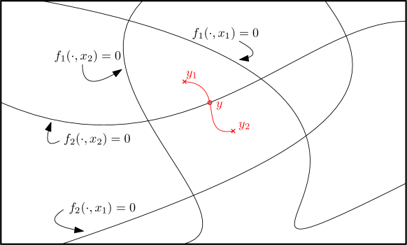
Figure 5: Illustration for the proof of Lemma 6.1: In this example $y_{1}$ and $y_{2}$ differ in $sgn(f_{2}(\cdot,x_{2}))$.

However, in general, it could happen that some ranges of ${\mathcal{R}}_{|A}$ can only be realized with a parameter $y$ such that $f_{i}(y,x_{j})=0$ for some $i$ and $j$. In this case, $y\notin S$. To prevent this, we define slightly shifted variations $f_{1}^{\prime},\dots,f_{t}^{\prime}$ of the functions $f_{1},\dots,f_{t}$ such that every $r\in{\mathcal{R}}_{|A}$ can be realized by some $y\in S^{\prime}$ where $S^{\prime}\coloneqq{\mathbb{R}}^{d}-\bigcup_{i=1}^{t}\bigcup_{j=1}^{m}\{y\in{\mathbb{R}}^{d}:f_{i}^{\prime}(y,x_{j})=0\}$. Let $|{\mathcal{R}}_{|A}|=N$ and $y_{1},\dots,y_{N}\in{\mathbb{R}}^{d}$ such that ${\mathcal{R}}_{|A}=\{r_{y_{1}},\dots,r_{y_{N}}\}$. Choose

$$\varepsilon=\frac{1}{2}\min\{|f_{i}(y_{l},x_{j})|:f_{i}(y_{l},x_{j})<0,1\leq i\leq t,1\leq j\leq m,1\leq l\leq N\}$$

and set $f_{i}^{\prime}(x,y)=f_{i}(y,x)+\varepsilon$ for all $i$. By construction, the sign values of all functions stay the same and none of them evaluates to zero for $y_{1},\dots,y_{N}$. Therefore the number of connected components of $S^{\prime}$ is at least $N$.

By bounding the number of connected components in the arrangement of Lemma 6.1 by $2(\frac{2emtl}{d})^{d}$ for every $t$-combination of $sgn(F)$, the bound in Theorem 1.1 implied using standard arguments (see [3] for details).

References

- [1] Peyman Afshani and Anne Driemel. On the complexity of range searching among curves. In Proceedings of the 2018 Annual ACM-SIAM Symposium on Discrete Algorithms (SODA), pages 898–917, 2018.
- [2] Hugo Akitaya, Frederik Brüning, Erin Chambers, and Anne Driemel. Subtrajectory Clustering: Finding Set Covers for Set Systems of Subcurves. Computing in Geometry and Topology, 2(1):1:1–1:48, Feb. 2023.
- [3] Martin Anthony and Peter L. Bartlett. Neural Network Learning: Theoretical Foundations. Cambridge University Press, 1999.
- [4] Shai Ben-David and Michael Lindenbaum. Localization vs. Identification of Semi-Algebraic Sets. In Lenny Pitt, editor, Proceedings of the Sixth Annual ACM Conference on Computational Learning Theory, COLT 1993, Santa Cruz, CA, USA, July 26-28, 1993, pages 327–336. ACM, 1993.
- [5] Frederik Brüning, Jacobus Conradi, and Anne Driemel. Faster Approximate Covering of Subcurves Under the Fréchet Distance. In Shiri Chechik, Gonzalo Navarro, Eva Rotenberg, and Grzegorz Herman, editors, 30th Annual European Symposium on Algorithms (ESA 2022), volume 244 of Leibniz International Proceedings in Informatics (LIPIcs), pages 28:1–28:16, Dagstuhl, Germany, 2022. Schloss Dagstuhl – Leibniz-Zentrum für Informatik.
- [6] Maike Buchin and Dennis Rohde. Coresets for ()-Median Clustering Under the Fréchet Distance. In Niranjan Balachandran and R. Inkulu, editors, Algorithms and Discrete Applied Mathematics, pages 167–180, Cham, 2022. Springer International Publishing.
- [7] Siu-Wing Cheng and Haoqiang Huang. Solving Fréchet distance problems by algebraic geometric methods. CoRR, abs/2308.14569, 2023.
- [8] Siu-Wing Cheng and Haoqiang Huang. Solving Fréchet distance problems by algebraic geometric methods. In Proceedings of the 2024 Annual ACM-SIAM Symposium on Discrete Algorithms (SODA), 2024. To appear.
- [9] Anne Driemel, André Nusser, Jeff M. Phillips, and Ioannis Psarros. The VC Dimension of Metric Balls under Fréchet and Hausdorff Distances. Discrete & Computational Geometry, 66(4):1351–1381, 2021.
- [10] Dan Feldman. Introduction to Core-sets: an Updated Survey. ArXiv, abs/2011.09384, 2020.
- [11] Dan Feldman and Michael Langberg. A Unified Framework for Approximating and Clustering Data. In Proceedings of the Forty-Third Annual ACM Symposium on Theory of Computing, STOC ’11, page 569–578, New York, NY, USA, 2011. Association for Computing Machinery.
- [12] Paul Goldberg and Mark Jerrum. Bounding the Vapnik-Chervonenkis dimension of concept classes parameterized by real numbers. In Lenny Pitt, editor, Proceedings of the Sixth Annual ACM Conference on Computational Learning Theory, COLT 1993, Santa Cruz, CA, USA, July 26-28, 1993, pages 361–369. ACM, 1993.
- [13] Paul W. Goldberg and Mark R. Jerrum. Bounding the Vapnik-Chervonenkis dimension of concept classes parameterized by real numbers. Machine Learning, 18:131–148, 1995.
- [14] Sariel Har-Peled and Micha Sharir. Relative (p, )-Approximations in Geometry. Discret. Comput. Geom., 45(3):462–496, 2011.
- [15] David Haussler and Emo Welzl. Epsilon-nets and simplex range queries. Discrete & Computational Geometry, 2(2):127–151, 1987.
- [16] Sarang Joshi, Raj Varma Kommaraji, Jeff M. Phillips, and Suresh Venkatasubramanian. Comparing Distributions and Shapes Using the Kernel Distance. In Proceedings of the Twenty-Seventh Annual Symposium on Computational Geometry, SoCG ’11, page 47–56, New York, NY, USA, 2011. Association for Computing Machinery.
- [17] Marek Karpinski and Angus Macintyre. Polynomial bounds for VC dimension of sigmoidal neural networks. In Proceedings of the Twenty-Seventh Annual ACM Symposium on Theory of Computing, STOC ’95, page 200–208, New York, NY, USA, 1995. Association for Computing Machinery.
- [18] Michael Lindenbaum and Shai Ben-David. Applying VC-dimension analysis to 3D object recognition from perspective projections. In Barbara Hayes-Roth and Richard E. Korf, editors, Proceedings of the 12th National Conference on Artificial Intelligence, Seattle, WA, USA, July 31 - August 4, 1994, Volume 2, pages 985–990. AAAI Press / The MIT Press, 1994.
- [19] Michael Lindenbaum and Shai Ben-David. Applying VC-dimension analysis to object recognition. In Jan-Olof Eklundh, editor, Computer Vision - ECCV’94, Third European Conference on Computer Vision, Stockholm, Sweden, May 2-6, 1994, Proceedings, Volume I, volume 800 of Lecture Notes in Computer Science, pages 239–250. Springer, 1994.
- [20] Vladimir N. Vapnik. The Nature of Statistical Learning Theory. Springer New York, NY, 2000.
- [21] Vladimir N. Vapnik and Alexey Ya. Chervonenkis. On the uniform convergence of relative frequencies of events to their probabilities. Theory of Probability & Its Applications, 16(2):264–280, 1971.