Probabilistic Neural Transfer Function Estimation with Bayesian System Identification

Abstract

Neural population responses in sensory systems are driven by external physical stimuli. This stimulus-response relationship is typically characterized by receptive fields, which have been estimated by neural system identification approaches. Such models usually requires a large amount of training data, yet, the recording time for animal experiments is limited, giving rise to epistemic uncertainty for the learned neural transfer functions. While deep neural network models have demonstrated excellent power on neural prediction, they usually do not provide the uncertainty of the resulting neural representations and derived statistics, such as the stimuli driving neurons optimally, from in silico experiments. Here, we present a Bayesian system identification approach to predict neural responses to visual stimuli, and explore whether explicitly modeling network weight variability can be beneficial for identifying neural response properties. To this end, we use variational inference to estimate the posterior distribution of each model weight given the training data. Tests with different neural datasets demonstrate that this method can achieve higher or comparable performance on neural prediction, with a much higher data efficiency compared to Monte Carlo dropout methods and traditional models using point estimates of the model parameters. At the same time, our variational method allows to estimate the uncertainty of stimulus-response function, which we have found to be negatively correlated with the predictive performance and may serve to evaluate models. Furthermore, our approach enables to identify response properties with credible intervals and perform statistical test for the learned neural features, which avoid the idiosyncrasy of a single model. Finally, in silico experiments show that our model generates stimuli driving neuronal activity significantly better than traditional models, particularly in the limited-data regime. Together, we provide a probabilistic approach for identifying neuronal representation with full distribution, which may help uncover the underpinning of high-dimensional biological computation.

1 Introduction

Current neural interfaces allow to simultaneously record large populations of neural activity. In sensory neuroscience, such ensemble responses are driven by external physical stimuli (e.g., natural images), and their relation has been characterized by tuning curves or receptive fields (RFs; Hubel and Wiesel (1959)). Such stimulus-response functions have been estimated by neural system identification methods (reviewed in Wu et al., 2006). Classically, they used a linear-nonlinear-Poisson (LNP) model or variants of it (Chichilnisky, 2001; Pillow et al., 2008; Huang et al., 2021; Karamanlis and Gollisch, 2021) to predict responses to unseen stimuli such as white noise and natural images (Rust and Movshon, 2005; Qiu et al., 2021). More recently, deep neural networks (DNNs) with multiple layers of non-linear processing have shown great success for learning neural transfer functions along the ventral visual stages from retina (Qiu et al., 2023; McIntosh et al., 2016; Batty et al., 2016) and primary visual cortex (Antolík et al., 2016; Klindt et al., 2017; Ecker et al., 2018; Lurz et al., 2021) to higher visual areas (Yamins et al., 2014; Güçlü and van Gerven, 2015). Moreover, through in silico experiments, these models are able to generate specific stimulus to control neural activity and identify novel neuronal properties from a high-dimensional space (Bashivan et al., 2019; Ponce et al., 2019; Walker et al., 2019; Franke et al., 2021; Hoefling et al., 2022). For example, closed-loop paradigms show that performing gradient ascent on a deep model can yield most exciting inputs (MEIs) to drive a neuron’s activity optimally (Walker et al., 2019; Tong et al., 2023).

Yet, these system identification approaches demand significant amounts of stimulus-response pair data for the model training, given the high dimensional stimulus space and the non-linear neural transformations (Qiu et al., 2023; Lurz et al., 2021; Cotton et al., 2020). Due to limited recording time for each experiment, the amount of data for fitting these models is restricted introducing epistemic uncertainty about the learned stimulus-response function. To estimate this uncertainty, traditional LNP methods obtain full posterior distribution of model parameters by leveraging a Bayesian framework to provide confidence intervals for the estimated RFs (Gerwinn et al., 2007, 2010; Park and Pillow, 2011; Huang et al., 2021). However, DNN models rarely consider the uncertainty of the neuronal properties that are recovered from in silico experiments.

Here, we propose a Bayesian system identification approach to estimate response features of neurons with uncertainties (Figure 1). We test whether incorporating uncertainties by learning the full distribution of model parameters is beneficial for learning neural representations. To this end, we build a DNN model to predict responses to unseen visual stimuli by using variational inference to estimate the distribution of network weights, i.e., Bayes by Backprop (Hinton and Van Camp, 1993; Neal and Hinton, 1998; Jaakkola and Jordan, 2000; Blundell et al., 2015).

Our contributions are: (1) We incorporate weight variability in deep neural networks for identifying neural response functions with uncertainty and extend the Bayes by Backprop with a hyperparameter which effectively adjusts the sparsity of model parameters. (2) We apply our Bayesian models on different experimental datasets and find that our method can achieve higher or comparable performance on neural prediction, with a much better data efficiency, compared to Monte Carlo dropout methods and traditional models using point estimates of the model parameters. (3) Our approach with full posterior allows to estimate neural features with credible intervals and run statistical test for the derived MEIs, bypassing the idiosyncrasy of a single model. (4) Finally, simulation experiments demonstrate that the variational model yields stimuli that drive neuronal activation better than the traditional models, especially in the condition of limited training data. This supports that weight uncertainty, as implemented in our model, may contribute to a more efficient identification of non-linear neuronal response functions.

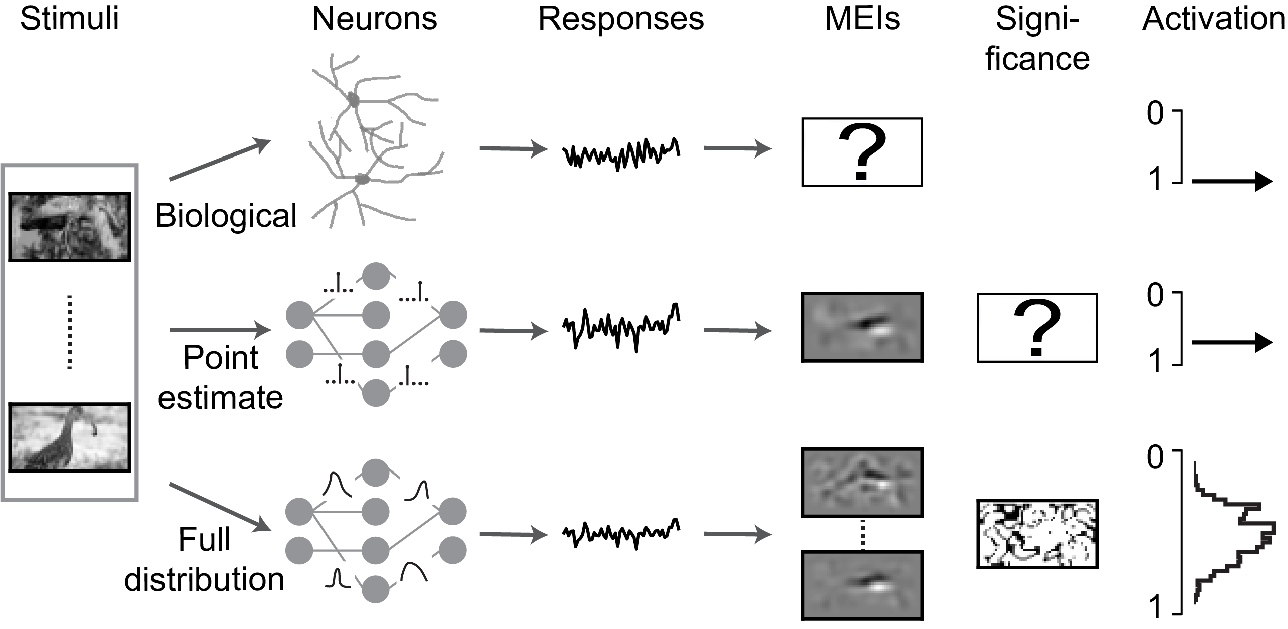
Figure 1: Schematic of neural system identification for predicting responses. Biological neurons (top row; second column) respond to visual stimuli (first column) distinctly (third column), with an unknown MEI (fourth column) driving a cell with optimal activation (sixth column). Traditional system identification methods (center row) learn stimulus-response function and yield a MEI with unknown statistics (fitth column). Bayesian approaches (bottom row) learn distributions of model parameters to predict neuronal responses, yielding an infinite MEIs, whose significance map can be computed by sampling from posterior, to drive a neuron with credible intervals.

2 Materials and methods

2.1 Models

Variational model

DNN for system identification can be seen as a probabilistic model: given the training data $\mathcal{D}=(\textbf{x}_{i},\textbf{y}_{i})_{i}$ where $\textbf{x}_{i}$ is an input (such as natural images) and $\textbf{y}_{i}$ is the output (such as neural responses), we aim to learn the weights w of a network which can predict the output for the unseen stimuli (Figure 1). Compared to a traditional method using point estimates of the weights, Bayesian approaches learn full distributions of these w. Estimating the full posterior distribution of the weights $P(\textbf{w}|\mathcal{D})$ given the training data is usually not feasible. An alternative is to approximate $P(\textbf{w}|\mathcal{D})$ by a new distribution $q(\textbf{w}|\theta)$ whose parameters $\theta$ are trained to minimize the distance between the proxy and the true posterior, which is called variational inference (Hinton and Van Camp, 1993; Neal and Hinton, 1998; Jaakkola and Jordan, 2000; Blundell et al., 2015). Usually we use Kullback-Leibler (KL) divergence as a measure of distance between two distributions:

$$\theta^{*} =\operatorname*{arg\,min}_{\theta}\textbf{KL}[q(\textbf{w}|\theta)||P(\textbf{w}|\mathcal{D})]$$ (1)

$$=\operatorname*{arg\,min}_{\theta}\textbf{KL}[q(\textbf{w}|\theta)||P(\textbf{w})]-\operatorname{\mathbb{E}}_{q(\textbf{w}|\theta)}[\log P(\mathcal{D}|\textbf{w})]$$ (2)

The optimization function can be viewed as a trade-off between the distance between the variational posterior and the selected prior and the likelihood cost. We can view it as a constrained optimization problem as (Higgins et al., 2016):

$$\operatorname*{arg\,max}_{\theta}\operatorname{\mathbb{E}}_{q(\textbf{w}|\theta)}[\log P(\mathcal{D}|\textbf{w})]\;\;\;\;\text{subject to}\;\;\textbf{KL}[q(\textbf{w}|\theta)||P(\textbf{w})]<\epsilon$$ (3)

Here $\epsilon$ represents the specific distance between the variational posterior and the prior. According to KKT conditions (Kuhn and Tucker, 1951) and non-negative properties of KL divergence, we get:

$$\mathcal{F} =\operatorname{\mathbb{E}}_{q(\textbf{w}|\theta)}[\log P(\mathcal{D}|\textbf{w})]-\beta_{v}(\textbf{KL}[q(\textbf{w}|\theta)||P(\textbf{w})]-\epsilon)$$ (4)

$$\geq\operatorname{\mathbb{E}}_{q(\textbf{w}|\theta)}[\log P(\mathcal{D}|\textbf{w})]-\beta_{v}\textbf{KL}[q(\textbf{w}|\theta)||P(\textbf{w})]$$ (5)

where $\beta_{v}$ is non-negative and represents a Lagrangian multiplier. So the final loss function for the model is:

$$\mathcal{L} =\beta_{v}\textbf{KL}[q(\textbf{w}|\theta)||P(\textbf{w})]-\operatorname{\mathbb{E}}_{q(\textbf{w}|\theta)}[\log P(\mathcal{D}|\textbf{w})]$$ (6)

$$\approx\sum_{i=1}^{n}\beta_{v}(\log q(\textbf{w}^{(i)}|\theta)-\log P(\textbf{w}^{(i)}))-\log P(\mathcal{D}|\textbf{w}^{(i)})$$ (7)

Eq. (7) is a result of Monte Carlo sampling $n$ instances $\textbf{w}^{(i)}$ from $q(\textbf{w}|\theta)$ because we can not calculate (6) directly.

Here, we implemented convolutional neural networks (CNNs) for all experiments. For a CNN using variational inference on model weights (variational model), we picked independent Gaussian distributions for the variational posterior and a scale mixture of two Gaussians for the prior (Blundell et al., 2015). The log posterior was defined as $\log q(\textbf{w}|\theta)=\sum_{k=1}\log\mathcal{N}(w_{k}|\mu,\sigma^{2})$ where $w_{k}$ denotes $k$th weight of the neural network and $(\mu,\sigma)$ are the posterior parameters $\theta$. To keep $\sigma$ non-negative, we parameterised it using $\sigma=\log(1+\exp{(\rho)})$. We selected the log prior $\log P(\textbf{w})=\sum_{k=1}\log(\pi\mathcal{N}(w_{k}|0,\sigma_{1}^{2})+(1-\pi)\mathcal{N}(w_{k}|0,\sigma_{2}^{2}))$ where $\pi$ is a mixture component weight ($0\leq\pi\leq 1$) (Blundell et al., 2015; Fortuin et al., 2021). This prior, compared to a single Gaussian distribution, encourages sparseness in learned kernels, reminiscent of neural representations in visual systems (Field, 1994; Olshausen and Field, 1996; Olshausen and Millman, 1999; Stevenson et al., 2008). The likelihood loss depends on the specific task of the network. For neural system identification, we use Poisson loss $-\log P(\mathcal{D}|\textbf{w})=\sum_{l}\hat{\textbf{r}}_{l}-{\textbf{r}_{l}}\log\hat{\textbf{r}}_{l}$, where $l$, $\hat{\textbf{r}}_{l}$ and ${\textbf{r}_{l}}$ denote neuronal index, prediction responses and true responses, respectively.

Baseline and control models

We used a CNN without any regularization as a baseline model (Appendix 5.1) and used a CNN with L2 regularization in each convolutional layer and L1 regularization in fully connected layer (L2+L1) as a control model. We adopted an ensemble of L2+L1 models with different initialization seeds as a second control model, whose predicted responses are the average of five model outputs. To examine the contribution from weight uncertainties, we built a maximum a posteriori (MAP) model which contains prior and likelihood terms in Eq. (7) as loss functions. Additionally, as a fourth control, we adopted a CNN with Monte Carlo dropout for probabilistic prediction; it used the same dropout rate for each model layer and in both training and test stages (Srivastava et al., 2014; Gal and Ghahramani, 2016).

2.2 Dataset

We tested our method on two publicly available datasets.

The first dataset contains calcium signals driven by static natural gray-scale images for neurons in primary visual cortex (V1) of mice (Antolík et al., 2016). We used 103 neurons from the first scan field, whose single-trial responses to 1,600 images for training models and 200 for tuning hyperparameters. Then we used the mean of response repeats to 50 test images for evaluating models.

The second dataset comprises Ca^2+ responses to natural green/UV images (36x64 pixels) for neurons in mouse V1 (Franke et al., 2021). We selected the natural stimuli that were presented in both UV and green channels and used the neurons whose quality index ($QI=\mathrm{Var}[\mathrm{E}[C]_{r}]_{t}/\mathrm{E}[\mathrm{Var}[C]_{t}]_{r}$, time samples $t$ and repetitions $r$, a response matrix $C$ with a shape of $t\times r$, $\mathrm{E}[X]_{d}$ and $\mathrm{Var}[X]_{d}$ denoting the mean and variance along the dimension $d$ of $X$, respectively) of 10-repeat test responses were larger than 0.3. In this way, we had 161 neurons from one scan field, whose single-trial responses to 4,000 images for training and 400 for validation. Then we used mean of response repeats to 79 test images for evaluation.

2.3 Training and evaluation

We trained all models with a learning rate of 0.0003 for a maximum of 200 epochs using the Adam optimizer (Kingma and Welling, 2013). We computed linear correlation (correlation coefficient, CC) between predicted and recorded responses, which was used to evaluate models on validation or test data. We tuned model hyperparameters and selected the ones as well as the respective epoch number with the best predictive performance on validation data. To keep the comparison fair, the test models shared similar network architecture for each dataset, except that the dropout model featured dropout layers.

For each trained model, we estimated MEIs of all neurons by running gradient ascent on a random input image for 100 steps with a learning rate of 10 and we picked the stimulus with the highest activity (Erhan et al., 2009; Walker et al., 2019). All generated MEIs had the same mean and standard deviations as the training images. For the two probabilistic (variational and dropout) models, we ran the estimation for 100 times with Monte Carlo sampling, hence, we got 100 MEIs (matrix $C$) for each recorded neuron. Note that we fixed the random seed/state for each sampling, in this way, model weights did not change stochastically during the iterative generation of each MEI. We defined MEI variance of one neuron as $\mathrm{MEI\;variance}=\mathrm{E}[\mathrm{Var}[C]_{s}]_{hw}$ (sampling times $s$, stimulus height $h$, stimulus width $w$, and $C$ with a shape of $s\times h\times w$). The overall MEI variance for a model was an average of MEI variances for the recorded neurons.

In in silico experiments, to measure the activation distribution of MEIs yielded from variational models for a neuron, we estimated 100 MEIs by sampling and one mean MEI by using the weight mean $\mu$ from each seed. So we had 505 MEIs for five random seeds with one additional MEI which was the mean of the five mean MEIs, in total 506 MEIs. For L2+L1 models, we estimated five MEIs from different random seeds and also got one by averaging across these MEIs, in total 6 MEIs.

3 Results

3.1 $\beta_{v}$ balances model capacity and data likelihood

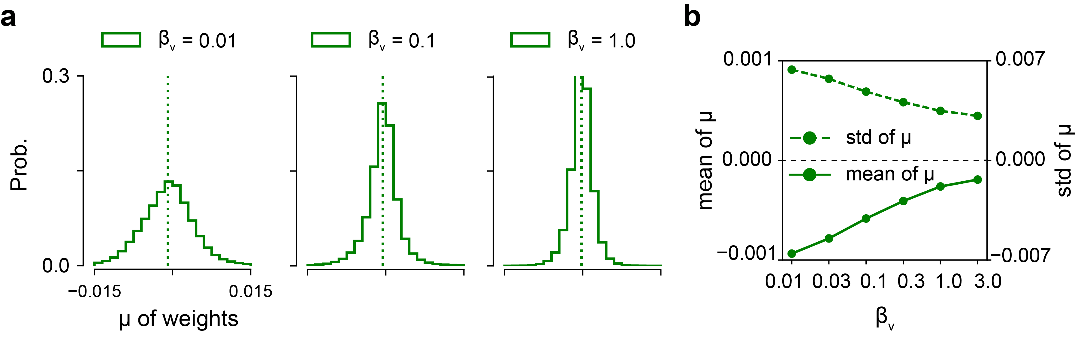
Figure 2: Hyperparameter $\beta_{v}$ for regulating weight sparseness. (a) Distribution of the means ($\mu$) of model weights for different $\beta_{v}$ values. Dotted lines indicate distribution means. (b) Mean and standard deviation for the distributions in (a).

Compared to a conventional evidence lower bound in Eq. (2), we used a Lagrangian multiplier $\beta_{v}$ in (7) by borrowing the idea of constrained optimization from Higgins et al. (2016). In this way, Blundell and colleague’s work can be seen as a special case of $\beta_{v}=1.0$ (Blundell et al., 2015). We first analyzed the possible roles of $\beta_{v}$. We investigated it from the perspective of information theory, given that Eq. (7) has a similar form with the objective functions in deep variational information bottleneck (Alemi et al., 2016; Tishby et al., 2000) and $\beta$-VAE (Higgins et al., 2016; Burgess et al., 2018).

The training objective jointly minimizes the KL divergence between the posterior $q(\textbf{w}|\theta)$ and the prior $P(\textbf{w})$ and maximizes the data likelihood under the distribution $q(\textbf{w}|\theta)$. The distribution distance becomes zero when $q(\textbf{w}|\theta)=P(\textbf{w})$. In the case of Gaussian posterior and mixture-of-Gaussians prior with mean zero (e.g., a distribution with $\pi=0.5,\sigma_{1}=1,\sigma_{2}=\exp{(-6)}$), the divergence decreases with the posterior mean moving close to zero and the posterior variance decreasing (as the exemplary prior has around 50% of chance to be zero), which induces many zeros for weights w and increases the sparsity of model parameters. In the extreme case, all weights are equal to zeros and the model does not have any expressive power. In such case, the log likelihood $\operatorname{\mathbb{E}}_{q(\textbf{w}|\theta)}[\log P(\mathcal{D}|\textbf{w})]$ vanishes, indicating that the posterior $q(\textbf{w}|\theta)$ is a bottleneck for maximizing the data likelihood. Therefore, $\beta_{v}$ can be interpreted as a coefficient to adjust model expressive power for fitting the data.

Empirically, we examined the distribution of weight means ($\mu$) for different $\beta_{v}$ values on the dataset 1 shared by by Antolik and colleagues (Antolík et al., 2016). Indeed, we found that with the increase of $\beta_{v}$, the mean of the distribution got close to zeros and the standard deviation decreased, indicating an increase of sparsity of model weights (Fig. 2). Similarly, we measured the percentage of the weights with absolute values below certain threshold ($0.005$) and also observed an increase of the ratio (data not shown). Therefore, the hyperparameter $\beta_{v}$ served to tune the model capacity via weight sparseness for data prediction.

3.2 System identification incorporates model uncertainty to predict neural responses

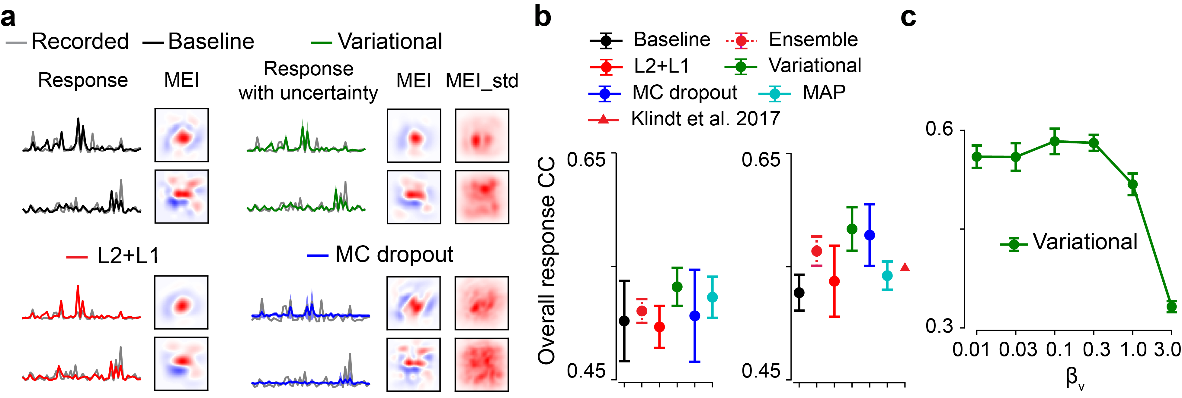
Figure 3: Neural prediction with weight uncertainty. (a) Mean recorded responses (gray) and predictive responses to natural stimuli(black, baseline; red, L2+L1; green, variational one with $\beta_{v}=0.1$; blue, MC dropout with dropout rate 70%; shaded green and blue representing standard deviation for the variational and the dropout methods, respectively), estimated MEIs, as well as standard deviation of MEI (MEI_std; only for two probabilistic models), for two exemplary neurons. MEI and MEI_std use different color scales with red and blue indicating positive and negative values, respectively. Note that MEI has much larger absolute values than MEI_std. (b) Predictive performance based on test data with different amounts of training data (left, 50% of training data; right, 100% of data) for 6 models (red dash, ensemble; cyan, MAP; 10 seeds per model), and the one used by (Klindt et al., 2017) (red triangle). (c) Predictive model performance for different $\beta_{v}$ values. Error bars in (b) and (c) represent standard deviation of n=10 random seeds for each model.

We trained the six models on the dataset 1 (Fig. 3a) and tuned their respective hyperparameters using validation data. For the variational model, we found the one with $\beta_{v}=0.1$ had best predictive performance with a sharp decrease when increasing $\beta_{v}$ till 1.0 or 3.0 (Appendix 5.2.1). We also observed that at training stage, the variational model presented a more stable performance on validation data compared to the baseline CNN, confirming the regularization effect of prior to prevent overfitting.

Next, we selected the hyperparameters achieving the best performance on validation data for each model. To examine the feature properties learned by these models, we estimated the MEIs of recorded neurons and found that these models yielded antagonistic center-surround and Gabor filters in a local region, reminiscent of neural representations in early visual processing ((Hubel and Wiesel, 1959; Chichilnisky, 2001); Fig. 3a). To compare the performance of neural prediction, we then evaluated all models using test data. For a probabilistic model, we ran model predictions for 100 sampling times and computed the mean and the standard deviation of neuronal responses. Interestingly, when we used the full training data, the variational and MC dropout models had similar predictive performance ($p=0.6159$, two-sided permutation test with n = 10,000 repeats). The variational one also outperformed the baseline, the L2+L1, the ensemble, the MAP ($p=0.0001$) and the model with shared feature space between neurons((Klindt et al., 2017); Fig. 3b). With half of training data, the variational method yielded a correlation slightly/non-significantly higher compared to the MC dropout method ($p=0.082$). The performance difference between variational and traditional methods using point estimates of parameters indicates the benefit of weight uncertainty for neural prediction. We then reanalyzed the influence of $\beta_{v}$ on prediction for the variational model using test data. Similar to the case with validation data, we noticed a rather steady predictive performance with increasing $\beta_{v}$ until a sudden drop at $\beta_{v}=1.0$ or 3.0, implying that a large Lagrangian multiplier imposing excessive sparsity on weights yields model underfitting.

Together, the superior/equivalent performance of our variational approach suggests that incorporating weight uncertainty is beneficial for predicting neural responses.

3.3 Probabilistic models learn variance of neural transfer functions

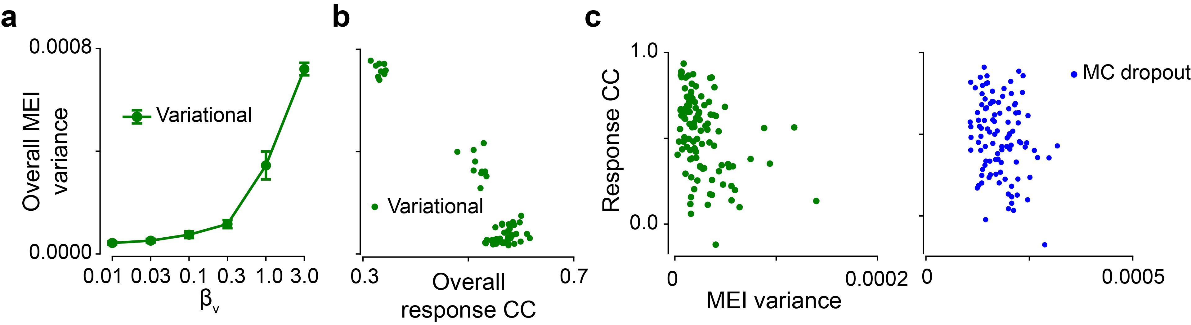
Figure 4: Neural transfer functions with variability. (a) Overall MEI variance for different $\beta_{v}$ values (10 seeds per model). (b) Scatter plot of overall response CC and overall MEI variance for 6 $\beta_{v}$ values and 10 seeds (each dot representing one model at each $\beta_{v}$ and each seed). (c) Scatter plot of response CC and MEI variance for two probabilistic models at one random seed (each dot representing one neuron). Error bars in (a) represent standard deviation of n=10 random seeds for each model.

The variational and the MC dropout approaches enable us to learn stimulus-response functions with credible intervals. We next asked whether the variability of the learned transfer function was related to the predictive performance for the two probabilistic (variational and dropout) models. To this end, we measured the MEI variance for each neuron and the overall MEI variance for each model and relate them to the performance on predicting responses.

We first investigated the influence of $\beta_{v}$ on the variability of the learned transfer functions for our variational model. Interestingly, we found a sudden increase of overall MEI variance at $\beta_{v}=1.0$ or $3.0$ (Fig. 4a), where an abrupt drop of model performance was present (cf. Fig. 3c). This opposite change between MEI variability and predictive performance was confirmed by the negative correlations between overall MEI variance and overall response CC ($CC=-0.95,p<0.0001$; Fig. 4b). Additionally, this negative correlation was also reflected at neuronal level. Both the variational and the MC dropout models had a negative correlation between response CC and MEI variance for the recorded neurons ($CC=-0.37,p=0.0001$ and $CC=-0.23,p=0.02$ for the variational and the MC dropout, respectively; Fig. 4c), indicating that, for a trained probabilistic model, neurons with higher predictive performance have higher confidence on its estimated MEI.

In summary, these results demonstrate that a probabilistic model with smaller uncertainty on the learned stimulus-response function yields higher predictive performance.

3.4 Variational model features high data efficiency on neural prediction

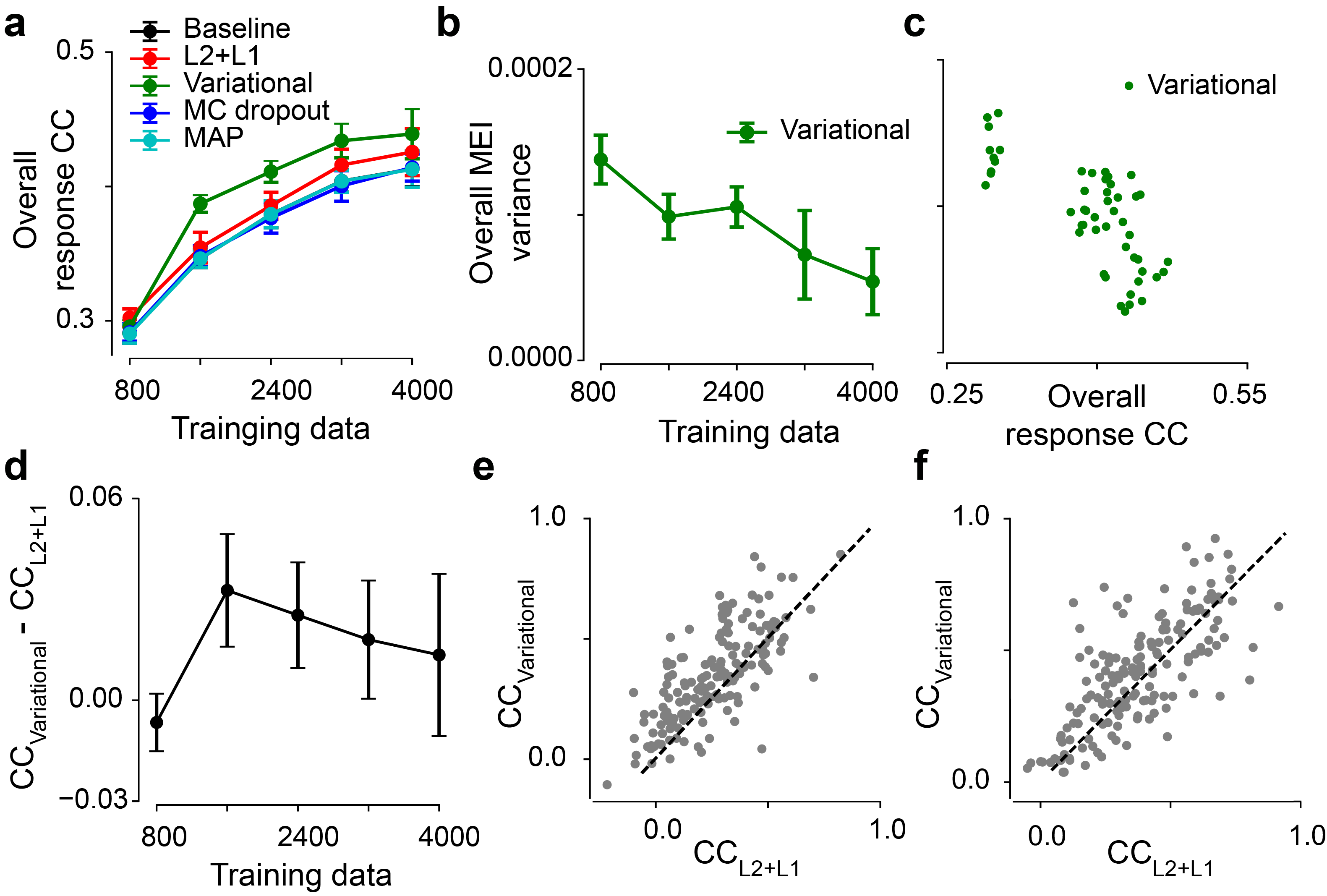
Figure 5: Variational models on the second dataset. (a) Model performance based on test data of the second dataset with different amounts of training data for five models (n=10 random seeds per model). (b) Overall MEI variance for different amounts of training data for variational models (10 seeds per model). (c) Scatter plot for overall response CC and overall MEI variance for different amounts of training data and at 10 seeds. Each dot representing one model. (d) Performance difference between the variational and the L2+L1 models. (e) Scatter plot of model predictions for the variational model and the L2+L1 model at one random seed when using 40% training data. Each dot representing one neuron. (f) Like (e) but using 100% training data. Error bars in (a), (b) and (d) represent standard deviation of n=10 random seeds for each model.

Here we applied our method on the second dataset shared by Franke and colleagues ((Franke et al., 2021)). After hyperparameter tuning, we selected $\beta_{v}=0.3$ for the variational network and evaluated the five models on test data.

We first examined the relationship between the uncertainty of the learned stimulus-response function and the performance on predicting responses. We expect that, with more data used for training, the model yields better prediction along with smaller variance for the learned MEIs. We focused on the variational method. Indeed, when more training data was used, the predictive model performance increased (Fig. 5a) while the overall MEI variance decreased Fig. 5b, with a negative correlation between them ($CC=-0.73,p<0.0001$; Fig. 5c). Note that we did not observe a steady decrease of the overall response variance (Appendix 5.2.2).

Next, we investigated whether the performance difference between the variation and the L2+L1 model was sensitive to the training data size (Fig. 5d). We observed that the variational method had higher correlations except for the case of extremely little data (20%). The difference peaked at 40% with an increase of 9% ($p<0.0001$, two-sided permutation test with n = 10,000 repeats) and gradually decreased with more training data, indicating the benefit of variational inference for system identification. We also compared the predictive performance on individual neurons at one random seed, the Bayesian model outperformed the L2+L1 one for the conditions of 40% ($p<0.0001$) and 100% (non-significantly; $p=0.0927$) training data.

Together, compared to a traditional method, our Bayesian approach with weight uncertainty yielded higher predictive performance with a higher data efficiency.

3.5 Variational model yields stimuli driving high neuronal activation

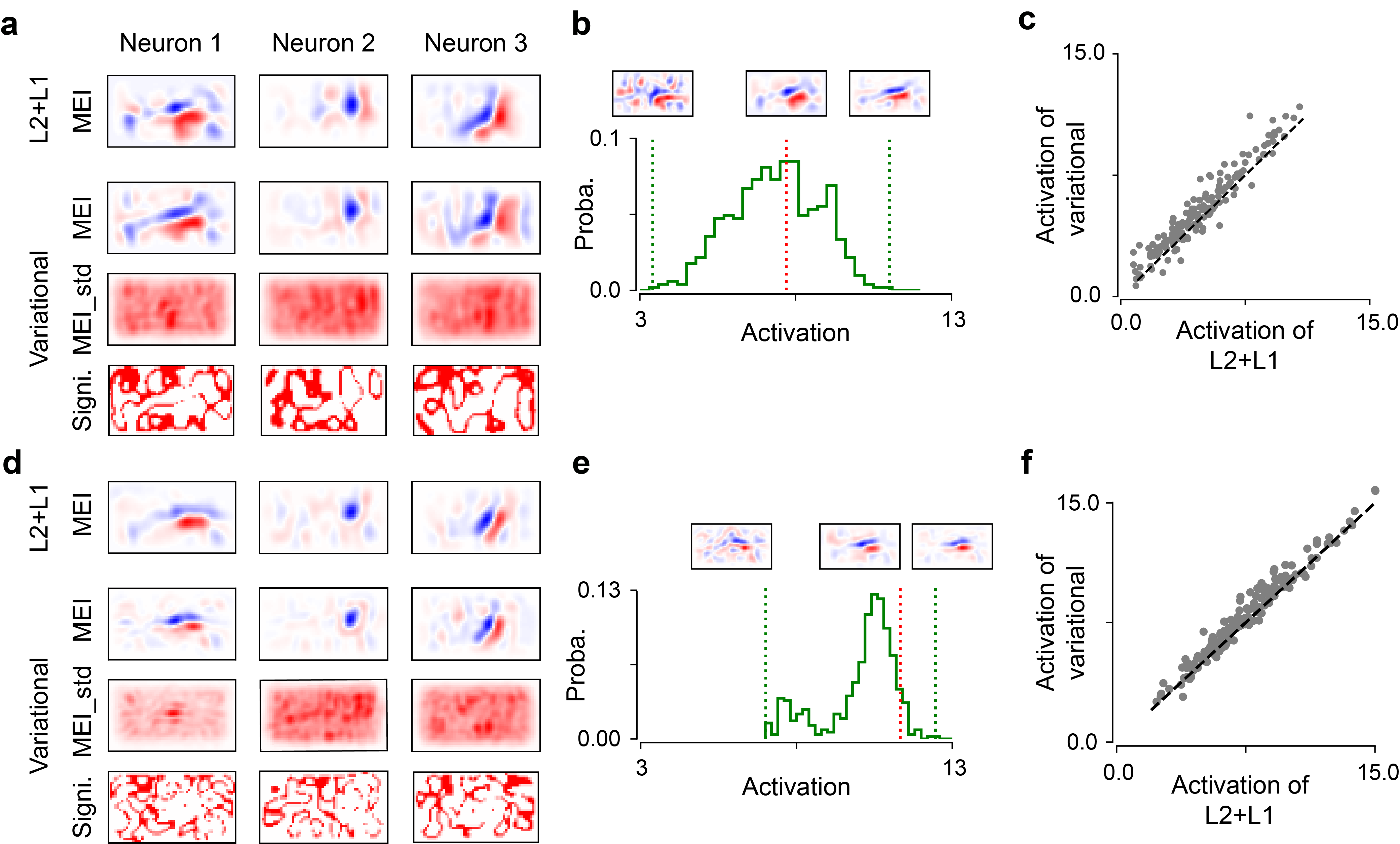
Figure 6: In silico experiments of neuronal activity with derived MEIs. (a) Estimated MEIs for L2+L1 (first row) and variational (second row) models, MEI_std (third row), as well as significance map (fourth row; white, $p<0.01$, one-sample two-sided permutation test against zero for 10,000 repeats), for three exemplary neurons when using 40% of training data. MEI and MEI_std in the UV channel, with different color scales. Note that MEI has much larger absolute values than MEI_std. (b) 1D histogram of neuronal activity driven by the generated MEIs from the variational model for Neuron 1 when using 40% of training data. Insets: example MEIs with corresponding activation indicated by dotted lines (red, maximum of L2+L1; green, variational). (c) Scatter plot of activation driven by MEIs yielded from variational (using the weight mean $\mu$) and L2+L1 models at one random seed when using 40% of training data. Each dot representing one cell. (d,e,f) Same with (a), (b) and (c), but using 100% of training data.

Bayesian methods with full posterior provide an infinite ensemble of models for computing MEIs and allow to perform statistical tests for the derived features. We focused on the model using variational inference and the one using L2 and L1 regularization with 40% and 100% of training data. We found that these learned filters resembled neural features in the early visual system (Hubel and Wiesel, 1959; Chichilnisky, 2001) and localized more in the visual field with more training data (Fig. 6a,d). Like for the first dataset (Fig. 3a), MEI_std was not uniform across visual space, e.g., some presented Gaussian or bar shapes. Additionally, we examined whether the posterior of each pixel differs significantly from zero for the 100 sampled MEIs and found that the significance map may indicate zero-crossings in visual representations.

To examine the effectiveness of our variational approach, we fed the verified MEIs from Franke et al. (2021) into the model trained by full data and estimated the neuronal activation. Indeed, we observed that each cell was driven most by its respective preferred stimulus (Appendix 5.2.4).

To further assess which method generates the more exciting stimuli for each cell, we conducted in silico experiments using a held-out L2+L1 model trained by full data as a digital testbed. We used a CNN model with regularization instead of other models as previous studies have demonstrated its feasibility on yielding cells’ preferred stimuli (Walker et al., 2019; Franke et al., 2021; Hoefling et al., 2022; Tong et al., 2023). For an example neuron, we measured the responses for all the 506 MEIs yielded from five variational models, and observed that these stimuli drove this neuron with quite different activity, with the maximum response larger than the maximum one yielded (from 6 MEIs) by the traditional models (Fig. 6b,e). With more training data, the activation distribution shifted towards higher mean with smaller variance. Additionally, we compared the activation on individual neurons for two methods (Fig. 6c,f), and observed that the Bayesian approach yielded significantly higher responses for the condition using 40% of training data ($p=0.0473$ and $p=0.2114$ for 40% and 100% of data, respectively; two-sided permutation test with n = 10,000 repeats).

In summary, our variational model allowed statistical test for the derived response functions and yielded the stimuli driving neurons better than traditional methods, suggesting that weight uncertainty benefits the learning of neural representations.

4 Discussion

We presented a Bayesian approach for identification of neural properties by incorporating model uncertainty through learning the distribution of model weights, aiming to estimate neural features with credible intervals. Our empirical results on different datasets show that the variational method had higher or comparable predictive performance, especially in the limited data regime, compared to methods using dropout or traditional methods learning point estimates of model parameters. Moreover, by sampling from posterior distribution of model weights, our approach enabled to provide credible intervals and test statistics for the learned MEIs, avoiding the idiosyncrasy of a single model. Finally, in silico experiments show that the variational model yielded the MEIs driving neurons with higher activity compared to the traditional model, in particular when limited data were used for training. This suggests that model uncertainty contributes to learning neural transfer functions with a high data efficiency.

4.1 Relation to trial-to-trial variability

Neural information process is probabilistic, i.e., neurons respond with trial-to-trial fluctuations to a repeated presentation of a stimulus (Perkel et al., 1967; Stein, 1967). Response variability is found across neural systems, originating from diverse factors, such as synapse variation, channel noise, brain state, and attention (Faisal et al., 2008; Mitchell et al., 2009; Cohen and Newsome, 2008; Cohen and Maunsell, 2009; Ecker et al., 2010, 2014). Additionally, the variability between populations of neurons are correlated. In a simplified case, a pair of neurons may present correlations for the single-trial responses, i.e., pairwise noise correlation, which also contributes to neural coding ((Abbott and Dayan, 1999); reviewed in (Averbeck et al., 2006; Kohn et al., 2016; Doiron et al., 2016; Da Silveira and Rieke, 2021)). Such response variability is inherent in neural data itself and is a kind of aleatoric, but not the epistemic uncertainty. We note that the standard deviations of the estimated MEIs from our models decreased with the increasing amounts of training data, suggesting that the variability of the sampled predicted responses may not be related to the response uncertainty in biological neurons or our models may predict a mix of both uncertainties (Appendix 5.2.3).

We did not observe a negative correlation between the predictive performance and the variance of predicted responses (cf. MEI variance; Appendix 5.2.1, 5.2.2), which might be related to the differential response variability driven by distinct stimuli (Goris et al., 2014; Ecker et al., 2014). This also suggests a future study to compare between the uncertainty of recorded and predicted responses and investigate the response variance from different models (such as variational inference vs. MC dropout). Additionally, it might be interesting to use proper scoring rules, e.g., Continuous Ranked Probability Score, to evaluate the quality of predictive uncertainty for the Bayesian models (Matheson and Winkler, 1976; Gneiting and Raftery, 2007).

4.2 Necessity of uncertainty quantification for yielded preferred stimuli

Though DNN approaches have demonstrated remarkable power in predicting neural responses to diverse stimuli and generating novel hypothesis about neuronal features, they require significant amounts of stimulus-response pair data for the training. Besides the epistemic uncertainty introduced by limited data, such hypothesis also entails further closed-loop animal experiments to verify the derived properties, which consumes much experimental time (Walker et al., 2019; Tong et al., 2023). Still, it is impossible to confirm the yielded preferred stimuli for all neurons across the high-dimensional stimulus space with experiments. Practically, only a subset of cells are selected for verification. Therefore, it is critical to quantify the uncertainty of the yielded representations for all recorded neurons (Richards et al., 2019; Saxe et al., 2021). Additionally, the credible interval of the derived features offers an opportunity to generate an ensemble of infinite preferred stimuli. An interesting study would be to compare the neuronal activity driven by these similar MEIs in animal experiments, which may allow to test the robustness of the biological system.

We note that, even for a model using point estimate of parameters (such as L2+L1), it may yield different preferred stimuli by initializing the MEI generation randomly. Yet, this uncertainty depends on the starting points of non-convex optimizations, rather than the training data. Empirically, we found that such variance was quite stable when using L2+L1 models with different amounts of training data and was also much smaller than the MEI variance we computed (cf. Fig. 5b). Therefore, the measure of epistemic uncertainty calls for a Bayesian framework or an ensemble of many models.

4.3 Future work & general impact

Incorporating uncertainty to DNNs have flourished in recent years (reviewed in Abdar et al., 2021; Gawlikowski et al., 2023), including Bayesian methods which specify a prior distribution for network weights and approximate the full posterior given the training data using different tricks such as variational inference (Blundell et al., 2015; Posch and Pilz, 2020), Laplace approximation (Mackay, 1992; Ritter et al., 2018) and expectation propagation (Li et al., 2015). Non-Bayesian methods include applying MC dropout in the network (Gal and Ghahramani, 2016) or training an ensemble of models that are initialized by different seeds (Lakshminarayanan et al., 2017). While these methods are powerful to predict uncertainty, it would be interesting to investigate biologically inspired methods such as adding noise to network parameters/activation in the future. Specifically, our variational approach incorporating model uncertainty did not predict the trial-to-trial variability. Such response fluctuation depends on many conditions, including biochemical process, internal brain states and engaged behavioral tasks (Faisal et al., 2008; Mitchell et al., 2009; Ecker et al., 2014; Goris et al., 2014). These factors have been described by a low-dimensional latent state models (Yu et al., 2008; Ecker et al., 2014; Bashiri et al., 2021). Therefore, a potential extension of our method could be a variational network incorporated with latent state variables.

Our in silico experiments indicate that the stimuli generated by the variation model driving higher neuronal activation than the CNN with regularization, which requires future animal experiments to test. Additionally, we noticed that the MEI_std was not uniform in the visual field for each neuron and its location was not overlaid with the central MEI, for example, it seems to sit on the surround of the corresponding MEI. It would be interesting to examine and quantify the MEI uncertainty in regard of visual space, which might be related to contextual sensory processing (Hock et al., 1974; Chiao and Masland, 2003; Fu et al., 2023).

More generally, why do we care about the uncertainty of the estimated neural representations? Even with closed-loop experiments, it is impossible for us to test all potential (preferred) inputs for the recorded neurons (Walker et al., 2019; Franke et al., 2021; Tong et al., 2023). Therefore, we always expect to have a confidence interval for the test statistics. Besides, a Bayesian model offers a manner to generate many stimulus candidates by sampling for stimulating neural systems, which may offer new insights for understanding the biological computation.

Declaration of Interests

The authors declare no competing interests.

Code Availability

Code will be available upon publication.

5 Appendix

5.1 Model details

The CNN model for the first dataset shared by Antolik and colleagues consisted of a convolutional layer (24x1x9x9, output channels x input channels x image width x image height), a rectified linear unit (ReLU) function, another convolutional layer (48x24x7x7, output channels x input channels x image width x image height), another ReLU function, and — after flattening all dimensions — one fully connected (FC) layer (103x13872, output channels x input channels), followed by an exponential function. We used stride=1 and no padding for both convolutional layers. We trained the four models and tuned their respective hyperparameters. For the variational one, we tested different parameters for prior distribution on validation data, such as $\pi=0$ or $\pi=0.5$, $\sigma_{1}=1$ or $\sigma_{1}=100$, $\sigma_{2}=\exp{(-3)}$ or $\sigma_{2}=\exp{(-6)}$, and found that a scale mixture of two Gaussians had similar predictive performance, higher than one Gaussian distribution. As the predictive performance was similar for distinct priors on model layers, we used the same prior distribution with parameters $\pi=0.5,\sigma_{1}=1,\sigma_{2}=\exp{(-6)}$ for all layers. We also examined the number of Monte Carlo sampling times for model training and found that the predictive performance was similar for different numbers. Therefore, we used 1 or 2 sampling times for all model training.

The CNN model for the second dataset shared by Franke and colleagus contained a convolutional layer (48x2x9x9), a ReLU function, another convolutional layer (48x48x7x7), another ReLU function, and one FC layer (161x52800), followed by an exponential function. We used stride=1 and no padding for both convolutional layers.

For each CNN model, we tested different numbers (1-5) of blocks (each consists of a convolutional layer and a ReLU layer) and different channel numbers (8, 16, 24, 32, 40 and 48) of each convolutional layer, and selected the ones which yielded (near) optimal predictive performance on validation data. We used small numbers when the performance was similar across models. For each dataset, the six methods used similar model architecture with the baseline CNN, except that the dropout model had dropout layers after the two ReLU functions and the FC layer.

To estimate the uncertainty of neuronal responses for a trained probabilistic model, We ran the model prediction for 100 sampling times. We defined variance of predicted response for one neuron as $\mathrm{Response\;variance}=\mathrm{E}[\mathrm{Var}[D]_{s}]_{n}$ (sampling times $s$, test stimulus number $n$, and response matrix $D$ with a shape of $s\times n$). The overall response variance for a model was an average of response variances for the recorded neurons. To calculate the variance of recorded response for a neuron, we replaced the sampling times with the repeated times of the presented test stimulus.

5.2 Additional results

5.2.1 Neural prediction for first dataset

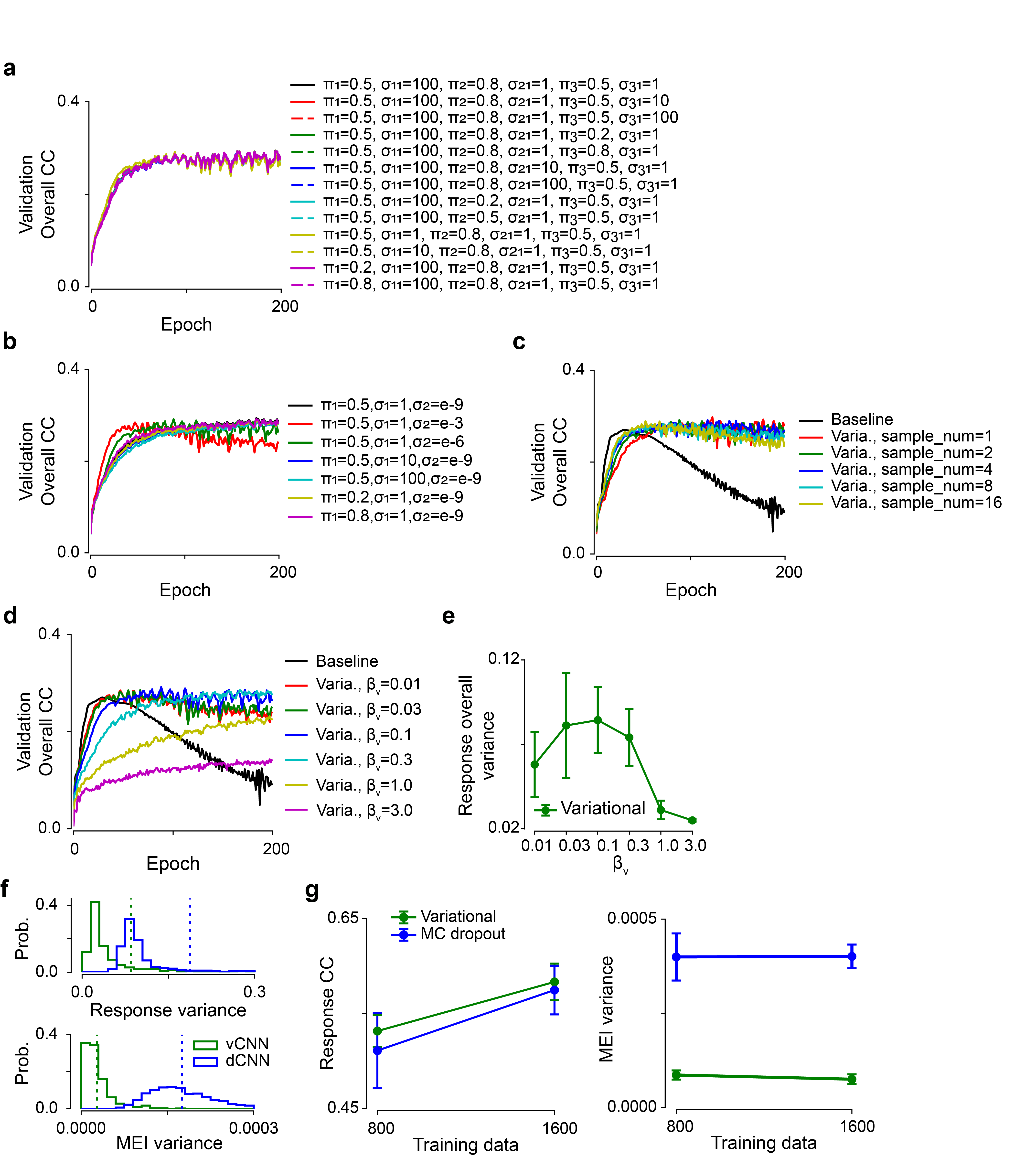
Figure 7: Neural prediction for first dataset. (a,b) Predictive performance (correlation coefficient, CC) based on validation data during training for variational models ($\beta_{v}=0.1$) with different prior distributions. All layers adopted the same $\sigma_{2}=\exp{(-6)}$ with different $\pi$ and $\sigma_{1}$ values (a), or with the same parameters of prior distribution (b). We picked $\pi=0.5,\sigma_{1}=1,\sigma_{2}=\exp{(-6)}$ for subsequent model training. (c) Predictive performance based on validation data during model training for different numbers of Monte Carlo sampling. We picked number=1 or 2 to save training time. (d) Model performance based on validation data during training for the baseline and variatonal models with different $\beta_{v}$ values. (e) Overall variance of predicted responses to test stimuli for different $\beta_{v}$ values. (f) Histogram of response variance (top) and MEI (RF) variance (bottom) for the variational and the MC dropout models. Dotted line represents the mean of histogram. (g) Model performance (left) based on test data and RF overall variance (right) for two probabilistic models with different amounts of training data. Error bars in (e) and (g) represent standard deviation of n=10 random seeds for each model.

5.2.2 Neural prediction for second dataset

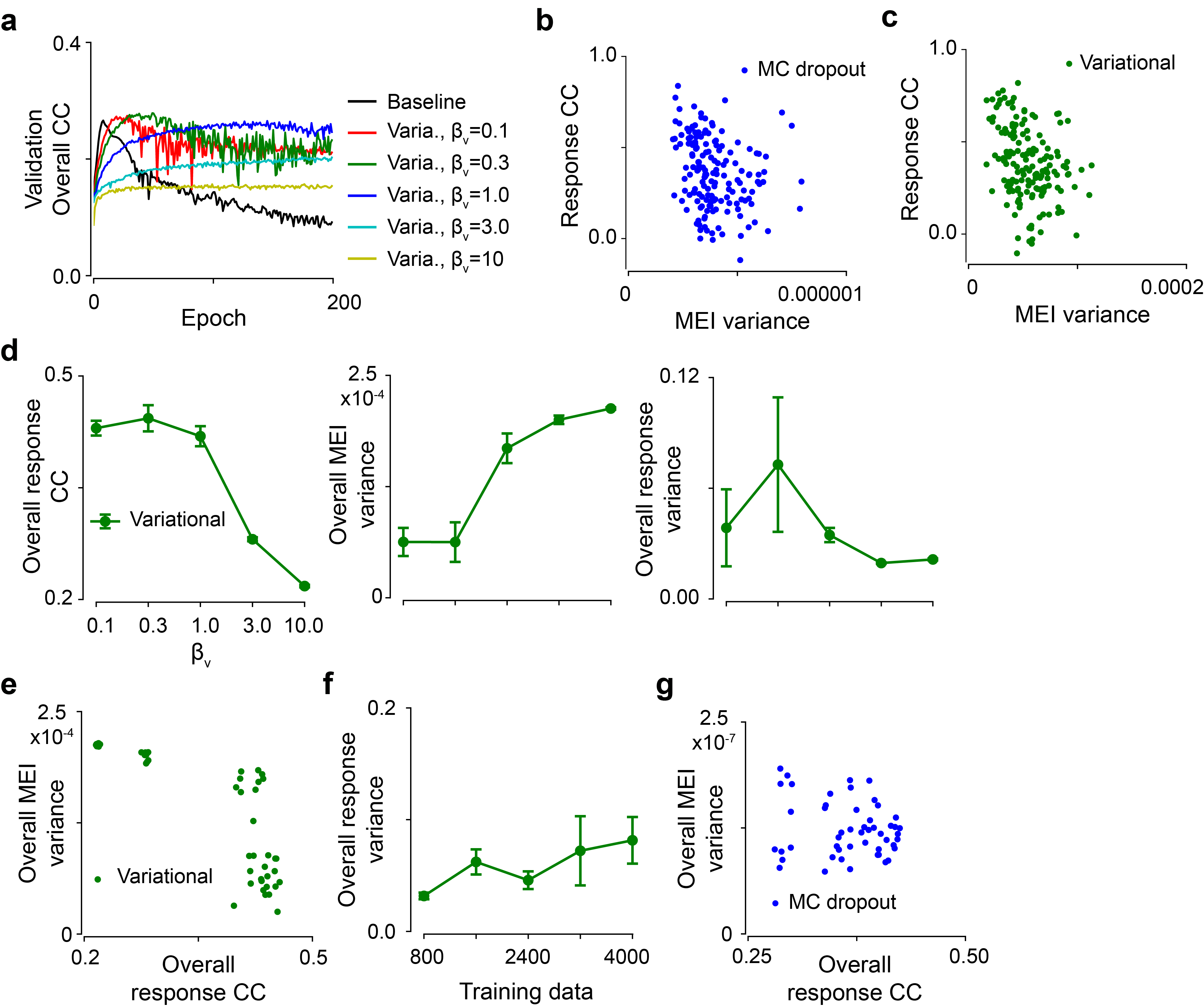
Figure 8: Neural prediction for second dataset. (a) Model performance based on validation data during training for the baseline and the variational models with different $\beta_{v}$ values. (b,c) Scatter plot of response CC and MEI (RF) variance for MC dropout (b) and variational (c) models for 10 seeds ($CC=-0.25,p=0.001$ and $CC=-0.34,p<0.0001$ for dropout and variational one, each dot representing one neuron at one random seed). (d) Predictive performance, overall RF variance and overall response variance for variational models with different $\beta_{v}$ values. (c) Predictive performance based on validation data during model training for different numbers of Monte Carlo sampling. We picked number=1 or 2 to save training time. (d) Model performance based on validation data during training for the baseline and the variational ones with different $\beta_{v}$ values. (e) Scatter plot for overall response CC and overall RF variance for the variational methods with different $\beta_{v}$ values (d) and at 10 seeds ($CC=-0.82,p<0.0001$). Each dot represents one model. (f) Overall response variance for different amounts of training data for the variational models (10 seeds per model). (g) Scatter plot for overall response CC and overall RF variance for the dropout model with different amounts of training data and at 10 seeds ($CC=-0.17,p=0.24$). Each dot represents one model. Error bars in (d) and (f) represent standard deviation of n=10 random seeds for each model.

5.2.3 Variance of predicted vs. recorded responses for second dataset

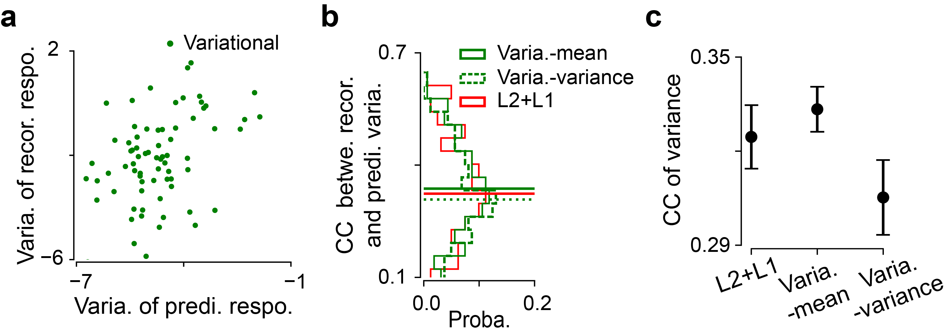
Figure 9: Variance of predicted vs. recorded responses for second dataset. Using the trained models, we tested whether the variance of predicted responses was related to the variance of recorded responses for each neuron. We first estimated the predicted response variance to a stimulus. For the L2+L1 model, as the mean of neural responses is proportional to the variance, we used the model output (a single predicted value) as a substitute. For the variational one, we either used the mean of predicted responses (multiple sampling times) as a substitute or calculated the response variance explicitly. (a) Scatter plot (axes in log scale) of predicted response variance (using response mean as a substitute) and recorded response variance for one neuron for a variational model. Each dot representing one stimulus. (b) Distribution of correlations between recorded and predicted response variance for all neurons for the L2+L1, variational-mean (using response mean as a substitute) and variational-variance (calculating response variance), at one random seed. Horizontal lines representing distribution means. (c) Mean correlations between two response variances (10 seeds per model). Note that variational-variance had lower correlation than the L2+L1. Error bars represent standard deviation of n=10 random seeds for each model. We computed the correlation using the predicted and recorded response variances of the test stimuli for each neuron ($CC=0.34,p=0.002$, Spearman correlation for an exemplary neuron; a). We found that the variational one using response mean as a substitute of variance had a slightly higher mean correlation across neurons compared to the L2+L1 ($p=0.0368$, two-sided permutation tests on 10 random seeds for 10,000 times; b,c).

5.2.4 Neural activation test with verified MEIs for second dataset

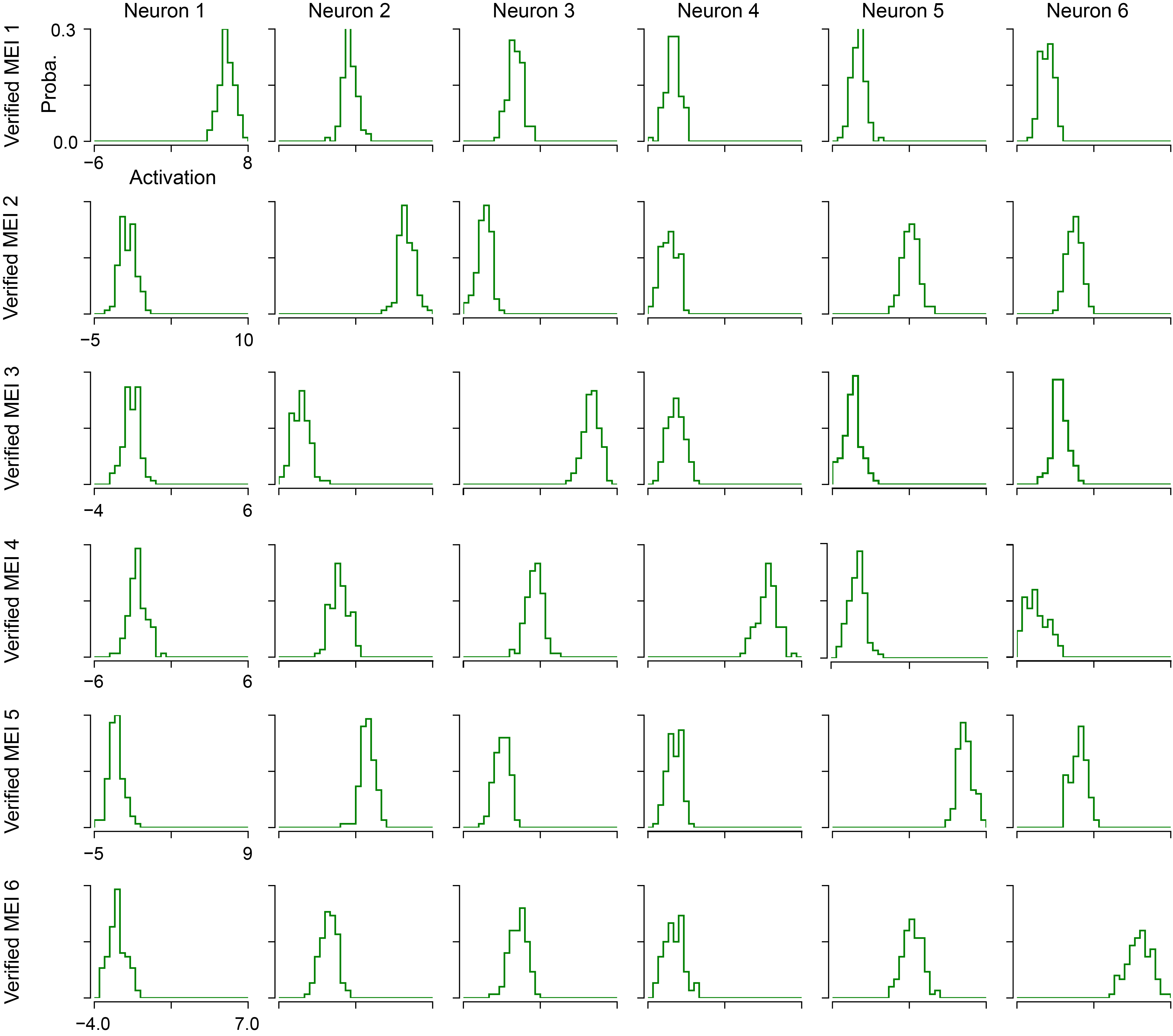
Figure 10: Neural activation test with verified MEIs for second dataset. Instead of performing closed-loop experiments to examine the effectiveness of our veriational model, we used the verified MEIs from previous study to compare the neuronal activities driven by different stimuli [Franke et al., 2021]. We plotted 1D histograms of activation of 6 exemplary cells (from left to right) driven by the verified MEIs (from top to bottom). Interestingly, each MEI from Franke et al. [2021] drove the corresponding neurons optimally.

References

- Abbott and Dayan [1999] Larry F Abbott and Peter Dayan. The effect of correlated variability on the accuracy of a population code. Neural computation, 11(1):91–101, 1999.
- Abdar et al. [2021] Moloud Abdar, Farhad Pourpanah, Sadiq Hussain, Dana Rezazadegan, Li Liu, Mohammad Ghavamzadeh, Paul Fieguth, Xiaochun Cao, Abbas Khosravi, U Rajendra Acharya, et al. A review of uncertainty quantification in deep learning: Techniques, applications and challenges. Information fusion, 76:243–297, 2021.
- Alemi et al. [2016] Alexander A Alemi, Ian Fischer, Joshua V Dillon, and Kevin Murphy. Deep variational information bottleneck. arXiv preprint arXiv:1612.00410, 2016.
- Antolík et al. [2016] Ján Antolík, Sonja B Hofer, James A Bednar, and Thomas D Mrsic-Flogel. Model constrained by visual hierarchy improves prediction of neural responses to natural scenes. PLoS computational biology, 12(6):e1004927, 2016.
- Averbeck et al. [2006] Bruno B Averbeck, Peter E Latham, and Alexandre Pouget. Neural correlations, population coding and computation. Nature reviews neuroscience, 7(5):358–366, 2006.
- Bashiri et al. [2021] Mohammad Bashiri, Edgar Walker, Konstantin-Klemens Lurz, Akshay Jagadish, Taliah Muhammad, Zhiwei Ding, Zhuokun Ding, Andreas Tolias, and Fabian Sinz. A flow-based latent state generative model of neural population responses to natural images. Advances in Neural Information Processing Systems, 34:15801–15815, 2021.
- Bashivan et al. [2019] Pouya Bashivan, Kohitij Kar, and James J DiCarlo. Neural population control via deep image synthesis. Science, 364(6439), 2019.
- Batty et al. [2016] Eleanor Batty, Josh Merel, Nora Brackbill, Alexander Heitman, Alexander Sher, Alan Litke, EJ Chichilnisky, and Liam Paninski. Multilayer recurrent network models of primate retinal ganglion cell responses. 2016.
- Blundell et al. [2015] Charles Blundell, Julien Cornebise, Koray Kavukcuoglu, and Daan Wierstra. Weight uncertainty in neural networks. arXiv preprint arXiv:1505.05424, 2015.
- Burgess et al. [2018] Christopher P Burgess, Irina Higgins, Arka Pal, Loic Matthey, Nick Watters, Guillaume Desjardins, and Alexander Lerchner. Understanding disentangling in -vae. arXiv preprint arXiv:1804.03599, 2018.
- Chiao and Masland [2003] Chuan-Chin Chiao and Richard H Masland. Contextual tuning of direction-selective retinal ganglion cells. Nature neuroscience, 6(12):1251–1252, 2003.
- Chichilnisky [2001] EJ Chichilnisky. A simple white noise analysis of neuronal light responses. Network: Computation in Neural Systems, 12(2):199–213, 2001.
- Cohen and Maunsell [2009] Marlene R Cohen and John HR Maunsell. Attention improves performance primarily by reducing interneuronal correlations. Nature neuroscience, 12(12):1594–1600, 2009.
- Cohen and Newsome [2008] Marlene R Cohen and William T Newsome. Context-dependent changes in functional circuitry in visual area mt. Neuron, 60(1):162–173, 2008.
- Cotton et al. [2020] Ronald James Cotton, Fabian Sinz, and Andreas Tolias. Factorized neural processes for neural processes: K-shot prediction of neural responses. Advances in Neural Information Processing Systems, 33:11368–11379, 2020.
- Da Silveira and Rieke [2021] Rava Azeredo Da Silveira and Fred Rieke. The geometry of information coding in correlated neural populations. arXiv preprint arXiv:2102.00772, 2021.
- Doiron et al. [2016] Brent Doiron, Ashok Litwin-Kumar, Robert Rosenbaum, Gabriel K Ocker, and Krešimir Josić. The mechanics of state-dependent neural correlations. Nature neuroscience, 19(3):383–393, 2016.
- Ecker et al. [2010] Alexander S Ecker, Philipp Berens, Georgios A Keliris, Matthias Bethge, Nikos K Logothetis, and Andreas S Tolias. Decorrelated neuronal firing in cortical microcircuits. science, 327(5965):584–587, 2010.
- Ecker et al. [2014] Alexander S Ecker, Philipp Berens, R James Cotton, Manivannan Subramaniyan, George H Denfield, Cathryn R Cadwell, Stelios M Smirnakis, Matthias Bethge, and Andreas S Tolias. State dependence of noise correlations in macaque primary visual cortex. Neuron, 82(1):235–248, 2014.
- Ecker et al. [2018] Alexander S Ecker, Fabian H Sinz, Emmanouil Froudarakis, Paul G Fahey, Santiago A Cadena, Edgar Y Walker, Erick Cobos, Jacob Reimer, Andreas S Tolias, and Matthias Bethge. A rotation-equivariant convolutional neural network model of primary visual cortex. arXiv preprint arXiv:1809.10504, 2018.
- Erhan et al. [2009] Dumitru Erhan, Yoshua Bengio, Aaron Courville, and Pascal Vincent. Visualizing higher-layer features of a deep network. University of Montreal, 1341(3):1, 2009.
- Faisal et al. [2008] A Aldo Faisal, Luc PJ Selen, and Daniel M Wolpert. Noise in the nervous system. Nature reviews neuroscience, 9(4):292–303, 2008.
- Field [1994] David J Field. What is the goal of sensory coding? Neural computation, 6(4):559–601, 1994.
- Fortuin et al. [2021] Vincent Fortuin, Adrià Garriga-Alonso, Sebastian W Ober, Florian Wenzel, Gunnar Rätsch, Richard E Turner, Mark van der Wilk, and Laurence Aitchison. Bayesian neural network priors revisited. arXiv preprint arXiv:2102.06571, 2021.
- Franke et al. [2021] Katrin Franke, Konstantin F Willeke, Kayla Ponder, Mario Galdamez, Taliah Muhammad, Saumil Patel, Emmanouil Froudarakis, Jacob Reimer, Fabian Sinz, and Andreas Tolias. Behavioral state tunes mouse vision to ethological features through pupil dilation. bioRxiv, 2021.
- Fu et al. [2023] Jiakun Fu, Suhas Shrinivasan, Kayla Ponder, Taliah Muhammad, Zhuokun Ding, Eric Wang, Zhiwei Ding, Dat T Tran, Paul G Fahey, Stelios Papadopoulos, et al. Pattern completion and disruption characterize contextual modulation in mouse visual cortex. bioRxiv, pages 2023–03, 2023.
- Gal and Ghahramani [2016] Yarin Gal and Zoubin Ghahramani. Dropout as a bayesian approximation: Representing model uncertainty in deep learning. In international conference on machine learning, pages 1050–1059. PMLR, 2016.
- Gawlikowski et al. [2023] Jakob Gawlikowski, Cedrique Rovile Njieutcheu Tassi, Mohsin Ali, Jongseok Lee, Matthias Humt, Jianxiang Feng, Anna Kruspe, Rudolph Triebel, Peter Jung, Ribana Roscher, et al. A survey of uncertainty in deep neural networks. Artificial Intelligence Review, 56(Suppl 1):1513–1589, 2023.
- Gerwinn et al. [2007] Sebastian Gerwinn, Matthias Bethge, Jakob H Macke, and Matthias Seeger. Bayesian inference for spiking neuron models with a sparsity prior. Advances in neural information processing systems, 20, 2007.
- Gerwinn et al. [2010] Sebastian Gerwinn, Jakob H Macke, and Matthias Bethge. Bayesian inference for generalized linear models for spiking neurons. Frontiers in computational neuroscience, 4:1299, 2010.
- Gneiting and Raftery [2007] Tilmann Gneiting and Adrian E Raftery. Strictly proper scoring rules, prediction, and estimation. Journal of the American statistical Association, 102(477):359–378, 2007.
- Goris et al. [2014] Robbe LT Goris, J Anthony Movshon, and Eero P Simoncelli. Partitioning neuronal variability. Nature neuroscience, 17(6):858–865, 2014.
- Güçlü and van Gerven [2015] Umut Güçlü and Marcel AJ van Gerven. Deep neural networks reveal a gradient in the complexity of neural representations across the ventral stream. Journal of Neuroscience, 35(27):10005–10014, 2015.
- Higgins et al. [2016] Irina Higgins, Loic Matthey, Arka Pal, Christopher Burgess, Xavier Glorot, Matthew Botvinick, Shakir Mohamed, and Alexander Lerchner. beta-vae: Learning basic visual concepts with a constrained variational framework. 2016.
- Hinton and Van Camp [1993] Geoffrey E Hinton and Drew Van Camp. Keeping the neural networks simple by minimizing the description length of the weights. In Proceedings of the sixth annual conference on Computational learning theory, pages 5–13, 1993.
- Hock et al. [1974] Howard S Hock, Gregory P Gordon, and Robert Whitehurst. Contextual relations: the influence of familiarity, physical plausibility, and belongingness. Perception & Psychophysics, 16:4–8, 1974.
- Hoefling et al. [2022] Larissa Hoefling, Klaudia P Szatko, Christian Behrens, Yongrong Qiu, David Alexander Klindt, Zachary Jessen, Gregory S Schwartz, Matthias Bethge, Philipp Berens, Katrin Franke, et al. A chromatic feature detector in the retina signals visual context changes. bioRxiv, 2022.
- Huang et al. [2021] Ziwei Huang, Yanli Ran, Jonathan Oesterle, Thomas Euler, and Philipp Berens. Estimating smooth and sparse neural receptive fields with a flexible spline basis. arXiv preprint arXiv:2108.07537, 2021.
- Hubel and Wiesel [1959] David H Hubel and Torsten N Wiesel. Receptive fields of single neurones in the cat’s striate cortex. The Journal of physiology, 148(3):574, 1959.
- Jaakkola and Jordan [2000] Tommi S Jaakkola and Michael I Jordan. Bayesian parameter estimation via variational methods. Statistics and Computing, 10(1):25–37, 2000.
- Karamanlis and Gollisch [2021] Dimokratis Karamanlis and Tim Gollisch. Nonlinear spatial integration underlies the diversity of retinal ganglion cell responses to natural images. Journal of Neuroscience, 41(15):3479–3498, 2021.
- Kingma and Welling [2013] Diederik P Kingma and Max Welling. Auto-encoding variational bayes. arXiv preprint arXiv:1312.6114, 2013.
- Klindt et al. [2017] David Klindt, Alexander S Ecker, Thomas Euler, and Matthias Bethge. Neural system identification for large populations separating “what” and “where”. In Advances in Neural Information Processing Systems, pages 3506–3516, 2017.
- Kohn et al. [2016] Adam Kohn, Ruben Coen-Cagli, Ingmar Kanitscheider, and Alexandre Pouget. Correlations and neuronal population information. Annual review of neuroscience, 39:237, 2016.
- Kuhn and Tucker [1951] Harold W Kuhn and Albert W Tucker. Nonlinear programming. In Proceedings of 2nd Berkeley Symposium, pages 481–492, 1951.
- Lakshminarayanan et al. [2017] Balaji Lakshminarayanan, Alexander Pritzel, and Charles Blundell. Simple and scalable predictive uncertainty estimation using deep ensembles. Advances in neural information processing systems, 30, 2017.
- Li et al. [2015] Yingzhen Li, José Miguel Hernández-Lobato, and Richard E Turner. Stochastic expectation propagation. Advances in neural information processing systems, 28, 2015.
- Lurz et al. [2021] Konstantin-Klemens Lurz, Mohammad Bashiri, Konstantin Willeke, Akshay K Jagadish, Eric Wang, Edgar Y Walker, Santiago A Cadena, Taliah Muhammad, Erick Cobos, Andreas S Tolias, et al. Generalization in data-driven models of primary visual cortex. BioRxiv, pages 2020–10, 2021.
- Mackay [1992] David John Cameron Mackay. Bayesian methods for adaptive models. California Institute of Technology, 1992.
- Matheson and Winkler [1976] James E Matheson and Robert L Winkler. Scoring rules for continuous probability distributions. Management science, 22(10):1087–1096, 1976.
- McIntosh et al. [2016] Lane McIntosh, Niru Maheswaranathan, Aran Nayebi, Surya Ganguli, and Stephen Baccus. Deep learning models of the retinal response to natural scenes. In Advances in neural information processing systems, pages 1369–1377, 2016.
- Mitchell et al. [2009] Jude F Mitchell, Kristy A Sundberg, and John H Reynolds. Spatial attention decorrelates intrinsic activity fluctuations in macaque area v4. Neuron, 63(6):879–888, 2009.
- Neal and Hinton [1998] Radford M Neal and Geoffrey E Hinton. A view of the em algorithm that justifies incremental, sparse, and other variants. In Learning in graphical models, pages 355–368. Springer, 1998.
- Olshausen and Millman [1999] Bruno Olshausen and K Millman. Learning sparse codes with a mixture-of-gaussians prior. Advances in neural information processing systems, 12, 1999.
- Olshausen and Field [1996] Bruno A Olshausen and David J Field. Emergence of simple-cell receptive field properties by learning a sparse code for natural images. Nature, 381(6583):607–609, 1996.
- Park and Pillow [2011] Il Memming Park and Jonathan Pillow. Bayesian spike-triggered covariance analysis. Advances in neural information processing systems, 24, 2011.
- Perkel et al. [1967] Donald H Perkel, George L Gerstein, and George P Moore. Neuronal spike trains and stochastic point processes: Ii. simultaneous spike trains. Biophysical journal, 7(4):419–440, 1967.
- Pillow et al. [2008] Jonathan W Pillow, Jonathon Shlens, Liam Paninski, Alexander Sher, Alan M Litke, EJ Chichilnisky, and Eero P Simoncelli. Spatio-temporal correlations and visual signalling in a complete neuronal population. Nature, 454(7207):995–999, 2008.
- Ponce et al. [2019] Carlos R Ponce, Will Xiao, Peter F Schade, Till S Hartmann, Gabriel Kreiman, and Margaret S Livingstone. Evolving images for visual neurons using a deep generative network reveals coding principles and neuronal preferences. Cell, 177(4):999–1009, 2019.
- Posch and Pilz [2020] Konstantin Posch and Juergen Pilz. Correlated parameters to accurately measure uncertainty in deep neural networks. IEEE Transactions on Neural Networks and Learning Systems, 32(3):1037–1051, 2020.
- Qiu et al. [2021] Yongrong Qiu, Zhijian Zhao, David Klindt, Magdalena Kautzky, Klaudia P Szatko, Frank Schaeffel, Katharina Rifai, Katrin Franke, Laura Busse, and Thomas Euler. Natural environment statistics in the upper and lower visual field are reflected in mouse retinal specializations. Current Biology, 31(15):3233–3247, 2021.
- Qiu et al. [2023] Yongrong Qiu, David A Klindt, Klaudia P Szatko, Dominic Gonschorek, Larissa Hoefling, Timm Schubert, Laura Busse, Matthias Bethge, and Thomas Euler. Efficient coding of natural scenes improves neural system identification. PLOS Computational Biology, 19(4):e1011037, 2023.
- Richards et al. [2019] Blake A Richards, Timothy P Lillicrap, Philippe Beaudoin, Yoshua Bengio, Rafal Bogacz, Amelia Christensen, Claudia Clopath, Rui Ponte Costa, Archy de Berker, Surya Ganguli, et al. A deep learning framework for neuroscience. Nature neuroscience, 22(11):1761–1770, 2019.
- Ritter et al. [2018] Hippolyt Ritter, Aleksandar Botev, and David Barber. A scalable laplace approximation for neural networks. In 6th International Conference on Learning Representations, ICLR 2018-Conference Track Proceedings, volume 6. International Conference on Representation Learning, 2018.
- Rust and Movshon [2005] Nicole C Rust and J Anthony Movshon. In praise of artifice. Nature neuroscience, 8(12):1647–1650, 2005.
- Saxe et al. [2021] Andrew Saxe, Stephanie Nelli, and Christopher Summerfield. If deep learning is the answer, what is the question? Nature Reviews Neuroscience, 22(1):55–67, 2021.
- Srivastava et al. [2014] Nitish Srivastava, Geoffrey Hinton, Alex Krizhevsky, Ilya Sutskever, and Ruslan Salakhutdinov. Dropout: a simple way to prevent neural networks from overfitting. The journal of machine learning research, 15(1):1929–1958, 2014.
- Stein [1967] Richard B Stein. Some models of neuronal variability. Biophysical journal, 7(1):37–68, 1967.
- Stevenson et al. [2008] Ian H Stevenson, James M Rebesco, Nicholas G Hatsopoulos, Zach Haga, Lee E Miller, and Konrad P Kording. Bayesian inference of functional connectivity and network structure from spikes. IEEE Transactions on Neural Systems and Rehabilitation Engineering, 17(3):203–213, 2008.
- Tishby et al. [2000] Naftali Tishby, Fernando C Pereira, and William Bialek. The information bottleneck method. arXiv preprint physics/0004057, 2000.
- Tong et al. [2023] Rudi Tong, Ronan da Silva, Dongyan Lin, Arna Ghosh, James Wilsenach, Erica Cianfarano, Pouya Bashivan, Blake Richards, and Stuart Trenholm. The feature landscape of visual cortex. bioRxiv, pages 2023–11, 2023.
- Walker et al. [2019] Edgar Y Walker, Fabian H Sinz, Erick Cobos, Taliah Muhammad, Emmanouil Froudarakis, Paul G Fahey, Alexander S Ecker, Jacob Reimer, Xaq Pitkow, and Andreas S Tolias. Inception loops discover what excites neurons most using deep predictive models. Nature neuroscience, 22(12):2060–2065, 2019.
- Wu et al. [2006] Michael C-K Wu, Stephen V David, and Jack L Gallant. Complete functional characterization of sensory neurons by system identification. Annu. Rev. Neurosci., 29:477–505, 2006.
- Yamins et al. [2014] Daniel LK Yamins, Ha Hong, Charles F Cadieu, Ethan A Solomon, Darren Seibert, and James J DiCarlo. Performance-optimized hierarchical models predict neural responses in higher visual cortex. Proceedings of the National Academy of Sciences, 111(23):8619–8624, 2014.
- Yu et al. [2008] Byron M Yu, John P Cunningham, Gopal Santhanam, Stephen Ryu, Krishna V Shenoy, and Maneesh Sahani. Gaussian-process factor analysis for low-dimensional single-trial analysis of neural population activity. Advances in neural information processing systems, 21, 2008.