Augmented Negative Sampling for Collaborative Filtering

Abstract.

Negative sampling is essential for implicit-feedback-based collaborative filtering, which is used to constitute negative signals from massive unlabeled data to guide supervised learning. The state-of-the-art idea is to utilize hard negative samples that carry more useful information to form a better decision boundary. To balance efficiency and effectiveness, the vast majority of existing methods follow the two-pass approach, in which the first pass samples a fixed number of unobserved items by a simple static distribution and then the second pass selects the final negative items using a more sophisticated negative sampling strategy. However, selecting negative samples from the original items in a dataset is inherently restricted due to the limited available choices, and thus may not be able to contrast positive samples well. In this paper, we confirm this observation via carefully designed experiments and introduce two major limitations of existing solutions: ambiguous trap and information discrimination.

Our response to such limitations is to introduce “augmented” negative samples that may not exist in the original dataset. This direction renders a substantial technical challenge because constructing unconstrained negative samples may introduce excessive noise that eventually distorts the decision boundary. To this end, we introduce a novel generic augmented negative sampling (ANS) paradigm and provide a concrete instantiation. First, we disentangle hard and easy factors of negative items. Next, we generate new candidate negative samples by augmenting only the easy factors in a regulated manner: the direction and magnitude of the augmentation are carefully calibrated. Finally, we design an advanced negative sampling strategy to identify the final augmented negative samples, which considers not only the score function used in existing methods but also a new metric called augmentation gain. Extensive experiments on real-world datasets demonstrate that our method significantly outperforms state-of-the-art baselines. Our code is publicly available at https://github.com/Asa9aoTK/ANS-Recbole.

1. Introduction

Collaborative filtering (CF), as an important paradigm of recommender systems, leverages observed user-item interactions to model users’ potential preferences (He et al., 2020, 2017; Wang et al., 2019). In real-world scenarios, such interactions are normally in the form of implicit feedback (e.g., clicks or purchases), instead of explicit ratings (Wang et al., 2021).Each observed interaction is normally considered a positive sample. As for negative samples, existing methods usually randomly select some uninteracted items. Then a CF model is optimized to give positive samples higher scores than negative ones via, for example, the Bayesian personalized ranking (BPR) loss function (Rendle et al., 2009), where a score function (e.g., inner product) is used to measure the similarity between a user and an item.

Recent studies have shown that negative samples have a great impact on model performance (Zhuo et al., 2022; Mao et al., 2021; Zhang et al., 2013). As the state of the art, hard negative sampling strategies whose general idea is to oversample high-score negative items have exhibited promising performance (Zhang et al., 2013; Ding et al., 2019, 2020; Zhu et al., 2022; Chen et al., 2022). While selecting a negative item with a high score makes it harder for a model to classify a user, it has the potential to bring more useful information and greater gradients, which are beneficial to model training (Rendle and Freudenthaler, 2014; Chen et al., 2022). Ideally, one would calculate the scores of all uninteracted items to identify the best negative samples. However, its time complexity is prohibitive. To balance efficiency and effectiveness, the two-pass approach has been widely adopted (Bai et al., 2017; Zhang et al., 2013; Ding et al., 2020; Zhu et al., 2022; Huang et al., 2021). The first pass samples a fixed number of unobserved items by a static distribution, and the second pass then selects the final negative items with a more sophisticated negative sampling method.

Despite the significant progress made by hard negative sampling, selecting negative samples from the original items in a dataset is inherently restricted due to the limited available choices. Such original items may not be able to contrast positive samples well. Indeed, we design a set of intuitive experiments to show that existing works suffer from two major drawbacks. (1) Ambiguous trap. Since the vast majority of unobserved items have very low scores (i.e., they are easy negative samples), randomly sampling a small number of candidate negative items in the first pass is difficult to include useful hard negative samples, which, in turn, substantially limits the efficacy of the second pass. (2) Information discrimination. In the second pass, most existing studies overly focus on high-score negative items and largely neglect low-score negative items. We empirically show that such low-score negative items also contain critical, unique information that leads to better model performance.

Our response to such drawbacks is to introduce “augmented” negative samples (i.e., synthetic items) that are more similar to positive items while still being negative. While data augmentation techniques have been proposed in other domains (Kalantidis et al., 2020; Yu et al., 2022; Wu et al., 2021; Xia et al., 2021), it is technically challenging to apply similar ideas to negative sampling for collaborative filtering. This is because all of them fail to carefully regulate and quantify the augmentation needed to approximate positive items while not introducing excessive noise or still being negative.

To this end, we present a novel generic augmented negative sampling (ANS) paradigm and then provide a concrete instantiation. Our insight is that it is imperative to understand a negative item’s hardness from a more fine-granular perspective. We propose to disentangle an item’s embedding into hard and easy factors (i.e., a set of dimensions of the embedding vector), where hardness is defined by whether a negative item has similar values to the corresponding user in the given factor. This definition is in line with the definition of hardness in hard negative sampling. Here the key technical challenge originates from the lack of supervision signals. Consequently, we propose two learning tasks that combine contrastive learning (CL) (Zheng et al., 2022) and disentanglement methods (Han et al., 2022) to guarantee the credibility of the disentanglement. Since our goal is to create synthetic negative items similar to positive items, we keep the hard factor of a negative item unchanged and focus on augmenting the easy factor by controlling the direction and magnitude of added noise. The augmentation mechanism needs to be carefully designed so that the augmented item will become more similar to the corresponding positive item, but will not cross the decision boundary. Furthermore, we introduce a new metric called augmentation gain to measure the difference between the scores before and after the augmentation. Our sampling strategy is guided by augmentation gain, which gives low-score items with higher augmentation gain a larger probability of being sampled. In this way, we can effectively mitigate information discrimination, leading to better performance. We summarize our main contributions as follows:

• We design a set of intuitive experiments to reveal two notable limitations of existing hard negative sampling methods, namely ambiguous trap and information discrimination.

• To the best of our knowledge, we are the first to propose to generate negative samples from a fine-granular perspective to improve implicit CF. In particular, we propose a new direction of generating regulated augmentation to address the unique challenges of CF.

• We propose a general paradigm called augmented negative sampling (ANS) that consists of three steps, including disentanglement, augmentation, and sampling. We also present a concrete implementation of ANS, which is not only performant but also efficient.

• We conduct extensive experiments on five real-world datasets to demonstrate that ANS can achieve significant improvements over representative state-of-the-art negative sampling methods.

2. Related Work

2.1. Model-Agnostic Negative Sampling

A common type of negative sampling strategy selects negative samples based on a pre-determined static distribution (Chen et al., 2017; Wu et al., 2019; Yang et al., 2020). Such a strategy is normally efficient since it does not need to be adjusted in the model training process. Random negative sampling (RNS) (Rendle et al., 2009; Wang et al., 2019; Yu et al., 2022; Chen et al., 2020b) is a simple and representative model-agnostic sampling strategy, which selects negative samples from unobserved items according to a uniform distribution. However, the uniform distribution is difficult to guarantee the quality of negative samples. Inspired by the word-frequency-based distribution (Grover and Leskovec, 2016) and node-degree-based distribution (Mikolov et al., 2013) in other domains, an item-popularity-based distribution (Chen et al., 2017; Bengio and Senécal, 2008) has been introduced. Under this distribution, popular items are more likely to be sampled as negative items, which helps to mitigate the widespread popularity bias issue in recommender systems (Chen et al., 2020a). Although this kind of strategy is generally efficient, the pre-determined distributions are not customized for the underlying models and not adaptively adjusted during the training process. As a result, their performance is often sub-optimal.

2.2. Model-Aware Negative Sampling

These strategies take into consideration some information of the underlying model, denoted by $f$, to guide the sampling process. Given $f$, the probability of sampling an item $i$ is defined as $p(i\mid f)\propto g(f,\mathbf{e}_{i})$, where $g(\cdot,\cdot)$ is a sampling function, and $\mathbf{e}_{i}$ denotes the embedding of $i$. Existing studies focus on choosing different $f$ and/or designing a proper $g(\cdot,\cdot)$ to achieve better performance. The most representative work is hard negative sampling, which defines $g(\cdot,\cdot)$ as a score function. It assigns higher sampling probabilities to the negative items with larger prediction scores (Ding et al., 2019, 2020; Huang et al., 2021; Rendle and Freudenthaler, 2014; Zhang et al., 2013; Zhu et al., 2022). For example, DNS (Zhang et al., 2013) assumes that the high-score items should be more likely to be selected, and thus chooses $g(\cdot,\cdot)$ to be the inner product and $f$ to be user representations. With the goal of mitigating false negative samples, SRNS (Ding et al., 2020) further incorporates the information about the last few epochs into $f$ and designs $g(\cdot,\cdot)$ to give false negative samples lower scores. IRGAN (Wang et al., 2017) integrates a generative adversarial network into $g(\cdot,\cdot)$ to determine the probabilities of negative samples through the min-max game. ReinforcedNS (Ding et al., 2019) use reinforcement learning into $g(\cdot,\cdot)$.

With well-designed $f$ and $g(\cdot,\cdot)$, we can generally achieve better performance. However, selecting suitable negative items need to compute $g(\cdot,\cdot)$ for all unobserved items, which is extremely time-consuming and prohibitively expensive. Take DNS as an example. Calculating the probability of sampling an item is equivalent to performing softmax on all unobserved samples, which is unacceptable in real-world applications (Chen et al., 2022; Wang et al., 2017; Park and Chang, 2019). As a result, most model-aware sampling strategies adopt the two-pass approach or its variants. In this case, $g(\cdot,\cdot)$ is only applied to a small number of candidates sampled in the first pass. While such two-pass-based negative sampling strategies have been the mainstream methods, they exhibit two notable limitations, namely ambiguous trap and information discrimination, which motivates us to propose an augmented negative sampling paradigm. In the next section, we will explain these limitations via a set of intuitive experiments.

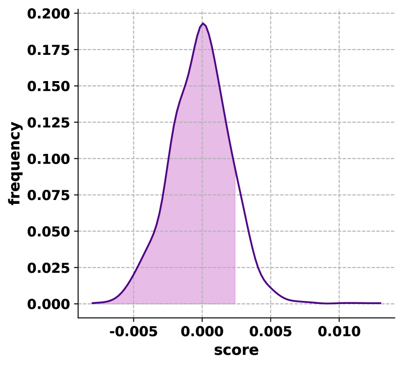
(a) Epoch 0

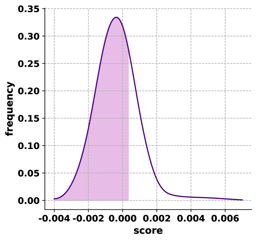
(b) Epoch 30

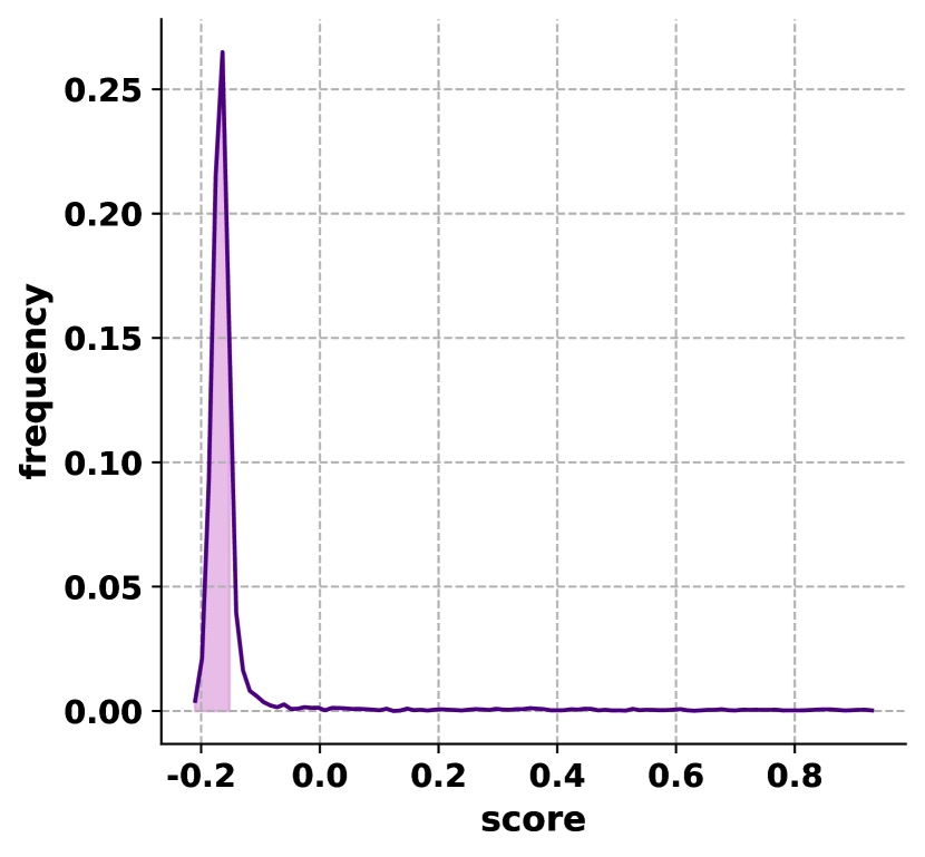
(c) Epoch 50

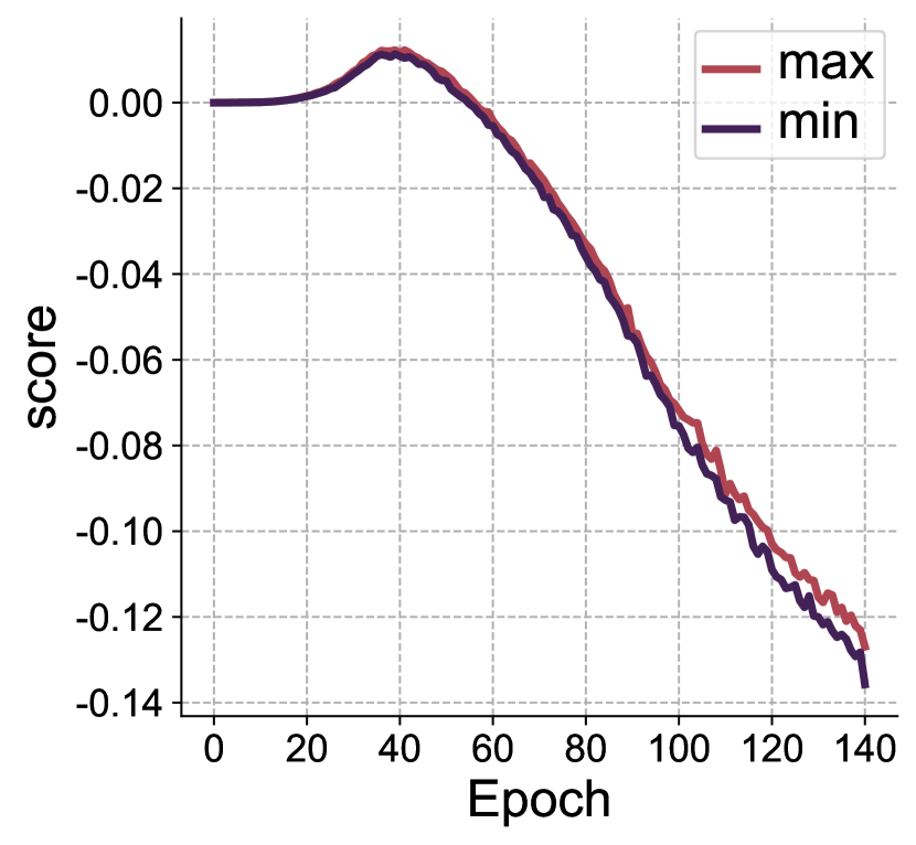
(d) Overall score

Figure 1. Experimental results to demonstrate the phenomenon of ambiguous trap in DNS.

3. Limitations of the Two-Pass Approach

In this section, we first formulate the problem of implicit CF and then explain ambiguous trap and information discrimination via intuitive experiments. We consider the Last.fm and Amazon-Baby datasets in experiments. A comprehensive description of the data is provided in Section 5.

3.1. Implicit CF

We denote the set of historical interactions by $\mathcal{O}^{+}=\{(u,i^{+})\mid u\in\mathcal{U},i^{+}\in\mathcal{I}\}$, where $\mathcal{U}$ and $\mathcal{I}$ are the set of users and the set of items, respectively. The most common implicit CF paradigm is to learn user and item representations ($\mathbf{e}_{u}$ and $\mathbf{e}_{i}$) from the historical interactions and then predict the scores of unobserved items to recommend the top-K items. The BPR loss function is widely used to optimize the model:

(1) $$\mathcal{L}_{\mathrm{BPR}}=\sum_{\begin{subarray}{c}(u,i^{+})\in\mathcal{O}^{+}\\ \end{subarray}}-\ln[\sigma(s(\mathbf{e}_{u},\mathbf{e}_{i^{+}})-s(\mathbf{e}_{u},\mathbf{e}_{i^{-}}))],$$

where $\sigma(\cdot)$ is the sigmoid function, and $s(\cdot,\cdot)$ is a score function (e.g., the inner product) that measures the similarity between the user and item representations. Here $i^{-}$ is a negative sample selected by a sampling strategy. Our goal is to design a negative sampling strategy that is generic to different CF models. Following previous studies (Chen et al., 2022; Rendle et al., 2009; Wang et al., 2017), without loss of generality, we consider matrix factorization with Bayesian personalized ranking (MF-BPR) (Rendle et al., 2009) as the basic CF model to illustrate ANS.

3.2. Ambiguous Trap

We choose DNS (Zhang et al., 2013), which is the most representative hard negative sampling method, to train an MF-BPR model on the Last.fm dataset and calculate the scores of unobserved user-item pairs in different training periods. Figure 1(a), 1(b), 1(c) demonstrates the frequency distributions of the scores at different epochs. The lowest 80% of the scores are emphasized by the pink shade. We can observe that as training progresses, more and more scores are concentrated in the low-score region, meaning that the vast majority of unobserved items are easy negative samples. Recall that the first pass samples a fixed number of negative items by a uniform distribution. Randomly sampling a small number of negative items in the first pass is difficult to include useful hard negative samples, which, in turn, substantially limits the efficacy of the second pass. We call this phenomenon ambiguous trap.

To further demonstrate the existence of ambiguous trap, in Figure 1(d), we plot the min-max normalizing maximum and minimum scores of the sampled negative items in the first pass on the Last.fm dataset. It can be seen that the difference between the maximum score and the minimum score is consistently small, suggesting that randomly sampling a small number of negative items makes the hardness of the negative samples obtained from DNS far from ideal. Note that a straightforward attempt to mitigate ambiguous trap is to substantially increase the sample size in the first pass. However, it is inevitably at the cost of substantial time and space overhead (Chen et al., 2022). Inspired by contrastive learning (Yu et al., 2022; Wu et al., 2021; Kalantidis et al., 2020), we propose to augment the sampled negative items to increase their hardness.

3.3. Information Discrimination

In the second pass, most existing studies overly focus on high-score negative items and largely neglect low-score negative items, which also contain critical, unique information to improve model performance. Overemphasizing high-score items as negative samples may result in worse model performance. Several studies (Chen et al., 2022; Shi et al., 2023) have made efforts to assign lower sampling probabilities to low-score items using algorithms like softmax and its derivatives. However, selecting those significantly lower-score items in comparison to others, remains a challenge. We call this behavior information discrimination. To verify the existence of information discrimination, we introduce a new measure named Pairwise Exclusive-hit Ratio (PER) (Kang et al., 2022) to CF, which is used to compare the difference between the information learned by two different methods. More specifically, $\operatorname{PER}(x,y)$ quantifies the information captured by the method $x$ but not by $y$ via

(2) $$\operatorname{PER}(x,y)=\frac{\left|\mathcal{H}_{x}-\mathcal{H}_{y}\right|}{\left|\mathcal{H}_{x}\right|},$$

where $\mathcal{H}_{x}$ denotes the set of test interactions correctly predicted by the method $x$. Next, we choose two representative negative sampling methods, RNS (Ding et al., 2019) and DNS (Zhang et al., 2013) to train MF-BPR models and calculate the PER between them. Recall that DNS is more likely to select high-score negative items while RNS uniformly randomly selects negative items irrespective of their scores. The obtained results are depicted in Figure 2 (excluding HNS data for the current analysis). We can observe that: (1) the DNS strategy can indeed learn more information, confirming the benefits of leveraging hard negative samples to form a tighter decision boundary. (2) The values of $\operatorname{PER}(\textrm{RNS},\textrm{DNS})$ on two datasets (0.2 and 0.33) indicate that even the simple RNS strategy can still learn rich information that is not learned by DNS. In other words, the easy negative items overlooked by DNS are still valuable for CF. Such an information discrimination problem inspires us to understand a negative item’s hardness from a more fine-granular perspective in order to extract more useful information.

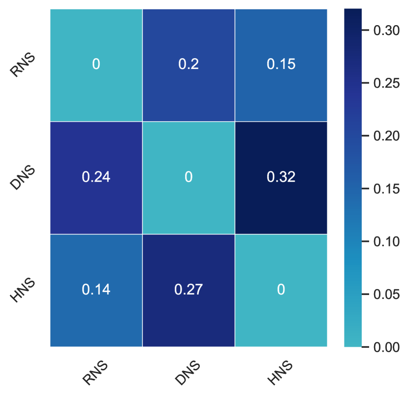
(a) Last.fm

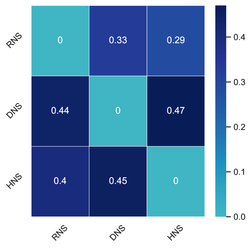
(b) Amazon-Beauty

Figure 2. PER values of different pairs of negative sampling methods.

4. Methodology

Driven by the aforementioned limitations, we propose a novel generic augmented negative sampling (ANS) paradigm, which consists of three major steps: disentanglement, augmentation, and sampling. The disentanglement step learns an item’s hard and easy factors; the augmentation step adds regulated noise to the easy factor so as to increase the item’s hardness; the sampling strategy selects the final negative samples based on a new metric we propose. The workflow of ANS is illustrated in Figure 3. Note that these steps can be implemented by different methods and thus the overall paradigm is generic. We present a possible instantiation in the following sections.

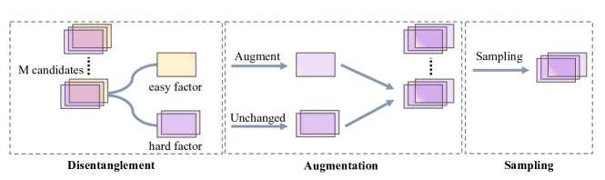
Figure 3. The workflow of augmented negative sampling (ANS) paradigm.

4.1. Disentanglement

To understand a negative item’s hardness from a more fine-granular perspective, we propose to disentangle its embedding into hard and easy factors (i.e., a set of dimensions of the embedding vector), where hardness is defined by whether a negative item has similar values to the corresponding user in the given factor. Similarly, we follow the two-pass approach to first randomly sample $M$ ($M\ll\left|\mathcal{I}\right|$) items from the unobserved items to form a candidate negative set $\mathcal{E}$. We design a gating module to identify which dimensions of a negative item $\mathbf{e}_{n}\in\mathbb{R}^{d}$ in $\mathcal{E}$ are hard with respect to user $\mathbf{e}_{u}\in\mathbb{R}^{d}$ via

(3) $$gate_{hard}=\sigma\left(\mathbf{W}_{item}\mathbf{e}_{n}\odot\mathbf{W}_{user}\mathbf{e}_{u}\right),$$

where $gate_{hard}\in\mathbb{R}^{d}$ gives the weights of different dimensions. The sigmoid function $\sigma(\cdot)$ maps the values to $(0,1)$. $\mathbf{W}_{item}\in\mathbb{R}^{d\times d}$ and $\mathbf{W}_{user}\in\mathbb{R}^{d\times d}$ are linear transformations used to ensure that the user and item embeddings are in the common latent space (Mao et al., 2021). $\odot$ is the element-wise product, which measures the similarity between $\mathbf{e}_{i}$ and $\mathbf{e}_{u}$ in each dimension (Wang et al., 2019). After obtaining the weights $gate_{hard}$, we adopt the element-wise product to extract the hard factor $\mathbf{e}_{n}^{hard}$. The easy factor $\mathbf{e}_{n}^{easy}$ is then calculated via element-wise subtraction (Han et al., 2022).

(4) $$\begin{split}\begin{aligned} \mathbf{e}_{n}^{hard}&=\mathbf{e}_{n}\odot gate_{hard},\\ \mathbf{e}_{n}^{easy}&=\mathbf{e}_{n}-\mathbf{e}_{n}^{hard}.\end{aligned}\end{split}$$

Due to the lack of ground truth for hard and easy factors, it is inherently difficult to guarantee the credibility of the disentanglement. Inspired by its superiority in unsupervised scenarios (Zheng et al., 2022; Khosla et al., 2020), we propose to adopt contrastive learning to guide the disentanglement. By definition, the hard factor of a negative item should be more similar to the user, while the easy factor should be the opposite. Therefore, given a score function $s(\cdot,\cdot)$ to calculate the similarity between a pair, we design a contrastive loss $\mathcal{L}_{c}$ as

(5) $$\begin{split}\begin{aligned} \mathcal{L}_{c}=\sum_{{e}_{n}\in\mathcal{E}}s(\mathbf{e}_{u},\mathbf{e}_{n}^{easy})-s(\mathbf{e}_{u},\mathbf{e}_{n}^{hard}).\end{aligned}\end{split}$$

However, optimizing only $\mathcal{L}_{c}$ may lead to a trivial solution: including all dimensions as the hard factor. Therefore, we introduce another loss with the auxiliary information from positive items. We adopt a similar operation with the same weights $gate_{hard}$ to obtain the corresponding positive item factor $\mathbf{e}_{p}^{\prime}$ and $\mathbf{e}_{p}^{\prime\prime}$:

(6) $$\begin{split}\begin{aligned} \mathbf{e}_{p}^{\prime}&=\mathbf{e}_{p}\odot gate_{hard},\\ \mathbf{e}_{p}^{\prime\prime}&=\mathbf{e}_{p}-\mathbf{e}_{p}^{\prime}.\end{aligned}\end{split}$$

This is particularly important as $\mathbf{e}_{n}^{easy}$ may emphasize the first 48 dimensions while $\mathbf{e}_{n}^{hard}$ may emphasize the last 14. In order to ensure coherence in subsequent operations, it is imperative to maintain the correspondence of dimensions. For ease of understanding, reader can directly regard them as positive samples. Intuitively, $\mathbf{e}_{n}^{hard}$ should be more similar to positive since it is difficult for users to discern it as a negative sample (both have a high similarity to the user). However, this signal is not entirely reliable, as it may not accurately reflect a user’s level of interest. Therefore, instead of relying on a stringent constraint like Equation 5, we introduce another disentanglement loss $\mathcal{L}_{d}$ as

(7) $$\begin{split}\begin{aligned} \mathcal{L}_{d}=\sum_{{e}_{n}\in\mathcal{E}}\left\|\mathbf{e}_{p}^{\prime}-\mathbf{e}_{n}^{hard}\right\|^{2}+s(\mathbf{e}_{p}^{\prime\prime},\mathbf{e}_{n}^{easy}),\end{aligned}\end{split}$$

where the Euclidean distance is used to measure the similarity between $\mathbf{e}_{p}^{\prime}$ and $\mathbf{e}_{n}^{hard}$ while the score function is used to measure the similarity between $\mathbf{e}_{p}^{easy}$ and $\mathbf{e}_{n}^{\prime\prime}$. This is because we want to leverage only reliable hardness while we can be more lenient with the easy part.

4.2. Augmentation

Next, we propose an augmentation module to create synthetic negative items which are more similar to the corresponding positive items. After the disentanglement step, we have obtained the hard and easy factors of a negative item, where the hard factor contains more useful information for model training. Therefore, our goal is to augment the easy factor to improve model performance. However, existing augmentation techniques fail to carefully regulate and quantify the augmentation needed to approximate positive items while still being negative. To this end, we propose to regulate the augmentation from two different aspects:

Direction: Intuitively, the direction of the augmentation on a negative item should be towards the corresponding positive item. Therefore, we first calculate the difference $\mathbf{e}_{dif}$ between the factor of the positive item $\mathbf{e}_{p}^{\prime\prime}$ and the easy factor of the negative item $\mathbf{e}_{n}^{easy}$:

(8) $$\begin{split}\begin{aligned} \mathbf{e}_{dif}&=\mathbf{e}_{p}^{\prime\prime}-\mathbf{e}_{n}^{easy}.\end{aligned}\end{split}$$

A first attempt is to directly make $\mathbf{e}_{dif}$ as the direction of the augmentation. This design is less desirable because (1) it introduces too much positive information, which may turn the augmented negative item into positive. (2) It contains too much prior information (i.e., the easy factor is identical to that of the positive item), which can lead to the model collapse problem (Srivastava et al., 2017; Thanh-Tung and Tran, 2020). Inspired by (Yu et al., 2022), we carefully smooth the direction of augmentation by extracting the quadrant information $\mathbf{e}_{dir}$ of $\mathbf{e}_{dif}$ with the sign function $sgn(\cdot)$:

(9) $$\begin{split}\begin{aligned} \mathbf{e}_{dir}&=sgn(\mathbf{e}_{dif}).\end{aligned}\end{split}$$

The direction $\mathbf{e}_{dir}\in\mathbb{R}^{d}$ effectively compresses the embedding augmentation space into a quadrant space, which provides essential direction information without having the aforementioned issues.

Magnitude: Magnitude determines the strength of augmentation. Several studies (He et al., 2018) have shown that when the perturbation to the embedding is overly large, it will dramatically change its original semantics. Therefore, we need to carefully calibrate the magnitude of the augmentation. We design a two-step approach to generate a regulated magnitude $\Delta\in\mathbb{R}^{d}$. We first consider the distribution of $\Delta$. As $\Delta$ is a noise embedding, we adopt a uniform distribution on the interval $[0,0.1]$. The uniform distribution introduces a certain amount of randomness, which is beneficial to improve the robustness of the model. Second, we restrict $\Delta$ to be smaller than a margin. Instead of using a static scalar (Mao et al., 2021), we dynamically set the margin by calculating the similarity between the hard factors of the negative and corresponding positive items. The intuition is that a higher similarity between the hard factors suggests that the negative item already contains much useful information, and thus we should augment it with a smaller magnitude. Finally, the regulated magnitude $\Delta$ is calculated via

(10) $$\begin{split}\begin{aligned} \|\Delta\|&\leq\sigma\left(\frac{1}{\mathbf{W}\left(\mathbf{e}_{n}^{hard}\odot\mathbf{e}_{p}^{\prime}\right)}\right),\end{aligned}\end{split}$$

where the element-wise product $\odot$ is used to calculate the similarity between $\mathbf{e}_{n}^{hard}$ and $\mathbf{e}_{p}^{\prime}$. The transformation matrix $\mathbf{W}\in\mathbb{R}^{1\times d}$ is used to map the similarity vector to a scalar. The sigmoid function $\sigma(\cdot)$ helps remove the sign information to avoid interfering with the learned direction $\mathbf{e}_{dir}$. After carefully determining the direction and magnitude, we can generate the augmented version $\mathbf{e}_{n}^{aug}$ of the negative item $\mathbf{e}_{n}$ as follows:

(11) $$\mathbf{e}_{n}^{aug}=\left(\mathbf{e}_{n}^{easy}+\Delta*\mathbf{e}_{dir}\right)+\mathbf{e}_{n}^{hard}.$$

With our design, the augmented negative item becomes more similar to the corresponding positive item without causing huge changes of the semantics, and can remain negative. We apply the above operation to every item in the candidate negative set $\mathcal{E}$ and obtain the augmented negative set $\mathcal{E}^{aug}$.

4.3. Sampling

After obtaining the augmented candidate negative set $\mathcal{E}^{aug}$, we need to devise a sampling strategy to select the best negative item from $\mathcal{E}^{aug}$ to facilitate model training. Existing hard negative sampling methods select the negative item with the highest score, where the score is calculated by the score function $s(\cdot,\cdot)$ with the user and negative item embeddings as input. However, as explained before, negative items with relatively low scores will be seldom selected, which leads to the information discrimination issue. Although the augmentation can already alleviate information discrimination to a certain extent, we further design a more flexible and effective sampling strategy by introducing a new metric named augmentation gain. Augmentation gain measures the score difference before and after the augmentation. Formally, the score $score$ and the augmentation gain $score^{aug}$ are calculated as:

(12) $$\begin{split}\begin{aligned} score&=s(\mathbf{e}_{u},\mathbf{e}_{n}^{aug}),\\ score^{aug}&=s(\mathbf{e}_{u},\mathbf{e}_{n}^{aug})-s(\mathbf{e}_{u},\mathbf{e}_{n}).\end{aligned}\end{split}$$

The sampling module we propose considers both $score$ and $score^{aug}$ to select the suitable negative item $\mathbf{e}_{n}^{final}$ from the augmented candidate negative set $\mathcal{E}^{aug}$. To explicitly balance the contributions between $score$ and $score^{aug}$, we introduce a trade-off parameter $\epsilon$. The final augmented negative item $\mathbf{e}_{n}^{final}$ is chosen via

(13) $$\begin{split}\begin{aligned} \mathbf{e}_{n}^{final}=\underset{\mathbf{e}_{n}^{aug}\in\mathcal{E}^{aug}}{\arg\max}\left(score+\epsilon score^{aug}\right).\end{aligned}\end{split}$$

4.4. Discussion

It is worth noting that most existing negative sampling methods can be considered as a special case of ANS. For example, DNS (Zhang et al., 2013) can be obtained by removing the disentanglement and augmentation steps. MixGCF (Huang et al., 2021) can be obtained by removing the disentanglement step and replacing the regulated augmentation with unconstrained augmentation based on graph structure information and positive item information. SRNS (Ding et al., 2020) can be obtained by removing the augmentation step and considering variance in the sampling strategy step.

4.5. Model Optimization

Finally, we adopt the proposed ANS method as the negative sampling strategy and take into consideration also the recommendation loss $\mathcal{L}$ to optimize the parameters $\Theta$ of an implicit CF model (e.g., MF-BPR).

(14) $$\mathcal{L}=\sum_{\begin{subarray}{c}(u,i^{+})\in\mathcal{O}^{+}\\ \end{subarray}}-\ln[\sigma(s(\mathbf{e}_{u},\mathbf{e}_{p})-s(\mathbf{e}_{u},\mathbf{e}_{n}^{final}))]+\gamma(\mathcal{L}_{c}+\mathcal{L}_{d})+\lambda\|\Theta\|_{2}^{2},$$

where $\lambda$ is a hyper-parameter controlling the strength of $L_{2}$ regularization, and $\gamma$ is another hyper-parameter used to adjust the impact of the contrastive loss and the disentanglement loss. Observably, our negative sampling strategy paradigm can be seamlessly incorporated into mainstream models without the need for substantial modifications.

5. EXPERIMENT

In this section, we conduct comprehensive experiments to answer the following key research questions:

• RQ1: How does ANS perform compared to the baselines and integrating ANS into different mainstream CF models perform compared with the original ones?

• RQ2: How accurate is the disentanglement step in the absence of ground truth?

• RQ3: Can ANS alleviate ambiguous trap and information discrimination?

• RQ4: How do different steps affect ANS’s performance?

• RQ5: How do different hyper-parameter settings (i.e., $\gamma$, $\epsilon$, and $M$) affect ANS’s performance?

• RQ6: How does ANS perform in efficiency?

5.1. Experimental Setup

5.1.1. Datasets

We consider five public benchmark datasets in the experiments: Amazon-Baby, Amazon-Beauty, Yelp2018, Gowalla, and Last.fm. In order to comprehensively showcase the efficacy of the proposed methodology, we have partitioned the dataset into two distinct categories for processing. For the datasets Amazon-baby, Amazon-Beauty, and Last.fm, the training set is constructed by including only the interactions that occurred on or before a specified timestamp, similar to the approach used in the state-of-the-art method DENS (Lai et al., 2023). After reserving the remaining interactions for the test set, a validation set is created by randomly sampling 10% of the interactions from the training set. The adoption of this strategy, as suggested by previous works (Wang et al., 2020; Chen et al., 2022; Mao et al., 2021), provides the benefit of preventing data leakage. For Yelp and Gowalla, we have followed the conventional practice of utilizing an 80% training set, 10% test set, and 10% validation set. These datasets have different statistical properties, which can reliably validate the performance of a model (Chin et al., 2022). Table 1 summarizes the statistics of the datasets.

Table 1. The statistics of the datasets used in the experiments.

Dataset	Users	Items	Interactions	Cutting Timestamp
Amazon-Baby	4,314	5,854	42,657	Apr. 1, 2014
Amazon-Beauty	7,670	10,887	82,297	Apr. 1, 2014
Last.fm	640	4,165	120,975	Apr. 1, 2010
Yelp	31,669	38,049	1,561,406	-
Gowalla	29,859	40,982	1,027,370	-

5.1.2. Baseline Algorithms

To demonstrate the effectiveness of the proposed ANS method, we compare it with several representative state-of-the-art negative sampling methods.

• RNS (Rendle et al., 2009): Random negative sampling (RNS) adopts a uniform distribution to sample unobserved items.

• DNS (Zhang et al., 2013): Dynamic negative sampling (DNS) adaptively selects items with the highest score as the negative samples.

• SRNS (Ding et al., 2020): SRNS introduces variance to avoid the false negative item problem based on DNS.

• MixGCF (Huang et al., 2021): MixGCF injects information from positive and graph to synthesizes harder negative samples.

• DENS (Lai et al., 2023): DENS disentangles relevant and irrelevant factors of items and designs a factor-aware sampling strategy.

To further validate the effectiveness of our proposed methodology, we have integrated it with a diverse set of representative models.

• NGCF (Wang et al., 2019): NGCF employs a message-passing scheme to effectively leverage the high-order information.

• LightGCN (He et al., 2020): LightGCN adopts a simplified approach by eliminating the non-linear transformation and instead utilizing a sum-based pooling module to enhance its performance.

• SGL (Wu et al., 2021): SGL incorporates contrastive learning. The objective is to enhance the agreement between various views of the same node, while minimizing the agreement between views of different nodes.

5.1.3. Implementation Details

Similar to previous studies (Chen et al., 2022; Rendle et al., 2009; Wang et al., 2017), we consider MF-BPR (Rendle et al., 2009) as the basic CF model. For a fair comparison, the size of embeddings is fixed to 64, and the embeddings are initialized with Xavier (Glorot and Bengio, 2010) for all methods. We use Adam (Kingma and Ba, 2015) to optimize the parameters with a default learning rate of 0.001 and a default mini-batch size of 2048. The $L_{2}$ regularization coefficient $\lambda$ is set to $10^{-4}$. The size of the candidate negative item set $M$ is tested in the range of $\{2,4,8,16,32\}$. The weight $\gamma$ of the contrastive and disentanglement losses and $\epsilon$ of the augmentation gain are both searched in the range of $[0,1]$. In order to guarantee the replicability, our approach is implemented by the RecBole v1.1.1 framework (Zhao et al., 2021). We conducted statistical tests to evaluate the significance of our experimental results.

Table 2. The performance of different negative sampling strategies on MF-BPR. The best results are boldfaced, and the second-best results are underlined.

Dataset	Method	Top-10			Top-15			Top-20
		Hit Ratio	Recall	NDCG	Hit Ratio	Recall	NDCG	Hit Ratio	Recall	NDCG
Baby	RNS	0.0353	0.0126	0.0086	0.0455	0.0176	0.0098	0.0603	0.0232	0.0116
	DNS	0.0366	0.0133	0.0086	0.0507	0.0189	0.0103	0.0625	0.0238	0.0118
	SRNS	0.0361	0.0131	0.0085	0.0487	0.0183	0.0102	0.0630	0.0235	0.0119
	MixGCF	0.0363	0.0126	0.0083	0.0501	0.0178	0.0100	0.0656	0.0248	0.0121
	DENS	0.0514	0.0182	0.0113	0.0687	0.0260	0.0140	0.0843	0.0320	0.0158
	ANS	0.0585	0.0214	0.0125	0.0766	0.0288	0.0150	0.0961	0.0352	0.0171
Beauty	RNS	0.0354	0.0151	0.0099	0.0449	0.0201	0.0114	0.0509	0.0229	0.0122
	DNS	0.0396	0.0171	0.0114	0.0501	0.0218	0.0130	0.0596	0.0262	0.0143
	SRNS	0.0395	0.0168	0.0114	0.0504	0.0219	0.0129	0.0584	0.0260	0.0142
	MixGCF	0.0363	0.0126	0.0083	0.0501	0.0178	0.0100	0.0656	0.0248	0.0121
	DENS	0.0397	0.0171	0.0116	0.0501	0.0223	0.0132	0.0597	0.0266	0.0146
	ANS	0.0501	0.0210	0.0151	0.0650	0.0276	0.0173	0.0747	0.0323	0.0188
Last.fm	RNS	0.2800	0.0656	0.0914	0.3113	0.0810	0.0908	0.3304	0.0929	0.0909
	DNS	0.2957	0.0731	0.0993	0.3409	0.0902	0.0990	0.3652	0.1067	0.0999
	SRNS	0.2939	0.0980	0.1008	0.3374	0.0901	0.0975	0.3617	0.1052	0.0988
	MixGCF	0.2699	0.706	0.0872	0.2965	0.0891	0.0877	0.3251	0.1101	0.0903
	DENS	0.3009	0.0711	0.0997	0.3426	0.0933	0.0992	0.3843	0.1105	0.1015
	ANS	0.3128	0.0902	0.1031	0.3333	0.1067	0.1013	0.3619	0.1282	0.1045
Yelp	RNS	0.1537	0.0427	0.0334	0.2005	0.0574	0.0385	0.2398	0.0717	0.0432
	DNS	0.1843	0.0514	0.0409	0.2359	0.0694	0.0471	0.2773	0.0848	0.0521
	SRNS	0.1869	0.0530	0.0420	0.2395	0.0711	0.0482	0.2810	0.0869	0.0535
	MixGCF	0.1891	0.0538	0.0424	0.2412	0.0716	0.0485	0.2830	0.0871	0.0536
	DENS	0.1876	0.0538	0.0425	0.2391	0.0717	0.0487	0.2817	0.0877	0.0539
	ANS	0.1940	0.0552	0.0439	0.2458	0.0732	0.0500	0.2894	0.0902	0.0556
Gowalla	RNS	0.1989	0.0938	0.0674	0.2420	0.1182	0.0746	0.2763	0.1389	0.0804
	DNS	0.2380	0.1166	0.0834	0.2878	0.1472	0.0923	0.3238	0.1708	0.0989
	SRNS	0.2462	0.1201	0.0867	0.2939	0.1499	0.0954	0.3319	0.1746	0.1023
	MixGCF	0.2401	0.1189	0.0853	0.2881	0.1484	0.0940	0.3254	0.1728	0.1008
	DENS	0.2457	0.1203	0.0867	0.2929	0.1495	0.0953	0.3322	0.1765	0.1027
	ANS	0.2462	0.1210	0.0874	0.2972	0.1524	0.0966	0.3350	0.1778	0.1036

Table 3. Experimental results of different CF model with (w) or without (w/o) ANS. The best results are boldfaced.

Datasets	Metric	MF-BPR		LightGCN		NGCF		SGL
		w/o	w	w/o	w	w/o	w	w/o	w
Gowalla	Recall@10	0.0938	0.1210	0.1280	0.1360	0.1011	0.1115	0.1331	0.1347
	Recall@20	0.1389	0.1778	0.1849	0.1967	0.1490	0.1642	0.1897	0.1961
	Hit@10	0.1989	0.2462	0.2553	0.2712	0.2110	0.2286	0.2667	0.2688
	Hit@20	0.2763	0.3350	0.3432	0.3626	0.2900	0.3130	0.3519	0.3637
	NDCG@10	0.0674	0.0874	0.0917	0.0981	0.0722	0.0795	0.0966	0.0977
	NDCG@20	0.0804	0.1036	0.1079	0.1155	0.0859	0.0945	0.1128	0.1154
Yelp	Recall@10	0.0427	0.0537	0.0543	0.0639	0.0439	0.0477	0.0612	0.0622
	Recall@20	0.0717	0.0875	0.0884	0.1044	0.0738	0.0787	0.0990	0.1014
	Hit@10	0.1537	0.1887	0.1896	0.2183	0.1593	0.1679	0.2101	0.2117
	Hit@20	0.2398	0.2822	0.2847	0.3240	0.2460	0.2550	0.3098	0.3153
	NDCG@10	0.0334	0.0430	0.0432	0.0517	0.0345	0.0377	0.0487	0.0490
	NDCG@20	0.0432	0.0543	0.0546	0.0653	0.0447	0.0482	0.0614	0.0623

5.2. RQ1: Overall Performance Comparison

Table 2 shows the results of training MF-BPR with different negative sampling methods. Additionally, the performance of ANS under different models is presented in Table 3. Due to space limitations, we are unable to present the results of other models using various negative sampling strategies. Nonetheless, it is worth noting that the experimental results obtained were similar with Table 2. We can make the following key observations:

• ANS yields the best performance on almost all datasets. In particular, its highest improvements over the strongest baselines are 29.74%, 23.76%, and 31.06% in terms of $Hit~{}Ratio@15$, $Recall@15$, and $NDCG@15$ in Beauty, respectively. This demonstrates that ANS is capable of generating more informative negative samples.

• The ANS’s remarkable adaptability is a noteworthy feature that allows for its seamless integration into various models. The results presented in Table 3 demonstrate that the incorporation of PAN into the base models leads to improvements across all datasets.

• The model-aware methods always outperform the model-agnostic methods (RNS). In general, model-agnostic methods are difficult to guarantee the quality of negative samples. Leveraging various information from the underlying model is indeed a promising research direction.

• Despite its simplicity, DNS is a strong baseline. This fact justifies our motivation of studying the hardness from a more fine granularity.

5.3. RQ2: Disentanglement Performance

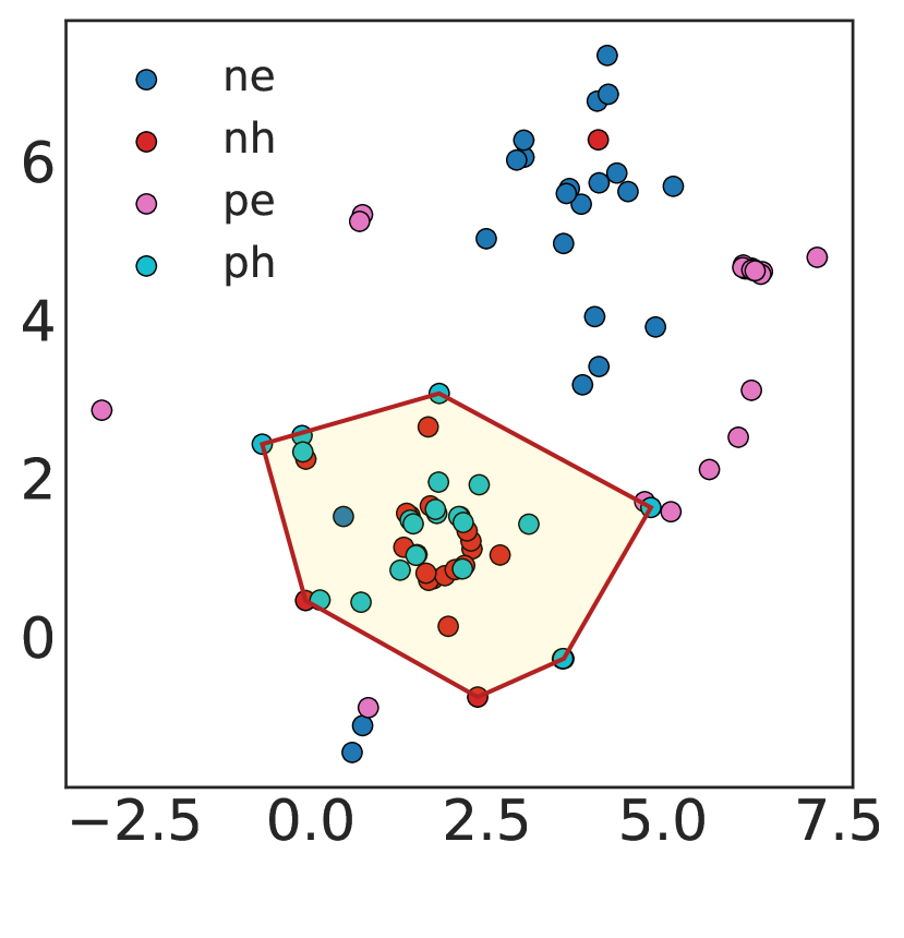
(a) Factor distribution in $\mathbb{R}^{2}$

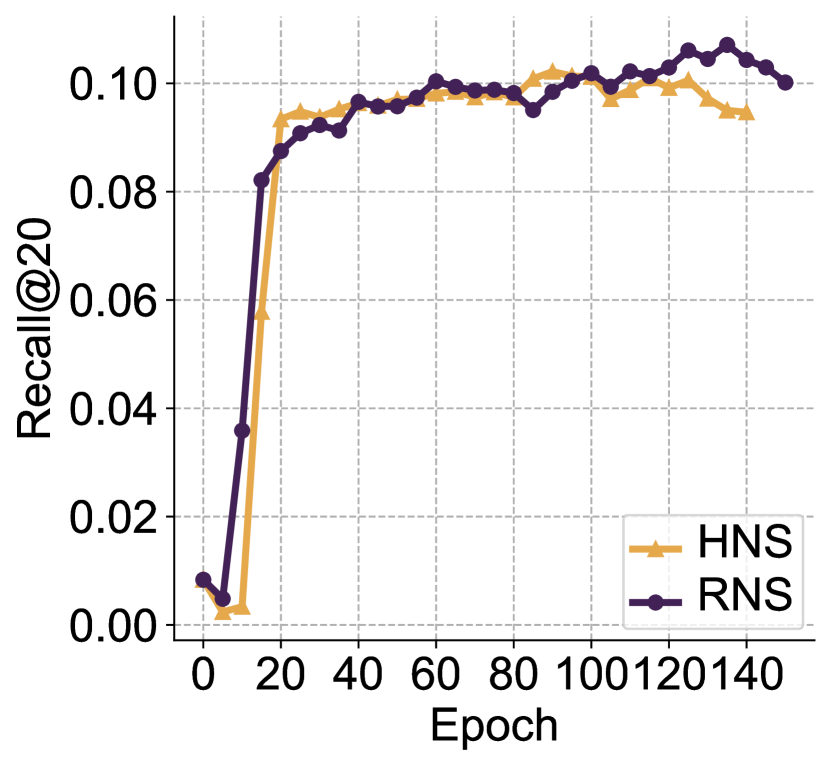
(b) Training curves

Figure 4. (a) shows the distribution of different factors learned by ANS on Last.fm. ne, nh, pe, and ph denote the $\mathbf{e}_{n}^{easy}$, $\mathbf{e}_{n}^{hard}$, $\mathbf{e}_{p}^{\prime}$, and $\mathbf{e}_{p}^{\prime\prime}$ respectively. (b) shows the training curves on Last.fm.

To verify the disentanglement performance, we spot-check a user and use the T-SNE algorithm (Van der Maaten and Hinton, 2008) to map the disentangled factors into a two-dimensional space. The results are shown in Figure 4(a). We can observe that $\mathbf{e}_{n}^{hard}$ and $\mathbf{e}_{p}^{\prime}$ are clustered together, confirming that they are indeed similar. In contrast, $\mathbf{e}_{n}^{easy}$ and $\mathbf{e}_{p}^{\prime\prime}$ are more scattered, indicating that they do not carry similar information, which is consistent with our previous analysis.

The hard factors should contain most of the useful information of negative items, and thus if we use only hard factors, instead of the entire original item, to train a model, we should achieve similar performance. We validate it by two experiments. First, we plot the curves of $Recall@20$ in Figure 4(b). HNS is a variant of RNS, which uses our disentanglement step to extract the hard factors of items and then uses only hard factors to train the model. It can be observed that the performance of HNS is comparable to that of RNS. The two curves are similar, confirming that the hard factors indeed capture the most useful information of negative items. Second, we revisit Figure 2 in Section 3.3. It can be seen that $\operatorname{PER}(\textrm{RNS},\textrm{HNS})$ is small, which means that HNS captures most of information learned in RNS.

In summary, our disentanglement step can effectively disentangle a negative sample into hard and easy factors, which lays a solid foundation for the subsequent steps in ANS.

5.4. RQ3: Ambiguous Trap and Information Discrimination

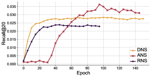
Figure 5. The curves of $Recall@20$ on the baby dataset.

5.4.1. Ambiguous Trap

Demonstrating how ANS can mitigate the ambiguous trap is a challenging task. A first attempt is to show the augmentation gain of the augmented negative samples. However, this idea is flawed because larger augmentation gain cannot always guarantee better performance (e.g., larger augmentation gain can be achieved by introducing a large number of false positive items). Therefore, we choose to analyze the curves of $Recall@20$ to show how ANS can mitigate the ambiguous trap, which is shown in Figure 5. Generally, the steeper the curve is, the more information the model can learn in this epoch from negative samples. We can observe that DNS outperforms RNS because its $Recall@20$ is always higher than that of RNS and the curve is steeper than that of RNS. It again confirms that hard negative sampling is an effective sampling strategy. In contrast, the curve of ANS exhibits distinct patterns. At the beginning (from epoch 0 to epoch 30), $Recall@20$ is low because ANS needs extra efforts to learn how to disentangle and augment negative samples. As the training process progresses (from epoch 30 to epoch 95), ANS demonstrates a greater average gradient. This proves that ANS can generate harder synthetic negative samples, which can largely mitigate the ambiguous trap issue.

Table 4. The percentage of overlapping high-score items between DNS and ANS.

Dataset	Baby	Beauty	Toy	Last.fm
Overlapping	47.3%	49.0%	40.9%	38.1%

5.4.2. Information Discrimination

As for the information discrimination problem, we have shown that the disentanglement step can effectively extract the useful information from low-score items. However, we have not shown that ANS can select more low-score negative items in the training process. To this end, we analyze the percentages of overlapping negative samples between ANS and DNS. The results are presented in Table 4. Recall that DNS always chooses the negative items with the highest scores as the hard negative samples. A less than 50% overlapping indicates that ANS does sample more low-score negative items before the augmentation and effectively alleviates the information discrimination problem.

5.5. RQ4: Ablation Study

We analyze the effectiveness of different components in our model, and evaluate the performance of the following variants of our model: (1) ANS without disentanglement (ANS w/o dis). (2) ANS without augmentation gain (ANS w/o gain). (3) ANS without regulated direction (ANS w/o dir). (4) ANS without regulated magnitude (ANS w/o mag). It is noteworthy to state that the complete elimination of the augmentation step is not taken into consideration due to its equivalence to DNS.

The results are presented in Table LABEL:tab:ablation. We can observe that all components we propose can positively contribute to model performance. In particular, the results show that unconstrained augmentation (e.g., ANS w/o mag) cannot achieve meaningful performance. This fact confirms that the existing unconstrained augmentation techniques cannot be directly applied to CF.

Table 5. Ablation Study.

Dataset	Last.fm		Beauty
Method	Top-20		Top-20
	Recall	NDCG	Recall	NDCG
ANS w/o dis	0.1108	0.0936	0.0286	0.0155
ANS w/o gain	0.1269	0.1036	0.0305	0.0166
ANS w/o dir	0.1025	0.0806	0.0191	0.0106
ANS w/o mag	0.0056	0.0024	0.0018	0.0007
ANS	0.1282	0.1045	0.0323	0.0188

5.6. RQ5: Hyper-Parameter Sensitivity

5.6.1. Impact of $\gamma$

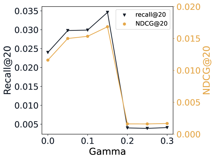
(a) Amazon-Baby

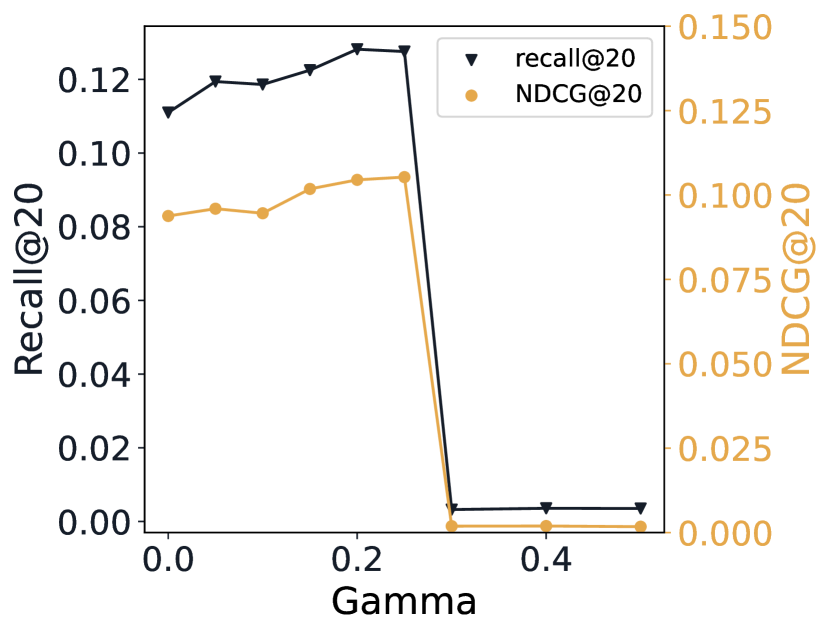
(b) Last.fm

Figure 6. Impact of $\gamma$ in ANS.

We present the effect of the weight of the contrastive loss and disentanglement loss, $\gamma$, in Figure 6. As the value of $\gamma$ increases, we can first observe notable performance improvements, which proves that both loss functions are beneficial for the CF model. It is interesting to observe that once $\gamma$ becomes larger than a threshold, the performance drops sharply. This observation is expected because in this case the CF model considers the disentanglement as the primary task and ignores the recommendation task. Nevertheless, ANS can achieve reasonable performance under a relatively wide range of $\gamma$ values.

5.6.2. Impact of $\epsilon$

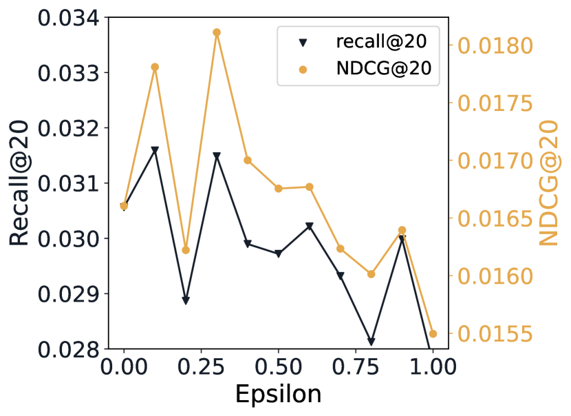
(a) Amazon-Baby

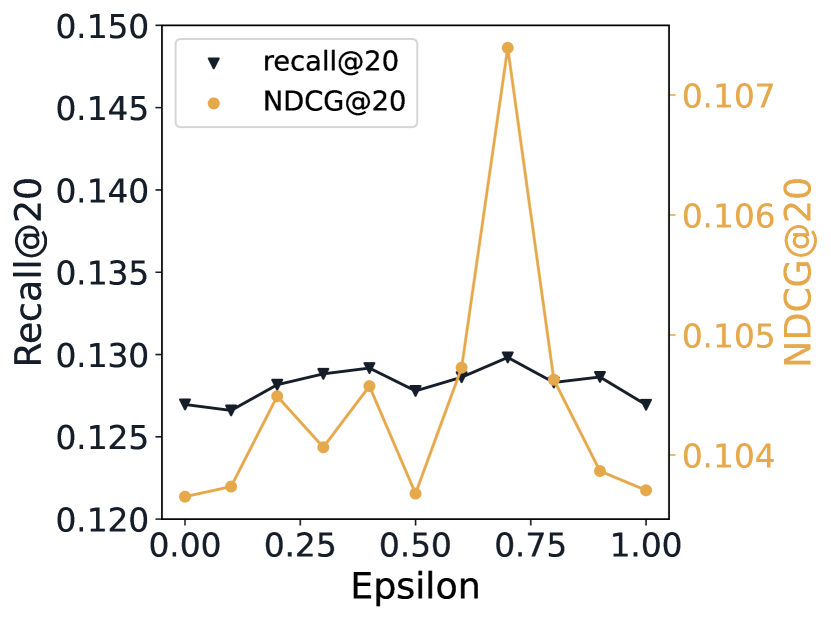
(b) Last.fm

Figure 7. Impact of $\epsilon$ in ANS.

Recall that $\epsilon$ is the parameter to balance the importance between the score and the augmentation gain in the sampling step. Figure 7(a) presents the results of different $\epsilon$ values. A small $\epsilon$ value overlooks the importance of the augmentation gain and only achieves sub-optimal performance; a large $\epsilon$ value may favor an item with a lower score (but a larger score difference), which will reduce the gradient and hurt model performance. But still, ANS can obtain good performance under a relatively wide range of $\epsilon$ values.

5.6.3. Impact of $M$

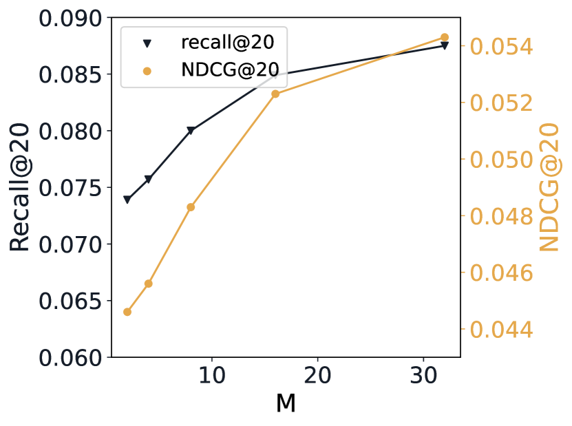
(a) Yelp

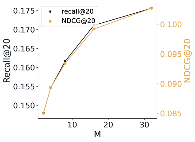
(b) Gowalla

Figure 8. Impact of $M$ in ANS.

$M$ denotes the size of candidate negative set $\mathcal{E}$. The present study illustrates the impact of $M$ on performance, as depicted in Figure 8. It is evident that an increase in $M$ leads to more negative samples, we can get harder negative samples by augmentation, thereby resulting in a performance improvement. Nevertheless, it is noteworthy that excessively large values of $M$ can considerably impede the efficiency of the models, and degrade performance due to noise (e.g., false negative samples).

5.7. RQ6: Efficiency Analysis

Table 6. Efficiency Analyses.

Dataset	Method	training time	epoch
Amazon-Beauty	RNS	0.47s	95
	DNS	0.64s	150
	ANS	0.89s	145
Gowalla	RNS	0.23s	90
	DNS	0.27s	80
	ANS	0.43s	140

Following the previous work (Wang et al., 2022; Mao et al., 2021), we also examine the efficiency of different negative sampling methods in Table 6. We report the average running time (in seconds) per epoch and the total number of epochs needed before reaching convergence. All three methods are relatively efficient. There is no wonder that RNS is the most efficient method as it is a model-agnostic strategy. Compared to DNS, our proposed ANS method requires more running time. However, considering the huge performance improvement ANS brings, the additional running time is well justified.

6. Conclusion

Motivated by ambiguous trap and information discrimination, from which the state-of-the-art negative sampling methods suffer, for the first time, we proposed to introduce synthetic negative samples from a fine-granular perspective to improve implicit CF. We put forward a novel generic augmented negative sampling (ANS) paradigm, along with a concrete implementation. The paradigm consists of three major steps. The disentanglement step disentangles negative items into hard and easy factors in the absence of supervision signals. The augmentation step generates synthetic negative items using carefully calibrated noise. The sampling step makes use of a new metric called augmentation gain to effectively alleviate information discrimination. Comprehensive experiments demonstrate that ANS can significantly improve model performance and represents an exciting new research direction.

In our future work, we intend to explore the efficacy of augmented negative samples in tackling various issues such as fairness and popularity bias. Additionally, we will actively investigate the effectiveness of employing augmented negative sampling in online experiments.

- (1)
- Bai et al. (2017) Yu Bai, Sally Goldman, and Li Zhang. 2017. Tapas: Two-pass Approximate Adaptive Sampling for Softmax. arXiv preprint arXiv:1707.03073 (2017).
- Bengio and Senécal (2008) Yoshua Bengio and Jean-Sébastien Senécal. 2008. Adaptive Importance Sampling to Accelerate Training of a Neural Probabilistic Language Model. IEEE Transactions on Neural Networks 19, 4 (2008), 713–722.
- Chen et al. (2020a) Jiawei Chen, Hande Dong, Xiang Wang, Fuli Feng, Meng Wang, and Xiangnan He. 2020a. Bias and Debias in Recommender System: Survey and Future Directions. arXiv preprint arXiv:2010.03240 (2020).
- Chen et al. (2022) Jin Chen, Defu Lian, Binbin Jin, Kai Zheng, and Enhong Chen. 2022. Learning Recommenders for Implicit Feedback with Importance Resampling. In Proceedings of the ACM Web Conference. 1997–2005.
- Chen et al. (2020b) Lei Chen, Le Wu, Richang Hong, Kun Zhang, and Meng Wang. 2020b. Revisiting Graph based Collaborative Filtering: A Linear Residual Graph Convolutional Network Approach. In Proceedings of the AAAI Conference on Artificial Intelligence, Vol. 34. 27–34.
- Chen et al. (2017) Ting Chen, Yizhou Sun, Yue Shi, and Liangjie Hong. 2017. On Sampling Strategies for Neural Network-based Collaborative Filtering. In Proceedings of the 23rd ACM SIGKDD International Conference on Knowledge Discovery and Data Mining. 767–776.
- Chin et al. (2022) Jin Yao Chin, Yile Chen, and Gao Cong. 2022. The Datasets Dilemma: How Much Do We Really Know About Recommendation Datasets?. In Proceedings of the 15th ACM International Conference on Web Search and Data Mining. 141–149.
- Ding et al. (2019) Jingtao Ding, Yuhan Quan, Xiangnan He, Yong Li, and Depeng Jin. 2019. Reinforced Negative Sampling for Recommendation with Exposure Data.. In International Joint Conference on Artificial Intelligence. 2230–2236.
- Ding et al. (2020) Jingtao Ding, Yuhan Quan, Quanming Yao, Yong Li, and Depeng Jin. 2020. Simplify and Robustify Negative Sampling for Implicit Collaborative Filtering. Advances in Neural Information Processing Systems 33 (2020), 1094–1105.
- Glorot and Bengio (2010) Xavier Glorot and Yoshua Bengio. 2010. Understanding the Difficulty of Training Deep Feedforward Neural Networks. In Proceedings of the 13th International Conference on Artificial Intelligence and Statistics. JMLR Workshop and Conference Proceedings, 249–256.
- Grover and Leskovec (2016) Aditya Grover and Jure Leskovec. 2016. Node2vec: Scalable Feature Learning for Networks. In Proceedings of the 22nd ACM SIGKDD International Conference on Knowledge Discovery and Data Mining. 855–864.
- Han et al. (2022) Tengyue Han, Pengfei Wang, Shaozhang Niu, and Chenliang Li. 2022. Modality Matches Modality: Pretraining Modality-Disentangled Item Representations for Recommendation. In Proceedings of the ACM Web Conference. 2058–2066.
- He et al. (2020) Xiangnan He, Kuan Deng, Xiang Wang, Yan Li, Yongdong Zhang, and Meng Wang. 2020. Lightgcn: Simplifying and Powering Graph Convolution Network for Recommendation. In Proceedings of the 43rd International ACM SIGIR Conference on Research and Development in Information Retrieval. 639–648.
- He et al. (2018) Xiangnan He, Zhankui He, Xiaoyu Du, and Tat-Seng Chua. 2018. Adversarial Personalized Ranking for Recommendation. In The 41st International ACM SIGIR Conference on Research & Development in Information Retrieval. 355–364.
- He et al. (2017) Xiangnan He, Lizi Liao, Hanwang Zhang, Liqiang Nie, Xia Hu, and Tat-Seng Chua. 2017. Neural Collaborative Filtering. In Proceedings of the 26th International Conference on World Wide Web. 173–182.
- Huang et al. (2021) Tinglin Huang, Yuxiao Dong, Ming Ding, Zhen Yang, Wenzheng Feng, Xinyu Wang, and Jie Tang. 2021. MixGCF: An Improved Training Method for Graph Neural Network-based Recommender Systems. In Proceedings of the 27th ACM SIGKDD Conference on Knowledge Discovery & Data Mining. 665–674.
- Kalantidis et al. (2020) Yannis Kalantidis, Mert Bulent Sariyildiz, Noe Pion, Philippe Weinzaepfel, and Diane Larlus. 2020. Hard Negative Mixing for Contrastive Learning. Advances in Neural Information Processing Systems 33 (2020), 21798–21809.
- Kang et al. (2022) SeongKu Kang, Dongha Lee, Wonbin Kweon, Junyoung Hwang, and Hwanjo Yu. 2022. Consensus Learning from Heterogeneous Objectives for One-Class Collaborative Filtering. In Proceedings of the ACM Web Conference. 1965–1976.
- Khosla et al. (2020) Prannay Khosla, Piotr Teterwak, Chen Wang, Aaron Sarna, Yonglong Tian, Phillip Isola, Aaron Maschinot, Ce Liu, and Dilip Krishnan. 2020. Supervised Contrastive Learning. Advances in Neural Information Processing Systems 33 (2020), 18661–18673.
- Kingma and Ba (2015) Diederik P. Kingma and Jimmy Ba. 2015. Adam: A Method for Stochastic Optimization. In 3rd International Conference on Learning Representations.
- Lai et al. (2023) Riwei Lai, Li Chen, Yuhan Zhao, Rui Chen, and Qilong Han. 2023. Disentangled Negative Sampling for Collaborative Filtering. In Proceedings of the Sixteenth ACM International Conference on Web Search and Data Mining. 96–104.
- Mao et al. (2021) Kelong Mao, Jieming Zhu, Jinpeng Wang, Quanyu Dai, Zhenhua Dong, Xi Xiao, and Xiuqiang He. 2021. SimpleX: A Simple and Strong Baseline for Collaborative Filtering. In Proceedings of the 30th ACM International Conference on Information & Knowledge Management. 1243–1252.
- Mikolov et al. (2013) Tomas Mikolov, Ilya Sutskever, Kai Chen, Greg S Corrado, and Jeff Dean. 2013. Distributed Representations of Words and Phrases and Their Compositionality. Advances in Neural Information Processing Systems 26 (2013).
- Park and Chang (2019) Dae Hoon Park and Yi Chang. 2019. Adversarial Sampling and Training for Semi-Supervised Information Retrieval. In The World Wide Web Conference. 1443–1453.
- Rendle and Freudenthaler (2014) Steffen Rendle and Christoph Freudenthaler. 2014. Improving Pairwise Learning for Item Recommendation from Implicit Feedback. In Proceedings of the 7th ACM International Conference on Web Search and Data Mining. 273–282.
- Rendle et al. (2009) Steffen Rendle, Christoph Freudenthaler, Zeno Gantner, and Lars Schmidt-Thieme. 2009. BPR: Bayesian Personalized Ranking from Implicit Feedback. In Proceedings of the 25th Conference on Uncertainty in Artificial Intelligence. AUAI Press, 452–461.
- Shi et al. (2023) Wentao Shi, Jiawei Chen, Fuli Feng, Jizhi Zhang, Junkang Wu, Chongming Gao, and Xiangnan He. 2023. On the Theories Behind Hard Negative Sampling for Recommendation. In Proceedings of the ACM Web Conference. 812–822.
- Srivastava et al. (2017) Akash Srivastava, Lazar Valkov, Chris Russell, Michael U Gutmann, and Charles Sutton. 2017. Veegan: Reducing Mode Collapse in Gans using Implicit Variational Learning. Advances in Neural Information Processing Systems 30 (2017).
- Thanh-Tung and Tran (2020) Hoang Thanh-Tung and Truyen Tran. 2020. Catastrophic Forgetting and Mode Collapse in Gans. In International Joint Conference on Neural Networks. IEEE, 1–10.
- Van der Maaten and Hinton (2008) Laurens Van der Maaten and Geoffrey Hinton. 2008. Visualizing Data Using T-SNE. Journal of Machine Learning Research 9, 11 (2008).
- Wang et al. (2022) Chenyang Wang, Yuanqing Yu, Weizhi Ma, Min Zhang, Chong Chen, Yiqun Liu, and Shaoping Ma. 2022. Towards Representation Alignment and Uniformity in Collaborative Filtering. In Proceedings of the 28th ACM SIGKDD Conference on Knowledge Discovery and Data Mining. 1816–1825.
- Wang et al. (2020) Jianling Wang, Kaize Ding, Liangjie Hong, Huan Liu, and James Caverlee. 2020. Next-item recommendation with sequential hypergraphs. In Proceedings of the 43rd international ACM SIGIR conference on research and development in information retrieval. 1101–1110.
- Wang et al. (2017) Jun Wang, Lantao Yu, Weinan Zhang, Yu Gong, Yinghui Xu, Benyou Wang, Peng Zhang, and Dell Zhang. 2017. IRGAN: A Minimax Game for Unifying Generative and Discriminative Information Retrieval Models. In Proceedings of the 40th International ACM SIGIR Conference on Research and Development in Information Retrieval. 515–524.
- Wang et al. (2021) Wenjie Wang, Fuli Feng, Xiangnan He, Liqiang Nie, and Tat-Seng Chua. 2021. Denoising Implicit Feedback for Recommendation. In Proceedings of the 14th ACM International Conference on Web Search and Data Mining. 373–381.
- Wang et al. (2019) Xiang Wang, Xiangnan He, Meng Wang, Fuli Feng, and Tat-Seng Chua. 2019. Neural Graph Collaborative Filtering. In Proceedings of the 42nd International ACM SIGIR Conference on Research and Development in Information Retrieval. 165–174.
- Wu et al. (2019) Ga Wu, Maksims Volkovs, Chee Loong Soon, Scott Sanner, and Himanshu Rai. 2019. Noise Contrastive Estimation for One-Class Collaborative Filtering. In Proceedings of the 42nd International ACM SIGIR Conference on Research and Development in Information Retrieval. 135–144.
- Wu et al. (2021) Jiancan Wu, Xiang Wang, Fuli Feng, Xiangnan He, Liang Chen, Jianxun Lian, and Xing Xie. 2021. Self-Supervised Graph Learning for Recommendation. In Proceedings of the 44th International ACM SIGIR Conference on Research and Development in Information Retrieval. 726–735.
- Xia et al. (2021) Xin Xia, Hongzhi Yin, Junliang Yu, Qinyong Wang, Lizhen Cui, and Xiangliang Zhang. 2021. Self-Supervised Hypergraph Convolutional Networks for Session-based Recommendation. In Proceedings of the AAAI Conference on Artificial Intelligence, Vol. 35. 4503–4511.
- Yang et al. (2020) Zhen Yang, Ming Ding, Chang Zhou, Hongxia Yang, Jingren Zhou, and Jie Tang. 2020. Understanding Negative Sampling in Graph Representation Learning. In Proceedings of the 26th ACM SIGKDD International Conference on Knowledge Discovery & Data Mining. 1666–1676.
- Yu et al. (2022) Junliang Yu, Hongzhi Yin, Xin Xia, Tong Chen, Lizhen Cui, and Quoc Viet Hung Nguyen. 2022. Are Graph Augmentations Necessary? Simple Graph Contrastive Learning for Recommendation. In Proceedings of the 45th International ACM SIGIR Conference on Research and Development in Information Retrieval. 1294–1303.
- Zhang et al. (2013) Weinan Zhang, Tianqi Chen, Jun Wang, and Yong Yu. 2013. Optimizing Top-N Collaborative Filtering via Dynamic Negative Item Sampling. In Proceedings of the 36th International ACM SIGIR Conference on Research and Development in Information Retrieval. 785–788.
- Zhao et al. (2021) Wayne Xin Zhao, Shanlei Mu, Yupeng Hou, Zihan Lin, Yushuo Chen, Xingyu Pan, Kaiyuan Li, Yujie Lu, Hui Wang, Changxin Tian, et al. 2021. Recbole: Towards a unified, comprehensive and efficient framework for recommendation algorithms. In Proceedings of the 30th ACM International Conference on Information & Knowledge Management. 4653–4664.
- Zheng et al. (2022) Yu Zheng, Chen Gao, Jianxin Chang, Yanan Niu, Yang Song, Depeng Jin, and Yong Li. 2022. Disentangling Long and Short-Term Interests for Recommendation. In Proceedings of the ACM Web Conference. 2256–2267.
- Zhu et al. (2022) Qiannan Zhu, Haobo Zhang, Qing He, and Zhicheng Dou. 2022. A Gain-Tuning Dynamic Negative Sampler for Recommendation. In Proceedings of the ACM Web Conference. 277–285.
- Zhuo et al. (2022) Jianhuan Zhuo, Qiannan Zhu, Yinliang Yue, and Yuhong Zhao. 2022. Learning Explicit User Interest Boundary for Recommendation. In Proceedings of the ACM Web Conference. 193–202.