SOLVING EQUILIBRIUM PROBLEMS IN ECONOMIES WITH FINANCIAL MARKETS, HOME PRODUCTION, AND RETENTION

Julio Deride		Roger J-B Wets
Department of Mathematics		Department of Mathematics
Universidad Técnica Federico Santa María		University of California, Davis
julio.deride@usm.cl		rjbwets@ucdavis.edu

Abstract. We propose a new methodology to compute equilibria for general equilibrium problems on exchange economies with real financial markets, home-production, and retention. We demonstrate that equilibrium prices can be determined by solving a related maxinf-optimization problem. We incorporate the non-arbitrage condition for financial markets into the equilibrium formulation and establish the equivalence between solutions to both problems. This reduces the complexity of the original by eliminating the need to directly compute financial contract prices, allowing us to calculate equilibria even in cases of incomplete financial markets.

We also introduce a Walrasian bifunction that captures the imbalances and show that maxinf-points of this function correspond to equilibrium points. Moreover, we demonstrate that every equilibrium point can be approximated by a limit of maxinf points for a family of perturbed problems, by relying on the notion of lopsided convergence.

Finally, we propose an augmented Walrasian algorithm and present numerical examples to illustrate the effectiveness of this approach. Our methodology allows for efficient calculation of equilibria in a variety of exchange economies, and has potential applications in finance and economics.
Keywords:  Walras equilibrium, stochastic equilibrium, lopsided convergence, general equilibrium              theory, augmented Walrasian, incomplete markets, GEI, no-arbitrage. JEL Classification:  C680, D580, C620 Date:

1 Introduction

In this paper, we investigate the computational challenges of solving general equilibrium problems for economies with real asset markets, home production, and retention, including the case when financial markets are incomplete. We follow the model in [18], where economic equilibrium for incomplete financial markets in general real assets is developed in a new formulation with currency-denominated prices. This model is an extension of the classic Walrasian economic equilibrium model presented by Arrow-Debreu [1], where agents optimize individually under perfect competition, and markets clear. In particular, we consider an inter-temporal economy, where agents face uncertainty over the future, and can make financial decisions by accessing a collection of real assets. Each agent also has access to domestic technologies to transform goods inter periods and, in addition, has the possibility of deciding to retain goods. In this setting, we focus our attention on the design of a methodology for finding equilibrium prices, following an optimization approach to the equilibrium problem.

Solving general equilibrium problems requires the use of numerical methods to solve optimization problems that, in the more realistic models, contain utility functions or a financial market structure that lead to difficulties in the computation, such as nonconvexities, nonsmoothness and unboundedness. The classic solution strategies rely heavily on stringent assumptions, such as interior initial endowments, differentiability, and constraint qualifications, in order to give a characterization of the equilibrium points using a differential topology framework. We propose an algorithm that works under weaker assumptions, and that follows a different approach from classical methods, relying on sequentially solving optimization problems.

The first computational methods presented to solve pure exchange economy equilibrium problems, where constructed by using a characterization of the equilibrium prices as the solutions of a fixed point problem. The most relevant solution strategies can be summarized in four main areas: Simplicial methods, proposed by Scarf [30], based on fixed point description of the problem, followed by an enumerative argument exploiting the geometry of the simplex of prices; Global Newton methods, where the equilibrium problem is presented as a dynamical system for the price vector, and it’s solved by Newton’s iterations; Homotopy methods, where the equilibrium state is seen as the solution of an extended system of nonlinear equations, describing optimality and market clearing conditions, in a collection of nonlinear equations. These methods are the most popular, and the solution strategy in this case is based on homotopy methods that solves iteratively a sequence simple problems that are homotopic to the original one, and are specially developed for models that incorporate incomplete financial markets (see [29] for homotopy methods, [12, 35] for GEI and pre-GEI models; [37, 36] for a smooth homotopy for GEI; [9, 4, 6, 10, 17, 16, 24] for computational approaches; and [11] for a Lemke’s scheme with separable piecewise linear concave utility functions). Finally, Optimization methods represents the equilibrium prices as the (direct) solution points of an optimization problem, solved by an Interior point method [5], or by an augmented Lagrangian method [32] (some references and details are omitted for the sake of simplicity on the exposition). Also, a family of methods based on tools from Variational Analysis and generalized equations have been proposed, for example, solving the equilibrium problem via a virtual market coordinator and epigraphical convergence [3], a generalized Nash game (GNEP) for risk-averse stochastic equilibrium problems [23], and the stochastic variational scheme presented in [26, 8].

We propose a solution strategy that is based on the correspondence between equilibrium prices and the (local) saddle points of the Walrasian bifunction. This idea extends our previous work on equilibrium problems [7], where our approach exhibits an alternative with theoretical advantages in terms of stability and satisfactory performance in terms of numerical analysis. We now incorporate a broader class of economic models, where the inclusion of financial markets, home production and retention is considered. Moreover, we provide a convergence proof for our algorithm based on the notion of lopsided convergence for bifunctions and design a version of our augmented Walrasian algorithm for this class of economies.

This article is organized as follows: in Section 2 we provide a mathematical description of the equilibrium model with financial markets, home production, and retention. Particularly, we describe the agent optimization problem, and characterize the financial markets. In Section 3 we study equilibrium conditions, and the formulation of the problem as a maxinf optimization type. Additionally, we present our approximation approach, along with our solution method. Finally, Section 4 illustrate our algorithm’s applicability, including example with it computational implementation of our results.

2 General equilibrium with financial markets model

The model described in this section corresponds to an extension to the general equilibrium model with real financial markets and retainability described on [18], where we incorporate home production. This addition enriches the model without adding technical complications. Hence, the original model in its form could have included it by loading up the notation. Basically, we consider a two-stage pure exchange economy, where agents decide on consumption, but also on financial assets, where outcomes on the second stage are uncertain.

2.1 Economy description

Consider an economy ${\cal E}$ with a finite number of heterogeneous agents, indexed by $i=1,\ldots,I$. They trade goods in a market operating in two stages, where the present or first stage is denoted by $\xi=0$, and there is uncertainty about the outcomes in the second stage, where a finite number of possible scenarios is considered, indexed by $\xi=1,\ldots,\Xi$. Goods or commodities, as in [18], are generalized goods and can be perishable or durable. We consider a finite number of commodities, indexed by $l=0,\ldots,L$.

Agents $i=1,\ldots,I$ are endowed with an initial bundle of goods $e^{i}=(e^{i}_{0},e^{i}_{1},\ldots,e^{i}_{\Xi})$, and they trade their holdings optimizing their preferences over goods, modeled by an utility function. This function takes into consideration the inter-temporal decision under uncertainty over the possibility of consumption and retention. Retainability of a particular good reflects the desirability of buying it for possibly later enjoyment, and it can happen on both stages. Thus, the utility function that captures this preferences is defined as a function of two variables: consumption, represented by $c^{i}=(c^{i}_{0},c^{i}_{1},\ldots,c^{i}_{\Xi})$, and retention, $w^{i}=(w^{i}_{0},w^{i}_{1},\ldots,w^{i}_{\Xi})$. Moreover, each agent has at his disposition the bundle of goods retained in the first stage (if any), where its availability depends on the second stage scenario, modeled by a matrix multiplication. Namely, if agents retain $w^{i}_{0}$ at the first stage, then, they have available an amount of $A_{\xi}w^{i}_{0}$ at scenario $\xi$ of the second stage. One example of this can be taken from the consumption of wine: it can be consumed on the first period, or can be retained for the next period, where a lucky consumer will get a better wine, or in a undesirable outcome, it can result in vinegar. Another example can be drawn from art, where buying a painting from an unknown artist can be enjoyed by its own merits, but if that artist becomes the next Michelangelo, the retained painting turns out to be more valuable.

Denote this utility function by $U^{i}:{I\kern-3.50006ptR}_{+}^{(1+L)\times(1+\Xi)}\times{I\kern-3.50006ptR}_{+}^{(1+L)\times(1+\Xi)}\to\overline{I\kern-3.50006ptR}$, and assume its upper semicontinuity (usc), with a survival set given by $C^{i}={\rm dom}\,U^{i}=\big{\{}(c,w){\,\big{|}\,}U^{i}(c,w)<\infty\big{\}}$. For example, we consider agents that are maximizing their expected utility, i.e., their objective function takes the following form

$$U^{i}(c,w)=u^{i}(c_{0},w_{0})+{I\kern-3.50006ptE}\{u^{i}(c_{\mbox{\boldmath$\xi$}},w_{\mbox{\boldmath$\xi$}})\},$$

for $u^{i}:{I\kern-3.50006ptR}_{+}^{(1+L)}\times{I\kern-3.50006ptR}_{+}^{(1+L)}\to\overline{I\kern-3.50006ptR}$.

In this economy, agents have access to home production technology, described as a process consisting of a collection of activities that requires a bundle of goods as input, and produce an (stochastic) bundle of output goods in the second stage. This procedure is modeled by a decision variable $y$ that belongs to a set of acceptable activities, and pair of input/output matrices $(T^{i}_{0},\{T^{i}_{\mbox{\boldmath$\xi$}}\})$ that are at the disposal of agent-$i$. Thus, by using $T^{i}_{0}y$ resources, a random output of $T^{i}_{\mbox{\boldmath$\xi$}}y$ is obtained at the second stage. We assume that the set of acceptable activities, $Y^{i}\subset{I\kern-3.50006ptR}^{m}_{+}$, is a closed convex cone, and it includes the possibility of no-action, i.e., $0\in Y^{i}$. One possible interpretation for the matrices determining the input/output (home production), is considering it as process that could simply be savings (including enhancements or deterioration), investment activities, retention, and so on.

On the other hand, the financial markets structure considered in this economy is detailed as follows. The agents have access to a finite number of contracts, indexed by $j=0,\ldots,J$, where each contract $j=0,\ldots,J$ has an associated return vector of goods, depending on the outcome in the second stage. Fixing notation, for each unit of the $j$ marketed asset, the stochastic return delivered is described by a bundle of goods denoted by $D_{j,\mbox{\boldmath$\xi$}}$. We are not imposing any explicit restrictions on financial transactions happening simultaneously. However, additional provisions for each transaction (real transaction costs) are modeled by an associated cost vector of goods $D_{0}$ for every unit of contract that is issued (sold).

Under this market characterization, and without providing any further description of the uncertainty, the market information structure is organized as a tree, as depicted in Figure 1.

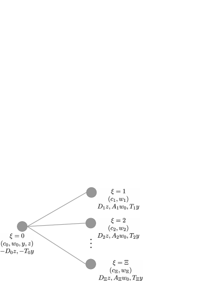
Figure 1: Market structure of GEI model. First stage decision variables of consumption, retention, home production, and financial portfolio are summarized by $(c_{0},w_{0},y,z)$ respectively, along with associated transactional cost of $-D_{0}z$ and home production input $-T_{0}y$. At the second stage (and for each scenario), the consumption and retention variables are $(c_{\xi},w_{\xi})$; and financial, retainability, and production outcomes are represented by $(D_{\xi}z,A_{\xi}w_{0},T_{\xi}y)$.

The last element to fully describe the economy are prices. Goods and contracts are traded in a perfect market competition setting. We denote the market prices of goods by $p=(p_{0},p_{1},\ldots,p_{\Xi})\in{I\kern-3.50006ptR}_{+}^{(1+L)\times(1+\Xi)}$, and the market prices of financial contracts by $q=(q_{0},q_{1},\ldots,q_{J})\in{I\kern-3.50006ptR}_{+}^{1+J}$. Hence, under perfect competition, agents are price taker, and given prices $p$ and $q$, each agent $i$ chooses an affordable bundle of consumption goods $c^{i}$, a retention strategy $w^{i}$, and a financial decision given by a portfolio strategy $z^{i}=z^{i+}-z^{i-}$ that maximize their utility function. Thus, each agent solves the following optimization problem

$$\max_{\{c,w,y,z^{+},z^{-}\}} \;U^{i}\left(w,c\right)$$

$${\rm s.t.} \;\langle p_{0},\,c_{0}+w_{0}+D_{0}z^{-}+T^{i}_{0}y\rangle+\langle q,z^{+}\rangle\leq\langle p_{0},\,e^{i}_{0}\rangle+\langle q,\,z^{-}\rangle$$

$$\langle p_{\xi},\,c_{\xi}+w_{\xi}+D_{\xi}z^{-}\rangle\leq\langle p_{\xi},\,e^{i}_{\xi}+D_{\xi}z^{+}+A^{i}_{\xi}w_{0}+T^{i}_{\xi}y\rangle,\xi=1,\ldots,\Xi$$

$$(c,w)\in C^{i},\,z^{+},z^{-}\in{I\kern-3.50006ptR}^{1+J}_{+},\,y\in Y^{i}.$$

Let $(c^{i},w^{i},y^{i},z^{+,i},z^{-,i})$ be a solution for this problem (depending on $p$ and $q$). In order to ease the notation, let’s define the individual excess supply as

$$\begin{cases}s^{i}_{0}&=\;e^{i}_{0}-c^{i}_{0}-w^{i}_{0}-D_{0}z^{-,i}-T^{i}_{0}y^{i},\\ s^{i}_{\xi}&=\;e^{i}_{\xi}+D_{\xi}(z^{+,i}-z^{-,i})+A^{i}_{\xi}w^{i}_{0}+T^{i}_{\xi}y^{i}-c^{i}_{\xi}-w^{i}_{\xi},\,\xi=1,\ldots,\Xi\end{cases}$$ (1)

For this economy, we define the Excess Supply function as the difference between the aggregate supply and the aggregate demand. In our case, it is defined as follows

$${\rm ES}_{0}=\sum_{i=1}^{I}s^{i}_{0},\quad{\rm ES}_{\xi}=\sum_{i=1}^{I}s^{i}_{\xi},\,\xi=1,\ldots,\Xi,$$

Given the excess supply functions $\{{\rm ES}_{\xi}\}$, we define an equilibrium for the economy as price vector, $(p,q)$ such that this family of functions are non-negative,

$${\rm ES}_{\xi}\geq 0,\,\xi=0,\ldots,\Xi,$$

i.e., at equilibrium, the market is capable of satisfying the aggregate demand of goods with the available aggregate supply. On the other hand, we require that at these price vector, the market of financial contracts clears,

$$\sum_{i}z^{+,i}=\sum_{i}z^{-,i},$$

where the total amount of financial contracts issued is equal to the number of contracts purchased, or the aggregate short positions are equal to the aggregate long positions.

Before we proceed with further details of the model, let’s state one assumption regarding the desirability of the available goods in the economy, and another assumption regarding survivability of the agents.

2.1 Assumption

(indispensibality). There is a good that is indispensable to all agents. Every good is indispensable to at least one agent.

This assumption is weaker that the classic strong monotonicity assumption [25], as it only reinforce the indispensability of the same good for every agent, and guarantees that the goods traded in the economy are actually desired for at least one agent. Denote the indispensable good for all agents by the first indexed good ($l=0$). We will use this good as the numéraire for this economy for every scenario of the economy. Therefore, assume that $p_{\xi,0}=1,\,\xi=0,\ldots,\Xi$ (a different approach can be followed by imposing that $p_{\xi}\in\Delta_{L+1},\,\xi=0,\ldots,\Xi$, where $\Delta_{n}$ corresponds to the $n$-dimensional canonical simplex). Another advantage of this approach is that it helps up to avoid indeterminacy of the price system, and, therefore, ease the comparison between prices for different stages.

Additionaly, the stochastic nature of the agents’ problems requires survival assumptions with respect to the survivability condition or market partipicipation. Following the approach in [18], we adopt the following assumption

2.2 Assumption

(ample survivability assumption) For every agent $i$, and for all possible scenarios $\xi=1,\ldots,\Xi$, there exists a consumption bundle $(\tilde{c}^{i},\tilde{w}^{i})\in C^{i}$, and an activity level $\tilde{y}\in Y^{i}$, such that

$$e^{i}_{0}-\tilde{c}^{i}_{0}-\tilde{w}^{i}_{0}-T^{i}_{0}\tilde{y} \geq 0,$$

$$e^{i}_{\xi}-\tilde{c}^{i}_{\xi}-\tilde{w}^{i}_{\xi}+T^{i}_{\xi}\tilde{y}+A_{\xi}\tilde{w}^{i}_{0} \geq 0,\,\xi=1,\ldots,\Xi$$

Mathematically, these conditions correspond to the relatively complete recourse property, and they guarantee the feasibility of each agents’ problem. From the economic perspective, this assumption provides a minimum requirement for each agent to be able to engage in trading, and participate in the economy, independently of the market prices.

2.2 No-Arbitrage condition

We base our equilibrium approach on prices that satisfy the no-arbitrage condition, in order to rule out the existence of arbitrage opportunities on the financial markets (for example, [22, Ch.5,§3.3]). Simply put, this condition relates the prices of the financial contracts and their associated returns. A trading strategy that delivers a (at least one) positive payoff, without requiring any payment is called arbitrage. Formally, the no-arbitrage condition is stated as

$$\mbox{ there is no }\,z\in{I\kern-3.50006ptR}^{1+J}\,\mbox{ such that }\,\langle q,z\rangle<0,\quad\,W_{1}(p)z:=\left[\begin{array}[]{c}p_{1}^{T}D_{1}\\ \vdots\\ p_{\Xi}^{T}D_{\Xi}\end{array}\right]z>0.$$

The matrix $W_{1}(p)$ defines the span of the financial market at price $p$. By defining $W(p,q)=\left[\begin{array}[]{c}-q^{T}\\ W_{1}(p)\end{array}\right]$, the non-arbitrage condition is interpreted as the existence of no portfolios such that $Wz>0$. Equivalently, following a similar approach to [25, Thm.9.3], this condition can be re-stated as

$$\langle W\rangle\cap\Delta_{\Xi+1}=\emptyset$$

As $\Delta_{\Xi+1}$ is a compact set, and $\langle W\rangle$ is a closed subspace, then there exists an strictly separating hyperplane defined by a normal vector $\sigma\neq 0$, such that

$$\sup_{\tau\in\langle W\rangle}\sigma\cdot\tau<\,\inf_{\tau\in\Delta_{\Xi+1}}\sigma\cdot\tau$$

Moreover, $\sigma\in{I\kern-3.50006ptR}_{++}^{1+\Xi}$ and $\sigma\in\langle W\rangle^{\perp}$, i.e., $\sigma_{\xi}>0,\xi=0,\ldots,\Xi$ and $\sigma\cdot\,W\,z=0,\forall z$. Finally, (redefining $\sigma\leftarrow\frac{\sigma}{\sigma_{0}}$ if necessary) the no-arbitrage condition can be stated as the existence of positive scalars $\sigma_{\xi}>0,\xi=1,\ldots,\Xi$ such that

$$q=\sum_{\xi=1}^{\Xi}\sigma_{\xi}\,D_{\xi}^{T}p_{\xi}$$ (2)

Therefore, any prices $p$ and $q$ that satisfy the non-arbitrage condition have (at least one) associated vector $\sigma$ such that the Equation (2) holds. The vector $\sigma$ is usually denoted as the vector of state prices or a vector that rationalizes the prices $p$ and $q$. In what follows, we only considered prices that satisfy this condition.

2.3 A solution strategy for the agents’ problems

We use the no-arbitrage condition to propose an alternative solution strategy for the equilibrium problem for this economy. Equilibrium conditions will be described in detail on the next section (Section (3)). However, we will focus our analysis on equilibrium prices that are free of arbitrage. Thus, let’s assume that $q$ and $p$ are no-arbitrage prices, rationalized by $\sigma$, and define an alternative vector of prices

$$\tilde{p}_{0}=p_{0},\quad\tilde{p}_{\xi}=\sigma_{\xi}p_{\xi},\xi=1,\ldots,\Xi$$ (3)

Note that with this transformation $\tilde{p}_{\xi,0}$ is no longer equal to 1, for $\xi=1,\ldots,\Xi$. In fact, $\tilde{p}_{\xi,0}$ correspond to the associated state price $\sigma_{\xi}$.

Additionally, let us introduce a natural bound on the consumption space, given by

$$c_{\xi},w_{\xi}\leq m:=\sup\Big{\{}\sum_{i=1}^{I}e^{i}_{\xi}{\,\Big{|}\,}\,\xi=1,\ldots,\Xi\Big{\}},\xi=0,\ldots,\Xi,\quad z^{+},z^{-}\leq M(>0),$$

where the first inequality follows by the individual consumption being bounded by the aggregate available goods. Note that this set of inequalities apply also to the retention decision variables. Under these assumptions, and under the no-arbitrage condition, the consumption set turns out to be compact [22, Ch.5,Thm.1]. Therefore, there is an upper bound on the financial contracts, that is represented with the second bound (note that this bound includes the potential goods produced by home-production). These considerations lead to the following formulation of the agent problem, written in terms of the individual excess supply $s_{\xi}$ and the new price system $\tilde{p}$ as

$$\max_{\{c,w,y,z^{+},z^{-}\}} \;U^{i}\left(w,c\right)$$ (4)

$${\rm s.t.} \;\langle{\tilde{p}}_{0},\,s_{0}\rangle-\sum_{\xi=1}^{\Xi}\langle{\tilde{p}}_{\xi},D_{\xi}(z^{+}-z^{-})\rangle\geq 0,$$

$$\langle{\tilde{p}}_{\xi},\,s_{\xi}\rangle\geq 0,\,\xi=1,\ldots,\Xi$$

$$(c,w)\in C^{i}\cap{I\kern-3.50006ptB}(0;\,m),\,z^{+},z^{-}\in[0,\,M],\,y\in Y^{i}.$$

A crucial observation comes from this substitution: the agent problem only depends on prices $\tilde{p}$ and is no longer dependent on the prices $q$. Thus, defining the equilibrium conditions for this new version and solving the equilibrium for $\tilde{p}$ reduces the dimension of the problem, and reduces its computational difficulty.

Remark. Under Assumption 2.1, it is easy to see that Walras’ law holds in this economy, and the budget constraints turns out to be active for every state $t=0,1,\ldots,\Xi$      

Finally, the last element for establishing the equilibrium problem under this new setting is the recovering process to obtain the corresponding prices for the original economy ($p,q$), based on prices for the modified problem $\tilde{p}$. Thus, let $\tilde{p}$ be an equilibrium price for the modified economy (a precise definition is the equilibrium for the modified economy is given in definition 3.1). First of all, we use the Equation (2) to obtain $q$ as follows:

$$q=\sum_{\xi=1}^{\Xi}D_{\xi}^{T}{\tilde{p}}_{\xi}.$$ (5)

From here, we compute the state prices (or multipliers) $\sigma$ that rationalize this system of prices by using the price normalization introduced in Equation (3),

$$p_{\xi,0}=1\iff\sigma_{\xi}=\tilde{p}_{\xi,0}.$$ (6)

Finally, the equilibrium price for commodities is determined by

$$p_{0}={\tilde{p}}_{0},\quad p_{\xi,0}=1,\,p_{\xi,l}=\frac{{\tilde{p}}_{\xi,l}}{{\tilde{p}}_{\xi,0}},\,l=1,\ldots,L,\,\xi=1,\ldots,\Xi.$$

Note that by using this procedure, we characterize equilibrium prices for goods and financial contracts for the original problem, $p$ and $q$, by computing the equilibrium prices for commodities of the auxiliary economy, $\tilde{p}$. Explicitly, the lack of financial contracts prices for the auxiliary economy has further implications on the family of equilibrium problems that can be solved. As mentioned before, GEI models exhibit difficulties when the matrix of financial returns drops rank, and in order to compute equilibrium points, an extra procedure to the classic homotopies has to be performed. However, our approach overcome this situation by considering prices on the manifold of no-arbitrage, and thus, we compute prices for a modified pure-exchange economy, where classic methods can be applied directly. Note that the concept of no-arbitrage equilibrium has been proposed before, for example by Hens in [22, Ch.5,§3.3], but it has not been used for computational purposes to the best of our knowledge.

The next step is to analyze the equilibrium conditions for the original economy, and provide the optimization characterization of equilibrium points, defining the Walrasian bifunction associated to this economy.

3 Equilibrium formulation and Approximation

In this section, we discuss the equilibrium conditions for this general equilibrium model. Consider an economy with normalized prices, and such that the no-arbitrage condition has been incorporated to the formulation of the agents’ utility maximization problem, i.e., the agents’ problems only depend on the alternative prices $\tilde{p}$ (as in Problem 4). Let us denote this modified economy as $\tilde{\cal E}$ and define the equilibrium conditions as follows

3.1 Definition

(equilibrium for the modified economy) Consider de modified economy $\tilde{\cal E}$. An equilibrium for this economy is given by a system of prices ${\tilde{p}}^{*}=({\tilde{p}}^{*}_{0};{\tilde{p}}^{*}_{1},\ldots,{\tilde{p}}^{*}_{\Xi})\in{I\kern-3.50006ptR}_{+}^{L}\times{I\kern-3.50006ptR}^{(L+1)\Xi}_{+}$, and individual excess supply allocations, $s^{i}=s^{i}({\tilde{p}}^{*})$, $i=1,\ldots,I$, defined as Equation (1) (depending on the optimal solutions $({c}^{i},w^{i},y^{i},{z}^{+,i},{z}^{+,i})$) such that

1. Utility maximization Agent $i$ maximizes the utility function $U^{i}$ over the set

   $${\cal B}^{i}({\tilde{p}}^{*})=\left\{(c,w,y,z^{+},z^{-})\left|\begin{array}[]{l}\displaystyle\langle{\tilde{p}}^{*}_{0},\,s_{0}^{i}\rangle-\sum_{\xi=1}^{\Xi}\langle{\tilde{p}}^{*}_{\xi},\,D_{\xi}(z^{+}-z^{-})\rangle\geq 0,\,\langle{\tilde{p}}^{*}_{\xi},\,s_{\xi}^{i}\rangle\geq 0,\xi=1,\ldots,\Xi\\ 0\leq c,w\leq m,\,y\in Y^{i},\,0\leq z^{+},z^{-}\leq M\end{array}\right.\right\}$$

   for every agent $i=1,\ldots,I$.

2. Commodity Markets Clearing The aggregate demand of goods at the prices ${\tilde{p}}^{*}$ do not exceed the aggregate supply in the first stage, as well as every possible state at the second stage, i.e.,

   $${\rm ES}_{\xi,l}\geq 0,\,l=0,\ldots,L,\,\xi=0,\ldots,\Xi$$

3. Financial Markets Clearing The market clearing condition for financial contracts, i.e.,

   $$\sum_{i=1}^{I}{z}^{+,i}_{j}=\sum_{i=1}^{I}{z}^{-,i}_{j},\,j=0,\ldots,J$$

Under this definition of equilibrium, we propose a solution procedure based on solving an associated optimization problem, following the approach proposed first in [21]. Here, equilibrium prices are characterized as maxinf points of a bifunction called Walrasian, that captures the market misbalance on aggregate excess supply at given prices. Thus, the first step to obtain the maxinf characterization is to define an associated Walrasian function for the modified economy. Define the domain of the price vector $\tilde{p}$ as the set $\Gamma:={I\kern-3.50006ptR}^{(1+L)(1+\Xi)-1}_{+}$ (as $\tilde{p}_{0}(0)=1$ is fixed). Additionally, defined the dual variables $\tilde{g}\in\Gamma$, and define the Walrasian $W:\Gamma\times\Gamma\to{I\kern-3.50006ptR}$ as follows

$$W({\tilde{p}},{\tilde{g}}) =\,\langle\,{\tilde{g}},\,\tilde{\rm ES}(\tilde{p})\,\rangle-\rho\left\|\sum_{i=1}^{I}z^{+,i}-z^{-,i}\right\|_{2}^{2},$$ (7)

$$=\sum_{\xi=0}^{\Xi}\sum_{{\begin{subarray}{c}l=0\\ (\xi,l)\neq(0,0)\end{subarray}}}^{L}{\tilde{g}}_{\xi,l}{\rm ES}_{\xi,l}(\tilde{p})-\rho\sum_{j=0}^{J}\left(\sum_{i=1}^{I}z_{j}^{+,i}-z_{j}^{-,i}\right)^{2},$$

for some positive parameter $\rho>0$, where $\tilde{\rm ES}(\tilde{p})$ corresponds to ${\rm ES}(\tilde{p})$ without the first component (${\rm ES}_{0,0}(\tilde{p})$).

In what follows, we are interested in relating equilibria with maxinf points of the Walrasian bifunction. One refers to $\tilde{p}$ a maxinf point of $W$ if

$${\tilde{p}}\in\mathop{\rm argmax}_{p\in\Gamma}\left[\inf_{g\in\Gamma}W(p,g)\right],$$

and, for $\varepsilon\geq 0$, $\tilde{p}_{\varepsilon}$ is called an $\varepsilon$-maxinf point of $W$, if

$$W(\tilde{p}_{\varepsilon},\cdot)\geq\mathop{\rm supinf}\nolimits W-\varepsilon.$$

The set of such points are denoted by $\mathop{\rm argmaxinf}\nolimits\,W$ and $\varepsilon$-$\mathop{\rm argmaxinf}\nolimits\,W$ respectively. Notice that the definition of $\varepsilon$-maxinf point is made over an approximation concept of the optimality of the function evaluation of $W$, and we will see later that this is the correct interpretation of an approximate maxinf point, in the context of an approximate equilibrium point.

Let us state the first result about the relationship between maxinf points of the Walrasian function, and equilibrium points for the economy.

3.2 Lemma

(Walras equilibrium prices and maxinf-points) Every maxinf-point ${\tilde{p}}\in\Gamma$ of the Walrasian bifunction $W$ such that ${\tilde{W}}({\tilde{p}},\cdot)\geq 0$ on $\Gamma$ is an equilibrium point.

Proof. Let $\tilde{p}$ be a maxinf-point of $W$ such that ${W}({\tilde{p}},\cdot)\geq 0$. Notice that, by Assumption 2.1, for any price $\tilde{p}$, the excess supply associated with the numéraire good (which is define as the one indispensable to all agents) has to be non-positive, i.e., ${\rm ES}_{0,0}\leq 0$. Moreover, taking ${\tilde{g}}=0\in\Gamma$,

$$0\leq W({\tilde{p}},0)=-\rho\sum_{j=0}^{J}\left(\sum_{i=1}^{I}z_{j}^{+,i}-z_{j}^{-,i}\right)^{2}\,\,\mbox{then}\,\,0=\sum_{i=1}^{I}z_{j}^{+,i}-z_{j}^{-,i},\,j=0,\ldots,J$$

which entails the equilibrium conditions for financial contracts. Aditionally, considering ${\tilde{g}}=e_{\xi,l}\in\Gamma$ the unit-price vector that assigns 1 to good $l$ at scenario $\xi$. Then,

$$0\leq{\tilde{W}}({\tilde{p}},e_{\xi,l})\leq{\rm ES}_{\xi,l},\,\xi=0,\ldots,\Xi,\,l=0,\ldots,L,(\xi,l)\neq(0,0),$$

providing the equilibrium conditions for those markets. Finally, the market clearing condition for the first good at first stage, $(\xi,l)=(0,0)$, follows from the aggregation of the (active) budget constraints for each agent at price $\tilde{p}$, and combine it with the Walras’ law and the inequality $W({\tilde{p}},{\tilde{p}})\geq 0$.

     

Using Lemma (3.2), we pose the problem of finding an equilibrium point as one of finding maxinf points for the Walrasian function. We propose a method to solve this problem by using the appropriate notion of convergence on the space of bifunctions, corresponding to the lopsided convergence. Following the same approach tha we initiated in [7], let’s build a family of approximating bifunctions that ancilliary lop-converges to the Walrasian bifunction. Lopsided convergence (ancillary tight) is aimed at the convergence of maxinf points, and in our context is defined as follows

3.3 Definition

(ancilliary-tight lopsided convergence). A sequence $\big{\{}W^{\nu}:\Gamma^{\nu}\times\Gamma^{\nu}\to{I\kern-3.50006ptR}\big{\}}_{\nu\in{I\kern-2.45004ptN}}$ lop-converges ancilliary tight to the function $W:\Gamma\times\Gamma\to{I\kern-3.50006ptR}$, if

(a)

for all $g\in\Gamma$, and all $(p^{\nu}\in\Gamma^{\nu})\to p\in\Gamma$, there exists $(g^{\nu}\in\Gamma^{\nu})\to g$ such that

$$\limsup_{\nu}W^{\nu}(p^{\nu},g^{\nu})\leq W(p,g),$$

(b)

for all $p\in\Gamma$, there exists $(p^{\nu}\in\Gamma^{\nu})\to p$ such that given any $(g^{\nu}\in\Gamma^{\nu})\to g$,

$$\liminf_{\nu}W^{\nu}(p^{\nu},g^{\nu})\geq W(p,g)\quad\mbox{when }g\in\Gamma\quad\mbox{and}\quad W^{\nu}(p^{\nu},g^{\nu})\to\infty\quad\mbox{when }g\notin\Gamma.$$

(b-t)

and for any $\epsilon>0$, one can find a compact set $K_{\epsilon}\neq\emptyset$ (possibly depending on $\big{\{}p^{\nu}\to p\big{\}}$) such that for all $\nu$ sufficiently large,

$$\inf_{\Gamma^{\nu}\cap K_{\epsilon}}W^{\nu}(p^{\nu},\cdot)\leq\inf_{\Gamma^{\nu}}W^{\nu}(p^{\nu},\cdot)+\epsilon.$$

We propose a family of approximating bifunctions, called augmented Walrasian, $\{W^{\nu}\}$, based on a non-concave augmentation technique. This construction is an extension of our previous work [7], and this family is defined for a non-decreasing family of scalars $\{r^{\nu}\}$, a non-decreasing family of vectors $\{K^{\nu}\}\subset\Gamma$, and an augmenting function $\sigma:\Gamma\to{I\kern-3.50006ptR}$. Consider the approximating domain $\Gamma^{\nu}=[0,K^{\nu}]\cap\Gamma$, and define ${W}^{\nu}:\Gamma^{\nu}\times\Gamma^{\nu}\to{I\kern-3.50006ptR}$ by

$${W}^{\nu}({\tilde{p}},{\tilde{g}})=\inf_{z}\Big{\{}{W}({\tilde{p}},{\tilde{g}}-z)+r^{\nu}\sigma^{*}\left(\frac{1}{r^{\nu}}z\right)\Big{\}}$$ (8)

3.4 Theorem

(upper-semi continuity of the Walrasian) If the agents’ utility maximization problem have a unique solution for every $\tilde{p}$, then the Walrasian function for the modified economy defined on Equation (7) is upper semi-continuous on its first argument, i.e., for fixed ${\tilde{g}}\in\Gamma$, $W(\cdot,{\tilde{g}})$ is usc.

Proof. For each agent $i$, define the variable $v=(c,w,y,z^{+},z^{-})$, and define the function (dropping the dependence on $i$)

$$f({\tilde{p}},v)=\begin{cases}U(c,w)&v\in{\cal B}({\tilde{p}})\\ -\infty&\mbox{otherwise}\end{cases},$$

and, define the function

$$P({\tilde{p}})=\mathop{\rm argmax}_{v}f({\tilde{p}},v),$$

which by hypothesis turns out to be single-valued. From here, it is easy to see that the solution to the agent’s problem correspond to the sup-projection of the function $f$ onto its $v$ variable, and in order to prove the usc of the Walrasian, we study the convergence properties of the function $P$. Note that $f$ is usc, proper, and $f$ is level-bounded in $v$ locally uniformly $\tilde{p}$, properties inherited by the utility function $U$ and compactness of ${\cal B}({\tilde{p}})$. Then, the map $P$ is continuous, in virtue of theorem [28, Thm7.41],[34], and the conclusion follows as ${\tilde{W}}(\cdot,{\tilde{g}})$ is a composition of continuous functions.      

3.5 Lemma

(Ky-Fan properties of the augmented Walrasian) The finite valued bifunctions $\{W^{\nu}\}$ (defined in (8)) are Ky-Fan bifunctions. Moreover, for every $\nu$ the set of maxinf points of $W^{\nu}$ is nonempty.

Proof. Recall that a bifunction $F:K\times K\to{I\kern-3.50006ptR}$ is a Ky-Fan function, if

• For every $y\in K$, the function $F(\cdot,y)$ is a usc, and

• For every $x\in K$, the function $F(x,\cdot)$ is convex.

The augmented Walrasian can be seen as the inf-projection of the function

$$({\tilde{p}},{\tilde{g}},z)\mapsto{W}({\tilde{p}},{\tilde{g}}-z)+r^{\nu}\sigma^{*}(r^{-1}z),$$

on the $z$-variable. Thus, the convexity condition (ii) is given by the application of [28, Thm.2.2]. In addition, for a fixed $\tilde{g}\in\Gamma^{\nu}$, the usc of $W^{\nu}$ is inherited from the usc of $W$ by Theorem 3.4. Finally the set ${\rm argmaxinf}\,{W}^{\nu}$ is non-empty by Ky-Fan inequality [2, Thm.8.6].      

3.6 Theorem

(lop-convergence of augmenting Walrasians) The sequence of augmented Walrasian bifuctions converges lopsided anciallary tightly to the original Walrasian, i.e., ${W}^{\nu}\,{\lower 1.0pt\hbox{$\longrightarrow$}}\kern-16.0pt\hbox{\raise 4.0pt\hbox{$\,\scriptstyle lop$}}\hskip 6.0pt{W}$. Moreover, every cluster point ${\tilde{p}}$ of any sequence $\{{\tilde{p}}^{\nu}\}$ of maxinf-points of the ${W}^{\nu}$ is a maxinf-point of ${W}$.

Proof. Using the Definition 3.3 of lopsided convergence, let us prove condition a):let ${\tilde{g}}\in\Gamma$, and let ${\tilde{p}}^{\nu}\in\Gamma^{\nu}\to{\tilde{p}}\in\Gamma$. Take ${\tilde{g}}^{\nu}={\tilde{g}}$, then

$$\limsup_{\nu}{W}^{\nu}({\tilde{p}}^{\nu},{\tilde{g}}^{\nu})=\limsup_{\nu}{W}^{\nu}({\tilde{p}}^{\nu},{\tilde{g}})\leq\limsup_{\nu}{W}({\tilde{p}}^{\nu},{\tilde{g}})\leq{W}({\tilde{p}},{\tilde{g}}),$$

where the last inequality follows from the upper semi-continuity of $W$, given by Lemma 3.5.

Let us continue with condition b): Let ${\tilde{p}}\in\Gamma$. Let ${\tilde{g}}^{\nu}\in\Gamma^{\nu}\to{\tilde{g}}$, and take ${\tilde{p}}^{\nu}={\tilde{p}}$. Then, if ${\tilde{g}}\in\Gamma$, then the function ${W}^{\nu}({\tilde{p}}^{\nu},\cdot)={W}^{\nu}({\tilde{p}},\cdot)$ corresponds to the inf-projection of ${W}({\tilde{p}},{\tilde{g}}-z)+r^{\nu}\sigma^{*}(r^{-1}z)$ in the $z$-variable. Moreover, this is the epi-sum of a linear function with a convex function, both finite valued, and, therefore, level bounded in $z$ locally uniform in $\tilde{g}$. In virtue of Theorem [28, Thm.1.17], the function ${W}^{\nu}({\tilde{p}},\cdot)$ is lower semicontinuous, and using a diagonal argument, satisfying that

$$\liminf_{\nu}{W}^{\nu}({\tilde{p}}^{\nu},{\tilde{g}}^{\nu})=\liminf_{\nu}{W}^{\nu}({\tilde{p}},{\tilde{g}}^{\nu})\geq{\tilde{W}}({\tilde{p}},{\tilde{g}}),$$

i.e., condition b) holds. Finally, ${W}^{\nu}\,{\lower 1.0pt\hbox{$\longrightarrow$}}\kern-16.0pt\hbox{\raise 4.0pt\hbox{$\,\scriptstyle lop$}}\hskip 6.0pt{W}$, and the convergence is ancillary tight as the defining sets of ${W}^{\nu}$, $\Gamma^{\nu}$ are compact. Finally, by Corollary [20, Cor.3.7], the corresponding cluster points of sequences ${\tilde{p}}^{\nu}\in{\rm argmaxinf}\,{W}^{\nu}$ are maxinf points of ${W}$.      

3.7 Corollary

(Ky-Fan properties of the Walrasian) The Walrasian bifunction ${W}$ is a Ky-Fan bifunction. Moreover, the set of maxinf points of $W$ is nonempty.

Proof. The bifunction $W$ is the lop-limit of the family of Ky-Fan functions $\{{W}^{\nu}\}$ by Theorem 3.6, and in virtue of [19, Thm.5.2], $W$ is a Ky-Fan function. Therefore, ${\rm argmaxinf}{W}\neq\emptyset$ by Ky-Fan inequality [2, Thm.8.3].      

Finally, we propose a solution procedure to find GEI equilibrium points (as defined in LABEL:def:geieq) based on the solution strategy for the agent problem described in Section 2. Then, based on the equivalence between gei equilibrium and modified equilibrium, we solve the later by approximation: we use definition 3.1 and apply Lemma 3.2 to describe equilibrium as maxinf points of the associated Walrasian function $W$. Then, we propose a family of approximating augmented Walrasians $W^{\nu}$, and use Theorem 3.6 to construct our algorithm as computing a sequence of near local saddle-points (max-inf points) of the family $W^{\nu}$. We propose the following procedure:

• At iteration $\nu+1$, given $(\tilde{p}^{\nu},\tilde{g}^{\nu})$ with $r=r_{\nu+1}$ ($\geq r_{\nu}$), the Phase I (or primal) consists in solving

  $$\tilde{g}^{\nu+1}\in\mathop{\rm argmin}_{g\in\Gamma^{\nu}}\,W^{\nu+1}(\tilde{p}^{\nu},g)$$

  note that the ‘internal’ minimization is a convex optimization problem, which takes simpler forms depending on the selection of the augmenting function. In particular, it becomes the minimization problem of a linear form over a ball when $\sigma$ is taken as a norm, or it could take the form of a quadratic minimization when $\sigma$ is the self-dual augmenting function. In these cases, the problem has an immediate solution.

• We define the Phase II (or dual) as finding

  $$\tilde{p}^{\nu+1}\in\mathop{\rm argmax}_{p\in\Gamma^{\nu}}\,W^{\nu+1}(p,\tilde{g}^{\nu+1})\,$$

How to carry out this step will depend on the ‘shape’ and the properties of the demand functions. For example, this turns out to be rather simple when the utility functions are of the Cobb-Douglas type, where smooth properties are transfered to the demand functions.

In virtue of the theorem 3.6, we know that as $r^{\nu}{\raise 1.0pt\hbox{$\scriptstyle\,\nearrow\,$}}\infty$, $K^{\nu}{\raise 1.0pt\hbox{$\scriptstyle\,\nearrow\,$}}\infty$, $\tilde{p}^{\nu}\to\tilde{p}^{*}$ a maxinf-point of $W$, equivalently an equilibrium price system for modified economy. The strategy for increasing $r^{\nu}$ should take into account (i) numerical stability, i.e., keep $r^{\nu}$ as small as possible and (ii) efficiency, i.e., increase $r^{\nu}$ proportionately to the (reciprocal) of the misbalance of the market, in order to guarantee accelerated convergence.

Finally, with the optimal prices for $\tilde{\cal E}$, one can construct an equilibrum price for the original economy by following the computation described in Equations (6) and (5).

This new formulation highlights two major features. First, embedding the equilibrium problem into a family of perturbed optimization problem induces a notion of stability of each iteration, where the algorithm performs its iteration in a robust manner, and without jumping too far ahead of the current iteration point. Secondly, the optimization nature of the maxinf problem opens a wide variety of well-known and developed computational libraries that can solve the corresponding optimization problem for each phase of the algorithm.

4 Numerical results

Software implementation

The proposed algorithm was implemented using the Python programming language, along with Pyomo (Python Optimization Modeling Objects [15, 14]), a mathematical programming language. The problems that we solved came with the following features:

Consider a initial vector of prices, $\tilde{p}^{0}$, and the sequences of positive non-decreasing scalars $\{r^{\nu}\}$ and $\{K^{\nu}\}$. Additionally, consider an augmenting function $\sigma$, which in this chapter is taken as $\sigma=\frac{1}{2}|\cdot|^{2}$, the self-dual function. Consider the sequence of associated augmented Walrasian, $\{W^{\nu}\}$, defined by (8). For a tolerance level $\epsilon$, the augmented Walrasian algorithm iterates as follows

Step 0.

For a given price $\tilde{p}^{\nu}$, compute the Phase I, consisting on

$$\tilde{g}^{\nu+1}\in\mathop{\rm argmin}_{g\in\Gamma^{\nu}}\,W^{\nu+1}(\tilde{p}^{\nu},g)$$

i.e., the minimization of a quadratic objective function over the compact set $\Gamma^{\nu}$. This is solved using Gurobi solver [13], a state-of-the-art and efficient algorithm.

Step 1.

With the price $\tilde{g}^{\nu+1}$ obtained in Step 0, perform the Phase II:

$$\tilde{p}^{\nu+1}\in\mathop{\rm argmax}_{p\in\Gamma^{\nu}}\,W^{\nu+1}(p,\tilde{g}^{\nu+1}).$$

This is the critical step of the entire augmented Walrasian algorithmic framework. We need to overcome the (typical) lack of concavity of the objective function. Thus, the maximization is done without considering first order information and relying on BOBYQA algorithm [27] which performs a sequentially local quadratic fit of the objective functions, over box constraints, and solves it using a trust-region method.

Step 2.

If $\tilde{p}^{\nu+1}$ is not an $\epsilon$-equilibrium for the economy $\tilde{\cal E}$, then $\tilde{p}^{\nu}\leftarrow\tilde{p}^{\nu+1}$, $r^{\nu}\leftarrow r^{\nu+1}$, $K^{\nu}\leftarrow K^{\nu+1}$, and go back to Step 0. Otherwise, stop, $\tilde{p}^{\nu+1}$ is an acceptable $\epsilon$-equilibrium point for the modified economy, and compute $p_{\epsilon}$ and $q_{\epsilon}$, the associated $\epsilon$-equilibrium price for the original equilibrium problem, following (5) and (6).

Remark. Notice that for each evaluation of the Excess supply, it is necessary to solve the agent’s maximization problem. For the examples covered in this chapter, the agents have to maximize a concave utility function over a linear constrained set determined by budgetary constraint and nonegativity of the solution. This problem is solved using the interior point method, Ipopt, implemented by [33] (which gives satisfactory results for problems of this nature).

All the examples were run on a Mac mini, 3 GHz Intel Core i5 processor with 32 GB of RAM memory, running macOS Ventura 13.1. The corresponding routines and parameters are available in the official repository of the project, under GNU General Public License v3.0.

4.1 Brown, DeMarzo, Eaves example [4]

Our first example corresponds to a two stage stochastic exchange economy with an incomplete financial market (GEI) (with no retention and no home production), presented in [4]. The parameters are described as follows: There are two types of agents, A and B, where there are twice as many agents B for every agent A (i.e., ${\cal I}=3$, agents A,B,B). There are two goods to be traded, $L=2$, and three possible states of nature for the second stage.

The utility of each agent is given by the function

$$U^{i}(c)=-\sum_{\xi=0}^{\Xi}\lambda_{\xi}^{i}\left(K-\prod_{l=1}^{2}c_{l}(\xi)^{\alpha_{i,l}}\right)^{2}$$

where $\xi=0$ represent the first-stage, and $\lambda$ is a factor that incorporates the probability distribution (in this example $\lambda_{\xi}^{i}=\left(1,\frac{1}{3},\frac{1}{3},\frac{1}{3}\right)$ for every agent ($i$) and every second-stage scenario ($\xi$)). Additionally, consider $K=5.7$, and the agent’s parameters $\alpha$ and $e$ given by

$$\alpha_{A}=\left(\frac{1}{4},\frac{3}{4}\right) \quad\alpha_{B}=\left(\frac{3}{4},\frac{1}{4}\right)$$

$$e_{A}=\left(\begin{array}[]{cccc}2&0.5&1&1.5\\ 2&1&1&1\end{array}\right) \quad e_{B}\left(\begin{array}[]{cccc}1&2.5&2&1.5\\ 1&2&2&2\end{array}\right).$$

The financial market is given by two securities with return matrix $D$ given by

$$D(\xi)=\left[\begin{array}[]{cc}1&0\\ 0&1\end{array}\right],\,\xi=1,2,3.$$

Note that for this market of securities, the no-arbitrage condition translates to the existence of positive multipliers $\sigma(\xi)>0,\xi=1,2,3$ such that

$$\binom{q_{0}}{q_{1}}=\binom{\sigma(1)+\sigma(2)+\sigma(3)}{\sigma(1)p_{1}(1)+\sigma(2)p_{1}(2)+\sigma(3)p_{1}(3)}.$$

One interesting feature of this economy follows from the structure of the first financial contract: as the 0-good is taken as the numéraire, this contract delivers one unit of this good in every possible state and, thus, can be interpreted as a bond, and the price of this contract $q_{0}$ corresponds to its expected pay-off, i.e., the discount factor for this economy. Finally, for this example, the interest rate can be computed as

$$r=\frac{1}{q_{0}}-1$$

4.1.1 Numerical Solution

The application of the augmented Walrasian algorithm to the auxiliary Walrasian function $\tilde{W}$ finished with an equilibrium point (to the $10^{-2}$ precision). The initialization of the algorithm played an important role in the speed of convergence. The system of equilibrium prices for the auxiliary problem is given by

$${\tilde{p}}^{*}=\left[\begin{array}[]{c|ccc}1.00000&0.28871&0.31709&0.32718\\ 0.75482&0.22222&0.22864&0.21409\end{array}\right]$$

From here, the equilibrium prices for the original economy are given by

$${p}^{*}=\left[\begin{array}[]{c|ccc}1.00000&1.00000&1.00000&1.00000\\ 0.75482&0.7697&0.7210&0.6544\end{array}\right]\quad{q}^{*}=\binom{0.932986}{0.664952},$$

and using the calculation described beforehand, the interest rate of equilibrum is given by ${\bf r}=7.18\%$.

The Figure (2) depicts the iteration performed by the algorithm,

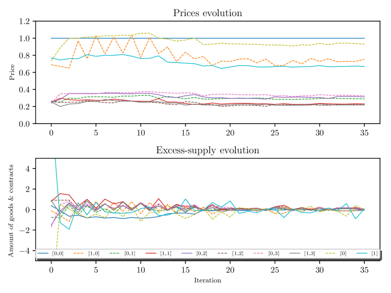
Figure 2: Augmented Walrasian iterations, evolution of prices ($\tilde{p}$, top) and Excess supply ${\rm ES}$ (bottom)

4.1.2 Comparison of Numerical Results

In this section, we will study the numerical results for the BDE example, comparing the original implementation on [4], the modify implementation by [24], an our approach.

Notice first that allocations $c$, contracts $z$ an contract prices $q$ are derived from the normalization of the prices $p$ reported on both papers, normalizing the first good up to 1, and solving the agent problem with our implementation. A summary of the different equilibrium is described on table 1

Table 1: Comparison: Equilibrium allocations, financial contracts, excess supply, and prices

	Ma[24, Ex1]				BDE[4, 5.1]				DW
c[i][l,s]	Ag[0]	Ag[1,2]	ES	p	Ag[0]	Ag[1,2]	ES	p	Ag[0]	Ag[1,2]	ES	p
[0,0]	0.600	1.690	0.019	1.0000	0.603	1.699	-0.001	1.0000	0.605	1.726	-0.058	1.0000
[1,0]	2.464	0.771	-0.006	0.7307	2.451	0.768	0.013	0.7375	2.406	0.762	0.069	0.7548
[0,1]	0.766	2.369	-0.003	0.2885	0.773	2.367	-0.007	0.2890	0.758	2.365	0.011	0.2887
[1,1]	2.981	1.024	-0.030	0.2224	2.965	1.010	0.016	0.2259	2.956	1.024	-0.004	0.2222
[0,2]	0.724	2.135	0.006	0.3057	0.716	2.149	-0.015	0.3056	0.744	2.109	0.038	0.3171
[1,2]	3.039	0.996	-0.031	0.2184	2.994	0.999	0.008	0.2193	3.094	0.975	-0.044	0.2286
[0,3]	0.680	1.903	0.014	0.3252	0.688	1.907	-0.002	0.3256	0.677	1.897	0.028	0.3272
[1,3]	3.100	0.965	-0.030	0.2138	3.112	0.958	-0.029	0.2159	3.105	0.966	-0.038	0.2141
z[i][j]	Ag[0]	Ag[1,2]	EC	q	Ag[0]	Ag[1,2]	EC	q	Ag[0]	Ag[1,2]	EC	q
[0]	-6.588	3.239	-0.110	0.9194	-6.247	3.210	0.173	0.9203	-6.304	3.162	0.020	0.9330
[1]	10.872	-5.348	0.177	0.6547	10.306	-5.267	-0.228	0.6611	10.481	-5.259	-0.037	0.6650

Rigorous metrics of comparison between the application of these algorithms are out of the scope of our exposition. Nevertheless, our implementation of the augmented Walrasian algorithm for this equilibrium problem performs robustly for several starting points. Moreover, as the underlying structure of the equilibrium problem solved incorporates the non-arbitrage condition, each iteration depicted in 2 provides a notion of stability. Additionally, no special attention has to be paid to intermediate steps where the market becomes incomplete or space spanned by the financial contracts at a particular price loss rank.

4.2 Two modifications to BDE example (4.1) by Schmedders [31]

Following the modifications introduced by Schmedders of the previous example, consider the following problems

4.2.1 Endowments variation [31, Ex.2,§6.2]

The first modification to Example 4.1, considers the same economy as before. Besides a substitution in the initial endowment of agent A,

$$e_{A}=\left(\begin{array}[]{ccccc}2.0&0.8&1.0&0.6\\ 2.0&2.4&3.0&1.8\end{array}\right)$$

the other parameters remains the same. Running this experiments, we found the equilibrium prices for the auxiliary problem is

$${\tilde{p}}^{*}=\left(\begin{array}[]{ccccc}1.0000&0.3230&0.2769&0.3928\\ 0.8013&0.2050&0.1640&0.1969\end{array}\right),$$

and using the transformation in 6, the equilibrium prices for the original economy are

$${p}^{*}=\left(\begin{array}[]{ccccc}1.0000&1.0000&1.0000&1.0000&\\ 0.8013&0.6347&0.5921&0.5013\end{array}\right),\quad q^{*}=\binom{0.9928}{0.5659},\quad r^{*}=0.73\%$$

Figure (3) depicts the iterations of the algorithm, and our method avoid the numerical instabilities that arise naturally from homotopy-type algorithms.

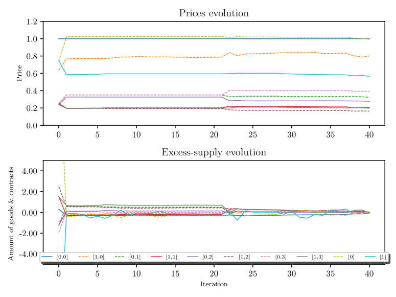
Figure 3: Example 4.2.1, evolution of prices ($\tilde{p}$, top) and Excess supply ${\rm ES}$ (bottom)

4.2.2 Homogeneous agents, no financial trade [31, Ex.3,§6.2]

This variation of the previous example, Example 4.1, considers only two agents, where the special feature is the constant total inital endowment $\sum_{i=1}^{\cal I}e^{i}_{l}(\xi)=3,\,\xi=0,\ldots,\Xi,\,l=0,1$. By symmetry, this economy should have equilibrium prices that are identical. Our results are similar to the ones found in the original paper, where this optimal prices are called bad prices. Figure (4) show the behavior of the augmented Walrasian, it is easy to see the asymptotic convergence to the equilibrium prices.

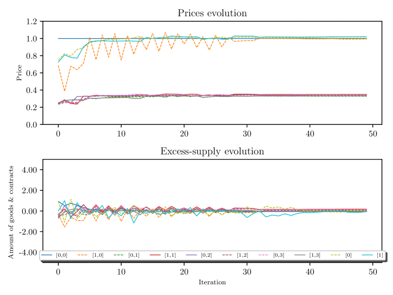
Figure 4: Example 4.2.2, evolution of prices ($\tilde{p}$, top) and Excess supply ${\rm ES}$ (bottom)

4.3 Heterogeneous agents, retention, and financial trade

In this example, we consider a bigger economy, $|{\cal I}|=5$ agents, $3$ possible scenarios on the second stage, $|L|=6$ commodities, and $|J|=5$ financial contracts. Agents’ utility functions are described by

$$U^{i}(c,w)=-\sum_{\xi=0}^{\Xi}\lambda_{\xi}^{i}\left(K-\prod_{l=1}^{L}c_{l,\xi}^{\alpha^{i}_{l,\xi}}-\rho\prod_{l=1}^{L}w_{l,\xi}^{\alpha^{i}_{l,\xi}}\right)^{2}$$

where $\xi=0$ represent the first-stage, and $\lambda$ is a factor that incorporates the probability distribution (in this example $\lambda_{\xi}^{i}=\left(1,\frac{1}{3},\frac{1}{3},\frac{1}{3}\right),\forall i,\xi)$. Additionally, consider the following agent parameters: $K=5.7$, $\rho=0.01$, and the utility coefficients $\alpha^{i}_{l,\xi}=\alpha^{i}_{l}$, for $\xi=0,\ldots,3$, and are given by

$\alpha^{i}_{l}$	$l=1$	$l=2$	$l=3$	$l=4$	$l=5$	$l=6$
$i=1$	0.25	0.25	0.17	0.17	0.08	0.08
$i=2$	0.25	0.25	0.17	0.17	0.08	0.08
$i=3$	0.17	0.17	0.25	0.25	0.08	0.08
$i=4$	0.17	0.17	0.25	0.25	0.08	0.08
$i=5$	0.08	0.08	0.08	0.08	0.5	0.17

and the initial endowments $e^{i}_{l,\xi}$ are taken as variation of a base vector $e^{i}_{l}$ and a stage-dependent random component, considering the following rule

$$e^{i}_{l,0}=e^{i}_{l},\quad\begin{cases}e^{i}_{l,1}=e^{i}_{l}+{\rm U}(0,0.1)\\ e^{i}_{l,2}=e^{i}_{l}\\ e^{i}_{l,3}=e^{i}_{l}-{\rm U}(0,0.1)\end{cases},$$

(where ${\rm U}(0,0.1)$ is a uniformly distributed random variable, supported in [0,0.1]) and the base vector is given by

$e^{i}_{l}$	$l=1$	$l=2$	$l=3$	$l=4$	$l=5$	$l=6$
$i=1$	1	4	2	2	3	1.5
$i=2$	4	1	2	2	1	1.5
$i=3$	2	1	4	3	1	1.5
$i=4$	2	4	1	3	1	1.5
$i=5$	2	2	2	2	2	2

In addition, the retention-related matrices $\{A(\xi)\}$ are given by identity matrices, and the financial market is formed by forward contracts, given by

$$D(0)=\mathbf{0}_{6\times 5},\quad D(\xi)=\left[\begin{array}[]{c}{\mathbf{I}}_{5}\\ \mathbf{0}_{1\times 5}\end{array}\right],\xi=1,\ldots,3,$$

i.e., no transaction costs are incurred when issuing a contract, and each contract represents a return of one unit of each first $J$ goods, for each possible scenarios of the second stage . Figure (5) depicts the trajectories of the prices (top) and excess supply (bottom) for each iteration of the augmented Walrasian algorithm. Note that this problem has a size of

$$\underbrace{I}_{\rm Agents}\cdot(\underbrace{2\cdot(L+1)\cdot(\Xi+1)}_{\rm Consumption+retention}+\underbrace{(J+1)}_{\rm Contracts})+\underbrace{(L+1)(\Xi+1)}_{\rm Prices-goods}+\underbrace{(J+1)}_{\rm Prices-contracts}=294$$

variables, considering the decisions made by each agent, in consumption, retention, and contracts, at each stage, and also the total amount of prices that needs to be determined.

Figure 5: Example 4.3, evolution of prices ($\tilde{p}$, top) and Excess supply ${\rm ES}$ (bottom)

The algorithm stopped after 54 iterations, with a tolerance of $\epsilon=0.1$, with the resulting vectors of prices

$$\{p_{l\xi}^{*}\}=\left[\begin{array}[]{cccc}1&1&1&1\\ 0.7421&0.9681&0.9003&0.8995\\ 0.7666&0.9913&0.9261&0.9334\\ 0.7355&0.9585&0.8947&0.8856\\ 1.0166&1.2086&1.1287&1.1326\\ 0.5706&0.7317&0.6928&0.7007\end{array}\right],\quad q^{*}=\left[\begin{array}[]{c}0.8035\\ 0.7401\\ 0.7625\\ 0.7323\\ 0.9280\end{array}\right]$$

References

- [1] K. J. Arrow and G. Debreu. Existence of an equilibrium for a competitive economy. Econometrica: Journal of the Econometric Society, pages 265–290, 1954.
- [2] J.-P. Aubin. Optima and equilibria: an introduction to nonlinear analysis, volume 140. Springer Science & Business Media, 2013.
- [3] P. Borges, C. Sagastizábal, and M. Solodov. Decomposition algorithms for some deterministic and two-stage stochastic single-leader multi-follower games. Computational Optimization and Applications, 78(3):675–704, 2021.
- [4] D. Brown, P. Demarzo, and C. Eaves. Computing Equilibria when Asset Markets are Incomplete. Econometrica, 64(1):1–27, 1996.
- [5] D. Brown and F. Kubler. Computational Aspects of General Equilibrium Theory: Refutable Theories of Value. Springer Berlin Heidelberg, 2008.
- [6] P. Demarzo and C. Eaves. Computing equilibria of GEI by relocalization on a Grassmann manifold. Journal of Mathematical Economics, 26(4):479–497, 1996.
- [7] J. Deride, A. Jofré, and R. J.-B. Wets. Solving deterministic and stochastic equilibrium problems via augmented Walrasian. Computational Economics, Sep 2017.
- [8] M. B. Donato, M. Milasi, and A. Villanacci. Incomplete financial markets model with nominal assets: Variational approach. Journal of Mathematical Analysis and Applications, 457(2):1353–1369, 2018. Special Issue on Convex Analysis and Optimization: New Trends in Theory and Applications.
- [9] C. Eaves, editor. Homotopy Methods and Global Convergence. Springer, 2011.
- [10] C. Eaves and K. Schmedders. General equilibrium models and homotopy methods. Journal of Economic Dynamics and Control, 23(9–10):1249–1279, 1999.
- [11] J. Garg, R. Mehta, M. Sohoni, and V. V. Vazirani. A complementary pivot algorithm for market equilibrium under separable, piecewise-linear concave utilities. SIAM Journal on Computing, 44(6):1820–1847, 2015.
- [12] J. Geanakoplos and W. Shafer. Solving systems of simultaneous equations in economics. Journal of Mathematical Economics, 19(1–2):69–93, 1990.
- [13] I. Gurobi Optimization. Gurobi Optimizer Reference Manual, 2014.
- [14] W. E. Hart, C. D. Laird, J.-P. Watson, D. L. Woodruff, G. A. Hackebeil, B. L. Nicholson, and J. D. Siirola. Pyomo–optimization modeling in python, volume 67. Springer Science & Business Media, second edition, 2017.
- [15] W. E. Hart, J.-P. Watson, and D. L. Woodruff. Pyomo: modeling and solving mathematical programs in python. Mathematical Programming Computation, 3(3):219–260, 2011.
- [16] J.-J. Herings and F. Kubler. Computing Equilibria in Finance Economies. Mathematics of Operations Research, 27(4):637–646, 2002.
- [17] J.-J. Herings and K. Schmedders. Computing Equilibria in Finance Economies with Incomplete Markets and Transaction Costs. Economic Theory, 27(3):493–512, 2006.
- [18] A. Jofré, R. Rockafellar, and R.-B. Wets. General economic equilibrium with financial markets and retainability. Economic Theory, 63(1):309–345, 2017.
- [19] A. Jofré and R.-B. Wets. Variational convergence of bivariate functions: Lopsided convergence. Mathemathical Programming B, 116:275–295, 2009.
- [20] A. Jofré and R.-B. Wets. Variational convergence of bifunctions: motivating applications. SIAM Journal on Optimization, 24(4):1952–1979, 2014.
- [21] A. Jofré and R. J.-B. Wets. Continuity properties of walras equilibrium points. Annals of Operations Research, 114(1-4):229–243, 2002.
- [22] A. Kirman. Elements of General Equilibrium Analysis. Wiley, 1998.
- [23] J. P. Luna, C. Sagastizábal, and M. Solodov. An approximation scheme for a class of risk-averse stochastic equilibrium problems. Mathematical Programming, 157(2):451–481, 2016.
- [24] W. Ma. A simple method for computing equilibria when asset markets are incomplete. Journal of Economic Dynamics and Control, 52:32–38, 2015.
- [25] M. Magill and M. Quinzii. Theory of Incomplete Markets, volume 1 of MIT Press Books. Mit press, 2002.
- [26] M. Milasi and D. Scopelliti. A stochastic variational approach to study economic equilibrium problems under uncertainty. Journal of Mathematical Analysis and Applications, 502(1):125243, 2021.
- [27] M. Powell. The BOBYQA algorithm for bound constrained optimization without derivatives. Cambridge NA Report NA2009/06, University of Cambridge, Cambridge, 2009.
- [28] R. Rockafellar and R.-B. Wets. Variational Analysis, volume 317 of Grundlehren der Mathematischen Wissenschafte. Springer Berlin Heidelberg, 2009.
- [29] R. Saigal. A homotopy for solving large, sparse and structured fixed point problems. Mathematics of Operations Research, 8:557–578, 1983.
- [30] H. Scarf and T. Hansen. The Computation of Economic Equilibria. Yale University Press, 1973.
- [31] K. Schmedders. Computing equilibria in the general equilibrium model with incomplete asset markets. Journal of Economic Dynamics and Control, 22(8–9):1375–1401, 1998.
- [32] S. Schommer. Computing equilibria in economies with incomplete markets, collateral and default penalties. Annals of Operations Research, 206(1):367–383, 2013.
- [33] A. Wächter and L. Biegler. On the implementation of an interior-point filter line-search algorithm for large-scale nonlinear programming. Mathematical programming, 106:25–57, 2006.
- [34] R.-B. Wets. Lipschitz continuity of inf-projections. Computational Optimization and Applications, 25(1-3):269–282, 2003.
- [35] D. C. Won. A new characterization of equilibrium in a multi-period finance economy: A computational viewpoint. Computational Economics, 53(1):367–396, 2019.
- [36] Y. Zhan and C. Dang. Determination of general equilibrium with incomplete markets and default penalties. Journal of Mathematical Economics, 92:49–59, 2021.
- [37] Y. Zhan and C. Dang. A smooth homotopy method for incomplete markets. Mathematical Programming, 190(1):585–613, 2021.