Answers to frequently asked questions about the pulsar timing array Hellings and Downs curve

Abstract

We answer frequently asked questions (FAQs) about the Hellings and Downs correlation curve—the “smoking-gun” signature that pulsar timing arrays (PTAs) have detected gravitational waves (GWs). Many of these questions arise from inadvertently applying intuition about the effects of GWs on LIGO-like detectors to the case of pulsar timing, where not all of that intuition applies. This is because Earth-based detectors, like LIGO and Virgo, have arms that are short (km scale) compared to the wavelengths of the GWs that they detect ($\approx 10^{2}$–$10^{4}$ km). In contrast, PTAs respond to GWs whose wavelengths (tens of light-years) are much shorter than their arms (a typical PTA pulsar is hundreds to thousands of light-years from Earth). To demonstrate this, we calculate the time delay induced by a passing GW along an Earth-pulsar baseline (a “one-arm, one-way” detector) and compare it in the “short-arm” (LIGO-like) and “long-arm” (PTA) limits. This provides qualitative and quantitative answers to many questions about the Hellings and Downs curve. The resulting FAQ sheet should help in understanding the “evidence for GWs” recently announced by several PTA collaborations.

,

• Jan 2024

Keywords: pulsar timing, gravitational waves, Hellings and Downs correlation

1 Introduction

Four pulsar timing array (PTA) collaborations recently announced the results of their latest searches for correlated low-frequency ($\sim\!10^{-9}~{}{\rm Hz}$) gravitational waves (GWs). The findings span the range from “weak evidence” for GWs for the (Australian) Parkes Pulsar Timing Array [1], “some evidence” for GWs for the Chinese Pulsar Timing Array [2], “evidence/marginal evidence” for GWs for the European Pulsar Timing Array [3], and “compelling evidence” for GWs for the North American Nanohertz Observatory for Gravitational Waves (NANOGrav) [4].

These observations can be challenging to understand, in part because the observed signal in the PTA band is unlike the short duration ($\sim\!0.25~{}{\rm s}$) GW “chirp” signal that LIGO observed on 14 Sep 2015, from the final inspiral and merger of two $\sim\!30M_{\odot}$ black holes. Instead of short (1 s) audio frequency (100 Hz) deterministic GW signals, PTAs search for persistent (signals with correlation times $\sim\!10^{3}$ yr which are in band for $\sim\!10^{6}$ yr), low-frequency (nHz) stochastic GW signals. These are too feeble to observe directly, but should produce correlated perturbations in the arrival times of pulses from an array of galactic millisecond pulsars.

Although the current PTA observations are not statistically significant enough to unambiguously claim a detection or to identify a source, a credible candidate is the superposition of GWs from hundreds of thousands of supermassive ($\sim\!10^{9}M_{\odot}$) black holes (SMBH) orbiting one another in the centers of merging galaxies. While any one of those binaries would produce a deterministic almost-constant-frequency signal, the incoherent sum of the GWs from many such sources creates a stochastic confusion noise: a “hubbub” of GWs.

PTAs search for correlations that are predicted to follow the so-called “Hellings and Downs” curve. This correlation curve is named after Ron Hellings and George Downs, who first derived it in 1983 [5]. The idea is that pulsars act as high-quality clocks, producing radio pulses that arrive at Earth with very predictable and regular arrival times. GWs induce slight perturbations in these arrival times, and these perturbations (called timing residuals) are correlated between different pulsars in a very specific fashion.

The Hellings and Downs curve is a plot of the expected or average correlation in the timing residuals from a pair of pulsars, as a function of their angular separation on the sky as seen from Earth. This curve is a prediction of general relativity (GR) for a gravitational-wave background (GWB) that is unpolarized and isotropic. More precisely, the Hellings and Downs curve is the expected value of the pulsar-pair correlations averaged over all pulsar pairs having the same angular separation and over GW sources having independent, random phases. Later, we will discuss several different interpretations for the curve, depending upon the type of averaging which is employed. Figure 1 shows how the timing residuals in NANOGrav’s 15-year dataset [4] appear to match this predicted Hellings and Downs curve.

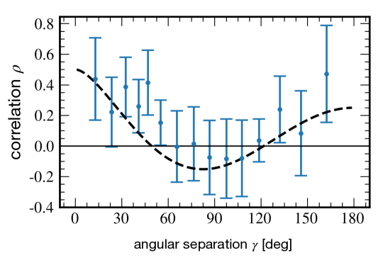
Figure 1: The spatial correlations observed in the pulsar timing residuals for the NANOGrav 15-year dataset [4] are shown in blue; the Hellings and Downs curve/prediction is shown in black. The blue points and error bars are optimally weighted averages of approximately 150 pulsar-pair correlations in each angular separation bin, which take into account covariances between the correlations induced by the GWB itself. (Reproduced from Figure 2c of [4].)

1.1 Frequently asked questions about the Hellings and Downs curve and the Hellings and Downs correlation

When giving talks about the recent PTA observations, the authors have repeatedly been asked certain questions about the properties of the Hellings and Downs correlation curve. The most common questions vary a bit, but can be summarized as:

1. Why is the Hellings and Downs curve in Figure 1 normalized to 1/2 at zero angular separation, but is normalized to $1/3$ in other papers? Does it matter?

2. Why does the Hellings and Downs curve have different values at $0^{\circ}$ and $180^{\circ}$ if the quadrupolar deformation of space produced by a passing GW affects two test masses $180^{\circ}$ apart in exactly the same way?

3. Why is the value of the Hellings and Downs curve for two pulsars separated by $180^{\circ}$ exactly half that for $0^{\circ}$ angular separation?

4. Why isn’t the most negative value of the Hellings and Downs curve at $90^{\circ}$?

5. Why is the Hellings and Downs curve frequency independent, whereas overlap functions for Earth-based interferometers are frequency dependent?

6. Does recovery of the Hellings and Downs curve imply that the GWB is isotropic?

7. In the distant future, when PTA observations are carried out with larger and more sensitive telescopes, more pulsars, and much longer observation periods, will we exactly recover the Hellings and Downs curve?

8. Assuming noise-free observations, are the fluctuations away from the expected Hellings and Downs curve due solely to the pulsar-term contributions to the timing residual response?

9. Why does the Hellings and Downs recovery plot shown in Figure 1 have error bars that are much larger than one would expect for the reported $3-4\sigma$ significance?

We believe that many of these questions arise because much of our intuition regarding the response of a detector to a passing GW was developed for Earth-based GW detectors such as LIGO and Virgo. Not all of it carries over to the case of PTAs. This is because the distance between the Earth and a pulsar (one “arm” of a PTA detector) is typically hundreds to thousands of times longer than the wavelengths ($\lambda\approx 10^{0}-10^{1}\,\text{light-years}$) of the GWs that PTAs are trying to detect. In contrast, Earth-based interferometers have km-long arms that are much shorter than the wavelengths ($\lambda\approx 10^{2}$–$10^{4}$ km) of the GWs that these detectors are sensitive to. In summary: PTA detectors operate in the “long-arm” (or short-wavelength) limit, whereas Earth-based laser interferometers operate in the “short-arm” (or long-wavelength) limit.

The goal of this paper is to provide qualitative and quantitative answers to the questions above, highlighting the differences between PTAs and LIGO-like detectors as appropriate.

Note that, as suggested by Q7, we make a distinction between (a) the Hellings and Downs curve, which is the black curve shown in Figure 1 and (b) the observed Hellings and Downs correlation, which might or might not follow this curve.

1.2 Outline

The remainder of this paper is organized as follows. There are two main parts: Part I consists of Sections 2 and 3, which provide the background information needed to derive the Hellings and Downs curve. This includes the calculation of the exact response of a single Earth-pulsar baseline to a passing GW, and two different averaging procedures used to obtain the expected correlation for pairs of Earth-pulsar baselines. Part II consists of Sections 4 and 5, which provide the answers to the FAQs listed above and a brief summary of the key points of the paper.

Readers who are already familiar with pulsar timing and the definition of the Hellings and Downs correlation could skip Sections 2 and 3 and jump directly to Section 4. However, we advise against that for two reasons: (i) In Sections 2.2 and 2.4, we compare the response of “long-arm” PTA pulsars to that of “short-arm” LIGO-like detectors, which we believe is the source of many of the misconceptions regarding the Hellings and Downs curve. (ii) Our discussion of pulsar averaging in Section 3.2 will be new to many, and the concepts introduced there are important for understanding what follows.

To make this article more accessible, we take a pedagogical approach. We avoid jargon, and either give “first-principles” explanations or provide pointers to papers containing these. We also suggest exercises for the reader. While no solutions are given, for the more involved exercises we point to published papers that contain these solutions.

From here forward, we use units in which the propagation speed $c$ of light and of GWs is equal to one. This means that both time and distance are measured in units of seconds or years as appropriate. More precisely, a distance is given by the time that it takes light to traverse that distance. For example, a meter stick is approximately 3 nanosec long, the LIGO detectors’ arms are about 10 microseconds long, the wavelengths of the GWs that PTAs are sensitive to are typically 10 years long, and typical pulsars are thousands of years from Earth.

We also adopt the Einstein summation convention for repeated spatial indices such as $i$ and $j$.

2 Single pulsar response

2.1 Single GW point source

We begin by describing the GWs emitted by a single very distant point source, and consider their effect on light (i.e., a radio pulse) propagating along an Earth-pulsar baseline. For example, imagine that the GWs are produced by an orbiting pair of SMBHs in the centers of two merging galaxies, $\sim\!10^{8}$ years from Earth. The SMBHs are separated by a distance of a few years, so from the perspective of Earth are a point source. For such a large distance from the source, the associated metric perturbations $h_{ij}(t,\vec{x})$ are solutions of the vacuum wave equation and are well approximated in the neighborhood of the Earth and pulsar by plane waves propagating in direction $\hat{\Omega}$, where $-\hat{\Omega}$ is the direction from Earth to the SMBH pair (see Figure 2).

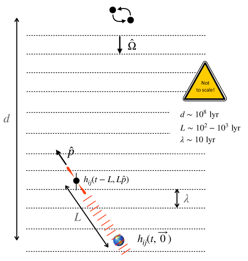
Figure 2: Geometry for the single pulsar analysis. The Earth is located at the origin of a rectangular coordinate system. The components $h_{ij}(t,\vec{x})$ of the metric perturbations are functions of time and of the Cartesian spatial coordinates $\vec{x}$. A single point source of GWs is located a distance $d$ from Earth in direction $-\hat{\Omega}$ on the sky. A galactic pulsar is located a distance $L$ from Earth in direction $\hat{p}$. The distances $\lambda$, $L$ and $d$ are related by $\lambda\ll L\ll d$, where $\lambda$ is the characteristic wavelength of the GWs that PTAs search for (of order 10 light-years).

In transverse-traceless-synchronous coordinates $(t,\vec{x})\equiv(t,x^{i})$, where $i=1,2,3$, we have

$$h_{ij}(t,\vec{x}) =\sum_{A=+,\times}h^{A}(t-\hat{\Omega}\cdot\vec{x})e^{A}_{ij}(\hat{\Omega})$$ (1a)

$$=\Re\left[h(t-\hat{\Omega}\cdot\vec{x})e^{*}_{ij}(\hat{\Omega})\right]\,,$$ (1b)

where

$$h(u)\equiv h^{+}(u)+ih^{\times}(u)\,,\quad e_{ij}(\hat{\Omega})\equiv e^{+}_{ij}(\hat{\Omega})+ie^{\times}_{ij}(\hat{\Omega})$$ (1b)

are complex combinations of the arbitrary real functions $h^{+}(u)$, $h^{\times}(u)$ and real polarization tensors $e^{+}_{ij}(\hat{\Omega})$, $e^{\times}_{ij}(\hat{\Omega})$ defined by

$$e^{+}_{ij}(\hat{\Omega})=\hat{m}_{i}\hat{m}_{j}-\hat{n}_{i}\hat{n}_{j}\,,$$ (1ca)

$$e^{\times}_{ij}(\hat{\Omega})=\hat{m}_{i}\hat{n}_{j}+\hat{n}_{i}\hat{m}_{j}\,.$$ (1cb)

Here, $\hat{m}$ and $\hat{n}$ are any two orthogonal unit vectors in the plane orthogonal to $\hat{\Omega}$. For stochastic background analyses, a common convention which we adopt here is

$$\hat{\Omega}\equiv-\hat{x}\,\sin\theta\cos\phi-\hat{y}\,\sin\theta\sin\phi-\hat{z}\,\cos\theta=-\hat{r}\,,$$ (1cda)

$$\hat{m}\equiv\hat{x}\,\sin\phi-\hat{y}\,\cos\phi=-\hat{\phi}\,,$$ (1cdb)

$$\hat{n}\equiv-\hat{x}\,\cos\theta\cos\phi-\hat{y}\,\cos\theta\sin\phi+\hat{z}\,\sin\theta=-\theta\,,$$ (1cdc)

where $\hat{r}$, $\hat{\theta}$, $\hat{\phi}$ are the standard spherical polar coordinate unit vectors, which are normal and tangent to the two-sphere. The vectors $\hat{\Omega}$, $\hat{m}$, and $\hat{n}$ are shown in Figure 3.

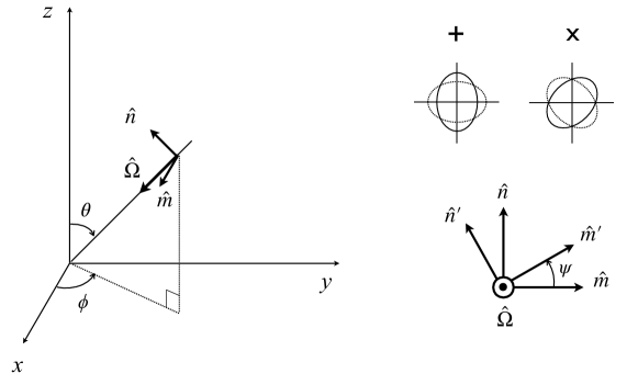
Figure 3: Left panel: Coordinate system and unit vectors used in the plane wave expansion. Right panel (top): two orthogonal polarizations of a GW. A circular ring of freely falling test particles is placed at rest in the plane orthogonal to the propagation direction $\hat{\Omega}$ of the wave. These are periodically deformed into ellipses, as space is “squeezed” and “stretched” by the passing of the GW. Right panel (bottom): an alternative choice of two orthogonal polarizations may be obtained by rotating $\hat{m}$ and $\hat{n}$ through angle $\psi$ to obtain new vectors $\hat{m}^{\prime}$ and $\hat{n}^{\prime}$.

The reader should be aware that in the literature there are two commonly-used mappings between the wave propagation direction and spherical polar coordinates $\theta,\phi$. In this work, as in [6, 7] the minus signs that appear in the mapping (1cda) mean that $\theta,\phi$ are the sky coordinates of the GW source. In the other papers that we cite [8, 9, 10, 11, 12], $\theta,\phi$ are the sky coordinates of the propagation direction; the GW source has antipodal coordinates $\pi-\theta,\phi+\pi$.

Note that for any GW propagation direction $\hat{\Omega}$, one can form an alternative orthonormal set of unit vectors by rotating $\hat{m}$ and $\hat{n}$ through an angle $\psi$ (called the polarization angle) in the plane orthogonal to $\hat{\Omega}$, as shown in the bottom right panel of Figure 3. We leave it as an exercise for the reader to show that such a rotation of $\hat{m}$ and $\hat{n}$ leads to a new set of polarization tensors

$$\left[\begin{array}[]{c}e^{\prime}{}^{+}_{ij}\\ e^{\prime}{}^{\times}_{ij}\end{array}\right]=\left[\begin{array}[]{cc}\phantom{-}\cos 2\psi&\sin 2\psi\\ -\sin 2\psi&\cos 2\psi\end{array}\right]\left[\begin{array}[]{c}e^{+}_{ij}\\ e^{\times}_{ij}\end{array}\right]\,,$$ (1cde)

or, equivalently,

$$e^{\prime}_{ij}(\hat{\Omega},\psi)=\exp(-i2\psi)\,e_{ij}(\hat{\Omega})\,.$$ (1cdf)

This change of polarization basis is a spin-two gauge transformation that leaves the metric perturbations $h_{ij}(t,\vec{x})$ unchanged. This is because the complex amplitude is multiplied by a phase which cancels that of (1cdf):

$$h^{\prime}(u)=\exp(-i2\psi)h(u),$$ (1cdg)

as can be seen from (1b). Note that this mixes $h_{+}(u)$ and $h_{\times}(u)$: $h^{\prime}_{+}$ and $h^{\prime}_{\times}$ are linear combinations of $h_{+}$ and $h_{\times}$. The gauge transformation is local, because if there are many sources with different $\hat{\Omega}$, then $\psi$ may be picked differently for each of these. The spin-two interpretation comes from quantum mechanics, where it indicates that the phase of the wave function rotates at twice the rate of the physical coordinate axes.

A particularly interesting case is the GWs emitted by a pair of SMBHs which are in a circular orbit with constant angular frequency, with an orbit that lies in the plane of the sky. This means that $\hat{\Omega}$ is parallel to the orbital angular momentum. The resulting GWs have components

$$h^{+}(t)=A\cos(2\pi f_{0}t+\phi_{0})\,,\quad h^{\times}(t)=A\sin(2\pi f_{0}t+\phi_{0})\,,$$ (1cdh)

where $A$ is a constant which is proportional to the inverse of the distance to the SMBHs. The complex waveform is

$$h(t)\equiv h^{+}(t)+ih^{\times}(t)=A\exp[i(2\pi f_{0}t+\phi_{0})]\,.$$ (1cdi)

Using (1b) and (1cdf), it follows that

$$h_{ij}(t,\vec{0})=A\,e^{\prime}{}^{+}_{ij}(\hat{\Omega},\psi(t))\,,\quad\psi(t)\equiv\frac{1}{2}\left[2\pi f_{0}t+\phi_{0}\right]\,,$$ (1cdj)

which describes a circularly polarized GW. The unit vectors $\hat{m}^{\prime}$ and $\hat{n}^{\prime}$ defining $e^{\prime}{}^{+}_{ij}(\hat{\Omega},\psi(t))$ rotate uniformly in the plane orthogonal to $\hat{\Omega}$ with angular velocity ${\rm d}\psi/{\rm d}t=\pi f_{0}$, which is the orbital angular velocity of the SMBH pair; the GW angular frequency is twice this.

For a circularly polarized GW source, the two linear polarization strain components are uncorrelated in time and have equal time-averaged squared values:

$$\overline{h^{+}(t)^{2}}=\overline{h^{\times}(t)^{2}}\,,\quad\overline{h^{+}(t)h^{\times}(t)}=0\,.$$ (1cdk)

Here, overbar denotes an average

$$\overline{F(t)}\equiv\frac{1}{T}\int_{-T/2}^{T/2}{\rm d}t\>F(t)$$ (1cdl)

over the observation time $T$, and we have assumed that $T$ is commensurate with the period of the wave, so that $f_{0}T=n$, where $n\neq 0$ is an integer.

Any gravitational-wave sources whose $+$ and $\times$ components satisfy (1cdk) are said to be unpolarized. At first, this seems to be a strange use of language, since it means that a circularly polarized source is “unpolarized”. A better way to think about it is this: an unpolarized source has no preferred polarization direction, as defined by the polarization angle $\psi$, in the plane perpendicular to $\hat{\Omega}$. So, according to this definition, a circularly polarized source is unpolarized, while a linearly polarized or elliptically polarized source is not unpolarized. The Hellings and Downs curve that we will discuss later is appropriate for a GWB made up of a superposition of unpolarized GW sources, or for a collection of polarized sources, provided that the collection does not define any preferred polarization angle.

2.2 Redshift response for a single Earth-pulsar baseline

As the GW passes the Earth-pulsar baseline, it affects the pulse arrival times. The change $\Delta T$ in the arrival time of the pulse as measured at Earth at time $t$ is obtained by projecting the metric perturbations along the direction to the pulsar $\hat{p}$, and then integrating that projection along the spacetime path of the pulse from emission at the pulsar to reception at Earth:

$$\Delta T(t)=\frac{1}{2}\hat{p}^{i}\hat{p}^{j}\int_{0}^{L}{\rm d}s\>h_{ij}(t(s),\vec{x}(s))\quad{\rm where}$$ (1cdma)

$$t(s)=t-(L-s)\,,\quad\vec{x}(s)=(L-s)\hat{p}\,.$$ (1cdmb)

Thus, the pulse “samples” the metric perturbations along its (null) path through spacetime. Note that we do not need to include any corrections to the straight-line path for the photon given above, as the metric perturbations are already first-order small and we can ignore all second- and higher-order terms in the calculation.

It turns out to be somewhat simpler mathematically to work instead with the Doppler shift in the pulse frequency induced by the GW. This Doppler or “redshift” response, which we will denote by $Z(t)$, is obtained by differentiating the timing residual response $\Delta T(t)$ with respect to time:

$$Z(t)\equiv\frac{{\rm d}\Delta T(t)}{{\rm d}t}=\frac{1}{2}\hat{p}^{i}\hat{p}^{j}\int_{0}^{L}{\rm d}s\>\frac{\partial h_{ij}}{\partial t}(t(s),\vec{x}(s))\,.$$ (1cdmn)

A redshift means an apparent lowering of the clock frequency corresponding to increase in the arrival period of the pulse, while a blueshift is the opposite. While “redshift” and “blueshift” are normally used in the context of visible light, they also apply to radio signals and even to the time delays between pulses from a pulsar, since relativistic effects are felt by all types of clocks and oscillators. (A detailed derivation of this equation in the context of temperature fluctuations in the cosmic microwave background was given by Sachs and Wolfe in [13]; see Eq. (39) in that paper. This was the first such occurrence of this equation that we are aware of.)

To perform the integration and differentiation that appear in (1cdmn), we first bring the time derivative inside the integral, differentiating the complex function $h(u(t,s))$ that enters the expression for $h_{ij}(t(s),\vec{x}(s))$, see (1b) and (1cdmb). Since

$$u(t,s)\equiv t(s)-\hat{\Omega}\cdot\vec{x}(s)=t-(L-s)(1+\hat{\Omega}\cdot\hat{p})\,,$$ (1cdmo)

it follows that

$$\frac{\partial h}{\partial t}=\frac{{\rm d}h}{{\rm d}u}\frac{\partial u}{\partial t}=\frac{{\rm d}h}{{\rm d}u}\,,\quad\frac{\partial h}{\partial s}=\frac{{\rm d}h}{{\rm d}u}\frac{\partial u}{\partial s}=(1+\hat{\Omega}\cdot\hat{p})\frac{{\rm d}h}{{\rm d}u}\,,$$ (1cdmp)

leading to

$$\frac{\partial h}{\partial t}=\frac{{\rm d}h}{{\rm d}u}=\frac{\partial h/\partial s}{\partial u/\partial s}=\frac{1}{(1+\hat{\Omega}\cdot\hat{p})}\frac{\partial h}{\partial s}\,.$$ (1cdmq)

The expression (1cdmn) can now be trivially integrated over $s$. Since the prefactor $1/(1+\hat{\Omega}\cdot\hat{p})$ does not depend on $s$, the integral is just the difference of $h(u(t,s))$ at the endpoints:

$$Z(t)=\frac{1}{2}\frac{{\hat{p}}^{i}{\hat{p}}^{j}}{1+{\hat{\Omega}}\cdot{\hat{p}}}\Bigl{[}h_{ij}\bigl{(}t,\vec{0}\bigr{)}-h_{ij}\bigl{(}t-L,L\hat{p}\bigr{)}\Bigr{]}\,.$$ (1cdmr)

This is the difference of the metric perturbations at the Earth at the instant when the pulse was received [$s=L\Rightarrow$ spacetime point $(t,\vec{0})$] and at the pulsar at the instant when the pulse was emitted [$s=0\Rightarrow$ spacetime point $(t-L,L\hat{p})$], projected onto the pulsar direction. The two terms are called the Earth term and pulsar term, respectively, and are explicitly shown in Figure 2.

This difference between the Earth and pulsar terms has a simple physical interpretation. As explained in [14, 15], the redshift (1cdmr) can be interpreted as a Doppler shift resulting from a relative velocity between the Earth and the pulsar, projected along the line of sight to the pulsar. This projected relative velocity is obtained by parallel-transporting the pulsar 4-velocity vector along the null geodesic traversed by the radio pulse. Via the Doppler effect, this nonzero relative velocity redshifts or blueshifts the photon frequency. If both source and receiver have the same projected velocity, then the Earth and pulsar term cancel, and the GW has no net effect on the photon redshift/pulsar timing residual.

We can also write the above expression for the redshift response $Z(t)$ as

$$Z(t)=\sum_{A}\Delta h^{A}(t,L\hat{p})F^{A}(\hat{\Omega})=\Re\left\{\Delta h(t,L\hat{p})F^{*}(\hat{\Omega})\right\}\,,$$ (1cdms)

where $\Delta h^{A}$ are the the Earth-to-pulsar differences in retarded waveforms:

$$\Delta h^{A}(t,L\hat{p})\equiv h^{A}(t)-h^{A}(t-L(1+\hat{\Omega}\cdot\hat{p}))\,,$$ (1cdmt)

and the $F^{A}$ are geometrical projection factors

$$F^{A}(\hat{\Omega})\equiv\frac{1}{2}\frac{{\hat{p}}^{i}{\hat{p}}^{j}}{1+{\hat{\Omega}}\cdot{\hat{p}}}e_{ij}^{A}(\hat{\Omega})\,,\quad A=+,\times\,.$$ (1cdmu)

The corresponding complex quantities $\Delta h(t,L\hat{p})$ and $F(\hat{\Omega})$ are defined by $\Delta h\equiv\Delta h^{+}+i\Delta h^{\times}$ and $F\equiv F^{+}+iF^{\times}$.

At first glance it appears that the geometrical projection factor $F^{A}(\hat{\Omega})$ diverges when $\hat{\Omega}=-\hat{p}$, since the denominator $1+\hat{\Omega}\cdot\hat{p}$ in (1cdmu) then equals zero. But the reader can easily verify that this zero in the denominator is canceled by a zero from the projection $\hat{p}^{i}\hat{p}^{j}e^{A}_{ij}(\hat{\Omega})$ when $\hat{p}$ is proportional to $\hat{\Omega}$ [take $\theta\to 0$ in (1cdmak)]. In fact, the redshift response $Z(t)$ vanishes for this case because the two functions in (1cdmt) are both evaluated at $t$ when $1+\hat{\Omega}\cdot\hat{p}=0$. This makes sense: a GW deforms space only in the plane transverse to its direction of propagation $\hat{\Omega}$. When $\hat{p}=-\hat{\Omega}$, the radio pulse does not feel these deformations.

2.3 Transfer functions and geometric projection factors

To visualize the response of a pulsar to a GW source, consider the simplest case: a circularly polarized GW source at sky position $-\hat{\Omega}$ radiating at a fixed GW frequency $f$. In a linear polarization basis the waveform is given by (1cdh), and in a circular ($\equiv$ complex) polarization basis it is given by (1cdi). Without loss of generality, the amplitude $A\geq 0$. From (1cdms), the redshift at Earth for a pulsar in direction $\hat{p}$ is

$$Z(t)=\Re\Bigl{(}A{\rm e}^{i(2\pi ft+\phi_{0})}\Bigl{[}1-{\rm e}^{-i2\pi fL(1+\hat{\Omega}\cdot\hat{p})}\Bigr{]}\Bigl{[}F^{+}(\hat{\Omega})-iF^{\times}(\hat{\Omega})\Bigr{]}\Bigr{)}\,.$$ (1cdmv)

The first quantity in square brackets is the redshift transfer function, which is the difference between the Earth term (unity) and the pulsar term (complex phase):

$${\cal T}(\alpha,\hat{\Omega}\cdot\hat{p})\equiv 1-e^{-i2\pi\alpha(1+\hat{\Omega}\cdot\hat{p})}\,.$$ (1cdmw)

The dimensionless parameter $\alpha\equiv fL=L/\lambda$ we have introduced is the ratio of the arm-length (i.e., the distance from Earth to pulsar) to the wavelength of the GW.

Return to the redshift in (1cdmv). Let $r\geq 0$ denote a real modulus and $\phi\in[0,2\pi)$ denote a real phase, so the redshift is

$$Z(t)=\Re\Bigl{(}r{\rm e}^{i(2\pi ft+\phi)}\Bigr{)}=r\cos(2\pi ft+\phi)\,.$$ (1cdmx)

The squared modulus can be read directly from (1cdmv), and is

$$r^{2}=A^{2}\left|1-{\rm e}^{-i2\pi fL(1+\hat{\Omega}\cdot\hat{p})}\right|^{2}\left[F^{+}(\hat{\Omega})^{2}+F^{\times}(\hat{\Omega})^{2}\right]\,.$$ (1cdmy)

Thus, the redshift oscillates sinusoidally with time according to (1cdmx), with an overall amplitude

$$r=A\bigl{|}{\cal T}(\alpha,\hat{\Omega}\cdot\hat{p})\bigr{|}|F(\Omega)|,$$ (1cdmz)

where

$$|F(\Omega)|=\sqrt{F^{+}(\hat{\Omega})^{2}+F^{\times}(\hat{\Omega})^{2}}$$ (1cdmaa)

is the quadrature combination of the pulsar’s responses to the two polarizations.

Is the redshift response for a source which is unpolarized [as defined by (1cdk)] described by the same quadrature combination? No, not unless the definition of “unpolarized” is generalized. This can be seen by computing the average squared redshift $\overline{Z^{2}(t)}$, where the overbar denotes the time average in (1cdl). This is proportional to $F^{+}(\hat{\Omega})^{2}+F^{\times}(\hat{\Omega})^{2}$ if

$$\overline{h^{+}(t)h^{+}(t+T)}=\overline{h^{\times}(t)h^{\times}(t+T)}\,,\text{ and }\overline{h^{+}(t)h^{\times}(t+T)}=0\,,$$ (1cdmab)

for an arbitrary value of $T$. If $h^{+}$ and $h^{\times}$ are ergodic processes, then these auto-correlation functions are related to the spectrum and cross spectrum of the two polarizations: the mean-squared redshift response will be described by the quadrature combination if $h^{+}$ and $h^{\times}$ have the same power spectrum and a vanishing cross spectrum.

The quadrature combination is also relevant for polarized sources, if there are no preferred orientations. To see this, first consider a single polarized source, defined by some complex waveform $h(u)=h^{+}(u)+ih^{\times}(u)$. From (1cdms), the redshift at Earth is $Z(t)=\Re[\Delta h(t,L\hat{p})F^{*}(\Omega)]$. How would that be changed if the axes which define the source’s polarization are rotated through an angle $\psi$ as shown in the bottom right panel of Figure 3? Because this does not change $\hat{\Omega}$ or the direction $\hat{p}$ to the pulsar, it only affects the redshift via $F$, which is modified because the complex polarization tensor appearing in $F$ is transformed according to (1cdf). Let $C_{R}$ and $C_{I}$ denote the real and imaginary parts of the complex quantity $C=C_{R}+iC_{I}=\Delta h(t,L\hat{p})F^{*}(\Omega)$. Then the redshift for this new source, with rotated polarization axes, is

$$Z(t)=\Re\left[C{\rm e}^{i2\psi}\right]=C_{R}\cos(2\psi)-C_{I}\sin(2\psi).$$ (1cdmac)

The average squared value of this quantity (uniformly averaged over all polarization orientations) is

$$Z^{2}_{\rm rms}(t)\equiv\frac{1}{2\pi}\int_{0}^{2\pi}\!\!\!\!\!{\rm d}\psi\,Z^{2}(t)=\frac{1}{2}\left(C_{R}^{2}+C_{I}^{2}\right)=\frac{1}{2}\left|C\right|^{2}.$$ (1cdmad)

Taking the square root of both sides, we find that the rms redshift is

$$Z_{\rm rms}=\frac{1}{\sqrt{2}}\bigl{|}h(t)-h(t-L(1+\hat{\Omega}\cdot\hat{p}))\bigr{|}\bigl{|}F(\Omega)\bigr{|}.$$ (1cdmae)

Thus, these quadrature combinations characterize the response of a PTA to an unpolarized source, or to a polarized source whose orientation is random.

The redshift (1cdms) is linear in the GW strain, and any GW strain can be decomposed into a sum of (left and right) circularly polarized plane waves of constant frequency. Hence, we can understand the response of a PTA to any GW signal by understanding the response of the PTA to a circularly polarized GW of constant frequency. In light of (1cdmv) it is convenient to define response functions

$$R^{A}(f,{\hat{\Omega}})\equiv\left[1-e^{-i2\pi fL(1+\hat{\Omega}\cdot\hat{p})}\right]F^{A}(\hat{\Omega})={\cal T}(\alpha,\hat{\Omega}\cdot\hat{p})F^{A}(\hat{\Omega})\,.$$ (1cdmaf)

The redshift transfer function ${\cal T}$ vanishes if the pulse from the pulsar traverses an integer number of cycles of GW-induced stretching and squeezing, because these integrate to give zero net timing delay. At fixed GW frequency $f$, this occurs for ${\rm int}[2\alpha]$ different incident directions, given by values of $\hat{\Omega}\cdot\hat{p}$ that satisfy

$$1+\hat{\Omega}\cdot\hat{p}=n/\alpha\quad{\rm where}\quad n=1,2,\dots,{\rm int}[2\alpha]\,.$$ (1cdmag)

The limit on $n$ arises because the left-hand side of (1cdmag) lies in the interval $[0,2]$. However, for a given GW direction (fixed $\hat{\Omega}\cdot\hat{p}$) there are an infinite number of $\alpha$ values (or frequencies) at which $\cal T$ vanishes. For normal incidence of the GW (i.e., $\hat{\Omega}\cdot\hat{p}=0$), these zeroes lie at $\alpha=n$ for $n=1,2,\dots$, as shown in Figure 4.

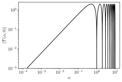
Figure 4: Modulus of the redshift transfer function ${\cal T}(\alpha,\hat{\Omega}\cdot\hat{p})$ for a normally incident ($\hat{\Omega}\cdot\hat{p}=0$) GW. It vanishes if the arm length is a multiple of the GW wavelength, $\alpha\equiv fL=n$ for $n=1,2,3,\dots$.

For a short-arm LIGO-like detector, the redshift transfer function (1cdmw) and the response function (1cdmaf) take simple forms. Expanding the exponential in (1cdmw) to first order in $\alpha\ll 1$ gives ${\cal T}\simeq i2\pi\alpha(1+\hat{\Omega}\cdot\hat{p})$, which implies (using $\alpha\equiv fL$)

$$R^{A}(f,\hat{\Omega})\simeq i2\pi fL\,G^{A}(\hat{\Omega})\,,\quad G^{A}(\hat{\Omega})\equiv\frac{1}{2}\hat{p}^{i}\hat{p}^{j}e_{ij}^{A}(\Omega)\,.$$ (1cdmah)

The geometrical projection factors $G^{A}(\hat{\Omega})$, where $A=+,\times$, are just the strain (i.e., $\Delta L/L$) response functions for a short one-arm, one-way LIGO-like detector. Note that this short-arm response function is symmetric under the interchange $\hat{p}\rightarrow-\hat{p}$, unlike $F^{A}(\hat{\Omega})$. This implies that if the distance from the Earth to a pulsar were much less than the GW wavelength, then the timing response of that Earth-pulsar baseline $\hat{p}$ would be exactly the same as that for a pulsar in the opposite sky direction, $-\hat{p}$. This symmetry can be seen graphically in the leftmost panels of Figures 5 and 6.

2.4 Visualizing the redshift response (antenna pattern functions)

It is helpful to visualize the response of a single Earth-pulsar baseline to an “unpolarized source” in the sense described above. From (1cdmz), for a unit-amplitude source ($A=1$) the relevant quantity is the polarization-averaged response function

$${\cal R}(f,\hat{\Omega})=\sqrt{|R^{+}(f,\hat{\Omega})|^{2}+|R^{\times}(f,\hat{\Omega})|^{2}}=|{\cal T}(\alpha,\hat{\Omega}\cdot\hat{p})|\,|F(\hat{\Omega})|\,,$$ (1cdmai)

with $\alpha\equiv fL$ as previously defined, and $|F(\hat{\Omega})|$ given by (1cdmaa). To examine the short-arm limit, we also define the quadrature combination

$$|G(\hat{\Omega})|\equiv\sqrt{G^{+}(\hat{\Omega})^{2}+G^{\times}(\hat{\Omega})^{2}}$$ (1cdmaj)

for the response in the short-arm limit, ignoring the prefactor $i2\pi fL$ relating $R^{A}(f,\hat{\Omega})$ and $G^{A}(\hat{\Omega})$, see (1cdmah).

Without loss of generality, consider a pulsar located in the $\hat{p}=\hat{z}$ direction

$$|F(\hat{\Omega})|=\frac{1}{2}(1+\cos\theta)\,,\quad|G(\hat{\Omega})|=\frac{1}{2}\sin^{2}\theta\,,\qquad$$ (1cdmak)

where $-\hat{\Omega}\cdot\hat{p}=\cos\theta$ is the cosine of the angle of the GW source relative to the pulsar direction. You will need to use (1ca), (1cb), (1cda), (1cdb), (1cdc), (1cdmah), and (1cdmu) to obtain these explicit expressions. As discussed above, $|F(\hat{\Omega})|$ is finite as $\theta\to 0$ and vanishes as $\theta\to\pi$, while $|G(\hat{\Omega})|$ vanishes at both $\theta=0,\pi$ (see the middle and left panels of Figure 6).

For fixed frequency $f$ and fixed distance $L$ to a pulsar, the shape of the polarization-averaged response function ${\cal R}(f,\hat{\Omega})$ depends only on the relative orientation of the GW propagation direction $\hat{\Omega}$ and the direction to the pulsar $\hat{p}$. The shape of ${\cal R}(f,\hat{\Omega})$ is often called an antenna pattern, because the magnitude of ${\cal R}$ is the “strength” of the response. Figure 5 shows plots of the antenna patterns ${\cal R}(f,\hat{\Omega})$ for a pulsar located in the $\hat{z}$ direction for different fixed values of $\alpha\equiv fL$. The left panel shows the antenna pattern in the “short-arm” LIGO-like limit, $\alpha\ll 1$, which is proportional to $\sin^{2}\theta$, as shown in (1cdmah) and (1cdmak). Note that the number of lobes of the antenna pattern increases as $\alpha$ increases, and that the overall magnitude of the antenna pattern function is proportional to $\alpha$ for $\alpha\ll 1$. Both of these behaviors are a consequence of the form of the redshift transfer function given in (1cdmw) and seen in Figure 4.

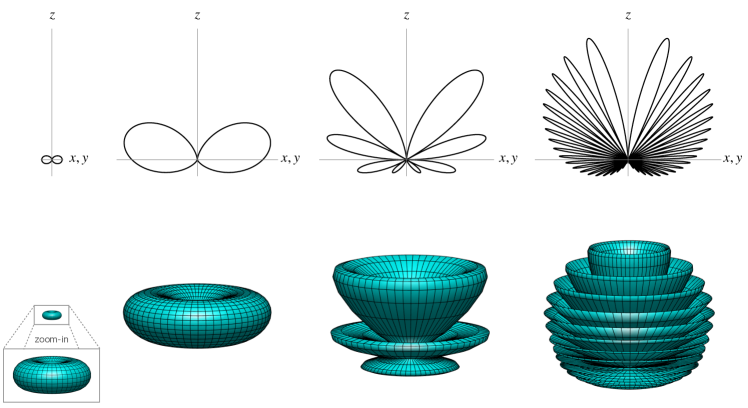
Figure 5: Antenna pattern functions ${\cal R}(f,\hat{\Omega})$ for the polarization-averaged redshift response of an Earth-pulsar baseline having $\hat{p}=\hat{z}$, evaluated for different fixed values of $\alpha\equiv fL$ (from left to right, $\alpha=0.05$, 0.5, 2, 10). The top row of plots are cross-sections: the antenna pattern functions are axially symmetric about the vertical $z$-axis. For example, the leftmost pattern resembles a doughnut with no hole, as shown in the bottom row of plots, which are the corresponding antenna patterns viewed from slightly above the $xy$ plane.

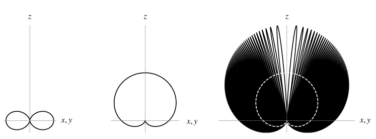
Figure 6: Antenna pattern functions for the polarization-averaged geometrical projection factors $|G(\hat{\Omega})|$ (left panel) and $|F(\hat{\Omega})|$ (middle panel). The right panel compares $|F(\hat{\Omega})|$ (white dashed curve) with the full polarization-averaged timing response function ${\cal R}(f,\hat{\Omega})$ for $fL=100$. All of these antenna pattern functions are axially symmetric around the vertical $z$-axis.

Recall that for most pulsars, $\alpha$ will be of order 100 or more, since the distance to typical pulsars is of order a kpc (so a few thousand light-years) or more, while the GW wavelengths are only of order tens of light-years. The rightmost panel of Figure 6 is a plot of ${\cal R}(f,\hat{\Omega})$ appropriate for the (semirealistic) case $\alpha=100$. Also plotted in this figure are the polarization-averaged antenna pattern functions for the geometrical projection factors $|G(\hat{\Omega})|$ (left panel) and $|F(\hat{\Omega})|$ (middle panel). Note that $|F(\hat{\Omega})|$ is half of the “envelope” of the full response function ${\cal R}(f,\hat{\Omega})$, illustrated by the dashed white curve in the rightmost panel plot.

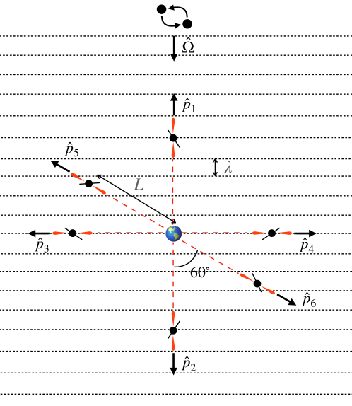
Figure 7: Six hypothetical pulsar locations relative to the Earth and a monochromatic GW propagating in direction $\hat{\Omega}$. All the pulsars lie in a plane, and are at distances $L=5\lambda$ with respect to the Earth, where $\lambda$ is the wavelength of the GW.

To end this section, we leave it as an exercise for the reader to calculate the values of the various antenna pattern functions $|G(\hat{\Omega})|$, $|F(\hat{\Omega})|$, and ${\cal R}(f,\hat{\Omega})$ for the different pulsar locations and GW shown in Figure 7. Similar to Figure 2, there is a single GW point source in direction $-\hat{\Omega}$ relative to Earth, sufficiently far away so that the waves are planar when they reach the vicinity of the Earth and the pulsars. We also assume that the GW is monochromatic with $fL\equiv L/\lambda=5$, where $\lambda$ is the GW wavelength and $L$ is the distance of the pulsars from Earth. The values of the various antenna patterns are given in Table 1.

Table 1: Values of the different geometrical and antenna pattern functions for the GW source and pulsar locations shown in Figure 7.

• Pulsar label	$a=1$	$a=2$	$a=3$	$a=4$	$a=5$	$a=6$
  Pulsar direction	$\hat{p}_{1}$	$\hat{p}_{2}$	$\hat{p}_{3}$	$\hat{p}_{4}$	$\hat{p}_{5}$	$\hat{p}_{6}$
  $|G_{a}(\hat{\Omega})|$	0	0	1/2	1/2	3/8	3/8
  $|F_{a}(\hat{\Omega})|$	1	0	1/2	1/2	3/4	1/4
  ${\cal R}_{a}(f,\hat{\Omega})$	0	0	0	0	3/2	1/2

2.5 The plane wave expansion

The plane wave expansion is widely used in the literature and provides a simple and precise way to write the pulsar response in the most general case of interest. If the PTA is far from the GW sources, then the GW metric perturbations in the PTA’s neighborhood may be written as a sum of plane waves

$$h_{ij}(t,\vec{x})=\sum_{A}\int df\int d\hat{\Omega}\,h_{A}(f,\hat{\Omega})e^{A}_{ij}(\hat{\Omega}){\rm e}^{i2\pi f(t-\hat{\Omega}\cdot\vec{x})}.$$ (1cdmal)

Here and elsewhere, frequency and time integrals are over the range $(-\infty,\infty)$, unless explicit limits are given.

One can see by inspection that $h_{ij}(t,\vec{x})$ satisfies the wave equation $(-\partial_{t}^{2}+\nabla^{2})h_{ij}=0$ and that it is transverse $\nabla_{i}h_{ij}=0$, traceless, and synchronous. The functions $h_{A}(f,\hat{\Omega})=h_{A}^{*}(-f,\hat{\Omega})$ are the complex Fourier amplitudes of the GW sources in direction $-\hat{\Omega}$ at frequency $f$. If there is a discrete set of sources, then the integral over $\hat{\Omega}$ may be replaced by a sum over those discrete sources, each of which has its own direction vector.

Substitute this plane wave expansion (1cdmal) into the formula for the redshift (1cdmn), differentiate with respect to $t$, and then integrate along the null ray coming from pulsar “a” as specified in (1cdmb). One obtains a compact formula for the redshift $Z_{a}(t)$ of an arbitrary pulsar in an arbitrary GW background:

$$Z_{a}(t) = \sum_{A}\int df\int d\hat{\Omega}\,R_{a}^{A}(f,{\hat{\Omega}})h_{A}(f,\hat{\Omega}){\rm e}^{i2\pi ft}\,.$$ (1cdmam)

The response function (1cdmaf) and the geometrical projection factor (1cdmu) carry the pulsar label “$a$”, and depend upon the pulsar’s distance $L_{a}$ and sky direction $\hat{p}_{a}$. They are given by

$$R_{a}^{A}(f,{\hat{\Omega}})\equiv\left[1-e^{-i2\pi fL_{a}(1+\hat{\Omega}\cdot\hat{p}_{a})}\right]F_{a}^{A}(\hat{\Omega})\,\ \Leftrightarrow\ R_{a}=R_{a}^{+}+iR_{a}^{\times}$$ (1cdman)

and

$$F_{a}^{A}(\hat{\Omega})\equiv\frac{1}{2}\frac{{\hat{p}_{a}}^{i}{\hat{p}_{a}}^{j}}{1+{\hat{\Omega}}\cdot{\hat{p}_{a}}}e_{ij}^{A}(\hat{\Omega})\,,\quad A=+,\times\,.$$ (1cdmao)

The response function elegantly incorporates the difference between the Earth term (unity) and the pulsar term (a complex phase).

3 Pulsar-pair correlations

Large amplitude GWs would be directly visible in the GW detector output. Indeed, in the early days of pulsar timing, upper limits were set on the amplitude of GWs by examining the timing residuals from single pulsars. The smallness of those residuals meant that the GW amplitudes could not have been too large.

However, the GWs predicted for typical background sources are too weak to be directly visible in the data; they cannot be separated from noise in the measurements or other physical effects. Fortunately, there is a way around this: look for a common GW signal by correlating the redshift measurements for two or more Earth-pulsar baselines for a PTA. With sufficient integration or averaging, one can “dig below the noise”. The same method (correlating signals from pairs of LIGO-like Earth-based detectors) is used to hunt for a stochastic background signal at audio frequencies [16, 10, 6].

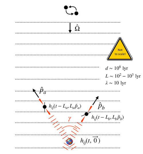
Figure 8: The geometry for the pulsar-pair correlation analysis is the same as in Figure 2, but with two Earth-pulsar baselines. The pulsars are labeled by $a$ and $b$ and are at distances $L_{a}$ and $L_{b}$ and directions $\hat{p}_{a}$ and $\hat{p}_{b}$ as seen from Earth. They are separated by angle $\gamma$ on the sky. As discussed in the text, we assume that the Earth-pulsar distances $L_{a}$, $L_{b}$ and the distance between the two pulsars $|L_{a}\hat{p}_{a}-L_{b}\hat{p}_{b}|$ are much greater than the correlation length of the relevant GWs. Consequently, the expression for the expected correlation only contains the Earth-term response functions $F_{a}(\hat{\Omega})$ and $F_{b}(\hat{\Omega})$ for the two pulsars.

3.1 Hellings and Downs correlation (source averaging)

To analyze these correlations, we extend the calculations of Sections 2.1, 2.2, and 2.3 to two Earth-pulsar baselines as shown in Figure 8. With respect to Earth, the two pulsars are at distances $L_{a}$ and $L_{b}$ and have sky directions $\hat{p}_{a}$ and $\hat{p}_{b}$.

As shown in Figure 8, we begin with a single GW point source, located very far away in direction $-\hat{\Omega}$ with respect to Earth. The correlation between noise-free redshift measurements $Z_{a}(t)$, $Z_{b}(t)$ for the two pulsars is given by the time-averaged product over the observation time

$$\rho_{ab}\equiv\overline{Z_{a}(t)Z_{b}(t)}\equiv\frac{1}{T}\int_{-T/2}^{T/2}{\rm d}t\>Z_{a}(t)Z_{b}(t)\,.$$ (1cdmap)

To study the properties of the correlation $\rho_{ab}$, particularly for an ensemble of GW sources, it is helpful to work in the frequency domain.

The frequency-domain representation for a single GW source is a special case of the general plane wave expansion (1cdmal), where the Fourier amplitudes vanish except for a single direction $\hat{\Omega}$. Alternatively, and equivalently, we can return to the formulation (1a) for a single source, and define Fourier amplitudes $\tilde{h}^{A}(f)$ for the source waveforms by

$$\tilde{h}^{A}(f)\equiv\int{\rm d}t\>e^{-i2\pi ft}\,h^{A}(t)\ \Leftrightarrow\ \tilde{h}(f)=\tilde{h}^{+}(f)+i\tilde{h}^{\times}(f)\,,$$ (1cdmaq)

where we give both the linear and complex polarization forms. The redshift of pulsar $a$ may then be written as

$$Z_{a}(t) =\int{\rm d}f\>e^{i2\pi ft}\sum_{A}\tilde{h}^{A}(f)R_{a}^{A}(f,\hat{\Omega})$$

$$=\Re\left[\int{\rm d}f\>e^{i2\pi ft}\tilde{h}(f)R_{a}^{*}(f,\hat{\Omega})\right].$$

The redshift of pulsar $b$ is given by the same expression as in (3.1), with $a\rightarrow b$.

The right-hand side of (1cdmap) contains 16 terms, because each pulsar redshift has contributions from two polarization components evaluated at both the Earth and pulsar, so there are four terms per pulsar. All of these terms contribute to $\rho_{ab}$ for a fixed set of GW sources and a fixed pair of pulsars.

However, for calculating the mean correlation for a pair of distinct Earth-pulsar baselines, only four terms survive, as described in detail in, e.g., [8, 9]. The argument that one uses to show this depends on the averaging procedure used to define the mean. The first form of averaging, employed by Hellings and Downs [5], keeps the pulsars fixed and averages the correlation $\rho_{ab}$ over GW source directions $\hat{\Omega}$, assuming that the sources are unpolarized and isotropic on the sky.

By performing the all-sky average for an unpolarized signal, the Earth-pulsar and pulsar-pulsar terms enter the expected correlation via integrals over $\hat{\Omega}$ of terms proportional to the auto-correlation function $C(\tau)$ of the GW signal evaluated at $\tau=\tau_{a}$, $\tau_{b}$, and $\tau_{a}-\tau_{b}$, where $\tau_{a}\equiv L_{a}(1+\hat{\Omega}\cdot\hat{p}_{a})$ and $\tau_{b}\equiv L_{b}(1+\hat{\Omega}\cdot\hat{p}_{b})$. As shown in [9], if we assume that the coherence length of the GW signal is short compared to $\tau_{a}$, $\tau_{b}$, and $|\tau_{a}-\tau_{b}|$, then these terms can be ignored relative to the Earth-Earth terms [see (C13) and Figures 8 and 9 in Appendix C of [9] for details]. However, for the correlation of a single pulsar with itself (i.e., $a=b$), it immediately follows that $\tau_{a}-\tau_{b}=0$. Thus, the auto-correlation function is evaluated at 0, and hence doubles the contribution of the Earth-Earth term for a stationary GW background.

The final result of this source-averaging approach, assuming that the coherence length is small as described above, is

$$\langle\rho_{ab}\rangle=h^{2}\mu_{\rm u}(\gamma)[1+\delta_{ab}]\,,$$ (1cdmas)

where

$$h^{2}\equiv\frac{1}{2}\left(\overline{(h^{+})^{2}+(h^{\times})^{2}}\right)=\frac{1}{2}\overline{|h|^{2}}\,,$$ (1cdmata)

$$\mu_{\rm u}(\gamma)\equiv\frac{1}{4\pi}\int{\rm d}\hat{\Omega}\>\sum_{A}F^{A}_{a}(\hat{\Omega})F^{A}_{b}(\hat{\Omega})=\frac{1}{4\pi}\int{\rm d}\hat{\Omega}\>F_{a}(\hat{\Omega})F^{*}_{b}(\hat{\Omega})\,.$$ (1cdmatb)

Here, $h^{2}$ is the squared GW strain and $\mu_{\rm u}(\gamma)$ is Hellings and Downs curve, which is the mean Hellings and Downs correlation for an unpolarized and isotropic GW background [5]. There is no contribution from the cross-polarization terms since $\overline{h^{+}h^{\times}}=0$ for unpolarized GW sources. The $\delta_{ab}$ term in (1cdmas) is needed to account for auto-correlations.

Simple symmetry arguments show that the integral in (1cdmatb) can depend only on the angle $\gamma$ between the lines of sight to the two pulsars. So, without loss of generality, we can place pulsar $a$ on the $z$-axis and pulsar $b$ in the $xz$-plane so that $\hat{p}_{a}=\hat{z}$ and $\hat{p}_{b}=\sin\gamma\,\hat{x}+\cos\gamma\,\hat{z}$. The polarization tensors needed to calculate $F^{A}_{a}(\hat{\Omega})$ and $F^{A}_{b}(\hat{\Omega})$ are defined by (1ca), (1cb), with $\hat{\Omega}$, $\hat{m}$, $\hat{n}$ given by (1cda), (1cdb), (1cdc). The integral can be evaluated analytically using contour integration, as detailed in [8, 9, 17], giving

$$\mu_{\rm u}(\gamma)=\frac{1}{3}-\frac{1}{6}\left(\frac{1-\cos\gamma}{2}\right)+\left(\frac{1-\cos\gamma}{2}\right)\ln\left(\frac{1-\cos\gamma}{2}\right)\,.$$ (1cdmatau)

This is an analytic expression for the Hellings and Downs curve for pulsar timing, expressed as a function of the angular separation between the directions to pairs of pulsars. A plot of this expected correlation is shown in the left panel of Figure 9, and also as the black dashed curve in Figure 1.

We leave it as an exercise for the reader to show that a similar calculation of the expected correlation for an array of “short-arm” LIGO-like detectors yields

$$\mu_{\rm u}(\gamma)\propto P_{2}(\cos\gamma)\,,$$ (1cdmatav)

where $P_{2}(x)$ is the $l=2$ Legendre polynomial. For this calculation, one needs to replace the response functions $R^{A}(f,\hat{\Omega})$ in (1cdmaf) with the short-arm limiting expressions (1cdmah). This substitution simplifies the integrand in (1cdmatb) to quadratics in $\sin\phi$ and $\cos\phi$ and quartics in $\cos\theta$. The short-arm expected correlation is plotted in the right panel of Figure 9. Since the short-arm function involves only the $l=2$ Legendre polynomial, it is an example of a purely quadrupolar correlation.

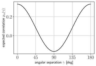
Figure 9: Left panel: Expected Hellings and Downs correlation for pairs of PTA pulsars. Right panel: Expected correlation for pairs of short-arm LIGO-like detectors, normalized with the same zero-angular-separation value of 1/3. Note that the zero-angular-separation value in the left panel corresponds to a pair of pulsars located close on the sky but at significantly different distances. If they are much closer than a GW wavelength, or if they are the same pulsar, then the correlation equals twice the zero-angular-separation value that is shown in this plot.

3.2 Pulsar averaging

The second form of averaging, originally proposed by Cornish and Sesana [18] and then further developed by the authors in [9, 19], is called pulsar averaging. Here, for a fixed set of GW sources, one averages the correlation $\rho_{ab}$ over all pulsar pairs separated by the same angle $\gamma$, assuming that one has access to a large number of pulsar pairs uniformly distributed on the sky. Pulsar averaging, like source averaging, eliminates the pulsar-pulsar and Earth-pulsar terms, provided the distances to pulsars in the same direction $\hat{p}$ are large compared to the GW wavelengths that PTAs are expected to detect. The result of pulsar averaging is a quantity

$$\Gamma(\gamma)\equiv\langle\rho_{ab}\rangle_{ab\in\gamma}\,,$$ (1cdmataw)

which depends only on the angular separation $\gamma$ between pulsars $\hat{p}_{a}$ and $\hat{p}_{b}$.

Pulsar averaging corresponds to observational practice. PTA collaborations monitor many pulsars distributed across the sky, so they can average together the correlations from all pulsar pairs lying in an angular separation bin centered on angle $\gamma$. As more pulsars are added to a PTA, the closer this “binned” pulsar averaging will get to ideal pulsar averaging, where one has access in principle to an infinite number of pulsar pairs uniformly distributed over the sky. In contrast, source averaging is not observationally possible, since we have access to only one Universe and its associated (fixed) collection of GW sources.

As shown in [9, 18], pulsar averaging yields the mean correlation (1cdmas) as the original Hellings and Downs source-averaging prescription for a single GW source:

$$\Gamma(\gamma)=h^{2}\mu_{\rm u}(\gamma)[1+\delta_{ab}]\,.$$ (1cdmatax)

In FAQ Q6, we demonstrate the mathematical equivalence of these two approaches for this simple model universe consisting of a single GW source in a random direction. But for multiple GW sources, the result of pulsar averaging is more complicated; it depends on the type of sources that contribute to the combined GW signal as described in detail in [9] and in the answer to FAQ Q7.

4 Answers to frequently asked questions

Given the above background information, we are now ready to answer the questions that we listed in Section 1.

 

• Why is the Hellings and Downs curve in Figure 1 normalized to 1/2 at zero angular separation, but is normalized to $1/3$ in Figure 9 and in other papers, e.g., [5, 9]? Does it matter?

Answer: This normalization difference is an overall scale. It is completely arbitrary and makes no difference: any physically observable quantity (for example, the expected time-averaged product of the timing residuals or redshift responses of two pulsars) is independent of this normalization.

The reason why $1/3$ and $1/2$ have appeared in the literature is historical. The Hellings and Downs curve was first computed as the average product of the redshift responses of two pulsars to a unit-amplitude GW source, averaged over the sphere of GW source directions as described in Section 3.1. This average introduces a factor of $1/4\pi$ in (1cdmatb). Later, the Hellings and Downs curve was reinterpreted as a correlation coefficient for the redshift response of two pulsars, responding to the same GW source. For this case, one wants the correlation coefficient to equal unity if the two pulsars are identical (i.e., $a=b$). Since the expected correlation for two identical pulsars is twice that for two distinct pulsars separated by $0^{\circ}$ [due to the $\delta_{ab}$ term in (1cdmas)], one needs $\mu_{\rm u}(0)=1/2$ for the correlation-coefficient interpretation. This means multiplying the right-hand sides of (1cdmatb) and (1cdmatau) by 3/2.

 

• Why does the Hellings and Downs curve have different values at $0^{\circ}$ and $180^{\circ}$ if the quadrupolar deformation of space produced by a passing GW affects two test masses $180^{\circ}$ apart in exactly the same way?

Answer: The Hellings and Downs curve has different values at $0^{\circ}$ and $180^{\circ}$ due to the different denominators $1+\hat{\Omega}\cdot\hat{p}_{1}$ and $1+\hat{\Omega}\cdot\hat{p}_{2}$, which appear in the antenna pattern functions $|F_{1}(\hat{\Omega})|$ and $|F_{2}(\hat{\Omega})|$ for the two pulsars. The two cases to consider for pairs of pulsars separated by $0^{\circ}$ and $180^{\circ}$ are $\hat{p}_{1}=\hat{p}_{2}=\hat{z}$ and $\hat{p}_{1}=-\hat{p}_{2}=\hat{z}$, respectively. This difference is illustrated graphically in the left panel of Figure 10, where we plot the integrand $F^{+}_{1}(\hat{\Omega})F^{+}_{2}(\hat{\Omega})+F^{\times}_{1}(\hat{\Omega})F^{\times}_{2}(\hat{\Omega})$ of the expected Hellings and Downs correlation for these two different cases. It is apparent from this plot that if the GWB consisted of waves that only came from directions perpendicular to the Earth-pulsar baselines (so, in the $xy$-plane of this plot), then the values of the Hellings and Downs correlation at $0^{\circ}$ and $180^{\circ}$ would be exactly the same. But since an isotropic GWB has equal contributions from GWs coming from all different directions on the sky, the Hellings and Downs correlation for the case $\hat{p}_{1}=\hat{p}_{2}$ will be larger than that for $\hat{p}_{1}=-\hat{p}_{2}$. Why these values differ by exactly a factor of two is the topic of the next question.

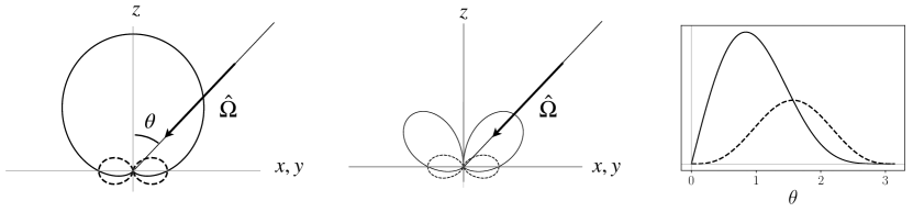
Figure 10: Integrands of the Hellings and Downs correlation curve for two pulsars separated by $0^{\circ}$ ($\hat{p}_{1}=\hat{p}_{2}=\hat{z}$, solid curve) and by $180^{\circ}$ ($\hat{p}_{1}=-\hat{p}_{2}=\hat{z}$, dashed curve). The first two panels are polar plots, which are axially symmetric about the $z$-axis. The left plot shows $F_{1}^{+}(\hat{\Omega})F_{2}^{+}(\hat{\Omega})+F_{1}^{\times}(\hat{\Omega})F_{2}^{\times}(\hat{\Omega})$ for the two different choices of $\hat{p}_{1}$ and $\hat{p}_{2}$. The polar plots in the middle panel include an additional factor of $\sin\theta$, which arises when integrating over $\theta$. The right panel is the same as the middle panel, but plotted as a function of $\theta$. The area under the solid curve is twice the area under the dashed curve.

 

• Why is the value of the Hellings and Downs curve for two pulsars separated by $180^{\circ}$ exactly half that for $0^{\circ}$ angular separation?

Answer: To prove this, start with (1cdmatb) for the expected Hellings and Downs correlation and (1cdmu) for the Earth-term-only response functions $F^{A}(\hat{\Omega})$. Taking the two pulsars to point in the same direction ($\hat{p}_{1}=\hat{p}_{2}=\hat{z}$), we have

$$\sum_{A}F_{1}^{A}(\hat{\Omega})F_{2}^{A}(\hat{\Omega})=\frac{1}{4}(1+\cos\theta)^{2}=\frac{1}{4}(1+u)^{2}\,,$$ (1cdmatay)

where $u=\cos\theta$. Having them point in opposite directions ($\hat{p}_{1}=-\hat{p}_{2}=\hat{z}$) leads to

$$\sum_{A}F_{1}^{A}(\hat{\Omega})F_{2}^{A}(\hat{\Omega})=\frac{1}{4}(1-\cos^{2}\theta)=\frac{1}{4}(1-u^{2})\,.$$ (1cdmataz)

These functions are plotted in Figure 10, where $\theta$ is the usual polar angle measured with respect to the $z$-axis. [Note: the comment following (1cdc) explains why $u=\cos\theta$ has the opposite sign in some of the literature, for example in Eq. D10 of [9].]

The overlap function is the average of this quantity over the sphere. From the three panel plots in Figure 10, we see that when the two pulsars both point in the $\hat{z}$ direction, the majority of support for the overlap function comes from sky directions $\hat{n}=-\hat{\Omega}$ having $z>0$. When the two pulsars point in opposite directions, $\hat{p}_{1}=-\hat{p}_{2}=\hat{z}$, the overlap function has equal contributions from $z>0$ and $z<0$. These contributions are only slightly larger than those for $\hat{p}_{1}=\hat{p}_{2}$ for $z<0$, but much smaller for $z>0$.

Visual inspection of the areas under the two curves shown in the rightmost panel of Figure 10 shows why the value of the HD curve for two pulsars separated by $0^{\circ}$ is twice as large as that for two pulsars separated by $180^{\circ}$. Indeed, averaging these quantities over the sphere gives

$$\mu_{\rm u}(0^{\circ})=\frac{1}{3}\quad(\hat{p}_{1}=\hat{p}_{2}=\hat{z})\,,\quad\mu_{\rm u}(180^{\circ})=\frac{1}{6}\quad(\hat{p}_{1}=-\hat{p}_{2}=\hat{z})\,.$$ (1cdmatba)

These values are easy to check, since the average of a function $Q(u)$ over the sphere is $(1/4\pi)\int d\hat{\Omega}\>Q(\cos\theta)=(1/4\pi)\int_{0}^{2\pi}{\rm d}\phi\int_{0}^{\pi}{\rm d}\theta\>\sin\theta\,Q(\cos\theta)=(1/2)\int_{-1}^{1}{\rm d}u\>Q(u)$. The integrals of (1cdmatay) and (1cdmataz) with respect to $u$ are trivial.

 

• Why isn’t the most negative value of the Hellings and Downs curve at $90^{\circ}$?

Answer: Again, this is because the Earth-term-only response functions $F^{A}(\hat{\Omega})$ given in (1cdmu) are not symmetric under $\hat{p}\rightarrow-\hat{p}$. If the Hellings and Downs correlation were purely quadrupolar, then its most negative value would be exactly at $90^{\circ}$, as it is for the case of an array of short-arm LIGO-like detectors (see the right panel of Figure 9). If it had only even multipoles (no odd-$l$ terms) then it would be reflection symmetric about $90^{\circ}$ but might not have its minimum there.

Although the dominant contribution to the Hellings and Downs curve is the quadrupole pattern $P_{2}(\cos\gamma)$, there are nonzero contributions from all higher order $l$-modes as well. We leave it as an exercise for the reader to show that

$$\mu_{\rm u}(\gamma)=\sum_{l=2}^{\infty}(2\ell+1)c_{l}P_{l}(\cos\gamma)\,,\quad{\rm where}$$ (1cdmatbb)

$$c_{l}=[(l+2)(l+1)l(l-1)]^{-1}\,.$$ (1cdmatbc)

To obtain this result, one needs to use (a) the orthogonality property

$$\int_{-1}^{1}{\rm d}x\>P_{l}(x)P_{l^{\prime}}(x)=\frac{2}{2l+1}\delta_{ll^{\prime}}$$ (1cdmatbd)

of the Legendre polynomials, where $x\equiv\cos\gamma$, (b) Rodrigues’ Formula for Legendre polynomials, and (c) integration by parts. See equations (97)–(105) in [12] for a step-by-step derivation of (1cdmatbb) and (1cdmatbc).

Figure 11 compares approximate versions of the Hellings and Downs curve, terminating the sum at different maximum values $l_{\rm max}=2,3,4,5$. Since the $c_{l}$’s in (1cdmatbc) fall off like $1/l^{4}$, only a few values of $l$ are needed to get a very good approximation.

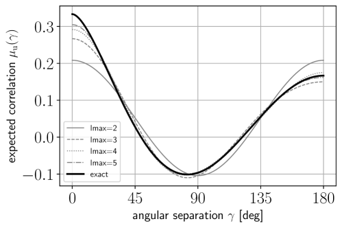
Figure 11: Approximations to the Hellings and Downs curve (solid black) obtained by terminating the sum in (1cdmatbc) with two to five Legendre polynomials (grey curves).

 

• Why is the Hellings and Downs curve/correlation frequency independent, whereas overlap functions for Earth-based interferometers are frequency dependent, for example, as shown in Figure 2 of Ref. [10]?

Answer: The expected Hellings and Downs correlation for a pair of pulsars $a$ and $b$ does not depend on frequency since the frequency dependence of the redshift response functions $R^{A}_{a}(f,\hat{\Omega})$ and $R^{A}_{b}(f,\hat{\Omega})$ given in (1cdmaf) enters only via the pulsar terms $e^{-i2\pi fL_{a}(1+\hat{\Omega}\cdot\hat{p}_{a})}$ and $e^{-i2\pi fL_{b}(1+\hat{\Omega}\cdot\hat{p}_{b})}$. These terms drop out when calculating the expected correlation of $Z_{a}(t)$ and $Z_{b}(t)$, as described in Section 3.1.

However, for a pair of Earth-based interferometers, each of which has two perpendicular equal-length arms, the corresponding response functions have the form [20]:

$$R_{a}^{A}(f,\hat{\Omega})=F^{A}(\hat{\Omega})e^{-i2\pi f\hat{\Omega}\cdot\vec{r}_{a}}\,,$$ (1cdmatbea)

$$F_{a}^{A}(\hat{\Omega})\equiv\frac{1}{2}(\hat{X}_{a}^{i}\hat{X}_{a}^{j}-\hat{Y}_{a}^{i}\hat{Y}_{a}^{j})e^{A}_{ij}(\hat{\Omega})\,,\quad A=+,\times\,,$$ (1cdmatbeb)

where $\hat{X}_{a}$, $\hat{Y}_{a}$ are unit vectors pointing along the two arms of the interferometer, and $\vec{r}_{a}$ is the position vector of the interferometer’s central station. (Similar equations hold for the second interferometer with $a$ replaced by $b$.) When forming the expected correlation, we need to evaluate the integral

$$\frac{1}{4\pi}\int{\rm d}\hat{\Omega}\>\sum_{A}F^{A}_{a}(\hat{\Omega})F^{A}_{b}(\hat{\Omega})\,e^{-i2\pi f\hat{\Omega}\cdot(\vec{r}_{a}-\vec{r}_{b})}\,.$$ (1cdmatbebf)

Now, for two interferometers on Earth, the distance $D_{ab}\equiv|\vec{r}_{a}-\vec{r}_{b}|$ between the central stations is comparable to the wavelength $\lambda\equiv 1/f$ (hundreds to thousands of km) of the GWs that these instruments detect. Hence, this exponential factor cannot be approximated by unity. (As discussed in Sec. 1, for PTAs, the timing residuals are determined at the same point, the SSB, for all pulsars and all telescopes. So for PTAs, $\vec{r}_{a}-\vec{r}_{b}=\vec{0}$, implying that $e^{-i2\pi f\hat{\Omega}\cdot(\vec{r}_{a}-\vec{r}_{b})}=1$.) Thus, while individual Earth-based interferometers operate in the short-arm limit $L\ll\lambda$, it is not also the case that $D_{ab}\ll\lambda$, but rather that $\lambda\lesssim D_{ab}$. Since the frequency dependence for Earth-based interferometers is tied to the detector locations, it cannot be factored out of the correlation as a detector-independent function of frequency.

 

• Does recovery of the Hellings and Downs curve from observed pulsar-pair correlations imply that the GWB is isotropic?

Answer: No. The Hellings and Downs curve is a robust prediction for the correlation produced by any (small or large) set of noninterfering GW sources, provided pulsar averaging is carried out using many pairs of pulsars uniformly distributed over the sky. It is independent of the angular distribution of the GW sources on the sky. This result was first demonstrated for the special case of GWs produced by a single black-hole binary in [18]. It was then extended to an arbitrary set of noninterfering sources in [9] (see also FAQ Q7 below), which further exploited pulsar averaging. For interfering sources, we do not expect to recover exactly the Hellings and Downs curve (see [9] and FAQ Q7 below).

As discussed in Section 3.1, the original/traditional approach to compute the expected Hellings and Downs correlation is to take a single fixed pair of pulsars, and then to average their correlation over GW propagation directions $\hat{\Omega}$, assuming that the sources are unpolarized and isotropic on the sky [5]. In references [18] and [9], somewhat involved calculations were done to show the equivalence of pulsar averaging and source averaging for the case of a single GW source, see (1cdmatax).

Happily, one can show the equivalence of these two approaches without any calculation. Here, we show that pulsar averaging is equivalent to GW-source averaging, with a purely geometric argument, using a series of three Euler-angle rotations. At first, this appears to require adding something to the traditional source-averaging calculation: in addition to averaging over the GW propagation directions $\hat{\Omega}=\hat{\Omega}(\theta,\phi)$ one must also average over the polarization angle $\psi$. In fact, while often overlooked, this is also required by the traditional calculation: it gives rise to the quadrature sum. It is overlooked because the original [5] calculation obscures this point by not giving enough detail. To obtain that result, one must assign a polarization direction or angle to each source, and also average over that, for example, as in the calculation starting from (1cdmac). Hence, even in the traditional GW-source averaging approach, the averages must be calculated with respect to three angles, not just two.

To see the equivalence purely from geometry, start with the averaging over GW source directions. As is often done, without loss of generality, put $\hat{p}_{1}$ along the $z$-axis and $\hat{p}_{2}$ in the $xz$-plane, so that $\hat{p}_{2}=\sin\gamma\,\hat{x}+\cos\gamma\,\hat{z}$. In contrast, pulsar averaging is carried out with respect to the angular coordinates of $\hat{p}_{1}$ (polar coordinate $\theta$, azimuthal coordinate $\psi$) and those of $\hat{p}_{2}$ (which lies on a cone about $\hat{p}_{1}$ with fixed half-opening angle $\gamma$, with its location on the cone parameterized by $\phi\in[0,2\pi)$). See Figure 12 and compare with Figure 5 of [9].

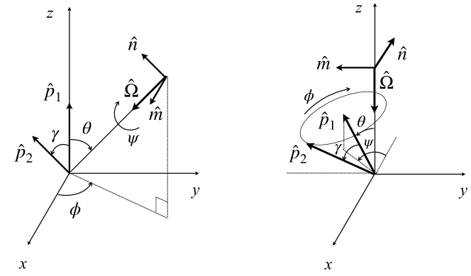
Figure 12: GW source averaging (left panel) and pulsar averaging (right panel) are equivalent, as can be seen by carrying out a series of rotations.

The sequence of rotations needed to go from source averaging to pulsar averaging is as follows: first rotate by $-\phi$ about the $z$-axis, which moves the GW propagation direction $\hat{\Omega}$ into the $xz$-plane and $\hat{p}_{2}$ around a cone with central axis $\hat{p}_{1}$ through angle $\phi$. Then rotate by $-\theta$ around the $y$ axis, which puts $\hat{\Omega}$ along $-\hat{z}$, and makes $\hat{p}_{1}$ have polar angle $\theta$. Finally, rotate around $\hat{\Omega}$ (which now points in the $-\hat{z}$ direction) by $-\psi$, which becomes the azimuthal angle for $\hat{p}_{1}$ (with respect to the $-x$-axis).

In practice, we do not have an infinite number of pulsar pairs separated by the angle $\gamma$. So, to do pulsar averaging, one divides the $N_{\rm pul}(N_{\rm pul}-1)/2$ interpulsar correlations into a smaller number $N_{\rm bins}$ of angular separation bins. This form of pulsar averaging is always used when attempting to recover or reconstruct the Hellings and Downs curve based on observed interpulsar correlations. For example, for the NANOGrav 15-year analysis shown in Figure 1, $N_{\rm pul}=67$ and $N_{\rm bins}=15$, which implies that the estimated correlation value in each angular separation bin involved averaging the correlations of approximately 150 pulsar pairs.

 

• In the distant future, when PTA observations are carried out with larger and more sensitive telescopes, more pulsars, and much longer observation periods, will we exactly recover the Hellings and Downs curve?

Answer: As we shall show below, this would be the case if the GWB were produced by a set of discrete noninterfering sources [9, 21]. But it is much more likely that our Universe contains many GW sources radiating at frequencies that are close enough together that they cannot be resolved individually over the time span of the PTA experiments (say, tens to hundreds of years). This means that the GWB is produced by a sum of interfering sources. An example of such a GWB is the “confusion noise” created by a set of sources randomly distributed on the sky, emitting monochromatic GWs with random phases, but occupying the same frequency bin [11]. In this case, pulsar-averaged noise-free measurements over an infinite number of pulsar pairs with the same angular separation do not give exactly the Hellings and Downs curve.

If we have an infinite collection of universes, each of which has GW sources having independent random phases, and we were also able to average the correlation over all of those universes (called an “ensemble average”), then we would get exactly the Hellings and Downs curve. But in any given universe, we would find something different from Hellings and Downs. The (mean squared) difference between what would be observed in any given universe, and the (unobservable) average over many universes, is called the cosmic variance.

It is easy to see how the cosmic variance arises from interference between different GW sources. Consider a universe which contains $N$ point sources of GWs, which we label $n=1,\dots,N$. These GW sources are located far from the neighborhood containing the Earth and the PTA pulsars. The GW sources have sky locations $-\hat{\Omega}_{n}$, and the $n$’th source produces a complex strain at Earth $h_{ij}(t)=\Re[h_{n}(t)e^{*}_{ij}(\hat{\Omega}_{n})]$, where the complex waveform is $h_{n}(t)=h_{n}^{+}(t)+ih_{n}^{+}(t)$. Since the PTA is far from the sources, these GW strains are small, so the total strain at Earth can be obtained by summing them. The redshift of pulsar $a$ is then obtained by summing (1cdms) to obtain

$$Z_{a}(t) =\Re\left[\sum_{n=1}^{N}h_{n}(t)F^{*}_{a}(\hat{\Omega}_{n})\right]$$ (1cdmatbebga)

$$=\frac{1}{2}\sum_{n}\Bigl{[}h_{n}(t)F^{*}_{a}(\hat{\Omega}_{n})+h^{*}_{n}(t)F_{a}(\hat{\Omega}_{n})\Bigr{]}\,,$$ (1cdmatbebgb)

where $F_{a}(\hat{\Omega})\equiv F_{a}^{+}(\hat{\Omega})+iF_{a}^{\times}(\hat{\Omega})$ are the complex antenna patterns, and we adopt the convention that sums over $n$ and $m$ are from $1,\cdots,N$ unless otherwise indicated. A similar expression holds for pulsar $b$. We assume that the pulsars $a$ and $b$ are distinct and are separated from one another by many GW wavelengths, and therefore have neglected the pulsar terms for the reasons discussed earlier. (We work with complex quantities because it simplifies some of the following.)

The correlation between the redshifts of the two pulsars is the time-averaged product $\rho_{ab}\equiv\overline{Z_{a}(t)Z_{b}(t)}$, which evaluates to

$$\hskip 25.29494pt\rho_{ab}=\frac{1}{4}\sum_{n}\sum_{m}\Bigl{[}\,\overline{h_{n}h_{m}^{*}}F^{*}_{a}(\hat{\Omega}_{n})F_{b}(\hat{\Omega}_{m})+\overline{h^{*}_{n}h_{m}}F_{a}(\hat{\Omega}_{n})F^{*}_{b}(\hat{\Omega}_{m})$$

$$\hskip 46.97505pt+\overline{h_{n}h_{m}}F^{*}_{a}(\hat{\Omega}_{n})F^{*}_{b}(\hat{\Omega}_{m})+\overline{h^{*}_{n}h^{*}_{m}}F_{a}(\hat{\Omega}_{n})F_{b}(\hat{\Omega}_{m})\Bigr{]}\,.$$ (1cdmatbebgbh)

To make the expression more compact, we do not explicitly show the time dependence of the quantities being time-averaged.

Next, we consider the pulsar average of (1cdmatbebgbh), which is obtained by averaging the correlation over all pulsar pairs $ab$ separated by angle $\gamma$. As discussed briefly in Sec. 3.2, and in more detail in [19], this corresponds closely to experimental practice: PTA experiments “reconstruct” the angular dependence of the Hellings and Downs correlation via a pulsar averaging procedure. Also, note that we dropped the pulsar terms from (1cdmatbebga). Had we included them, they would have been eliminated by this pulsar averaging step, as shown in Sec. IV of [9].

Consider first the case where there is no interference between GW sources, for example, because the sources are radiating GWs at different frequencies. This means that all the time averages $\overline{h_{n}h_{m}}$ and $\overline{h_{n}h^{*}_{m}}$ vanish if $n$ is different than $m$. Thus, in this no-interference case, the double sum reduces to a single sum:

$$\hskip 25.29494pt\rho_{ab}=\frac{1}{4}\sum_{n}\Big{[}\,\left(F^{*}_{a}(\hat{\Omega}_{n})F_{b}(\hat{\Omega}_{n})+F_{a}(\hat{\Omega}_{n})F^{*}_{b}(\hat{\Omega}_{n})\right)\overline{|h_{n}|^{2}}$$

$$\hskip 119.24506pt+2\Re\left(F^{*}_{a}(\hat{\Omega}_{n})F^{*}_{b}(\hat{\Omega}_{n})\,\overline{h^{2}_{n}}\right)\Big{]}.$$ (1cdmatbebgbi)

We now pulsar-average the correlation (1cdmatbebgbi). The only dependence on $a$ and $b$ in (1cdmatbebgbi) is via the antenna pattern functions. As explained in Q6 and Figure 12, the pulsar average of $F_{a}(\hat{\Omega}_{n})F^{*}_{b}(\hat{\Omega}_{n})$ is independent of the source direction $\hat{\Omega}_{n}$ and gives exactly the Hellings and Downs curve $\mu_{\rm u}(\gamma)$. The pulsar average of $F_{a}(\hat{\Omega}_{n})F_{b}(\hat{\Omega}_{n})$ vanishes. Hence, the pulsar average of (1cdmatbebgbi) gives

$$\langle\rho_{ab}\rangle_{ab\in\gamma}=\frac{1}{2}\Bigl{(}\sum_{n}\overline{|h_{n}|^{2}}\Bigr{)}\mu_{\rm u}(\gamma)\,,$$ (1cdmatbebgbj)

where the subscript “$ab\in\gamma$” is a reminder that we have averaged over pulsar pairs separated by angle $\gamma$. Thus, we have proved that if there is no interference between the GW sources, then the pulsar average of the correlation exactly matches the Hellings and Downs curve in any instance of the universe.

However, the situation changes in an important way if the GW sources interfere. This seems to be a possibility that Ron Hellings and George Downs had not considered, perhaps because they approached the topic from the perspective of radio astronomy. In radio astronomy, distinct radio sources, observed over a long period of time at different sky locations, undergo destructive interference; in our language they do not interfere. (At GHz frequencies, these sources go through $10^{9}$ oscillations per second, and over intervals longer than a small fraction of a second, the time-averaged product of their electric field components is zero.) However, for PTAs, the relevant GW sources undergo at most a few oscillations over an observation interval of years or decades. Although the sources have no causal connection, and are “independent” in the normal sense, the time-averaged product of their strain waveforms can nevertheless have a magnitude which is comparable to the time-averaged square of either one. The sign is positive if the two sources happen to be in phase, negative if they happen to be out of phase, and zero if two sources are exactly in quadrature. Thus, the case of interfering GW sources is not just realistic, it is inevitable for the sources relevant to PTAs for the typical PTA observation times.

If the GW sources interfere, then the pulsar average of (1cdmatbebgbh) contains the “diagonal” $n=m$ terms whose pulsar average we found in (1cdmatbebgbj), and also has additional contributions arising from the off-diagonal $n\neq m$ interference terms. To understand the effects of these interference terms, it is helpful to introduce a real function of two variables $\mu(\gamma,\beta)$. This was first defined and computed by Allen in Appendix G of [9], who named it the “Hellings and Downs two-point function”. It is given explicitly in Eq. (G5) of [9] and plotted in Figure 12 of that reference. We will assume that the reader has looked at these, and used Eqs. (G9) and (G10) of [9] to verify that the pulsar average of $F_{a}(\hat{\Omega}_{n})F^{*}_{b}(\hat{\Omega}_{m})$ is $\mu(\gamma,\beta_{nm})$ and that the pulsar average of $F_{a}(\hat{\Omega}_{n})F_{b}(\hat{\Omega}_{m})$ is $\mu(\pi-\gamma,\pi-\beta_{nm})$. Here, $\gamma=\gamma_{ab}$ is the angle between the directions to the two pulsars ($\cos\gamma=\hat{p}_{a}\cdot\hat{p}_{b}$), and $\beta_{nm}$ is the angle between the directions to the two GW sources ($\cos\beta_{nm}=\hat{\Omega}_{n}\cdot\hat{\Omega}_{m}$). Note that in the case where the two GW sources are the same, $\beta_{nm}=0$ and the two-point function reduces to the normal Hellings and Downs curve: $\mu(\gamma,0)=\mu_{\rm u}(\gamma)$.

Thus, in the case where the GW sources interfere, the pulsar average of (1cdmatbebgbh) gives

$$\hskip 26.73953pt\langle\rho_{ab}\rangle_{ab\in\gamma}=\frac{1}{2}\left(\sum_{n}\overline{|h_{n}|^{2}}\right)\mu_{\rm u}(\gamma)$$

$$+\frac{1}{2}\sum_{n\neq m}\left[\Re\left(\overline{h_{n}h^{*}_{m}}\right)\mu(\gamma,\beta_{nm})+\Re\left(\overline{h_{n}h_{m}}\right)\mu(\pi-\gamma,\pi-\beta_{nm})\right]\,.$$ (1cdmatbebgbk)

The key point is this: the additional $N(N-1)$ terms arising from the two-point function, considered as functions of the angle $\gamma$, are not proportional to the Hellings and Downs curve $\mu_{\rm u}(\gamma)$. Moreover, even when the number of sources is large, these terms make contributions to the pulsar average which are comparable to the first (diagonal) term.

A simple explicit example is the “confusion-noise model” of [9]. Each of the $N$ sources of GWs is circularly polarized, and all of them radiate at the same frequency, which is picked to be commensurate with the PTA observation interval. From (1cdi), the waveforms are

$$h_{n}(t)=A_{n}\exp[i(2\pi ft+\phi_{n})]\,,$$ (1cdmatbebgbl)

where the amplitudes $A_{n}>0$ are real, the GW frequency $f$ is the same fixed multiple of $1/T$ for all $N$ sources, and the phase $\phi_{n}$ of the $n$’th source is a real number in the interval $[0,2\pi)$. For this model, the time averages which appear above are given by $\overline{h_{n}h_{m}}=0$ and $\overline{h_{n}h^{*}_{m}}=A_{n}A_{m}\exp[i(\phi_{n}-\phi_{m})]$. Thus, the pulsar average in (1cdmatbebgbk) becomes

$$\hskip 36.135pt\langle\rho_{ab}\rangle_{ab\in\gamma}=\frac{1}{2}\Bigl{(}\sum_{n}A^{2}_{n}\Bigr{)}\mu_{\rm u}(\gamma)+\frac{1}{2}\sum_{n\neq m}A_{n}A_{m}\cos(\phi_{n}-\phi_{m})\,\mu(\gamma,\beta_{nm})\,.$$

Consider how the $N(N-1)$ terms of the second sum add together. If the phases $\phi_{n}$ of the $N$ sources are random and independent, then the cosine has values that lie in the interval $[-1,1]$, so the sum includes both positive and negative terms. If the number of GW sources $N$ is large, then this second sum can be thought of as doing a random walk with $N(N-1)$ steps to the left and right along the real number line. It thus contributes a value whose typical magnitude is of order $\sqrt{N(N-1))}\approx N$, which is comparable to the magnitude of the first term. So, even after averaging over many pulsars uniformly distributed over the sky, the second term gives rise to a deviation away from the Hellings and Downs curve. The mean-squared deviation is exactly the cosmic variance.

We can easily estimate the size of the cosmic variance, starting from (4). The mean value, assuming independent random phases, and averaging over many different universes, is the first term in (4). The deviation away from that (unobservable) mean, in any given realization of the universe, is given by the second term in (4). If the GW sources are uniformly distributed over the two-sphere, then the distribution of the angles $\beta_{nm}$ is proportional to $\sin\beta_{nm}$. Thus, the expected squared deviation of the pulsar-averaged correlation away from the Hellings and Downs curve, as a function of $\gamma$, has the form

$$\sigma^{2}_{\rm cosmic}(\gamma)\propto\int_{0}^{\pi}{\rm d}\beta\>\sin\beta\,\mu^{2}(\gamma,\beta)\,.$$ (1cdmatbebgbm)

For a more realistic set of GW sources, the full formula is derived in [9, 19, 21]. The basic ideas are the same, so it is not surprising that the equation is identical to (1cdmatbebgbm), except that it also includes the overall coefficient, which we have omitted. In particular, the angular dependence on $\gamma$ is exactly as given in (1cdmatbebgbm), with an overall coefficient that correctly weights the contributions of GW sources radiating at different frequencies.

 

• Assuming noise-free observations, are the fluctuations away from the expected Hellings and Downs curve due solely to the pulsar-term contributions to the timing residual response?

Answer: No. While the pulsar terms do contribute to deviations away from the expected Hellings and Downs correlation, there are other more fundamental sources of such deviations. (i) Timing residual or redshift measurements from two different pulsar pairs separated by the same angle $\gamma$ but pointing in different directions on the sky will have different correlations due to the different parts of the GWB that they are sensitive to. So, if the power in the GW signal is not uniformly distributed, this gives deviations. (ii) For interfering sources, even with infinite pulsar averaging as described in FAQ Q7, there will be fluctuations away from the expected Hellings and Downs correlation that are associated with the Earth-term-only response functions.

For a given pulsar pair, the pulsar-term contributions to the timing residual response add to the fluctuations, with the same root-mean-square amplitude as the Earth terms. But, as mentioned in the previous paragraph, they are not the sole source of the fluctuations away from the Hellings and Downs curve, and as more and more pairs of pulsars are averaged together at a particular angular separation, this pulsar-term contribution becomes insignificant.

 

• Why does the Hellings and Downs recovery plot shown in Figure 1 have error bars that are much larger than one would expect for the reported $3-4\sigma$ significance?

Answer: While the match for any single angular-separation bin is only at the 1-$\sigma$ level (as it should be for 1-$\sigma$ error bars), the significance comes from the agreement between the measured and expected correlations combined over all pulsar-pair correlations. In other words, one needs to compute a single “signal-to-noise ratio” by summing inner products of the observed pulsar-pair correlations with the expected Hellings and Downs “waveform”. (This is similar to what LIGO does when it compares snippets of its noisy time-domain data to noise-free chirp templates.) The individual terms of this sum are inversely weighted by estimates of their expected squared values in the absence of the Hellings and Downs correlations. So, even though the match at single angular separation is not very close, the overall agreement is quite good.

In fact, NANOGrav obtains significance estimates from two types of analyses:

(i) A $3.8\sigma$ significance determined using frequentist detection statistics, such as the noise-weighted inner product of the observed correlations with the expected Hellings and Downs correlation, as described above. This is the “stochastic equivalent” of the deterministic matched filter statistic used by LIGO to search for individual compact binary coalescence “chirp” signals. The distribution that would be expected in the absence of a GWB is estimated by artificially introducing phase shifts into the timing residual data for each pulsar, which removes the Hellings and Downs correlations (see the right panel of Figure 3 in [4]). The observed value of the detection statistic lies in the “tail” of the null distribution, and thus corresponds to high significance.

(ii) A $3.0\sigma$ significance obtained via a Bayesian analysis. This analysis compares the evidence for a data model containing the Hellings and Downs spatial correlations to a model without these correlations. The ratio of the evidences is 226, which is the “betting odds” for which of the two models is correct. The significance of the value 226 is then estimated from the null distribution of the evidence ratio, again constructed using phase shifts (see both Figure 2 and the left panel of Figure 3 in [4]).

So, what is shown in Figure 1 for the NANOGrav 15-year analysis [4] should be thought of as a “self-consistency check” of the pulsar-pair cross-correlations, calculated under the hypothesis that a GWB with Hellings and Downs correlations matching the Hellings and Downs curve is present in the data, with an overall amplitude estimated from auto-correlation measurements, and assuming that there are no unknown sources of noise with similar spatial correlations. The estimated correlations and error bars are optimally weighted combinations of approximately 150 correlation measurements in each angular separation bin, which include the covariances between the correlations induced by the GWB. If the observed data are consistent with the Hellings and Downs correlation model, then these point estimates and 1-$\sigma$ error bars will cross the Hellings and Downs curve approximately 70% of the time on average. See [19] for a more detailed discussion.

5 Summary

We calculated the effect of gravitational waves on the travel time of light, and showed how the Hellings and Downs curve arises when correlating timing residuals from PTA pulsars. We then answered a number of frequently asked questions (FAQs) about that curve.

Many of these questions arise from inadvertently applying intuition about the effects of GWs on Earth-based detectors (LIGO, Virgo, Kagra) to the case of PTAs, where some of that intuition is no longer valid. The key difference is that a PTA detector has “arm lengths” (Earth-pulsar distances) much longer than the wavelengths of the GWs that they are sensitive to, whereas Earth-based laser interferometers operate in the opposite (i.e., “short-arm”) limit.

Calculating the exact response of a single Earth-pulsar baseline to a passing GW, and comparing limiting expressions of this response for “short-arm” LIGO-like detectors and “long-arm” PTA pulsar detectors, provides qualitative and quantitative answers to many FAQs. We hope that this “Hellings-and-Downs correlation FAQ sheet” will help to inform the scientific community about the current and ongoing PTA searches for GWs.

References

References

- [1] Daniel J. Reardon, Andrew Zic, Ryan M. Shannon, et al. Search for an Isotropic Gravitational-wave Background with the Parkes Pulsar Timing Array. ApJ, 951(1):L6, July 2023.
- [2] Heng Xu, Siyuan Chen, Yanjun Guo, et al. Searching for the Nano-Hertz Stochastic Gravitational Wave Background with the Chinese Pulsar Timing Array Data Release I. Research in Astronomy and Astrophysics, 23(7):075024, July 2023.
- [3] J. Antoniadis, P. Arumugam, S. Arumugam, et al. The second data release from the European Pulsar Timing Array: III. Search for gravitational wave signals. Astronomy Astrophysics, 678:A50, October 2023.
- [4] Gabriella Agazie, Akash Anumarlapudi, Anne M. Archibald, et al. The NANOGrav 15 yr Data Set: Evidence for a Gravitational-wave Background. ApJ, 951(1):L8, July 2023.
- [5] R. W. Hellings and G. S. Downs. Upper limits on the isotropic gravitational radiation background from pulsar timing analysis. Astrophys. J., 265:L39–L42, February 1983.
- [6] Joseph D. Romano and Neil. J. Cornish. Detection methods for stochastic gravitational-wave backgrounds: a unified treatment. Living Rev. Relativ., 20(1):2, Apr 2017.
- [7] A Sesana. Insights into the astrophysics of supermassive black hole binaries from pulsar timing observations. Classical and Quantum Gravity, 30(22):224014, nov 2013.
- [8] Melissa Anholm, Stefan Ballmer, Jolien D. E. Creighton, Larry R. Price, and Xavier Siemens. Optimal strategies for gravitational wave stochastic background searches in pulsar timing data. Phys. Rev. D, 79:084030, Apr 2009.
- [9] B. Allen. Variance of the Hellings-Downs correlation. Phys. Rev. D, 107(4):043018, February 2023.
- [10] Bruce Allen and Joseph D. Romano. Detecting a stochastic background of gravitational radiation: Signal processing strategies and sensitivities. Phys. Rev. D, 59:102001, Mar 1999.
- [11] Bruce Allen and Serena Valtolina. Pulsar timing array source ensembles. arXiv e-prints, arXiv:2401.14329, 2024.
- [12] Jonathan Gair, Joseph D. Romano, Stephen Taylor, and Chiara M. F. Mingarelli. Mapping gravitational-wave backgrounds using methods from CMB analysis: Application to pulsar timing arrays. Phys. Rev. D, 90:082001, Oct 2014.
- [13] R. K. Sachs and A. M. Wolfe. Perturbations of a Cosmological Model and Angular Variations of the Microwave Background. ApJ, 147:73, January 1967.
- [14] Jayant V. Narlikar. Spectral shifts in general relativity. American Journal of Physics, 62(10):903–907, October 1994.
- [15] Emory F Bunn and David W Hogg. The kinematic origin of the cosmological redshift. American Journal of Physics, 77(8):688–694, 2009.
- [16] B. Allen. The stochastic gravity-wave background: Sources and detection. In Jean-Alain Marck and Jean-Pierre Lasota, editors, Relativistic Gravitation and Gravitational Radiation, volume 26 of Cambridge Contemporary Astrophysics, pages 373–417. Cambridge University Press, January 1997.
- [17] Fredrick A. Jenet and Joseph D. Romano. Understanding the gravitational-wave Hellings and Downs curve for pulsar timing arrays in terms of sound and electromagnetic waves. American Journal of Physics, 83(7):635–645, 2015.
- [18] Neil J Cornish and A Sesana. Pulsar timing array analysis for black hole backgrounds. Classical and Quantum Gravity, 30(22):224005, nov 2013.
- [19] Bruce Allen and Joseph D. Romano. Hellings and Downs correlation of an arbitrary set of pulsars. Phys. Rev. D, 108:043026, Aug 2023.
- [20] Éanna É. Flanagan. Sensitivity of the Laser Interferometer Gravitational Wave Observatory to a stochastic background, and its dependence on the detector orientations. Phys. Rev. D, 48:2389, 1993.
- [21] Bruce Allen. Will pulsar timing arrays observe the Hellings and Downs correlation curve? In Antonella Antonelli, Roberto Fusco Femiano, Aldo Morselli, and Gian Carlo Trinchero, editors, 18th Vulcano Workshop: Frontier Objects in Astrophysics and Particle Physics, volume 74, pages 65–80. 2022.