Performance Analysis for Hybrid mmWave and THz Networks with Downlink and Uplink Decoupled Cell Association

Abstract

It is expected that B5G/6G networks will exploit both terahertz (THz) and millimetre wave (mmWave) frequency bands and will increase flexibility in user equipment (UE)-cell association. In this paper, we introduce a novel stochastic geometry-based framework for the analysis of the signal-to-interference-plus-noise-ratio (SINR) and rate coverage in a multi-tier hybrid mmWave and THz network, where each tier has a particular base station (BS) density, transmit power, bandwidth, number of BS antennas, and cell-association bias factor. The proposed framework incorporates the effects of mmWave and THz channel characteristics, BS beamforming gain, and blockages. We investigate the downlink (DL) and uplink (UL) decoupled cell-association strategy and characterise the per-tier cell-association probability. Based on that, we analytically derive the SINR and rate coverage probabilities of a typical user for both DL and UL transmissions. The analytical results are validated via extensive Monte Carlo simulations. Numerical results demonstrate the superiority of the DL and UL decoupled cell-association strategy in terms of SINR and rate coverage over its coupled counterpart. Moreover, we observe that the superiority of using the DL and UL decoupled cell-association strategy becomes more evident with the dense deployment of THz networks.

I Introduction

The use of millimetre wave (mmWave) bands has been regarded as a key driver of network capacity gains for the fifth-generation (5G) cellular networks [1]. However, future mobile traffic will grow exponentially due to the emerging data-hungry applications such as holographic telepresence, virtual reality, and autonomous vehicles [2]. In this regard, the launch of the sixth generation (6G) cellular networks is inevitable. Recently, terahertz (THz) mobile communication has gained momentum rapidly and been envisioned as a promising solution to meet the extremely high data rate requirements of 6G [3]. Compared with sub-6GHz and mmWave frequency bands, the THz band (0.1-10 THz) is susceptible to unique propagation challenges such as ultra-high free-space path loss and molecular absorption loss caused by water vapours or oxygen molecules [4]. Due to limited coverage, standalone THz networks may not suffice to provide ubiquitous and reliable wireless transmissions. This brings the need to evolve towards a hybrid mmWave and THz ecosystem to support more reliable high-rate communications.

In this paper, we present a multi-tier hybrid mmWave and THz network model where the band-specific channel propagation characteristics are explicitly modelled and each BS is equipped with a large antenna array to compensate for the propagation loss. Different from the existing work investigating THz networks, we focus on the impact of cell association on the signal-to-interference-plus-noise-ratio (SINR) and rate coverage, and highlight the advantages of applying the downlink (DL) and uplink (UL) decoupled cell-association strategy in comparison to its coupled counterpart.

I-A Related Works

Standalone mmWave or THz networks have been extensively investigated using the tools from stochastic geometry [5, 6, 7, 8, 9]. Due to the higher penetration loss through blockages at mmWave frequencies than at sub-6GHz frequencies, line-of-sight (LOS) and non-line-of-sight (NLOS) links need to be appropriately modelled. In [5], the authors adopted a sectored model to approximate the antenna array gain and a LOS ball model, where the LOS region is assumed to be a ball with a fixed radius centred at the receiver of interest, to approximate the effect of blockages in a single-tier mmWave cellular network. The similar analytical methods were applied to heterogeneous mmWave cellular networks in [6]. In [7], the authors extended the analysis to a 3D scenario through considering base station (BS) heights and modelling the blockages as cylinders. Taking into account propagation characteristics of the THz band, [8] and [9] analysed the coverage performance for outdoor and indoor THz networks, respectively. Modelling transmitters and receivers as blockages, the authors in [8] showed that excessive THz nodes can adversely affect the coverage performance. Considering the blockage effects of interior walls and random human bodies, it was shown in [9] that there exists an optimal THz BS density that maximises indoor coverage.

Lately, a handful of works studied the deployment of THz networks over the existing sub-6GHz or mmWave networks [10, 11, 12, 13]. In [10], the authors characterised the DL interference and coverage probability a coexisting THz and sub-6GHz network; the analysis revealed that biased received signal power association can achieve a better coverage performance than the conventional reference signal received power association. [11] addressed the interference alleviation problem using a user-centric network design in an ultra-dense sub-6GHz-mmWave-THz network. [12] compared different user association and multi-connectivity methods in a two-tier mmWave-THz network, considering the micromobility of user equipment (UE). In [13], the authors investigated UE mobility in a two-tier sub-6GHz-THz network and characterised the handoff probability. To date, a general multi-tier hybrid mmWave and THz network framework is still missing. Moreover, none of the research works evaluated the coverage and rate performance for UL transmissions.

The demand of UL communications has increased significantly along with the evolution of social networking and mobile edge computing. In this context, the DL and UL decoupled cell association plays an important role in improving network performance with regard to SINR and rate, especially for UL transmissions, in heterogeneous networks (HetNets) [14]. Different from the coupled access where each UE is connected to the same BS during DL and UL communications, the decoupled cell-association strategy allows separate cell-association decisions in the DL and UL. The existing work exploring DL and UL decoupled access mainly focuses on co-channel HetNets [15, 16]. In [17], the authors studied DL and UL decoupled access in a two-tier sub-6GHz-mmWave HetNet. However, the analysis does not apply to hybrid mmWave-THz networks.

To the best of our knowledge, the DL and UL performance analysis for a multi-tier hybrid mmWave and THz network under a DL and UL decoupled cell-association strategy has not been investigated yet, which motivates this work.

I-B Contributions

The main goal of this paper is to analyse the SINR and rate coverage performance of hybrid mmWave and THz networks for both DL and UL transmissions. In particular, we investigate the DL and UL decoupled cell-association strategy and highlight its superiority with regard to SINR and rate coverage compared with its coupled counterpart. The main contributions of this paper are summarised as follows:

• We develop a stochastic geometry-based mathematical framework for the performance analysis of a general multi-tier hybrid mmWave and THz network, capturing the effects of mmWave and THz channel propagation characteristics, BS antenna beamforming and LOS probability due to blockages in the environment.

• Based on the analytical framework, we derive the DL and UL per-tier cell-association probabilities under a flexible DL and UL decoupled cell-association strategy, where separate bias factors are used for DL and UL cell associations. Subsequently, we discuss the impact of THz BS density and biasing on cell association.

• Leveraging the derived cell-association probabilities, we newly derive expressions of the SINR and rate coverage probabilities in the whole network or a certain mmWave/THz tier for both DL and UL communications. We perform extensive numerical simulations to show the effects of THz BS density, molecular absorption coefficient, and biasing on SINR and rate coverage.

• We quantitatively demonstrate the benefits of applying the DL and UL decoupled cell-association strategy in terms of providing good SINR and rate coverage for both DL and UL communications. The superiority of the decoupled cell association strategy over its coupled counterpart becomes more pronounced when the density of THz BSs increases.

I-C Paper Organisation

The remainder of this paper is structured as follows. Section II describes the system model. In the section III, the per-tier cell-association probability is characterised. The expressions of DL and UL SINR coverage probabilities are derived in Section IV. In Section V, we extend our analysis to rate coverage probability. The numerical results are presented in Section VI. Finally, the conclusions are drawn in Section VII.

II System Model

In this section, we introduce the system model of a general $\displaystyle K$-tier hybrid mmWave and THz network. We present the spatial network deployment, blockage, BS beamforming, and band-specific propagation model. The notations used in this paper are listed in Table I.

TABLE I: Summary of Notations

Notation	Meaning
$\displaystyle\mathcal{K}$, $\displaystyle\mathcal{M}$, $\displaystyle\mathcal{T}$	Sets of indices of the whole $\displaystyle K$-tier network, mmWave and THz tiers, respectively
$\displaystyle\Phi_{k}$, $\displaystyle\Phi_{\mathrm{b}}$, $\displaystyle\Phi_{\mathrm{U}}$	HPPPs modelling the locations of BSs in the $\displaystyle k$-th tier, blockages and UEs, respectively
$\displaystyle\lambda_{k}$, $\displaystyle\lambda_{\mathrm{b}}$, $\displaystyle\lambda_{\mathrm{U}}$	Densities of BSs in the $\displaystyle k$-th tier, blockages and UEs, respectively
$\displaystyle L$, $\displaystyle W$	Mean values of blockage length and blockage width, respectively
$\displaystyle P_{\mathrm{LOS}}(x)$	LOS probability at distance $\displaystyle x$
$\displaystyle N_{k}$	Number of antennas per BS in the $\displaystyle k$-th tier
$\displaystyle G_{k}^{\mathrm{max}}$, $\displaystyle G_{k}^{\mathrm{min}}$	Main-lobe and side-lobe beamforming gains for the $\displaystyle k$-th tier, respectively
$\displaystyle P_{\mathrm{G},k}^{\mathrm{max}}$, $\displaystyle P_{\mathrm{G},k}^{\mathrm{min}}$	Probabilities of main-lobe and side-lobe gains for the $\displaystyle k$-th tier, respectively
$\displaystyle l^{\mathrm{M}}_{m}(x)$, $\displaystyle l^{\mathrm{T}}_{t}(x)$	Propagation losses for the $\displaystyle m$-th mmWave tier and the $\displaystyle t$-th THz tier at distance $\displaystyle x$, respectively
$\displaystyle\alpha_{m}$, $\displaystyle\alpha_{t}$	Path loss exponents of the $\displaystyle m$-th mmWave tier and the $\displaystyle t$-th THz tier, respectively
$\displaystyle h_{m}$	Power gain of small-scale fading in the $\displaystyle m$-th mmWave tier
$\displaystyle\gamma_{m}$	Shape parameter of the small-scale fading power gain in the $\displaystyle m$-th mmWave tier
$\displaystyle f_{\mathrm{M}}$, $\displaystyle f_{\mathrm{T}}$	Transmission frequencies for mmWave and THz tiers, respectively
$\displaystyle K_{a}(f_{\mathrm{T}})$	Molecular absorption coefficient for THz tiers
$\displaystyle k_{\mathrm{B}}$	Boltzmann constant
$\displaystyle T_{0}$	Temperature in Kelvin
$\displaystyle R_{k}$, $\displaystyle R_{m}$, $\displaystyle R_{t}$	Distances from the typical UE to its nearest BS in the $\displaystyle k$-th tier, $\displaystyle m$-th mmWave tier and the $\displaystyle t$-th THz tier, respectively
$\displaystyle P_{m}^{s}$, $\displaystyle P_{t}^{s}$, $\displaystyle s\in\{\mathrm{DL,UL}\}$	Transmit powers in the $\displaystyle m$-th mmWave tier and the $\displaystyle t$-th THz tier, respectively
$\displaystyle C_{m}^{s}$, $\displaystyle C_{t}^{s}$, $\displaystyle s\in\{\mathrm{DL,UL}\}$	Biased factors for the $\displaystyle m$-th mmWave tier and the $\displaystyle t$-th THz tier, respectively
$\displaystyle\mathcal{A}_{m}^{s}$, $\displaystyle\mathcal{A}_{t}^{s}$, $\displaystyle s\in\{\mathrm{DL,UL}\}$	Association probabilities that a typical UE is connected to the $\displaystyle m$-th mmWave tier and the $\displaystyle t$-th THz tier, respectively
$\displaystyle X_{m}^{s}$, $\displaystyle X_{t}^{s}$, $\displaystyle s\in\{\mathrm{DL,UL}\}$	Distances from the typical UE to the serving BS in the $\displaystyle m$-th mmWave tier and the $\displaystyle t$-th THz tier, respectively
$\displaystyle P_{\mathrm{cov}}^{s}(\tau)$, $\displaystyle s\in\{\mathrm{DL,UL}\}$	SINR coverage probability
$\displaystyle R_{\mathrm{cov}}^{s}(\rho)$, $\displaystyle s\in\{\mathrm{DL,UL}\}$	Rate coverage probability
$\displaystyle\tau,\rho$	SINR and rate thresholds, respectively
$\displaystyle\delta_{m}^{2}$, $\displaystyle\delta_{t}^{2}$	Noise powers in the $\displaystyle m$-th mmWave tier and the $\displaystyle t$-th THz tier, respectively
$\displaystyle B_{\mathrm{W},k}$	Bandwidth of the $\displaystyle k$-th tier
$\displaystyle S_{k}^{s}$, $\displaystyle s\in\{\mathrm{DL,UL}\}$	Average traffic load in the $\displaystyle k$-th tier

II-A Network Model

II-A1 Hybrid mmWave and THz networks

In this paper, we consider a $\displaystyle K$-tier mmWave-THz network, where the locations of BSs in the $\displaystyle k$-th tier are modelled following a homogeneous Poisson point process (HPPP) $\displaystyle\Phi_{k}$ with density $\displaystyle\lambda_{k}$ on the two-dimensional (2D) plane. More specifically, the mmWave-THz network consists of $\displaystyle M$ tiers of mmWave BSs and $\displaystyle T$ tiers of THz BSs, where $\displaystyle K=M+T$. The set of indices of mmWave tiers is denoted by $\displaystyle\mathcal{M}=\{1,2,\dots,M\}$ and that of THz tiers is denoted by $\displaystyle\mathcal{T}=\{M+1,M+2,\dots,M+T\}$. Accordingly, the set of indices of all the tiers is denoted by $\displaystyle\mathcal{K}=\{\mathcal{M},\mathcal{T}\}$. The BSs in the $\displaystyle m$-th mmWave tier, where $\displaystyle m\in\mathcal{M}$, and the $\displaystyle t$-th THz tier, where $\displaystyle t\in\mathcal{T}$, are distributed following two independent HPPPs $\displaystyle\Phi_{m}$ and $\displaystyle\Phi_{t}$ with densities $\displaystyle\lambda_{m}$ and $\displaystyle\lambda_{t}$, respectively. The locations of UE follow an independent HPPP $\displaystyle\Phi_{\mathrm{U}}$ with density $\displaystyle\lambda_{\mathrm{U}}$. Without loss of generality, we evaluate the performance of the typical UE located at the origin. We assume that $\displaystyle\lambda_{\mathrm{U}}\gg\lambda_{k},\forall k\in\mathcal{K}$, so that each BS may serve multiple UEs [5, 18, 19]. Intra-cell interference is eliminated by using orthogonal time/frequency resource partitioning.

II-A2 Blockage

We focus on outdoor networks and consider buildings as the main blockages. Utilising random shape theory, we model the building as randomly sized rectangles [20]. The centres of the blockages are distributed following an HPPP $\displaystyle\Phi_{\mathrm{b}}$ with density $\displaystyle\lambda_{\mathrm{b}}$. The length of the blockages $\displaystyle l_{\mathrm{b}}$ follows an arbitrary probability density function (PDF) $\displaystyle f_{L}(l_{\mathrm{b}})$ with mean $\displaystyle L$, and the width of the blockages $\displaystyle w_{\mathrm{b}}$ follows another arbitrary PDF $\displaystyle f_{W}(w_{\mathrm{b}})$ with mean $\displaystyle W$. Accordingly, the LOS probability of the transmission link from a BS to the typical UE is given by [21]:

$$\displaystyle P_{\mathrm{LOS}}(d)=e^{-(\zeta d+p)},$$ (1)

where $\displaystyle\zeta=\frac{2\lambda_{\mathrm{b}}(L+W)}{\pi}$, $\displaystyle p=\lambda_{\mathrm{b}}LW$, and $\displaystyle d$ is the distance between the BS and the UE.

II-B Beamforming Model

It is assumed that each BS in the $\displaystyle k$-th tier is equipped with a uniform linear array with $\displaystyle N_{k}$ antenna elements. The inter-element spacing is assumed to be half of the wavelength. Each UE is equipped with a single receiving antenna. Due to the excessive power consumption of RF chain components at mmWave/THz frequencies, we adopt analog beamforming to provide directional beams.

We assume that each BS can align its beam to its serving UE to achieve the maximum beamforming gain. For the $\displaystyle k$-th tier, the actual BS antenna radiation pattern is computed by the Fejér kernel function in linear scale as follows

$$\displaystyle G_{k}(N_{k},\phi_{B_{b,k}},\phi_{S_{b,k}})=\frac{\mathrm{sin}^{2}\left[\frac{\pi N_{k}}{2}\left(\mathrm{cos}\phi_{B_{b,k}}-\mathrm{cos}\phi_{S_{b,k}}\right)\right]}{N_{k}\mathrm{sin}^{2}\left[\frac{\pi}{2}\left(\mathrm{cos}\phi_{B_{b,k}}-\mathrm{cos}\phi_{S_{b,k}}\right)\right]},$$ (2)

where $\displaystyle B_{b,k}$ denotes BS $\displaystyle b$ in the $\displaystyle k$-th tier, $\displaystyle\phi_{B_{b,k}}$ is the azimuth angle between $\displaystyle B_{b,k}$ and the typical UE, and $\displaystyle\phi_{S_{b,k}}$ is the azimuth angle between $\displaystyle B_{b,k}$ and its served UE. If $\displaystyle B_{b,k}$ is the serving BS of the typical UE, we have $\displaystyle\phi_{B_{b,k}}=\phi_{S_{b,k}}$ and $\displaystyle G_{k}(N_{k})=N_{k}$; if $\displaystyle B_{b,k}$ is an interfering BS, $\displaystyle\phi_{{D}_{b,k}}=\frac{1}{2}\left(\mathrm{cos}\phi_{B_{b,k}}-\mathrm{cos}\phi_{S_{b,k}}\right)$ is uniformly distributed over $\displaystyle[-0.5,0.5]$ [22], and (2) is rewritten as follows

$$\displaystyle G_{k}(N_{k},\phi_{{D}_{b,k}})=\frac{\mathrm{sin}^{2}\left(\pi N_{k}\phi_{{D}_{b,k}}\right)}{N_{k}\mathrm{sin}^{2}\left(\pi\phi_{{D}_{b,k}}\right)}.$$ (3)

To enable tractable analysis, we adopt a normalised flat-top BS antenna array radiation pattern proposed in [23] to approximate (3), which is expressed as

$$\displaystyle G_{\mathrm{flat},k}(N_{k},\phi_{{D}_{b,k}})=\left\{\begin{array}[]{ll}G_{k}^{\mathrm{max}},&{|\phi_{{D}_{b,k}}|\leq\phi_{\mathrm{3dB},k},}\\ G_{k}^{\mathrm{min}},&{\mathrm{otherwise},}\end{array}\right.$$ (6)

where $\displaystyle G_{k}^{\mathrm{max}}=N_{k}$ is the main-lobe beamforming gain, $\displaystyle G_{k}^{\mathrm{min}}=\frac{1-2\phi_{\mathrm{3dB},k}G_{k}^{\mathrm{max}}}{1-2\phi_{\mathrm{3dB},k}}$ is the side-lobe beamforming gain, and $\displaystyle\phi_{\mathrm{3dB},k}$ is the half-power beamwidth (HPBW) of beamforming gain, which is calculated by $\displaystyle G_{k}(N_{k},\phi_{\mathrm{3dB},k})=\frac{N_{k}}{2}$.

II-C Channel Model

Due to the high penetration loss of mmWave/THz transmission, the received signals from NLOS links are negligible compared to those from LOS links [7]. Therefore, in this paper, we focus on LOS transmission links.

II-C1 mmWave

The channel model in mmWave transmission consists of large-scale path loss and small-scale fading. The total propagation loss from an LOS mmWave BS in the $\displaystyle m$-th tier to the typical UE is given by

$$l^{\mathrm{M}}_{m}(d_{m})=\left(\frac{c}{4\pi f_{\mathrm{M}}}\right)^{2}d_{m}^{-\alpha_{m}}h_{m},$$ (7)

where $\displaystyle c$ is the speed of light, $\displaystyle f_{\mathrm{M}}$ is the mmWave transmission frequency, $\displaystyle d_{m}$ is the transmission distance, $\displaystyle\alpha_{m}$ is the path loss exponent in the $\displaystyle m$-th tier, and $\displaystyle h_{m}$ is the power gain of small-scale fading in the $\displaystyle m$-th tier. In this paper, we model the small-scale fading in mmWave tiers as Nakagami-$\displaystyle m$ distribution with $\displaystyle h_{m}\sim\Gamma(\gamma_{m},\frac{1}{\gamma_{m}})$ [5], where $\displaystyle\gamma_{m}$ is the shape parameter of small-scale fading in the $\displaystyle m$-th tier.

II-C2 THz

For THz propagation, we need to further consider the effect of molecular absorption. The total propagation loss from an LOS THz BS in the $\displaystyle t$-th tier to the typical UE is given by

$$l^{\mathrm{T}}_{t}(d_{t})=\left(\frac{c}{4\pi f_{\mathrm{T}}}\right)^{2}d_{t}^{-\alpha_{t}}e^{-K_{a}(f_{\mathrm{T}})d_{t}},$$ (8)

where $\displaystyle f_{\mathrm{T}}$ is the THz transmission frequency, $\displaystyle d_{t}$ is the transmission distance, $\displaystyle\alpha_{t}$ is the path loss exponent in the $\displaystyle t$-th tier, and $\displaystyle K_{a}(f_{\mathrm{T}})$ is the molecular absorption coefficient. More specifically, the molecular absorption coefficient is affected by the ambient circumstance and frequency of transmission [24], and can be computed using the HITRAN database [25].

III Downlink and Uplink Decoupled Cell Association

In this paper, we consider DL and UL decoupled cell association. Due to the difference in DL and UL transmission powers, each cell may have different DL and UL coverage areas. As such, the UE may be associated with different BSs during DL and UL transmissions, as shown in Fig. 1. In this section, we first characterise the PDF of the distance from the typical UE to its nearest LOS BS in the $\displaystyle k$-th tier. Then we derive the cell-association probability for DL and UL transmissions, respectively.

Lemma 1.

Denoting by $\displaystyle R_{k}$ the distance from the typical UE to its nearest BS in the $\displaystyle k$-th tier, the PDF of $\displaystyle R_{k}$ is given by $\displaystyle f_{R_{k}}(x)=2\pi\lambda_{k}x\,\mathrm{exp}\!\!\left(\frac{2\pi\lambda_{k}e^{-(\zeta x+p)}\left(1-e^{\zeta x}+\zeta x\right)}{\zeta^{2}}-\zeta x-p\right)$.

Proof:

The cumulative distribution function (CDF) of $\displaystyle R_{k}$ is computed by

$$\displaystyle F_{R_{k}}(x) \displaystyle=1-\mathbb{P}(R_{k}>x)$$

$$\displaystyle\overset{(a)}{=}1-\mathrm{exp}\left\{-2\pi\lambda_{k}\int_{0}^{x}e^{-(\zeta R_{k}+p)}R_{k}\mathrm{d}R_{k}\right\}$$

$$\displaystyle=1-\mathrm{exp}\left\{\frac{2\pi\lambda_{k}e^{-(\zeta x+p)}\left(1-e^{\zeta x}+\zeta x\right)}{\zeta^{2}}\right\},$$ (9)

where (a) is obtained using the void probability of HPPP. Then the PDF of $\displaystyle R_{k}$ is computed by $\displaystyle f_{R_{k}}(x)=\frac{\mathrm{d}F_{R_{k}}(x)}{\mathrm{d}\,x}$. ∎

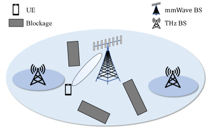
(a)

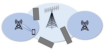
(b)

Figure 1: Illustration of DL and UL decoupled cell association in a 2-tier hybrid mmWave and THz network. (a) DL. (b) UL.

We adopt a flexible cell-association strategy where each UE connects to the BS that provides the strongest average biased received signal for both DL and UL communications. The average biased received power for the DL and UL at the typical UE from the nearest mmWave BS in the $\displaystyle m$-th tier is given by

$$P^{\mathrm{M},s}_{r,m}(R_{m})=P_{m}^{s}G_{m}^{\mathrm{max}}l^{\mathrm{M}}_{m}(R_{m})C_{m}^{s},$$ (10)

where $\displaystyle s\in\{\mathrm{DL,UL}\}$, $\displaystyle P_{m}^{\mathrm{DL}}$ is the DL transmit power of BSs in the $\displaystyle m$-th tier, $\displaystyle P_{m}^{\mathrm{UL}}$ is the UL transmit power of UE connected to the $\displaystyle m$-th tier, and $\displaystyle C_{m}^{\mathrm{DL}}$ and $\displaystyle C_{m}^{\mathrm{UL}}$ are the DL and UL cell-association bias factors of the $\displaystyle m$-th tier, respectively. If $\displaystyle C_{m}^{\mathrm{DL}}\left(C_{m}^{\mathrm{UL}}\right)>1$, more UEs will be offloaded to the $\displaystyle m$-th tier in the DL (UL) transmission. Similarly, the average biased received power for the DL and UL at the typical UE from the nearest THz BS in the $\displaystyle t$-th tier is given by

$$P^{\mathrm{T},s}_{r,t}(R_{t})=P_{t}^{s}G_{t}^{\mathrm{max}}l^{\mathrm{T}}_{t}(R_{t})C_{t}^{s},$$ (11)

where $\displaystyle s\in\{\mathrm{DL,UL}\}$.

III-A mmWave Cell Association

In the following Lemma, we derive the probability that the typical UE connects to an mmWave BS in the $\displaystyle m$-th tier.

Lemma 2.

The probability that the typical UE is associated with the $\displaystyle m$-th mmWave tier for the DL and UL is given by

$$\displaystyle\mathcal{A}^{s}_{m}=\int_{0}^{\infty}f_{R_{m}}(x)\times$$

$$\displaystyle\prod_{i\in\mathcal{M},i\neq m}\!\!\!\!\!\!\!\mathrm{exp}\!\left(\!\frac{2\pi\lambda_{i}e^{-(\zeta\Omega_{m,i}^{s}(x)+p)}\left(1\!-\!e^{\zeta\Omega_{m,i}^{s}(x)}\!+\!\zeta\Omega_{m,i}^{s}(x)\right)}{\zeta^{2}}\!\!\right)\times$$

$$\displaystyle\prod_{j\in\mathcal{T}}\!\!\mathrm{exp}\left(\!\frac{2\pi\lambda_{j}e^{-(\zeta\Psi_{m,j}^{s}(x)+p)}\!\!\left(\!1\!\!-\!e^{\zeta\Psi_{m,j}^{s}(x)}\!\!+\!\zeta\Psi_{m,j}^{s}(x)\!\right)}{\zeta^{2}}\!\!\right)\!\!\mathrm{d}x,$$ (12)

where $\displaystyle s\in\{\mathrm{DL,UL}\}$, $\displaystyle\Omega_{m,i}^{s}(x)=\left(\frac{C_{i}^{s}P_{i}^{s}N_{i}}{C_{m}^{s}P_{m}^{s}N_{m}}\right)^{\frac{1}{\alpha_{i}}}x^{\frac{\alpha_{m}}{\alpha_{i}}}$, and $\displaystyle\Psi_{m,j}^{s}(x)=\frac{\alpha_{j}}{K_{a}(f_{\mathrm{T}})}W_{\mathrm{L}}\left(\Lambda_{m,j}^{\mathrm{M},s}x^{\frac{\alpha_{m}}{\alpha_{j}}}\right)$, in which $\displaystyle W_{\mathrm{L}}(\cdot)$ is the Lambert W function with $\displaystyle x=W_{\mathrm{L}}(x)e^{W_{\mathrm{L}}(x)}$ and $\displaystyle\Lambda_{m,j}^{\mathrm{M},s}=\frac{K_{a}(f_{\mathrm{T}})}{\alpha_{j}}\left(\frac{f_{\mathrm{M}}^{2}P_{j}^{s}N_{j}C_{j}^{s}}{f_{\mathrm{T}}^{2}P_{m}^{s}N_{m}C_{m}^{s}}\right)^{\frac{1}{\alpha_{j}}}$.

Proof:

See Appendix A. ∎

Letting $\displaystyle X_{m}^{s}$, where $\displaystyle s\in\{\mathrm{DL,UL}\}$, be the distance from the serving BS to the typical UE, given that the typical UE is associated with a BS in the $\displaystyle m$-th mmWave tier, we characterise the PDF of $\displaystyle X_{m}^{s}$ in the following Lemma.

Lemma 3.

The PDF of the distance between the serving BS in the $\displaystyle m$-th mmWave tier and the typical UE for the DL and UL is given by

$$\displaystyle f_{X_{m}^{s}}(x)=\frac{f_{R_{m}}(x)}{\mathcal{A}^{s}_{m}}\times$$

$$\displaystyle\prod_{i\in\mathcal{M},i\neq m}\!\!\!\!\!\!\!\mathrm{exp}\!\!\left(\!\frac{2\pi\lambda_{i}e^{-(\zeta\Omega_{m,i}^{s}(x)+p)}\!\left(\!1\!-\!e^{\zeta\Omega_{m,i}^{s}(x)}\!+\!\zeta\Omega_{m,i}^{s}(x)\!\right)}{\zeta^{2}}\!\!\right)\!\!\times\!$$

$$\displaystyle\prod_{j\in\mathcal{T}}\!\mathrm{exp}\!\!\left(\!\frac{2\pi\lambda_{j}e^{-(\zeta\Psi_{m,j}^{s}(x)+p)}\!\left(\!1\!-\!e^{\zeta\Psi_{m,j}^{s}(x)}\!+\!\zeta\Psi_{m,j}^{s}(x)\!\right)}{\zeta^{2}}\!\!\right)\!\!.$$ (13)

Proof:

See Appendix B. ∎

III-B THz Cell Association

In the following Lemma, we present the probability that the typical UE connects to a THz BS in the $\displaystyle t$-th tier.

Lemma 4.

The probability that the typical UE is associated with the $\displaystyle t$-th THz tier for the DL and UL is given by

$$\displaystyle\mathcal{A}^{s}_{t}=\int_{0}^{\infty}f_{R_{t}}(x)\times$$

$$\displaystyle\prod_{i\in\mathcal{M}}\!\mathrm{exp}\!\!\left(\!\frac{2\pi\lambda_{i}e^{-(\zeta\Xi_{t,i}^{s}(x)+p)}\!\left(1-e^{\zeta\Xi_{t,i}^{s}(x)}+\zeta\Xi_{t,i}^{s}(x)\!\right)}{\zeta^{2}}\!\right)\!\times$$

$$\displaystyle\prod_{j\in\mathcal{T},j\neq t}\!\!\!\!\!\!\mathrm{exp}\!\!\left(\!\frac{2\pi\lambda_{j}e^{-(\zeta\Theta_{t,j}^{s}(x)+p)}\!\left(\!1\!-\!e^{\zeta\Theta_{t,j}^{s}(x)}\!+\!\zeta\Theta_{t,j}^{s}(x)\!\right)}{\zeta^{2}}\!\right)\!\mathrm{d}x,$$

where $\displaystyle s\!\in\!\{\mathrm{DL,UL}\}$, $\displaystyle\Xi_{t,i}^{s}(x)\!=\!\left(\frac{C_{i}^{s}P_{i}^{s}N_{i}f_{\mathrm{T}}^{2}}{C_{t}^{s}P_{t}^{s}N_{t}f_{\mathrm{M}}^{2}}\right)^{\frac{1}{\alpha_{i}}}e^{\frac{K_{a}(f_{\mathrm{T}})}{\alpha_{i}}x}x^{\frac{\alpha_{t}}{\alpha_{i}}}$ and $\displaystyle\Theta_{t,j}^{s}(x)=\frac{\alpha_{j}}{K_{a}(f_{\mathrm{T}})}W_{\mathrm{L}}(\Lambda_{t,j}^{\mathrm{T},s}e^{\frac{K_{a}(f_{\mathrm{T}})}{\alpha_{j}}x}x^{\frac{\alpha_{t}}{\alpha_{j}}})$, in which $\displaystyle\Lambda_{t,j}^{\mathrm{T},s}=\frac{K_{a}(f_{\mathrm{T}})}{\alpha_{j}}\left(\frac{C_{j}^{s}P_{j}^{s}N_{j}}{C_{t}^{s}P_{t}^{s}N_{t}}\right)^{\frac{1}{\alpha_{j}}}$.

Proof:

See Appendix C. ∎

Letting $\displaystyle X_{t}^{s}$, where $\displaystyle s\in\{\mathrm{DL,UL}\}$, be the distance from the serving BS to the typical UE, given that the typical UE is associated with a BS in the $\displaystyle t$-th THz tier, we characterise the PDF of $\displaystyle X_{t}^{s}$ in the Lemma below.

Lemma 5.

The PDF of the distance between the serving BS in the $\displaystyle t$-th THz tier and the typical UE for the DL and UL is given by

$$\displaystyle f_{X_{t}^{s}}(x)=\frac{f_{R_{t}}(x)}{\mathcal{A}^{s}_{t}}\times$$

$$\displaystyle\prod_{i\in\mathcal{M}}\!\mathrm{exp}\!\left(\!\frac{2\pi\lambda_{i}e^{-(\zeta\Xi_{t,i}^{s}(x)+p)}\!\left(1-e^{\zeta\Xi_{t,i}^{s}(x)}+\zeta\Xi_{t,i}^{s}(x)\!\right)}{\zeta^{2}}\!\right)\!\times$$

$$\displaystyle\prod_{j\in\mathcal{T},j\neq t}\!\!\!\!\!\mathrm{exp}\!\left(\!\frac{2\pi\lambda_{j}e^{-(\zeta\Theta_{t,j}^{s}(x)+p)}\!\left(1-e^{\zeta\Theta_{t,j}^{s}(x)}+\zeta\Theta_{t,j}^{s}(x)\!\right)}{\zeta^{2}}\!\right)\!.$$ (15)

Proof:

It follows similar proof as in Lemma 3. ∎

IV SINR and Rate Coverage in Hybrid mmWave and THz Networks

In this section, we will elaborate on the performance analysis in terms of SINR and rate coverage probabilities for the hybrid mmWave and THz networks based on the stochastic geometry framework.

IV-A SINR Coverage Probability

The SINR coverage probability is used to quantify the reliability of wireless transmissions and is the basis of quantifying other performance metrics. The DL (UL) SINR coverage probability is defined as the probability that the DL (UL) SINR of the typical UE is higher than a threshold $\displaystyle\tau$, which can be expressed as

$$\displaystyle P^{s}_{\mathrm{cov}}(\tau) \displaystyle=\sum_{m\in\mathcal{M}}\mathcal{A}^{s}_{m}P^{s}_{\mathrm{cov},m}(\tau)+\sum_{t\in\mathcal{T}}\mathcal{A}^{s}_{t}P^{s}_{\mathrm{cov},t}(\tau)$$

$$\displaystyle=\sum_{m\in\mathcal{M}}\mathcal{A}^{s}_{m}\int_{0}^{\infty}\mathbb{P}(\mathrm{SINR}^{s}_{m}(x)>\tau)f_{X_{m}^{s}}(x)\mathrm{d}x\,\,+$$

$$\displaystyle\quad\,\,\,\sum_{t\in\mathcal{T}}\mathcal{A}^{s}_{t}\int_{0}^{\infty}\mathbb{P}(\mathrm{SINR}^{s}_{t}(x)>\tau)f_{X_{t}^{s}}(x)\mathrm{d}x,$$ (16)

where $\displaystyle s\in\{\mathrm{DL,UL}\}$, $\displaystyle P_{\mathrm{cov},m}^{s}(\tau)$ and $\displaystyle P_{\mathrm{cov},t}^{s}(\tau)$ represent the SINR coverage probabilities of a typical UE when it is associated with the $\displaystyle m$-th mmWave tier and the $\displaystyle t$-th THz tier, respectively.

IV-A1 mmWave SINR Coverage Probability

When the typical UE is connected to the $\displaystyle m$-th mmWave tier, denoting $\displaystyle R_{m}=x$, the DL and UL received SINR can be expressed as

$$\displaystyle\mathrm{SINR}^{s}_{m}(x)=\frac{P_{m}^{s}G_{m}^{\mathrm{max}}l^{\mathrm{M}}_{m}(x)}{I_{m}^{\mathrm{M},s}+\delta_{m}^{2}},$$ (17)

where $\displaystyle s\!\in\!\{\mathrm{DL,UL}\}$, $\displaystyle\delta_{m}^{2}$ is the additive white Gaussian noise (AWGN) power, $\displaystyle I_{m}^{\mathrm{M},\mathrm{DL}}$ is the aggregated DL interference, which is given by

$$\displaystyle I_{m}^{\mathrm{M},\mathrm{DL}}=\sum\limits_{j\in\mathcal{M}}\sum\limits_{i\in\Phi_{j}^{\mathrm{L}}/B_{\mathrm{S},m}^{\mathrm{DL}}}P^{\mathrm{DL}}_{j}G_{j}(N_{j},\phi_{{D}_{i,j}})l^{\mathrm{M}}_{j}(d_{i,j}),$$ (18)

where $\displaystyle B_{\mathrm{S},m}^{\mathrm{DL}}$ is the DL serving BS, $\displaystyle\Phi^{\mathrm{L}}_{j}$ is the set of LOS BSs in the $\displaystyle j$-th tier, and $\displaystyle d_{i,j}$ is the distance from BS $\displaystyle i$ in the $\displaystyle j$-th tier to the typical UE, and $\displaystyle I_{m}^{\mathrm{M},\mathrm{UL}}$ is the aggregated UL interference, which is given by

$$\displaystyle I_{m}^{\mathrm{M},\mathrm{UL}}=\sum\limits_{j\in\mathcal{M}}\sum\limits_{u\in\Phi_{\mathrm{U},j}^{\mathrm{L}}/U_{0}}P^{\mathrm{UL}}_{j}G_{j}(N_{j},\phi_{{D}_{u,j}^{\mathrm{UL}}})l^{\mathrm{M}}_{j}(d_{u,j}^{\mathrm{UL}}),$$ (19)

where $\displaystyle U_{0}$ is the typical UE, $\displaystyle\Phi_{\mathrm{U},j}^{\mathrm{L}}$ is the set of LOS UE connected to the $\displaystyle j$-th tier, $\displaystyle\phi_{{D}_{u,j}^{\mathrm{UL}}}=\frac{1}{2}\left(\mathrm{cos}\phi_{U_{u,j}}-\mathrm{cos}\phi_{S_{u,j}^{\mathrm{UL}}}\right)$, in which $\displaystyle U_{u,j}$ denotes UE $\displaystyle u$ in the $\displaystyle j$-th tier, $\displaystyle\phi_{U_{u,j}}$ is the azimuth angle between $\displaystyle U_{u,j}$ and the typical BS that serves the typical UE, and $\displaystyle\phi_{S_{u,j}^{\mathrm{UL}}}$ is the azimuth angle between $\displaystyle U_{u,j}$ and its serving BS, and $\displaystyle d_{u,j}^{\mathrm{UL}}$ is the distance from $\displaystyle U_{u,j}$ to the typical BS. Due to orthogonal time/frequency resource partitioning, on each resource block, the locations of interfering UE can be approximated as those of interfering BSs as follows [19, 26]

$$\displaystyle I_{m}^{\mathrm{M},\mathrm{UL}}\approx\sum\limits_{j\in\mathcal{M}}\sum\limits_{i\in\Phi_{j}^{\mathrm{L}}/B_{\mathrm{S},m}^{\mathrm{UL}}}P^{\mathrm{UL}}_{j}G_{j}(N_{j},\phi_{{D}_{i,j}})l^{\mathrm{M}}_{j}(d_{i,j}),$$ (20)

where $\displaystyle B_{\mathrm{S},m}^{\mathrm{UL}}$ is the UL serving BS.

According to the predefined SINR in (17), we derive the conditional coverage probability when the typical UE connects to an mmWave tier.

Theorem 1.

The conditional coverage probability for the DL and UL when the typical UE is connected to the $\displaystyle m$-th tier mmWave network is given by

$$\displaystyle\mathbb{P}(\mathrm{SINR}^{s}_{m}>\tau)$$

$$\displaystyle\approx\sum_{n=1}^{\gamma_{m}}(-1)^{n+1}\left(\begin{subarray}{c}\gamma_{m}\\ \\ n\end{subarray}\right)\mathrm{exp}\left(-V_{m}^{s}O_{m}\right)\times$$

$$\displaystyle\prod\limits_{j\in\!\mathcal{M}}\prod\limits_{w\in\!\{\mathrm{max},\mathrm{min}\}}\!\!\!\!\!\!\!\!\!\mathrm{exp}\!\!\left(\!-\!2\pi\lambda_{j}P_{\mathrm{G},j}^{w}\!\!\int_{Z_{m,j}^{s}}^{\infty}\!\!\!\!\!\!\left[1\!-\!\Delta_{m,j}^{s,w}(r)\right]P_{\mathrm{LOS}}(r)r\mathrm{d}r\!\right)\!,$$ (21)

where $\displaystyle s\in\{\mathrm{DL,UL}\}$, $\displaystyle P_{\mathrm{G},j}^{\mathrm{max}}=\phi_{\mathrm{3dB},j}/0.5=2\phi_{\mathrm{3dB},j}$ is the probability that the typical UE (BS) is located in the main-lobe direction, $\displaystyle P_{\mathrm{G},j}^{\mathrm{min}}=1-P_{\mathrm{G},j}^{\mathrm{max}}$ is the probability that the typical UE (BS) is located in the side-lobe direction, $\displaystyle O_{m}=\delta_{m}^{2}\left(\frac{4\pi f_{\mathrm{M}}}{c}\right)^{2}$, $\displaystyle V_{m}^{s}=\frac{n\eta_{m}\tau x^{\alpha_{m}}}{P_{m}^{s}N_{m}}$, $\displaystyle\eta_{m}=\gamma_{m}(\gamma_{m}!)^{-\frac{1}{\gamma_{m}}}$, $\displaystyle\Delta_{m,j}^{s,w}(r)=\left(1+\frac{V_{m}^{s}P_{j}^{s}G_{j}^{w}r^{-\alpha_{j}}}{\gamma_{m}}\right)^{-\gamma_{m}}$, and $\displaystyle Z_{m,j}^{s}=\left(\frac{C_{j}^{s}P_{j}^{s}N_{j}}{C_{m}^{s}P_{m}^{s}N_{m}}\right)^{\frac{1}{\alpha_{j}}}x^{\frac{\alpha_{m}}{\alpha_{j}}}$.

Proof:

See Appendix D. ∎

IV-A2 THz SINR Coverage Probability

When the typical UE is connected to the $\displaystyle t$-th THz tier, denoting $\displaystyle R_{t}=x$, the DL and UL received SINR can be expressed as

$$\displaystyle\mathrm{SINR}^{s}_{t}(x) \displaystyle=\frac{P_{t}^{s}G_{t}^{\mathrm{max}}l^{\mathrm{T}}_{t}(x)}{I_{t}^{\mathrm{T},s}+\mathrm{Noise}_{t}^{s}(x)},$$ (22)

where $\displaystyle s\in\{\mathrm{DL,UL}\}$, $\displaystyle I_{t}^{\mathrm{T},s}$ is the aggregated interference, and $\displaystyle\mathrm{Noise}_{t}^{s}$ is the cumulative molecular absorption and thermal noises. More specifically, the DL aggregated interference is given by

$$\displaystyle I_{t}^{\mathrm{T},\mathrm{DL}}$$

$$\displaystyle=\sum\limits_{j\in\mathcal{T}}\sum\limits_{i\in\Phi_{j}^{\mathrm{L}}/B_{\mathrm{S},t}^{\mathrm{DL}}}P^{\mathrm{DL}}_{j}G_{j}(N_{j},\phi_{{D}_{i,j}})l^{\mathrm{M}}_{j}(d_{i,j})$$

$$\displaystyle=\!\!\sum\limits_{j\in\mathcal{T}}\sum\limits_{i\in\Phi_{j}^{\mathrm{L}}/B_{\mathrm{S},t}^{\mathrm{DL}}}\!\!P^{\mathrm{DL}}_{j}G_{j}(N_{j},\phi_{{D}_{i,j}})\!\!\left(\frac{c}{4\pi f_{\mathrm{T}}}\right)^{\!2\!}\!\!d_{i,j}^{-\alpha_{t}}e^{-\!K_{a}(f_{\mathrm{T}})d_{i,j}},$$ (23)

where $\displaystyle B_{\mathrm{S},t}^{\mathrm{DL}}$ is the DL serving BS. The DL total noise power is given by

$$\displaystyle\mathrm{Noise}_{t}^{\mathrm{DL}}(x)$$

$$\displaystyle=\!\!\sum\limits_{j\in\mathcal{T}}\sum\limits_{i\in\Phi_{j}^{\mathrm{L}}\!/\!B_{\mathrm{S},t}^{\mathrm{DL}}}\!\!\!\!\!\!\!P^{\mathrm{DL}}_{j}G_{j}\!\!\left(\!N_{j},\phi_{{D}_{i,j}}\!\right)\!\!\left(\!\!\frac{c}{4\pi f_{\mathrm{T}}}\!\!\right)^{\!\!2\!}\!d_{i,j}^{-\alpha_{t}}\!\!\left(\!1\!-\!e^{-\!K_{a}(f_{\mathrm{T}})d_{i,j}}\!\right)$$

$$\displaystyle\ +P_{t}^{\mathrm{DL}}G_{t}^{\mathrm{max}}\left(\frac{c}{4\pi f_{\mathrm{T}}}\right)^{2}x^{-\alpha_{t}}\left(1-e^{-K_{a}(f_{\mathrm{T}})x}\right)+\delta_{t}^{2},$$ (24)

where the first two terms represent the molecular absorption noise from the interference signals and the desired signal, respectively, and $\displaystyle\delta_{t}^{2}$ is the Johnson-Nyquist noise generated by thermal agitation of electrons in conductors [27], which is given by $\displaystyle\delta_{t}^{2}=\left(\frac{B_{\mathrm{W},t}\lambda^{2}}{4\pi}\right)k_{\mathrm{B}}T_{0}$, where $\displaystyle B_{\mathrm{W},t}$ is the bandwidth of the $\displaystyle t$-th THz tier, $\displaystyle\lambda$ is the wavelength, $\displaystyle k_{\mathrm{B}}$ is the Boltzmann constant, and $\displaystyle T_{0}$ is the temperature in Kelvin. Combining (IV-A2) and (IV-A2), we have

$$\displaystyle I_{t}^{\mathrm{T},\mathrm{DL}}+\mathrm{Noise}_{t}^{\mathrm{DL}}(x)$$

$$\displaystyle=\sum\limits_{j\in\mathcal{T}}\sum\limits_{i\in\Phi_{j}^{\mathrm{L}}/B_{\mathrm{S},t}^{\mathrm{DL}}}P^{\mathrm{DL}}_{j}G_{j}\left(N_{j},\phi_{{D}_{i,j}}\right)\left(\frac{c}{4\pi f_{\mathrm{T}}}\right)^{2}d_{i,j}^{-\alpha_{t}}+$$

$$\displaystyle\quad\ P_{t}^{\mathrm{DL}}G_{t}^{\mathrm{max}}\left(\frac{c}{4\pi f_{\mathrm{T}}}\right)^{2}x^{-\alpha_{t}}\left(1-e^{-K_{a}(f_{\mathrm{T}})x}\right)+\delta_{t}^{2}.$$ (25)

Following the approximation in (20), we have the following expression for the UL transmission

$$\displaystyle I_{t}^{\mathrm{T},\mathrm{UL}}+\mathrm{Noise}_{t}^{\mathrm{UL}}(x)$$

$$\displaystyle\approx\sum\limits_{j\in\mathcal{T}}\sum\limits_{i\in\Phi_{j}^{\mathrm{L}}/B_{\mathrm{S},t}^{\mathrm{UL}}}P_{j}^{\mathrm{UL}}G_{j}\left(N_{j},\phi_{{D}_{i,j}}\right)\left(\frac{c}{4\pi f_{\mathrm{T}}}\right)^{2}d_{i,j}^{-\alpha_{t}}+$$

$$\displaystyle\quad P_{t}^{\mathrm{UL}}G_{t}^{\mathrm{max}}\left(\frac{c}{4\pi f_{\mathrm{T}}}\right)^{2}x^{-\alpha_{t}}\left(1-e^{-K_{a}(f_{\mathrm{T}})x}\right)+\delta_{t}^{2}.$$ (26)

When the typical UE is connecting to the $\displaystyle t$-th tier THz network, the conditional coverage probability can be derived based on the SINR in (22).

Theorem 2.

The conditional coverage probability for the DL and UL when the typical UE is connected to the $\displaystyle t$-th tier THz network is given by

$$\displaystyle\mathbb{P}(\mathrm{SINR}^{s}_{t}(x)>\tau)$$

$$\displaystyle\approx\!\!\sum_{n=1}^{\gamma_{\mathrm{T}}}\!(-1)^{n+1}\!\!\left(\begin{subarray}{c}\gamma_{\mathrm{T}}\\ \\ n\end{subarray}\right)\!\mathrm{exp}\!\Bigg{[}\!\!-\!n\eta_{\mathrm{T}}\tau\bigg{(}\!\frac{\delta_{t}^{2}e^{K_{a}(f_{\mathrm{T}})x}}{J_{t}^{s}(x)}+e^{K_{a}(f_{\mathrm{T}})x}\!-\!\!1\!\!\bigg{)}\!\Bigg{]}\!$$

$$\displaystyle\quad\ \ \ \ \times\prod\limits_{j\in\mathcal{T}}\prod\limits_{w\in\{\mathrm{max},\mathrm{min}\}}\mathrm{exp}\Bigg{[}-2\pi\lambda_{j}P_{\mathrm{G},j}^{w}\int_{Z_{t,j}^{s}}^{\infty}P_{\mathrm{LOS}}(r)r$$

$$\displaystyle\qquad\ \times\Bigg{(}1-\mathrm{exp}\bigg{(}-n\eta_{\mathrm{T}}\tau x^{\alpha_{t}}e^{K_{a}(f_{\mathrm{T}})x}\frac{P_{j}^{s}G_{j}^{w}}{P_{t}^{s}N_{t}}r^{-\alpha_{t}}\bigg{)}\Bigg{)}\mathrm{d}r\Bigg{]},$$ (27)

where $\displaystyle\gamma_{\mathrm{T}}$ is the shape parameter of the induced Nakagami-$\displaystyle m$ distribution $\displaystyle h_{\mathrm{T}}\sim\Gamma(\gamma_{\mathrm{T}},\frac{1}{\gamma_{\mathrm{T}}})$ (when $\displaystyle\gamma_{\mathrm{T}}\rightarrow\infty$, $\displaystyle h_{\mathrm{T}}\rightarrow 1$), $\displaystyle\eta_{\mathrm{T}}=\gamma_{\mathrm{T}}(\gamma_{\mathrm{T}}!)^{-\frac{1}{\gamma_{\mathrm{T}}}}$, $\displaystyle J_{t}^{s}(x)=P_{t}^{s}G_{t}^{\mathrm{max}}\left(\frac{c}{4\pi f_{\mathrm{T}}}\right)^{2}x^{-\alpha_{t}}$, and $\displaystyle Z_{t,j}^{s}=\frac{\alpha_{j}}{K_{a}(f_{\mathrm{T}})}W_{\mathrm{L}}(\Lambda_{t,j}^{\mathrm{T},s}e^{\frac{K_{a}(f_{\mathrm{T}})}{\alpha_{j}}x}x^{\frac{\alpha_{t}}{\alpha_{j}}})$, where the $\displaystyle\Lambda_{t,j}^{\mathrm{T},s}$ is defined in Lemma 4.

Proof:

It follows similar proof as in Theorem 1. ∎

IV-B Rate Coverage Probability

Due to the abundant bandwidths, mmWave/THz frequency bands can provide ultra-high data rate. In this respect, rate coverage probability is a crucial performance metric that assesses the capacity of a wireless network to ensure reliable communication at a specific data rate over a certain geographic region. The DL (UL) rate coverage probability is defined as the probability that the DL (UL) rate is higher than a given threshold as follows

$$\displaystyle R_{\mathrm{cov}}^{s}(\rho) \displaystyle=\sum_{k=1}^{K}R_{\mathrm{cov},k}^{s}(\rho)\mathcal{A}_{k}^{s},$$ (28)

where $\displaystyle s\in\{\mathrm{DL,UL}\}$, $\displaystyle\rho$ is the rate threshold, and $\displaystyle R_{\mathrm{cov},k}^{s}(\rho)$ is the conditional rate coverage probability when the typical UE is associated with the $\displaystyle k$-th tier. The conditional rate coverage probability can be further derived as

$$\displaystyle R_{\mathrm{cov},k}^{s}(\rho) \displaystyle=\mathbb{E}_{x}\left[\mathbb{P}(\frac{B_{\mathrm{W},k}}{S_{k}^{s}}\mathrm{log}_{2}(1+\mathrm{SINR}_{k}^{s}(x))>\rho)\right]$$

$$\displaystyle=\mathbb{E}_{x}\left[\mathbb{P}(\mathrm{SINR}_{k}^{s}(x)>2^{\frac{\rho S_{k}^{s}}{B_{\mathrm{W},k}}}-1)\right],$$ (29)

where $\displaystyle B_{\mathrm{W},k}$ is the bandwidth of the $\displaystyle k$-th tier and $\displaystyle S_{k}^{s}$ is the average number of UEs served by a BS in the $\displaystyle k$-th tier, which is given by [28]

$$\displaystyle S_{k}^{s}=1+\frac{1.28\lambda_{\mathrm{U}}\mathcal{A}_{k}^{s}}{\lambda_{k}}.$$ (30)

According to (28) and (IV-B), the rate coverage probability for the DL and UL can be derived as

$$\displaystyle R^{s}_{\mathrm{cov}}(\rho)$$

$$\displaystyle=\sum_{m\in\mathcal{M}}R^{s}_{\mathrm{cov},m}(\rho)\mathcal{A}^{s}_{m}+\sum_{t\in\mathcal{T}}R^{s}_{\mathrm{cov},t}(\rho)\mathcal{A}^{s}_{t}$$

$$\displaystyle=\!\!\sum_{m\in\mathcal{M}}P_{\mathrm{cov},m}^{s}\!\left(2^{\frac{\rho S_{m}^{s}}{B_{\mathrm{W},m}}}\!\!-\!\!1\right)\mathcal{A}^{s}_{m}\!+\!\sum_{t\in\mathcal{T}}P_{\mathrm{cov},t}^{s}\!\left(2^{\frac{\rho S_{t}^{s}}{B_{\mathrm{W},t}}}\!\!-\!\!1\right)\mathcal{A}^{s}_{t}.$$ (31)

V Numerical Results

In this section, we validate the derived analytical expressions with Monte Carlo simulations. Each simulation consists of $\displaystyle 5\times 10^{4}$ independent random realisations according to the system model described in Section II. The default numerical simulation parameter values are listed in Table II unless otherwise stated [29, 7, 17, 30], where subscript 1 denotes the mmWave tier and subscript 2 denotes the THz tier. The impacts of different system parameters on the association probability, SINR coverage probability and rate coverage probability are investigated.

TABLE II: Value of Parameters

Parameters	Default value
$\displaystyle\lambda_{\mathrm{b}}$, $\displaystyle\lambda_{\mathrm{U}}$	$\displaystyle 10^{-3}$ $\displaystyle\mathrm{m}^{-2}$, $\displaystyle 2\times 10^{-3}$ $\displaystyle\mathrm{m}^{-2}$
$\displaystyle L$, $\displaystyle W$	15 m, 15 m
$\displaystyle\lambda_{1}$, $\displaystyle\lambda_{2}$	$\displaystyle 5\times 10^{-5}$ $\displaystyle\mathrm{m}^{-2}$, $\displaystyle 5\times 10^{-4}$ $\displaystyle\mathrm{m}^{-2}$
$\displaystyle N_{1}$, $\displaystyle N_{2}$	32, 64
$\displaystyle\alpha_{1}$, $\displaystyle\alpha_{2}$	2, 2
$\displaystyle\gamma_{1}$, $\displaystyle\gamma_{\mathrm{T}}$	3, 10
$\displaystyle P_{1}^{\mathrm{DL}}$, $\displaystyle P_{2}^{\mathrm{DL}}$	33 dBm, 23 dBm
$\displaystyle P_{1}^{\mathrm{UL}}$, $\displaystyle P_{2}^{\mathrm{UL}}$	23 dBm, 23 dBm
$\displaystyle f_{\mathrm{M}}$, $\displaystyle f_{\mathrm{T}}$	28 GHz, 340 GHz
$\displaystyle C_{1}^{s}$, $\displaystyle C_{2}^{s},s\in\{\mathrm{DL,UL}\}$	1, 1
$\displaystyle K_{a}(f_{\mathrm{T}})$	0.01
$\displaystyle\delta_{1}^{2}$	$\displaystyle-174\,\mathrm{dBm/Hz}+10\mathrm{log}_{10}(B_{\mathrm{W},1})+10\,\mathrm{dB}$
$\displaystyle B_{\mathrm{W},1}$, $\displaystyle B_{\mathrm{W},2}$	1 GHz, 10 GHz
$\displaystyle k_{\mathrm{B}}$	$\displaystyle 1.3806\times 10^{-23}\mathrm{J}/\mathrm{K}$
$\displaystyle T_{0}$	300.15 K
$\displaystyle\tau$, $\displaystyle\rho$	10 dB, $\displaystyle 10^{9}$ bit/s

V-A Association Probability

Fig. 2 presents the DL and UL association probabilities versus the ratio of THz to mmWave BS density. It is clear that the analytical results align well with the simulation results, validating the correctness of our derived theoretical expressions. The THz tier benefits from the increase of THz BSs for both DL and UL transmissions. On the other hand, a notable difference between DL and UL association probabilities is observed, indicating that the typical UE is inclined to connect to different BSs during DL and UL associations. This disparity increases with the density ratio of THz BSs to mmWave BSs. It is noteworthy that when there are only mmWave BSs, i.e., $\displaystyle\lambda_{2}=0$ $\displaystyle\mathrm{m}^{-2}$, the sum of probabilities connecting to the mmWave tier and the THz tier is only about 0.5. This indicates that in a network with a low BS density, a UE may not be able to connect to a BS due to the presence of blockages. This concern is eliminated when $\displaystyle\lambda_{2}$ increases to around $\displaystyle 5\lambda_{1}$, demonstrating the necessity of deploying dense networks in high-frequency communications.

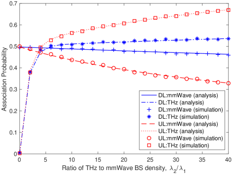
Figure 2: The analytical and simulation results of the association probability versus the ratio of THz to mmWave BS density ($\displaystyle\lambda_{2}/\lambda_{1}$).

In Fig. 3, the DL and UL association probabilities are plotted versus the bias factor of the THz tier. It is observed that the association probability of the THz tier monotonically increases with the bias factor. This result is quite intuitive because more UE are encouraged to connect with the THz BSs when the bias factor of the THz tier increases. Another observation is that the probability of connecting to the mmWave tier in the DL is always higher than that in the UL, as the DL transmit power of mmWave BSs is higher than that of THz BSs.

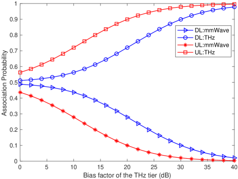
Figure 3: The analytical results of the association probability versus the bias factor of the THz tier.

V-B SINR and Rate Coverage Probabilities

Fig. 4 shows the DL and UL SINR coverage probabilities versus the SINR threshold, where we present results for 2-tier and 3-tier hybrid mmWave/THz networks. The 1st mmWave tier in the 3-tier hybrid network has the following simulation parameters: $\displaystyle\lambda_{1}=10^{-5}\ \mathrm{m}^{-2}$, $\displaystyle N_{1}=16$, $\displaystyle P_{1}^{\mathrm{DL}}=43$ dBm, and $\displaystyle P_{1}^{\mathrm{UL}}=23$ dBm. The 2nd mmWave tier and the THz tier have the same simulation parameters as the default values listed in Table II. The figure demonstrates that the analytical expressions provide accurate results that closely match the simulation curves, which allows us to use the analytical expressions for the following results. Thanks to the extra deployment of an mmWave tier, the 3-tier hybrid network has a higher SINR coverage probability than the 2-tier network. For clear exposition, we use the 2-tier hybrid network in the following analysis.

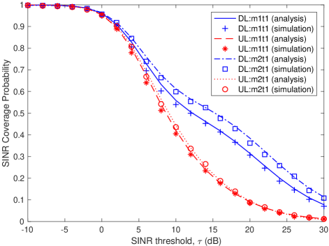
Figure 4: The analytical and simulation results of the SINR coverage probability versus the SINR threshold ($\displaystyle\tau$). We present results of a 2-tier hybrid network (m1t1) consisting of 1 tier of mmWave network and 1 tier of THz network, and a 3-tier hybrid network (m2t1) consisting of 2 tiers of mmWave networks and 1 tier of THz network.

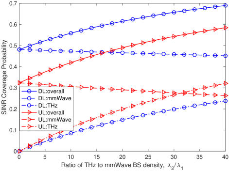
Figure 5: The analytical results of the SINR coverage probability versus the ratio of THz to mmWave BS density ($\displaystyle\lambda_{2}/\lambda_{1}$).

In Fig. 5, the DL and UL SINR coverage probabilities are presented versus the ratio of THz to mmWave BS density. We can see that the overall SINR coverage probability increases with the THz BS density due to the increased probability of connecting to an LOS BS and the reduced THz propagation loss. Due to the higher transmission power, the contribution of mmWave tier to the SINR coverage probability in the DL transmission is higher than that in the UL transmission.

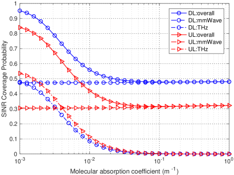
Figure 6: The analytical results of the SINR coverage probability versus the molecular absorption coefficient $\displaystyle K_{a}\left(f_{\mathrm{T}}\right)$.

In Fig. 6, the DL and UL SINR coverage probabilities are depicted versus the molecular absorption coefficient of the THz tier. Note that our theoretical expressions are valid for any molecular absorption coefficient value $\displaystyle K_{a}(f_{\mathrm{T}})$, which depends on the transmission environment and signal frequency. As can be observed, a higher molecular absorption coefficient generally leads to the decay of the SINR coverage probability. When $\displaystyle K_{a}(f_{\mathrm{T}})>0.1\mathrm{m}^{-1}$, the SINR coverage probability of the THz tier approaches zero as all UEs preferentially connect to the mmWave tier. This results in a slight increase in the overall SINR coverage probability due to more favourable propagation conditions in the mmWave layer.

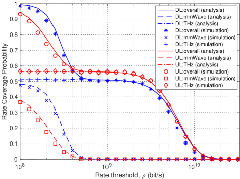
Figure 7: The analytical and simulation results of the rate coverage probability versus the rate threshold $\displaystyle\rho$.

Fig. 7 presents the DL and UL rate coverage probabilities against the rate threshold. The figure highlights that the analytical results yield accurate results, which align closely with the simulation results. As demonstrated in the figure, due to the limited bandwidth, the mmWave tier fails to contribute any rate coverage probability when the rate threshold is above $\displaystyle 10^{8.5}$ bit/s, indicating that only the THz tier is capable of providing a rate higher than $\displaystyle 10^{8.5}$ bit/s. In Fig. 8, we increase the THz BS density to $\displaystyle\lambda_{t}=8\times 10^{-4}$ bit/s to evaluate the DL and UL rate coverage probabilities. Compared with Fig. 7, the rate coverage probability has a significant increase. This is because each BS serves a smaller number of UEs when more BSs are deployed, and thus each UE can benefit from a larger bandwidth.

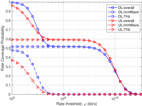
Figure 8: The analytical results of the rate coverage probability versus the rate threshold with THz BS density $\displaystyle\lambda_{2}=8\times 10^{-4}$ $\displaystyle\mathrm{m}^{-2}$.

V-C Effect of DL and UL Decoupled Cell Association

In this part we show the effect of the bias factor on the SINR and rate coverage, and illustrate the necessity of using DL and UL decoupled cell-association strategy.

In Fig. 9, we show the DL and UL SINR coverage probabilities versus the bias factor of the THz tier, where $\displaystyle P_{k}^{\mathrm{UL}}$ denotes the UL transmit power in the $\displaystyle k$-th tier and $\displaystyle P_{k}^{\mathrm{UL}}=P_{k^{{}^{\prime}}}^{\mathrm{UL}},\forall k^{{}^{\prime}}\in\mathcal{K}$ and $\displaystyle k^{{}^{\prime}}\neq k$. In the DL and UL coupled cell-association strategy, the typical UE connects to the BS providing the strongest DL average biased received power for both DL and UL communications. It is observed that the SINR coverage probability first increases and then decreases with the bias factor of the THz tier for all the cases considered. The initial increase comes from the increase of the contribution of the THz tier when the probability of connecting to the THz tier increases. On the other hand, the THz tier suffers from a high penetration loss, as a result of which, a further increased bias factor lead to the decay of the SINR coverage. DL and UL transmissions may have different optimal bias factors that maximise the SINR coverage. From Fig. 9(a), the optimal bias for the DL case is $\displaystyle-0.5$ dB, while the optimal values for the two coupled UL cases are 10.4 dB and 18.6 dB, respectively. As such, the DL and UL coupled cell association cannot ensure maximum SINR coverage for both DL and UL transmissions simultaneously. In contrast, this can be achieved by the DL and UL decoupled cell-association strategy due to separately designed bias factors. Interestingly, from Fig. 9(b), we can see that for a small THz BS density, the SINR coverage probability only experiences a slight increase at the beginning of increasing the bias factor. Specially, consider the case where the priority of the DL transmission is to achieve the maximum rate and set the bias factor to 26 dB; the SINR coverage probabilities of the DL case and coupled UL case ($\displaystyle P_{k}^{\mathrm{UL}}=23$ dBm) are 0.39 and 0.29, respectively. However, the priority of the UL transmission may not be the maximum rate but the most reliable transmission, in which case a smaller bias factor is more preferable. In summary, it is difficult for the DL and UL coupled cell-association strategy to ensure good performance for both DL and UL transmissions.

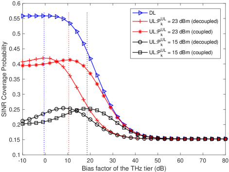
(a)

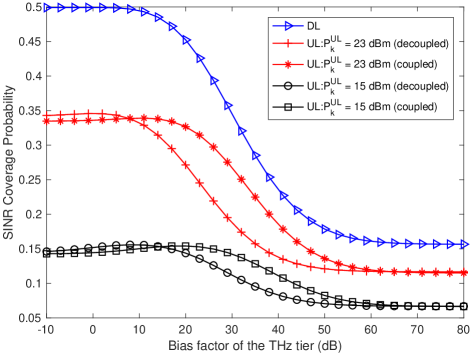
(b)

Figure 9: The analytical results of the SINR coverage probability versus the bias factor of the THz tier. (a) $\displaystyle\lambda_{2}=5\times 10^{-4}\ \mathrm{m}^{-2}$. (b) $\displaystyle\lambda_{2}=10^{-4}\ \mathrm{m}^{-2}$.

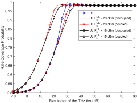
(a)

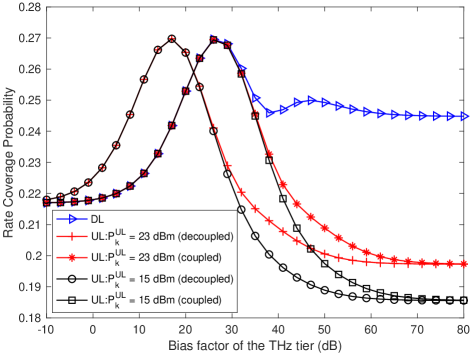
(b)

Figure 10: The analytical results of the rate coverage probability versus the bias factor of the THz tier. (a) $\displaystyle\lambda_{2}=5\times 10^{-4}\ \mathrm{m}^{-2}$. (b) $\displaystyle\lambda_{2}=10^{-4}\ \mathrm{m}^{-2}$.

In Fig. 10, we plot the rate coverage probability versus the bias factor of the THz tier. From Fig. 10(a), it is observed that the rate coverage probability first increases and then slightly decreases with the bias factor. The UE benefits from a larger bandwidth when the bias factor increases. Nevertheless, when the bias factor exceeds a critical threshold, the rate coverage suffers from a low SINR and excessive UE per THz BS. If the rate coverage objective is set to 0.9, we can see that a bias factor of 26 dB is enough for the DL case, but yields rate coverage probabilities of 0.85 and 0.83 for the two coupled UL cases, respectively, indicating the necessity of using DL and UL decoupled cell association. From Fig. 10(b), we can observe that the rate coverage decreases rapidly with the bias factor after reaching a peak value. This is a result of the insufficient bandwidth per UE under a small THz BS density.

From Fig. 9 and Fig. 10, we can summarise two important system design insights. First, there exists a trade-off between SINR and rate when choosing the bias factor. The optimal bias factor that maximises the rate coverage generally results in a low SINR coverage, which leads to the need for robust modulation and coding techniques. Second, the advantage of the DL and UL decoupled cell-association strategy over its coupled counterpart is more significant as the density of THz BSs increases. Given the dense deployment of THz BSs in the future, this highlights the importance of applying the DL and UL decoupled cell-association strategy.

VI Conclusions

In this paper, we have proposed a novel and tractable stochastic geometry-based framework for the performance evaluation of a general multi-tier hybrid mmWave and THz network. We have investigated the DL and UL decoupled cell-association strategy that allows the separate cell access during the DL and UL transmissions. Under the DL and UL decoupled cell-association strategy, we have derived novel SINR and rate coverage probability expressions for DL and UL transmissions, respectively, incorporating the LOS probability model, beamforming gain per BS, cell-association bias and molecular absorption effect of the THz band. Our numerical results reveal that a significant increase in both SINR and rate coverage probabilities of the hybrid mmWave and THz network can be achieved by raising the THz BS density. It is noteworthy that the propagation loss and noise caused by molecular absorption in the THz band have an adverse impact on the SINR coverage probability. Moreover, we have demonstrated that the DL and UL decoupled cell-association strategy enables a more flexible bias factor design that ensures good SINR and rate coverage for both DL and UL communications. In the future, we will extend the proposed framework to study the effects of beam misalignment and UE mobility. The performance evaluation of wireless extended reality in hybrid mmWave and THz networks is also of future interest.

Appendix A Proof of Lemma 2

Under the strongest average biased received signal cell-association strategy, the typical UE connects to the $\displaystyle m$-th mmWave tier for the DL and UL if $\displaystyle P^{\mathrm{M},s}_{r,m}(R_{m})>\mathop{\mathrm{max}}\limits_{i\in\mathcal{M},i\neq m}P^{\mathrm{M},s}_{r,i}(R_{i})$ and $\displaystyle P^{\mathrm{M},s}_{r,m}(R_{m})>\mathop{\mathrm{max}}\limits_{j\in\mathcal{T}}P^{\mathrm{T},s}_{r,j}(R_{j})$, where $\displaystyle s\in\{\mathrm{DL,UP}\}$. Denoting $\displaystyle R_{m}=x$, the association probability of a typical UE served by the nearest mmWave BS in the $\displaystyle m$-th tier can be derived as

$$\displaystyle\mathcal{A}^{s}_{m}=\mathbb{E}_{x}\Bigg{[} \displaystyle\mathbb{P}\left[P^{\mathrm{M},s}_{r,m}(x)>\mathop{\mathrm{max}}\limits_{i\in\mathcal{M},i\neq m}P^{\mathrm{M},s}_{r,i}(R_{i})\right]\times$$

$$\displaystyle\ \ \ \ \ \ \ \ \ \ \ \mathbb{P}\left[P^{\mathrm{M},s}_{r,m}(x)>\mathop{\mathrm{max}}\limits_{j\in\mathcal{T}}P^{\mathrm{T},s}_{r,j}(R_{j})\right]\Bigg{]},$$ (32)

where $\displaystyle s\in\{\mathrm{DL,UL}\}$. Substituting (10) and (11) into (A), we have

$$\displaystyle\mathbb{P}\left[P^{\mathrm{M},s}_{r,m}(x)>\mathop{\mathrm{max}}\limits_{i\in\mathcal{M},i\neq m}P^{\mathrm{M},s}_{r,i}(R_{i})\right]$$

$$\displaystyle=\prod_{i\in\mathcal{M},i\neq m}\mathbb{P}\left[P_{m}^{s}G_{m}^{\mathrm{max}}l^{\mathrm{M}}_{m}(x)C_{m}^{s}>P_{i}^{s}G_{i}^{\mathrm{max}}l^{\mathrm{M}}_{i}(R_{i})C_{i}^{s}\right]$$

$$\displaystyle=\prod_{i\in\mathcal{M},i\neq m}\mathbb{P}\Bigg{[}P_{m}^{s}N_{m}\left(\frac{c}{4\pi f_{\mathrm{M}}}\right)^{2}x^{-\alpha_{m}}C_{m}^{s}>$$

$$\displaystyle\ \ \ \ \ \ \ \ \ \ \ \ \ \ \ \ \ \qquad\quad\qquad P_{i}^{s}N_{i}\left(\frac{c}{4\pi f_{\mathrm{M}}}\right)^{2}R_{i}^{-\alpha_{i}}C_{i}^{s}\Bigg{]}$$

$$\displaystyle=\prod_{i\in\mathcal{M},i\neq m}\mathbb{P}\left[R_{i}>\left(\frac{C_{i}^{s}P_{i}^{s}N_{i}}{C_{m}^{s}P_{m}^{s}N_{m}}\right)^{\frac{1}{\alpha_{i}}}x^{\frac{\alpha_{m}}{\alpha_{i}}}\right]$$

$$\displaystyle\overset{(a)}{=}\prod_{i\in\mathcal{M},i\neq m}\mathrm{exp}\left(-2\pi\lambda_{i}\int_{0}^{\Omega_{m,i}^{s}(x)}P_{\mathrm{LOS}}(u)u\mathrm{d}u\right)$$

$$\displaystyle=\prod_{i\in\mathcal{M},i\neq m}\mathrm{exp}\Bigg{(}-2\pi\lambda_{i}e^{-(\zeta\Omega_{m,i}^{s}(x)+p)}\quad\times$$

$$\displaystyle\ \ \ \ \ \ \ \qquad\qquad\qquad\quad\quad\frac{e^{\zeta\Omega_{m,i}^{s}(x)}-\zeta\Omega_{m,i}^{s}(x)-1}{\zeta^{2}}\Bigg{)},$$ (33)

and

$$\displaystyle\mathbb{P}\left[P^{\mathrm{M},s}_{r,m}(x)>\mathop{\mathrm{max}}\limits_{j\in\mathcal{T}}P^{\mathrm{T},s}_{r,j}(R_{j})\right]$$

$$\displaystyle=\prod_{j\in\mathcal{T}}\mathbb{P}\left[P_{m}^{s}G_{m}^{\mathrm{max}}l^{\mathrm{M}}_{m}(x)C_{m}^{s}>P_{j}^{s}G_{j}^{\mathrm{max}}l^{\mathrm{T}}_{j}(R_{j})C_{j}^{s}\right]$$

$$\displaystyle=\prod_{j\in\mathcal{T}}\mathbb{P}\Bigg{[}P_{m}^{s}N_{m}\left(\frac{c}{4\pi f_{\mathrm{M}}}\right)^{2}x^{-\alpha_{m}}C_{m}^{s}>$$

$$\displaystyle\ \ \ \ \ \ \ \ \ \ \qquad\quad\,P_{j}^{s}N_{j}\left(\frac{c}{4\pi f_{\mathrm{T}}}\right)^{2}R_{j}^{-\alpha_{j}}e^{-K_{a}(f_{\mathrm{T}})R_{j}}C_{j}^{s}\Bigg{]}$$

$$\displaystyle=\prod_{j\in\mathcal{T}}\mathbb{P}\left[R_{j}^{\alpha_{j}}e^{K_{a}(f_{\mathrm{T}})R_{j}}>\left(\frac{C_{j}^{s}P_{j}^{s}N_{j}f_{\mathrm{M}}^{2}}{C_{m}^{s}P_{m}^{s}N_{m}f_{\mathrm{T}}^{2}}\right)x^{\alpha_{m}}\right]$$

$$\displaystyle=\prod_{j\in\mathcal{T}}\mathbb{P}\left[R_{j}e^{\frac{K_{a}(f_{\mathrm{T}})R_{j}}{\alpha_{j}}}>\left(\frac{C_{j}^{s}P_{j}^{s}N_{j}f_{\mathrm{M}}^{2}}{C_{m}^{s}P_{m}^{s}N_{m}f_{\mathrm{T}}^{2}}\right)^{\frac{1}{\alpha_{j}}}x^{\frac{\alpha_{m}}{\alpha_{j}}}\right]$$

$$\displaystyle\overset{(b)}{=}\prod_{j\in\mathcal{T}}\mathbb{P}\Bigg{[}\frac{K_{a}(f_{\mathrm{T}})R_{j}}{\alpha_{j}}e^{\frac{K_{a}(f_{\mathrm{T}})R_{j}}{\alpha_{j}}}\,>$$

$$\displaystyle\ \ \ \ \ \ \ \ \ \qquad\qquad\frac{K_{a}(f_{\mathrm{T}})}{\alpha_{j}}\left(\frac{C_{j}^{s}P_{j}^{s}N_{j}f_{\mathrm{M}}^{2}}{C_{m}^{s}P_{m}^{s}N_{m}f_{\mathrm{T}}^{2}}\right)^{\frac{1}{\alpha_{j}}}x^{\frac{\alpha_{m}}{\alpha_{j}}}\Bigg{]}$$

$$\displaystyle=\prod_{j\in\mathcal{T}}\mathbb{P}\left[\frac{K_{a}(f_{\mathrm{T}})R_{j}}{\alpha_{j}}e^{\frac{K_{a}(f_{\mathrm{T}})R_{j}}{\alpha_{j}}}>\Lambda_{m,j}^{\mathrm{M},s}x^{\frac{\alpha_{m}}{\alpha_{j}}}\right]$$

$$\displaystyle=\prod_{j\in\mathcal{T}}\mathbb{P}\left[R_{j}>\frac{\alpha_{j}}{K_{a}(f_{\mathrm{T}})}W_{\mathrm{L}}(\Lambda_{m,j}^{\mathrm{M},s}x^{\frac{\alpha_{m}}{\alpha_{j}}})\right]$$

$$\displaystyle=\prod_{j\in\mathcal{T}}\mathrm{exp}\left(-2\pi\lambda_{j}\int_{0}^{\Psi_{m,j}^{s}(x)}P_{\mathrm{LOS}}(u)u\mathrm{d}u\right)$$

$$\displaystyle=\prod_{j\in\mathcal{T}}\!\mathrm{exp}\!\left(\!\!\frac{2\pi\lambda_{j}e^{-(\zeta\Psi_{m,j}^{s}(x)+p)}\!\!\left(\!1\!-\!e^{\zeta\Psi_{m,j}^{s}(x)}\!+\!\zeta\Psi_{m,j}^{s}(x)\!\right)}{\zeta^{2}}\!\!\right)\!,$$ (34)

where (a) comes from the null probability of HPPP and (b) is to multiply $\displaystyle\frac{K_{a}(f_{\mathrm{T}})}{\alpha_{j}}$ on both sides of the equation, which completes the proof.

Appendix B Proof of Lemma 3

When the typical UE is associated with a BS in the $\displaystyle m$-th mmWave tier, the probability of the event $\displaystyle X_{m}^{s}<x$ can be derived as

$$\displaystyle\mathbb{P}\left[X_{m}^{s}<x\right]=\mathbb{P}\left[X_{m}^{s}<x|q=m\right]=\frac{\mathbb{P}\left[R_{m}<x,q=m\right]}{\mathbb{P}\left[q=m\right]},$$ (35)

where $\displaystyle q$ is the index of the layer that the typical UE associated with and $\displaystyle\mathbb{P}\left[q=m\right]=\mathcal{A}_{m}$. The joint probability of $\displaystyle\mathbb{P}\left[R_{m}<x,q=m\right]$ can be derived as

$$\displaystyle\mathbb{P}\left[R_{m}<x,q=m\right]\!=\!\int_{0}^{x}\mathbb{P}\left[P^{\mathrm{M},s}_{r,m}(r)>\mathop{\mathrm{max}}\limits_{i\in\mathcal{M},i\neq m}P^{\mathrm{M},s}_{r,i}(R_{i})\right]$$

$$\displaystyle\ \ \ \ \ \ \quad\quad\times\mathbb{P}\left[P^{\mathrm{T},s}_{r,t}(r)>\mathop{\mathrm{max}}\limits_{j\in\mathcal{T}}P^{\mathrm{T},s}_{r,j}(R_{j})\right]f_{R_{m}}(r)\mathrm{d}r,$$ (36)

where the expressions of $\displaystyle\mathbb{P}\left[P^{\mathrm{M},s}_{r,m}(r)>\mathop{\mathrm{max}}\limits_{i\in\mathcal{M},i\neq m}P^{\mathrm{M},s}_{r,i}(R_{i})\right]$ and $\displaystyle\mathbb{P}\left[P^{\mathrm{T},s}_{r,t}(r)>\mathop{\mathrm{max}}\limits_{j\in\mathcal{T}}P^{\mathrm{T},s}_{r,j}(R_{j})\right]$ can be found in (A) and (A) in Appendix A. Then the PDF of $\displaystyle X_{m}^{s}$ can be obtained as

$$\displaystyle f_{X_{m}^{s}}(x) \displaystyle=\frac{\mathbb{P}\left[X_{m}^{s}<x\right]}{\mathrm{d}x}.$$ (37)

Appendix C Proof of Lemma 4

Similar to Appendix A, denoting $\displaystyle R_{t}=x$, the association probability of a typical UE connecting to a THz BS in the $\displaystyle t$-th tier is given by

$$\displaystyle\mathcal{A}^{s}_{t}=\mathbb{E}_{x}\Bigg{[} \displaystyle\mathbb{P}\left[P^{\mathrm{T},s}_{r,t}(x)>\mathop{\mathrm{max}}\limits_{i\in\mathcal{M}}P^{\mathrm{M},s}_{r,i}(R_{i})\right]\times$$

$$\displaystyle\ \ \ \ \ \ \ \ \ \mathbb{P}\left[P^{\mathrm{T},s}_{r,t}(x)>\mathop{\mathrm{max}}\limits_{j\in\mathcal{T},j\neq t}P^{\mathrm{T},s}_{r,j}(R_{j})\right]\Bigg{]},$$ (38)

where $\displaystyle s\in\{\mathrm{DL,UL}\}$. According to (10) and (11), the expressions in (C) can be derived as

$$\displaystyle\mathbb{P}\left[P^{\mathrm{T},s}_{r,t}(x)>\mathop{\mathrm{max}}\limits_{i\in\mathcal{M}}P^{\mathrm{M},s}_{r,i}(R_{i})\right]$$

$$\displaystyle=\prod_{i\in\mathcal{M}}\mathbb{P}\left[P_{t}^{s}G_{t}^{\mathrm{max}}l^{\mathrm{T}}_{t}(x)C_{t}^{s}>P_{i}^{s}G_{i}^{\mathrm{max}}l^{\mathrm{M}}_{i}(R_{i})C_{i}^{s}\right]$$

$$\displaystyle=\prod_{i\in\mathcal{M}}\mathbb{P}\Bigg{[}P_{t}^{s}N_{t}\left(\frac{c}{4\pi f_{\mathrm{T}}}\right)^{2}x^{-\alpha_{t}}e^{-K_{a}(f_{\mathrm{T}})x}C_{t}^{s}>$$

$$\displaystyle\ \ \ \ \ \ \ \ \ \ \ \ \ \ \ \ \ \ \ \qquad\quad\qquad P_{i}^{s}N_{i}\left(\frac{c}{4\pi f_{\mathrm{M}}}\right)^{2}R_{i}^{-\alpha_{i}}C_{i}^{s}\Bigg{]}$$

$$\displaystyle=\prod_{i\in\mathcal{M}}\mathbb{P}\left[R_{i}>\left(\frac{C_{i}^{s}P_{i}^{s}N_{i}f_{\mathrm{T}}^{2}}{C_{t}^{s}P_{t}^{s}N_{t}f_{\mathrm{M}}^{2}}\right)^{\frac{1}{\alpha_{i}}}e^{\frac{K_{a}(f_{\mathrm{T}})}{\alpha_{i}}x}x^{\frac{\alpha_{t}}{\alpha_{i}}}\right]$$

$$\displaystyle=\prod_{i\in\mathcal{M}}\mathrm{exp}\left(-2\pi\lambda_{i}\int_{0}^{\Xi_{t,i}^{s}(x)}P_{\mathrm{LOS}}(u)u\mathrm{d}u\right)$$

$$\displaystyle=\prod_{i\in\mathcal{M}}\mathrm{exp}\Bigg{(}\!-2\pi\lambda_{i}e^{-(\zeta\Xi_{t,i}^{s}(x)+p)}\frac{e^{\zeta\Xi_{t,i}^{s}(x)}-\zeta\Xi_{t,i}^{s}(x)-1}{\zeta^{2}}\!\Bigg{)},$$ (39)

and

$$\displaystyle\mathbb{P}\left[P^{\mathrm{T},s}_{r,t}(x)>\mathop{\mathrm{max}}\limits_{j\in\mathcal{T},j\neq t}P^{\mathrm{T},s}_{r,j}(R_{j})\right]$$

$$\displaystyle=\prod_{j\in\mathcal{T},j\neq t}\mathbb{P}\left[P_{t}^{s}G_{t}^{\mathrm{max}}l^{\mathrm{T}}_{t}(x)C_{t}^{s}>P_{j}^{s}G_{j}^{\mathrm{max}}l^{\mathrm{T}}_{j}(R_{j})C_{j}^{s}\right]$$

$$\displaystyle=\prod_{j\in\mathcal{T},j\neq t}\mathbb{P}\Bigg{[}P_{t}^{s}N_{t}\left(\frac{c}{4\pi f_{\mathrm{T}}}\right)^{2}x^{-\alpha_{t}}e^{-K_{a}(f_{\mathrm{T}})x}C_{t}^{s}>$$

$$\displaystyle\ \ \ \ \ \ \qquad\quad\quad\qquad P_{j}^{s}N_{j}\left(\frac{c}{4\pi f_{\mathrm{T}}}\right)^{2}R_{j}^{-\alpha_{j}}e^{-K_{a}(f_{\mathrm{T}})R_{j}}C_{j}^{s}\Bigg{]}$$

$$\displaystyle=\prod_{j\in\mathcal{T},j\neq t}\mathbb{P}\left[R_{j}^{\alpha_{j}}e^{K_{a}(f_{\mathrm{T}})R_{j}}>\left(\frac{C_{j}^{s}P_{j}^{s}N_{j}}{C_{t}^{s}P_{t}^{s}N_{t}}\right)x^{\alpha_{t}}e^{K_{a}(f_{\mathrm{T}})x}\right]$$

$$\displaystyle=\prod_{j\in\mathcal{T},j\neq t}\mathbb{P}\Bigg{[}\frac{K_{a}(f_{\mathrm{T}})R_{j}}{\alpha_{j}}e^{\frac{K_{a}(f_{\mathrm{T}})R_{j}}{\alpha_{j}}}\,>$$

$$\displaystyle\ \ \ \ \ \qquad\qquad\qquad\frac{K_{a}(f_{\mathrm{T}})}{\alpha_{j}}\left(\frac{C_{j}^{s}P_{j}^{s}N_{j}}{C_{t}^{s}P_{t}^{s}N_{t}}\right)^{\frac{1}{\alpha_{j}}}e^{\frac{K_{a}(f_{\mathrm{T}})}{\alpha_{j}}x}x^{\frac{\alpha_{t}}{\alpha_{j}}}\Bigg{]}$$

$$\displaystyle=\prod_{j\in\mathcal{T},j\neq t}\mathbb{P}\Bigg{[}\frac{K_{a}(f_{\mathrm{T}})R_{j}}{\alpha_{j}}e^{\frac{K_{a}(f_{\mathrm{T}})R_{j}}{\alpha_{j}}}>\Lambda_{t,j}^{\mathrm{T},s}e^{\frac{K_{a}(f_{\mathrm{T}})}{\alpha_{j}}x}x^{\frac{\alpha_{t}}{\alpha_{j}}}\Bigg{]}$$

$$\displaystyle=\prod_{j\in\mathcal{T},j\neq t}\mathbb{P}\Bigg{[}R_{j}>\frac{\alpha_{j}}{K_{a}(f_{\mathrm{T}})}W_{\mathrm{L}}(\Lambda_{t,j}^{\mathrm{T},s}e^{\frac{K_{a}(f_{\mathrm{T}})}{\alpha_{j}}x}x^{\frac{\alpha_{t}}{\alpha_{j}}})\Bigg{]}$$

$$\displaystyle=\prod_{j\in\mathcal{T},j\neq t}\mathrm{exp}\left(-2\pi\lambda_{j}\int_{0}^{\Theta_{t,j}^{s}(x)}P_{\mathrm{LOS}}(u)u\mathrm{d}u\right)$$

$$\displaystyle=\prod_{j\in\mathcal{T},j\neq t}\!\!\!\!\mathrm{exp}\!\!\left(\!\!-2\pi\lambda_{j}e^{-(\zeta\Theta_{t,j}^{s}(x)+p)}\frac{e^{\zeta\Theta_{t,j}^{s}(x)}\!-\zeta\Theta_{t,j}^{s}(x)-1}{\zeta^{2}}\!\!\right)\!.$$ (40)

Appendix D Proof of Theorem 1

When the typical UE connects to the $\displaystyle m$-th mmWave tier, the conditional coverage probability is computed by

$$\displaystyle\mathbb{P}\left[\mathrm{SINR}_{m}^{s}(x)>\tau\right]=\mathbb{P}\left[\frac{P_{m}^{s}G_{m}^{\mathrm{max}}l^{\mathrm{M}}_{m}(x)}{I_{m}^{\mathrm{M},s}+\delta_{m}^{2}}>\tau\right]$$

$$\displaystyle\overset{(a)}{\cong}\mathbb{P}\left[\frac{P_{m}^{s}N_{m}\left(\frac{c}{4\pi f_{\mathrm{M}}}\right)^{2}h_{m}x^{-\alpha_{m}}}{\sum\limits_{j\in\mathcal{M}}\sum\limits_{i\in\Phi_{j}^{\mathrm{L}}/B_{\mathrm{S},m}^{s}}P_{j}^{s}G_{j}\left(\frac{c}{4\pi f_{\mathrm{M}}}\right)^{2}h_{j}d_{i,j}^{-\alpha_{j}}+\delta_{m}^{2}}>\tau\right]$$

$$\displaystyle=\mathbb{P}\Bigg{[}h_{m}>\frac{\tau x^{\alpha_{m}}}{P_{m}^{s}N_{m}}\times$$

$$\displaystyle\qquad\ \ \Bigg{(}\sum\limits_{j\in\mathcal{M}}\sum\limits_{i\in\Phi_{j}^{\mathrm{L}}/B_{\mathrm{S},m}^{s}}P_{j}^{s}G_{j}h_{j}d_{i,j}^{-\alpha_{j}}+\delta_{m}^{2}\left(\frac{4\pi f_{\mathrm{M}}}{c}\right)^{2}\Bigg{)}\Bigg{]}$$

$$\displaystyle\overset{(b)}{<}1-\mathbb{E}\Bigg{\{}\!\Bigg{[}1\!-\!\mathrm{exp}\Bigg{(}\!\!-\frac{\eta_{m}\tau x^{\alpha_{m}}}{P_{m}^{s}N_{m}}\bigg{(}\sum\limits_{j\in\mathcal{M}}H_{j}^{s}+O_{m}\bigg{)}\Bigg{)}\!\Bigg{]}^{\gamma_{m}}\!\Bigg{\}}$$

$$\displaystyle\overset{(c)}{=}\sum_{n=1}^{\gamma_{m}}\!(\!-\!1)^{n+1}\!\left(\begin{subarray}{c}\gamma_{m}\\ \\ n\end{subarray}\right)\mathbb{E}\left\{\!\mathrm{exp}\!\left[-\frac{n\eta_{m}\tau x^{\alpha_{m}}}{P_{m}^{s}N_{m}}\!\left(\!\sum\limits_{j\in\mathcal{M}}\!\!H_{j}^{s}\!+\!O_{m}\!\!\right)\!\right]\!\right\}$$

$$\displaystyle=\sum_{n=1}^{\gamma_{m}}(\!-\!1)^{n+1}\left(\begin{subarray}{c}\gamma_{m}\\ \\ n\end{subarray}\right)\mathbb{E}\left[\mathrm{exp}\left(\!-\!V_{m}^{s}\sum\limits_{j\in\mathcal{M}}H_{j}^{s}\right)\right]\mathrm{exp}\left(\!-\!V_{m}^{s}O_{m}\right)$$

$$\displaystyle=\sum_{n=1}^{\gamma_{m}}(\!-\!1)^{n+1}\left(\begin{subarray}{c}\gamma_{m}\\ \\ n\end{subarray}\right)\prod\limits_{j\in\mathcal{M}}\mathbb{E}\left[\mathrm{exp}\left(\!-\!V_{m}^{s}H_{j}^{s}\right)\right]\mathrm{exp}\left(\!-\!V_{m}^{s}O_{m}\right),$$

where $\displaystyle O_{m}=\delta_{m}^{2}\left(\frac{4\pi f_{\mathrm{M}}}{c}\right)^{2}$, $\displaystyle V_{m}^{s}=\frac{n\eta_{m}\tau x^{\alpha_{m}}}{P_{m}^{s}N_{m}}$, and $\displaystyle H_{j}^{s}=\sum\limits_{i\in\Phi_{j}^{\mathrm{L}}/B_{\mathrm{S},m}^{s}}P_{j}^{s}G_{j}h_{j}d_{i,j}^{-\alpha_{j}}$. In (a), we rewrite $\displaystyle G_{j}(N_{j},\phi_{{D}_{i,j}})$ as $\displaystyle G_{j}$ for clarity. In (b), as $\displaystyle h_{m}\sim\Gamma(\gamma_{m},\frac{1}{\gamma_{m}})$, the probability $\displaystyle\mathbb{P}\left(h_{m}>x\right)$ can be tightly upper-bounded by $\displaystyle\mathbb{P}\left(h_{m}>x\right)<\left(1-e^{-\eta_{m}x}\right)^{\gamma_{m}}$, where $\displaystyle\eta_{m}=\gamma_{m}(\gamma_{m}!)^{-\frac{1}{\gamma_{m}}}$ [31, 32]. (c) is derived following Binomial series expansion. Then, the Laplace transform of $\displaystyle H_{j}^{s}$ can be obtained as follows

$$\displaystyle\mathbb{E}\left[\mathrm{exp}\left(-V_{m}^{s}H_{j}^{s}\right)\right]$$

$$\displaystyle\overset{(a)}{\approx}\mathbb{E}_{\Phi_{j}^{\mathrm{L}}}\left[\mathrm{exp}\left(-\!\!\!\sum\limits_{w\in\{\mathrm{max},\mathrm{min}\}}\sum\limits_{i\in\Phi_{j}^{\mathrm{L}}/B_{\mathrm{S},m}^{s}}V_{m}^{s}P_{j}^{s}G_{j}^{w}h_{j}d_{i,j}^{-\alpha_{j}}\!\right)\!\right]$$

$$\displaystyle\overset{(b)}{=}\!\!\!\!\prod\limits_{w\in\{\mathrm{max},\mathrm{min}\}}\!\!\!\!\!\!\mathrm{exp}\Bigg{[}\!-\!2\pi\lambda_{j}P_{\mathrm{G},j}^{w}\int_{Z_{m,j}^{s}}^{\infty}\!\!\!\!\left(1\!-\!\mathbb{E}_{h_{j}}\left(V_{m}^{s}P_{j}^{s}G_{j}^{w}r^{-\alpha_{j}}\right)\right)$$

$$\displaystyle\qquad\qquad\qquad\qquad\qquad\qquad\qquad\qquad\qquad\times P_{\mathrm{LOS}}(r)r\mathrm{d}r\Bigg{]}$$

$$\displaystyle\overset{(c)}{=}\!\!\!\!\prod\limits_{w\in\{\mathrm{max},\mathrm{min}\}}\!\!\!\!\!\!\mathrm{exp}\Bigg{[}-2\pi\lambda_{j}P_{\mathrm{G},j}^{w}\int_{Z_{m,j}^{s}}^{\infty}P_{\mathrm{LOS}}(r)r\times$$

$$\displaystyle\qquad\qquad\qquad\quad\ \ \ \left(1-\left(1+\frac{V_{m}^{s}P_{j}^{s}G_{j}^{w}r^{-\alpha_{j}}}{\gamma_{m}}\right)^{-\gamma_{m}}\right)\mathrm{d}r\Bigg{]}$$

$$\displaystyle=\!\!\!\!\prod\limits_{w\in\{\mathrm{max},\mathrm{min}\}}\!\!\!\!\!\!\!\!\mathrm{exp}\left[-2\pi\lambda_{j}P_{\mathrm{G},j}^{w}\int_{Z_{m,j}^{s}}^{\infty}\!\!\!\!\!\!\left(1\!-\!\Delta_{m,j}^{s,w}(r)\right)P_{\mathrm{LOS}}(r)r\mathrm{d}r\right],$$ (42)

where $\displaystyle Z_{m,j}^{s}=\left(\frac{C_{j}^{s}P_{j}^{s}N_{j}}{C_{m}^{s}P_{m}^{s}N_{m}}\right)^{\frac{1}{\alpha_{j}}}x^{\frac{\alpha_{m}}{\alpha_{j}}}$, (a) is based on the normalised flat-top BS antenna array radiation pattern in (6), (b) is obtained using the probability generating functional of HPPP, $\displaystyle P_{\mathrm{G},j}^{\mathrm{max}}=\phi_{\mathrm{3dB},j}/0.5=2\phi_{\mathrm{3dB},j}$ is the probability that the typical UE (BS) is located in the main-lobe direction, $\displaystyle P_{\mathrm{G},j}^{\mathrm{min}}=1-P_{\mathrm{G},j}^{\mathrm{max}}$ is the probability that the typical UE (BS) is located in the side-lobe direction, (c) follows the moment generating function of the gamma random variable $\displaystyle h_{j}$, $\displaystyle\Delta_{m,j}^{s,w}(r)=\left(1+\frac{V_{m}^{s}P_{j}^{s}G_{j}^{w}r^{-\alpha_{j}}}{\gamma_{m}}\right)^{-\gamma_{m}}$, and the lower bound of the integral is the minimum distance between the interfering BS (UE) in the $\displaystyle j$-th tier and the typical UE (BS).

References

• [1] H. Shokri-Ghadikolaei, C. Fischione, G. Fodor, P. Popovski, and M. Zorzi, “Millimeter wave cellular networks: A MAC layer perspective,” IEEE Trans. Commun., vol. 63, no. 10, pp. 3437–3458, Oct. 2015.
• [2] C.-X. Wang, X. You, X. Gao, X. Zhu, Z. Li, C. Zhang, H. Wang, Y. Huang, Y. Chen, H. Haas, et al., “On the road to 6G: Visions, requirements, key technologies and testbeds,” IEEE Commun. Surv. Tutor., 2023.
• [3] T. S. Rappaport, Y. Xing, O. Kanhere, S. Ju, A. Madanayake, S. Mandal, A. Alkhateeb, and G. C. Trichopoulos, “Wireless communications and applications above 100 GHz: Opportunities and challenges for 6G and beyond,” IEEE Access, vol. 7, pp. 78729–78757, 2019.
• [4] C. Han, Y. Wang, Y. Li, Y. Chen, N. A. Abbasi, T. Kürner, and A. F. Molisch, “Terahertz wireless channels: A holistic survey on measurement, modeling, and analysis,” IEEE Commun. Surv. Tutor., vol. 24, no. 3, pp. 1670–1707, 2022.
• [5] T. Bai and R. W. Heath, “Coverage and rate analysis for millimeter-wave cellular networks,” IEEE Trans. Wirel. Commun., vol. 14, no. 2, pp. 1100–1114, Feb. 2015.
• [6] E. Turgut and M. C. Gursoy, “Coverage in heterogeneous downlink millimeter wave cellular networks,” IEEE Trans. Commun., vol. 65, no. 10, pp. 4463–4477, Oct. 2017.
• [7] C. Chen, J. Zhang, X. Chu, and J. Zhang, “On the optimal base-station height in mmWave small-cell networks considering cylindrical blockage effects,” IEEE Trans. Veh. Technol., vol. 70, no. 9, pp. 9588–9592, Sept. 2021.
• [8] W. Chen, L. Li, Z. Chen, and T. Q. Quek, “Coverage modeling and analysis for outdoor THz networks with blockage and molecular absorption,” IEEE Wirel. Commun. Lett., vol. 10, no. 5, pp. 1028–1031, May. 2021.
• [9] Y. Wu, J. Kokkoniemi, C. Han, and M. Juntti, “Interference and coverage analysis for terahertz networks with indoor blockage effects and line-of-sight access point association,” IEEE Trans. Wirel. Commun., vol. 20, no. 3, pp. 1472–1486, Mar. 2021.
• [10] J. Sayehvand and H. Tabassum, “Interference and coverage analysis in coexisting RF and dense terahertz wireless networks,” IEEE Wirel. Commun. Lett., vol. 9, no. 10, pp. 1738–1742, Oct. 2020.
• [11] K. Humadi, I. Trigui, W.-P. Zhu, and W. Ajib, “User-centric cluster design and analysis for hybrid sub-6GHz-mmWave-THz dense networks,” IEEE Trans. Veh. Technol., vol. 71, no. 7, pp. 7585–7598, Jul. 2022.
• [12] E. Sopin, D. Moltchanov, A. Daraseliya, Y. Koucheryavy, and Y. Gaidamaka, “User association and multi-connectivity strategies in joint terahertz and millimeter wave 6G systems,” IEEE Trans. Veh. Technol., vol. 71, no. 12, pp. 12765–12781, Dec. 2022.
• [13] M. T. Hossan and H. Tabassum, “Mobility-aware performance in hybrid RF and terahertz wireless networks,” IEEE Trans. Commun., vol. 70, no. 2, pp. 1376–1390, Feb. 2022.
• [14] F. Boccardi, J. Andrews, H. Elshaer, M. Dohler, S. Parkvall, P. Popovski, and S. Singh, “Why to decouple the uplink and downlink in cellular networks and how to do it,” IEEE Commun. Mag., vol. 54, no. 3, pp. 110–117, Mar. 2016.
• [15] B. Lahad, M. Ibrahim, S. Lahoud, K. Khawam, and S. Martin, “Joint modeling of TDD and decoupled uplink/downlink access in 5G HetNets with multiple small cells deployment,” IEEE Trans. Mob. Comput., vol. 20, no. 7, pp. 2395–2411, Jul. 2021.
• [16] C. Dai, K. Zhu, C. Yi, and E. Hossain, “Decoupled uplink-downlink association in full-duplex cellular networks: A contract-theory approach,” IEEE Trans. Mob. Comput., vol. 21, no. 3, pp. 911–925, Mar. 2022.
• [17] H. Elshaer, M. N. Kulkarni, F. Boccardi, J. G. Andrews, and M. Dohler, “Downlink and uplink cell association with traditional macrocells and millimeter wave small cells,” IEEE Trans. Wirel. Commun., vol. 15, no. 9, pp. 6244–6258, Sept. 2016.
• [18] Y. Wang, C. Chen, H. Zheng, and X. Chu, “Performance of indoor small-cell networks under interior wall penetration losses,” IEEE Internet Things J., vol. 10, no. 12, pp. 10907–10915, Jun. 2023.
• [19] T. Ding, M. Ding, G. Mao, Z. Lin, D. López-Pérez, and A. Y. Zomaya, “Uplink performance analysis of dense cellular networks with LoS and NLoS transmissions,” IEEE Trans. Wirel. Commun., vol. 16, no. 4, pp. 2601–2613, Apr. 2017.
• [20] T. Bai, R. Vaze, and R. W. Heath, “Using random shape theory to model blockage in random cellular networks,” in SPCOM, pp. 1–5, 2012.
• [21] T. Bai, R. Vaze, and R. W. Heath, “Analysis of blockage effects on urban cellular networks,” IEEE Trans. Wirel. Commun., vol. 13, no. 9, pp. 5070–5083, Sept. 2014.
• [22] G. Lee, Y. Sung, and J. Seo, “Randomly-directional beamforming in millimeter-wave multiuser MISO downlink,” IEEE Trans. Wirel. Commun., vol. 15, no. 2, pp. 1086–1100, Feb. 2016.
• [23] N. Deng, M. Haenggi, and Y. Sun, “Millimeter-wave device-to-device networks with heterogeneous antenna arrays,” IEEE Trans. Commun., vol. 66, no. 9, pp. 4271–4285, Sept. 2018.
• [24] J. M. Jornet and I. F. Akyildiz, “Channel modeling and capacity analysis for electromagnetic wireless nanonetworks in the terahertz band,” IEEE Trans. Wirel. Commun., vol. 10, no. 10, pp. 3211–3221, Oct. 2011.
• [25] L. S. Rothman, I. E. Gordon, A. Barbe, D. C. Benner, P. F. Bernath, M. Birk, V. Boudon, L. R. Brown, A. Campargue, J.-P. Champion, et al., “The hitran 2008 molecular spectroscopic database,” J. Quant. Spectrosc. Radiat. Transf., vol. 110, no. 9-10, pp. 533–572, Jun. 2009.
• [26] T. D. Novlan, H. S. Dhillon, and J. G. Andrews, “Analytical modeling of uplink cellular networks,” IEEE Trans. Wirel. Commun., vol. 12, no. 6, pp. 2669–2679, Jun. 2013.
• [27] C. Chaccour, M. N. Soorki, W. Saad, M. Bennis, and P. Popovski, “Can terahertz provide high-rate reliable low-latency communications for wireless VR?,” IEEE Internet Things J., vol. 9, no. 12, pp. 9712–9729, Jun. 2022.
• [28] S. Singh, H. S. Dhillon, and J. G. Andrews, “Offloading in heterogeneous networks: Modeling, analysis, and design insights,” IEEE Trans. Wirel. Commun., vol. 12, no. 5, pp. 2484–2497, May. 2013.
• [29] C. Chen, J. Zhang, X. Chu, and J. Zhang, “On the deployment of small cells in 3D HetNets with multi-antenna base stations,” IEEE Trans. Wirel. Commun., vol. 21, no. 11, pp. 9761–9774, Nov. 2022.
• [30] H. Zhang, H. Zhang, W. Liu, K. Long, J. Dong, and V. C. M. Leung, “Energy efficient user clustering, hybrid precoding and power optimization in terahertz MIMO-NOMA systems,” IEEE J. Sel. Areas Commun., vol. 38, no. 9, pp. 2074–2085, Sept. 2020.
• [31] H. Alzer, “On some inequalities for the incomplete gamma function,” Mathematics of Computation, vol. 66, no. 218, pp. 771–778, 1997.
• [32] A. Thornburg, T. Bai, and R. W. Heath, “Performance analysis of outdoor mmWave Ad Hoc networks,” IEEE Trans. Signal Process., vol. 64, no. 15, pp. 4065–4079, Aug. 2016.