End-to-End Optimization of JPEG-Based Deep Learning Process for Image Classification

Abstract

Among major deep learning (DL) applications, distributed learning involving image classification require effective image compression codecs deployed on low-cost sensing devices for efficient transmission and storage. Traditional codecs such as JPEG designed for perceptual quality are not configured for DL tasks. This work introduces an integrative end-to-end trainable model for image compression and classification consisting of a JPEG image codec and a DL-based classifier. We demonstrate how this model can optimize the widely deployed JPEG codec settings to improve classification accuracy in consideration of bandwidth constraint. Our tests on CIFAR-100 and ImageNet also demonstrate improved validation accuracy over preset JPEG configuration.

I Introduction

In recent years, deep convolutional neural networks (CNNs) have demonstrated successes in learning tasks such as image classification and recognition, owing to their capability of extracting image features among adjacent pixels. The emergence of residual network (ResNet)[1] further enhanced image classification without introducing extra computational complexity.

In the era of IoT and cloud computing, many practical applications rely on widely deployed low-cost cameras and sensors for data collection before transmitting sensor data to powerful cloud or edge servers that host pre-trained deep classifiers. As most (RF) network links usually are severely band-limited and must prioritize heavy data traffic, image compression techniques are vital for efficient and effective utilization of limited network bandwidth and storage resources. JPEG [2] is a highly popular codec standard for lossy image compression, widely used to conserve bandwidth in source data transmission and storage. The JPEG encoding process includes discrete cosine transform (DCT) and quantization. The quantized integer DCT coefficients are encoded via run-length encoding (RLE) and Huffman coding. Due to RLE, total bit rate of an image cannot be predicted straightforwardly[3, 4, 5]. The JPEG encoding achieves substantial image compression ratio with little human perception quality sacrifice. These encoded bits are then transmitted over a channel of limited capacity (bit rate) before decoding and recovery for various applications.

Targeting human users, the parameters in JPEG configuration are selected according to visualization subjective tests. However, in CNN-based image classifications, naïve adoption of the lossy JPEG image encoding, designed primarily for human visualization needs, can lead to unexpected accuracy loss because the traditional CNN models are agnostic of the compression distortion. To tackle this issue, this work is motivated by the obvious and important question in distributed AI: How to optimally (re)configure standardized JPEG for image compression to improve DL-based image classification.

Motivated by the strong need to conserve network bandwidth and local storage for remote image classification, we present an end-to-end trainable DL model for joint image compression and classification that can optimize the widely deployed JPEG codec to improve classification accuracy over current JPEG settings. We formulate this dual-objective problem as a constrained optimization problem which maximizes classification accuracy subject to a compression ratio constraint. We incorporate trainable JPEG compression blocks and JPEG decoding blocks together with the trainable CNN classifier in our end-to-end learning model. Our proposed DL model can configure JPEG encoding parameters to achieve high classification accuracy.

We organize the rest of the paper as follows. Section II introduces the basics of JPEG codec and summarizes related works. Section III proposes the novel end-to-end DL architecture. We provide experimental results in Section IV, before concluding and discussing potential future directions in Section V.

II JPEG Codec and Learning over JPEG

II-A JPEG Codec in View of Deep Learning

In JPEG compression with 4:2:0 chroma subsampling, an RGB source image is first converted to YCBCR color space through linear transformations. Chrominance channels (CB and CR) are subsampled by 2 both vertically and horizontally. After subsampling, each of the 3 YCBCR channels is split into non-overlapping $8\times 8$ blocks before applying blockwise DCT. The 2-dimensional (2-D) DCT of an image block $\boldsymbol{I}$ of size $N\times N$ with entries $\boldsymbol{I}(k,l)$ is defined by $N\times N$ block $\boldsymbol{F}=\boldsymbol{DID}^{T}$, where $\boldsymbol{D}$ is a constant matrix. The DCT is capable of compacting image features with a small number of DCT coefficients with little perceptible loss after compression.

For compression, each block of the $8\times 8$ frequency-domain coefficients $\boldsymbol{F}$ is quantized using pre-defined quantization matrices, or “Q-tables” $\boldsymbol{Q}$ with entries $\boldsymbol{Q}(j,k)$ at JPEG encoder to obtain quantized block $\boldsymbol{F}_{q}$ whose entries are $\boldsymbol{F}_{q}(j,k)=\mbox{round}[{\boldsymbol{F}(j,k)}/{\boldsymbol{Q}(j,k)}]$. The decoder reconstructs from the compressed block $\boldsymbol{F}_{q}$ and the Q-table to form Hadamard product $\boldsymbol{F}_{q}=\boldsymbol{F}\circ\boldsymbol{Q}$. Decoder would then use inverse DCT (IDCT) to recover spatial RGB images. Parameters in $\boldsymbol{Q}$ can be adjusted to achieve different compression levels and visual effects. JPEG standard provides two Q-tables to adjust compression loss, one for the Y channel and another for CB and CR channels.

In networked image applications, training using full resolution images would make little practical sense and would be prone to accuracy loss because only codec-compressed image data are available at the cloud/edge processing node. Thus, deep learning networks should directly use compressed DCT coefficients as inputs for both training and inference instead of full resolution RGB images for training. Image classification (labeling) directly based on DCT coefficients can further reduce decoder computation during both training and inference by skipping the IDCT and potentially achieve better robustness under dynamic levels of JPEG compression.

Importantly, ResNets that were successfully developed for recognition of fully reconstructed JPEG images tend to exhibit performance loss if they are directly used on image data in DCT domain. Motivated by the need to improve image processing performance in networked environments under channel bandwidth and storage constraints, this work investigates deep learning architecture designs suitable for optimizing standard compliant JPEG configurations to achieve high classification accuracy and low bandwidth consumption by directly applying DCT input data. Our joint optimization of the JPEG configuration is achieved by optimizing both the JPEG Q-table parameters and the deep learning classifier to achieve end-to-end deep learning framework spanning from the IoT source encoder to the cloud classifier. Our experiments include tests on the high resolution ImageNet dataset.

II-B Related Works

For bandwidth and storage conservation, DL architectures such as auto-encoders have been effectively trained[6, 7, 8] for image compression with little degradation of classification accuracy or perceptual quality. Previous works [9, 10] also revealed direct training of DL models on the DCT coefficients using faster CNN structure with a modified ResNet-50 architecture. The authors of [11] developed a joint compression and classification network model based on JPEG2000 encoding. These works suggest the benefit of DL-based end-to-end optimization of image codecs.

Previous studies [12, 13, 14, 5] have also recognized the importance of Q-tables in JPEG codecs and seek to optimize them for DL-based image classification. [13, 12] propose to design JPEG Q-tables based on the importance of DCT coefficients, evaluated by the relative frequency [13] or the standard deviation [12] of the coefficients. Both [14, 5] offer end-to-end DL models to estimate a set of optimized Q-tables for each input image, where models are pre-trained to predict the bandwidth of each image. In contrast, targeting low-cost sensing nodes, our proposed model learns a single set of Q-tables for all images during training, which can be pre-configured within the JPEG codec after training for inference tasks. This reduces the required computational power at the sensing nodes. Moreover, our proposed training tunes Q-tables and does not require a separate entropy estimation model.

To our best knowledge, there exists no published work on JPEG Q-table optimization for distributed learning to target low-cost sensing devices. Since JPEG continues to be a commonly used image coding methods in massive number of low-cost devices, we focus our investigation on the rate-accuracy trade-off to facilitate their widespread applications in distributed learning.

III Joint DL Architectures

III-A Wide ResNet (WRN) for CIFAR-100 and Tiny ImageNet

For CIFAR-100 and Tiny ImageNet, we propose the WRN model of Fig. 1. Following JPEG , our preprocessing steps include level shifting, color transformation, subsampling, and DCT. The invertible color transformation can also be trained.

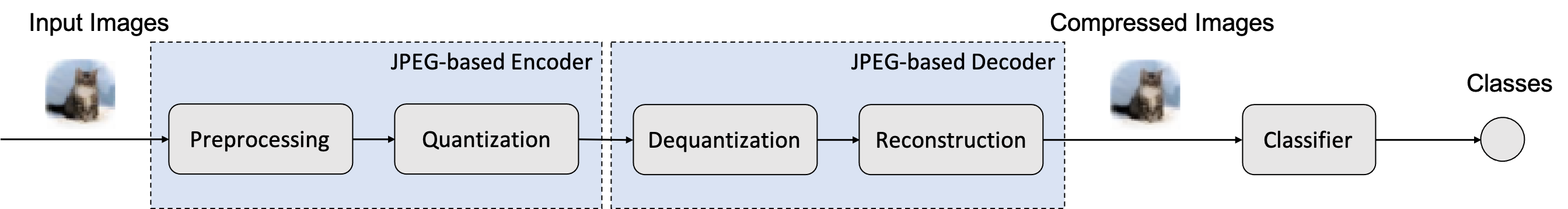
Figure 1: Proposed architecture for CIFAR-100 and Tiny ImageNet. The detailed structure in WRN-28 is omitted here.

III-A1 Compression Layers

The trainable quantization layer in our proposed WRN model is similar to the “quan block” in [11], as shown in Fig. 1. JPEG can take three distinct Q-tables $\boldsymbol{Q}_{1}$, $\boldsymbol{Q}_{2}$, and $\boldsymbol{Q}_{3}$, respectively, for each of the YCBCR color channels, leading to 192 parameters in this layer. Same as [11], we replace the trainable quantization parameters by element-wise reciprocal of the Q-table entries $\boldsymbol{q}_{i}(j,k)=\boldsymbol{Q}_{i}(j,k)^{-1}.$ The matrices $\boldsymbol{q}_{i}$, referred to as the “compression kernels”, allows the model to learn to discard any frequency domain information by setting the corresponding entry $\boldsymbol{q}_{i}(j,k)=0$. Smaller $\boldsymbol{q}_{i}$ values lead to smaller range of quantized DCT coefficients and consequently generates fewer encoded bits.

The quantization layer includes a non-differentiable rounding operation $a(\boldsymbol{F})=\mbox{round}(\boldsymbol{F})$, which cannot be used in a gradient-based training framework, as its activation function. Following [15], we address this problem by substituting a smooth approximation $\hat{a}(\boldsymbol{F})=\boldsymbol{F}$ for the rounding function in backpropagation. Together, preprocessing and quantization layers form a JPEG-based encoder.

The dequantization layer only needs to multiply the encoded DCT blocks $\boldsymbol{F}_{q}$ element-wise by their respective Q-table matrices $\boldsymbol{Q}_{1}$, $\boldsymbol{Q}_{2}$ and $\boldsymbol{Q}_{3}$ corresponding to the encoder quantization layer. The quantization and dequantization layers jointly form a pair of “compression layers”.

III-A2 Reconstruction Layer

As described in Section II, the reconstruction layer performs IDCT via $\boldsymbol{I}=\boldsymbol{D}^{T}\boldsymbol{F}_{q}\boldsymbol{D}$ for each quantized DCT coefficient block $\boldsymbol{F}_{q}$ and rearranges the reconstructed blocks $\boldsymbol{I}$. CB and CR channels are upsampled via bilinear interpolation. The outputs of this layer are YCBCR spatial images. Together, the dequantization layer and the reconstruction layer form the JPEG decoder.

III-A3 Classifier

WRNs[16] achieve impressive classification performance on the CIFAR-100[17] and Tiny ImageNet[18] datasets. Without loss of generality, we adopt a 28-layer WRN as the classifier. For CIFAR-100, we set the convolutional layer width multiplier $k=10$, same as that used in [16]. For Tiny ImageNet, we set $k=1$ to further simplify training.

III-B Loss Function During Training

To jointly reconfigure the JPEG parameters in compression layers and to optimize the deep learning classifier, we design the following loss function during training:

$$\mathcal{L}=\mathcal{L}_{\rm CLA}+\lambda\mathcal{L}_{\rm Quan},\vspace*{-2mm}$$

where $\mathcal{L}_{\rm CLA}$ is the cross entropy classification loss, $\mathcal{L}_{\rm Quan}$ is a penalty term for the compression kernels and $\lambda$ is an adjustable hyper-parameter to govern the importance of the rate. Since there is no simple or standard metric to directly control JPEG encoded image size, which further involves RLE and Huffman coding, we propose the following surrogate penalty function:

$$\mathcal{L}_{\rm Quan}=\sum_{i=1}^{3}\sum_{j=1}^{8}\sum_{k=1}^{8} \left[\mbox{max}(\boldsymbol{q}_{i}^{2}(j,k)-c,0)+\lambda_{1}|\boldsymbol{q}_{i}(j,k)|\right]$$

where $c$ and $\lambda_{1}$ are tunable hyper-parameters. The $\ell_{1}$ loss term promotes sparsity whereas the $\ell_{2}$ loss term regulates the compression kernels. The hyper-parameter $c$ acts as a constraint on the squared magnitude of $\boldsymbol{q}_{i}$, shall be appropriately selected based on the values of $\lambda$ and $\lambda_{1}$. Larger $\lambda$ and $\lambda_{1}$ and a smaller $c$ leads to higher compression ratio and lower classification accuracy. We propose the current form of the surrogate penalty function after testing both logarithm and sigmoid functions without witnessing performance benefits.

III-C Modified ResNet for ImageNet

For ImageNet, we adopt the same preprocessing steps and quantization layer from III-A and utilize the Deconvolution-RFA architecture in [10], which is inspired by ResNet-50, as the classifier. As demonstrated in Fig. 2, the quantized DCT coefficients of CB and CR channels are augmented to the same spatial size as Y channel by two separate transposed convolutional layers. The three channels are concatenated as input of the deconvolution-RFA model. Considering the higher complexity of this model, we suggest a single $\ell_{2}$ regularization for compression kernels for optimizing the quantization parameters via quantization loss $\mathcal{L}_{\rm Quan}=\sum_{i=1}^{3}\sum_{j=1}^{8}\sum_{k=1}^{8}\boldsymbol{q}_{i}^{2}(j,k).$

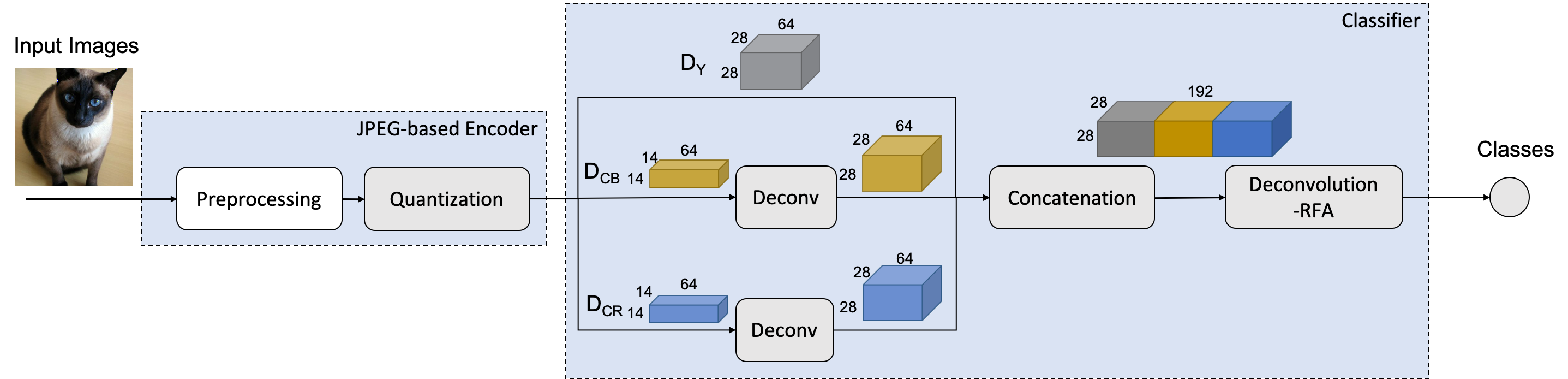
Figure 2: Architecture of our proposed model for ImageNet. The detailed structure of Deconvolution-RFA[10] is omitted here.

III-D Implementation

We test the learning framework in Fig. 1 with CIFAR-100 and Tiny ImageNet datasets. The images in CIFAR-100 dataset are of $32\times 32$ pixels, while images in Tiny ImageNet are of $64\times 64$ pixels.

There are 192 trainable parameters in the compression kernels, all initialized to 1. The randomly-initialized WRN-28 classifier is trained jointly with the parameters in compression kernels, as well as the color transformation coefficients if needed, using Adam optimizer with a batch size of 100. The training of WRN-28 proceeds alternatively: the classifier is trained for 2 epochs while JPEG-based layers are frozen, followed by the compression layer being trained for 1 epoch while freezing the classifier. The training takes 150 such alternations. The learning rate starts from 0.05, and is scaled by 0.1 and 0.01, at alternation 50 and 100, respectively.

We implement the larger learning framework in Fig. 2 with ImageNet in which the images are of $224\times 224$ pixels. Similarly, color transformation coefficients are initialized to JPEG standard and all 192 quantization parameters are initialized to 1. The color transformation, compression kernels, and Deconvolution-RFA classifier are trained from end to end by using Adam optimizer with a batch size of 32. The learning rate of compression kernels starts from $1\times 10^{-8}$ while that for other parameters starts from 0.001. Both learning rates are scaled by 0.1, 0.01, and 0.001, at epoch 30, 60 and 80, respectively. The training takes 90 epochs.

For the quantized DCT coefficients using the new Q-tables, we customize Huffman tables for bandwidth saving by randomly choosing 50k images from the corresponding training set to generate Huffman tables. The bandwidth of the validation data set is measured by combining the principles of RLE and Huffman coding.

IV Experiments

Our experiments are conducted on Keras and TensorFlow. We utilize the two metrics to evaluate perceptual quality of images: peak signal-to-noise ratio (PSNR) and structural similarity index measure (SSIM) index. We test the proposed joint compression and classification (JCC) frameworks on three datasets: (a) CIFAR-100 dataset based on 50k training images and 10k test images belonging to 100 categories; (b) Tiny ImageNet dataset based on 100k training images and 10k validation images belonging to 200 categories; (c) ImageNet dataset based on approximately 1.3M training images and 50k test images belonging to 1000 categories.

IV-A JPEG Standard Baseline

We first present baseline results of images using standard JPEG algorithm with 4:2:0 chroma subsampling. We initialize compression kernels $\boldsymbol{q}_{i}$, $i=1,\ 2,\ 3$ using the Q-tables given in JPEG standard. In this baseline scenario, we only adapt the classifier parameters during training.

For CIFAR-100, we consider 9 different JPEG image qualities between $12.5$% and $100\%$. For Tiny ImageNet, we select 4 different image qualities between $10$% and $80\%$. For ImageNet, our experiments consider 5 different image qualities between $12.5$% and $100\%$. The classification results are shown in Figs. 3-4. These baseline results reveal that the classification accuracy correlates positively with image qualities and average image bandwidth (rate).

IV-B Joint Compression and Classification (JCC)

For JCC, we train and optimize the compression kernels and the classifier. For CIFAR-100, we selected 8 values of $\lambda$ from $10^{-6}$ to $5$ with $\lambda_{1}=1$ and $c=0.01/\lambda$. The classification accuracy, PSNR and SSIM results can be found in Fig. 3. Compared with the JPEG baseline, JCC achieves clear improvement of up to 2.4% in accuracy at bandwidth between 0.75 and 1.5 KB per image. The PSNR and SSIM of JCC-compressed images are similar to those using JPEG.

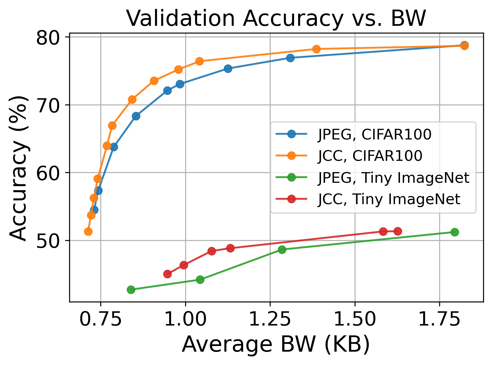
(a)

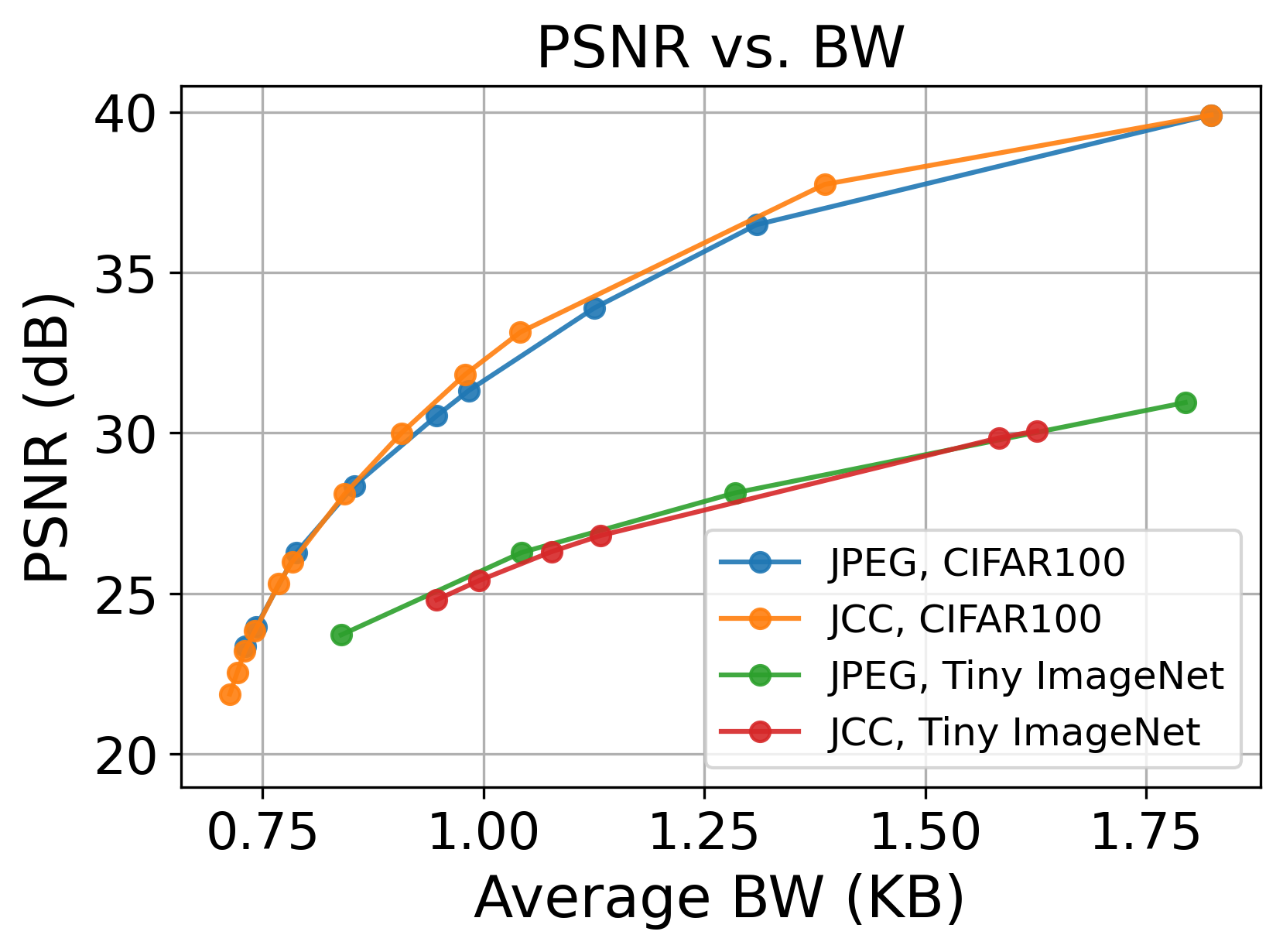
(b)

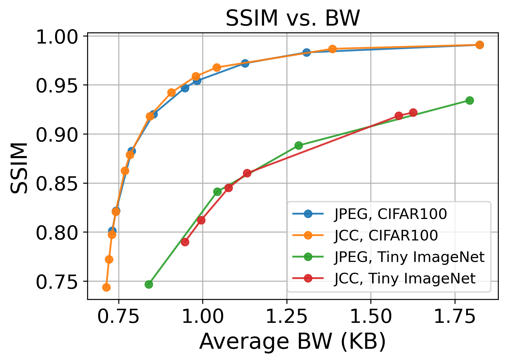
(c)

Figure 3: Comparison between JCC and JPEG standard on CIFAR-100 and Tiny ImageNet datasets with WRN-28 Model, with respect to classification accuracy, PSNR and SSIM versus average bandwidth.

For Tiny ImageNet, we select 6 values of $c$ from $5\times 10^{-3}$ to $0.8$. As shown in Fig. 3, when comparing with the JPEG baseline, we observe accuracy gain of up to 4% by the proposed JCC model at low bandwidth between 0.9 and 1.6 KB per image while maintaining similar visual quality. Overall, the PSNR and SSIM of JCC-optimized and JPEG standard quantization tables are similar.

For ImageNet, we consider 9 values of $\lambda$ between $25$ and $100$. The resulting top-5 classification accuracy, PSNR, and SSIM are given in Fig. 4. For encoding rates below 11 KB per image, the JCC model outperforms the baseline by up to $3.7\%$ in terms of classification accuracy. For bandwidths above 11 KB per image, the classification accuracy difference between JPEG and JCC is quite insignificant. Furthermore, PSNR and SSIM of JCC-compressed images outperform those of standard JPEG encoded images.

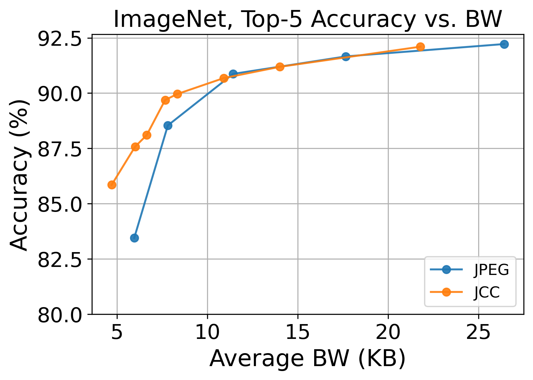
(a)

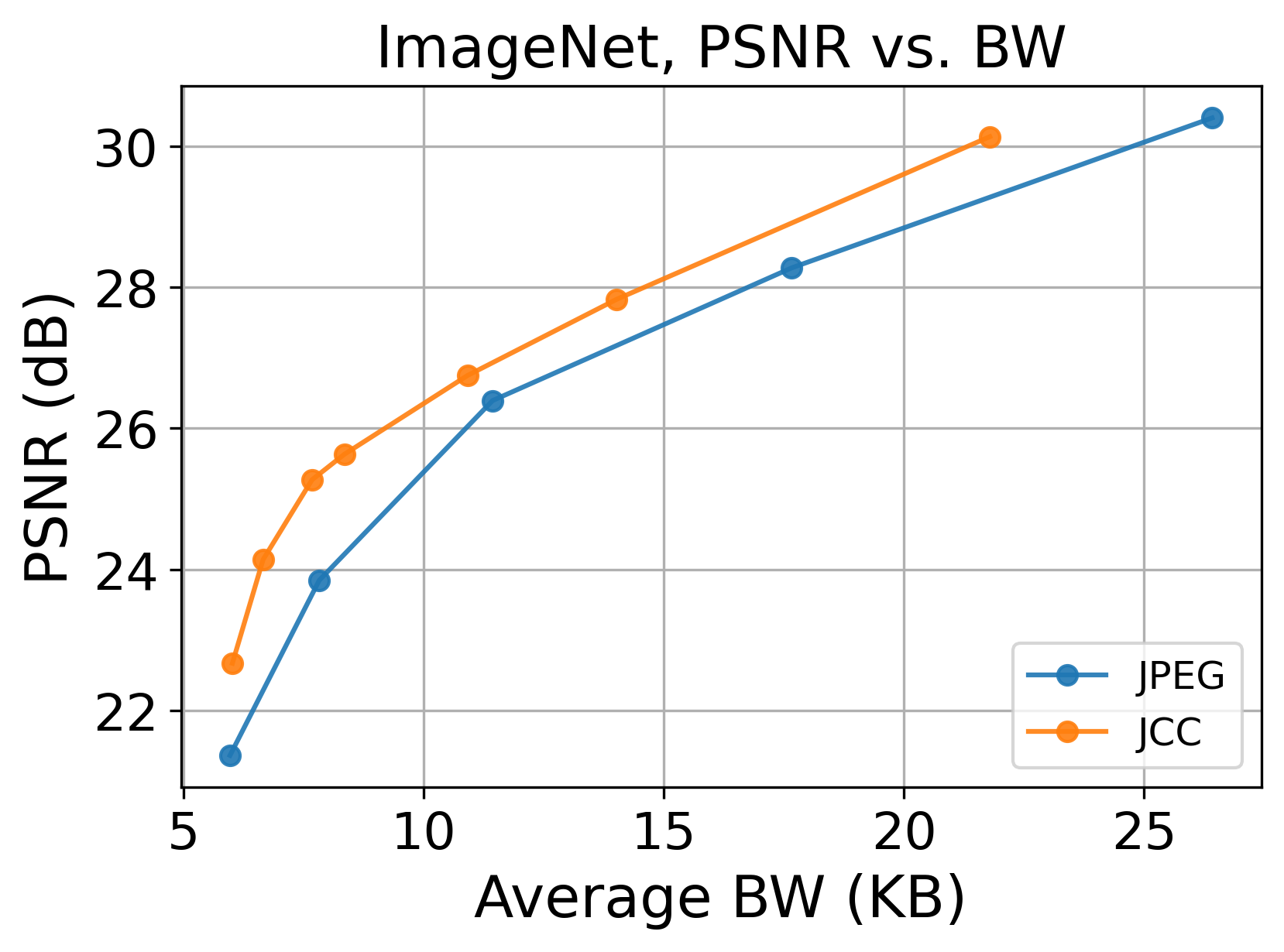
(b)

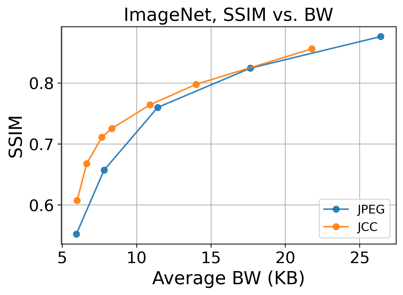
(c)

Figure 4: Comparison between JCC and JPEG baseline on ImageNet dataset with Deconvolution-RFA Model, with respect to top-5 classification accuracy, PSNR and SSIM versus average bandwidth.

From these experimental results, we observe that the JCC model can effectively optimize the JPEG compression kernels for better rate-accuracy trade-off, especially at moderate image bit rates. It is intuitive that the performance edge of JCC diminishes for very high image sizes because most image features can be preserved when given sufficient number of bits and JCC and JPEG no longer need to delicately balance the rate-accuracy trade-off. Similarly, for very low image sizes, very few bits can be used to encode vital information in DCT coefficients. Hence, the encoders have less flexibility to further optimize the rate-accuracy trade-off, thereby making it difficult for even the JCC model to find better parameter settings.

IV-C JCC and Color Transformation

Considering JCC and color transformation (JCC-color), color transformation coefficients, compression kernels and classifier are jointly trained. We initialize the color conversion coefficients according to the settings in JPEG. According to our experimental results, tuning the color transformation coefficients offers no performance gain over JCC. Theoretically, invertible color space transformation does not lead to information loss and can be subsumed by first dense-layer in the neural network. In fact, we observe that the resulting color transform rarely move from their initial values and further optimization is unnecessary.

IV-D Further Analysis and Discussions

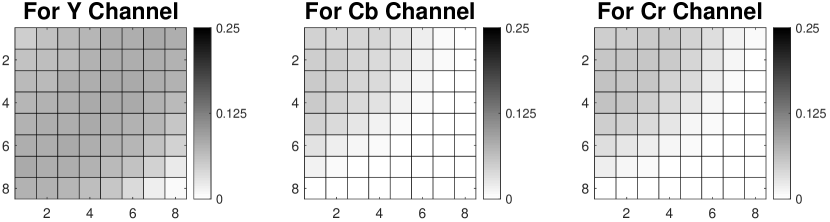
(a)

Figure 5: JCC optimized compression kernels based on CIFAR-100 for Y (left), CB (middle) and CR (right) channels, with $\lambda=0.001,\lambda_{1}=1$ and $c=10$.

Our experimental results suggest that trainable JCC model can extract critical DCT features for classification among categories of CIFAR-100, Tiny ImageNet, and ImageNet datasets. Furthermore, the perceptual quality of images are preserved. Fig. 5 shows the resulting compression kernels with which WRN-28 achieves classification accuracy of 75.20% at an average rate of 0.979 KB/image. Darker grids imply low compression or higher importance of the corresponding DCT coefficient. The encoder clearly favors lower frequency bands. Since there are longer consecutive 0’s in the zig-zag order in the end-to-end learned compression kernels, the correspondingly compressed DCT coefficients require fewer bits via RLE. Furthermore, the trainable model learns to discard some higher frequency DCT components less critical to classification.

Together, these experimental results show performance enhancement on standardized JPEG codec for cloud-based image classification. The optimized Q tables can be distributed in pre-installed JPEG encoders of low-cost devices through software updates for different encoding sizes.

V Conclusions

We present an end-to-end deep learning (DL) architecture to jointly optimize JPEG image compression and classification for low-cost sensors in distributed learning systems. Results on CIFAR-100, Tiny ImageNet, and ImageNet datasets demonstrate successful training of the end-to-end DL framework for better image compression and classification performance without perceptual quality loss. Optimized JPEG Q-tables can be readily incorporated within deployed codecs in practice. Future works may explore the broad appeal of this end-to-end learning principle in other bandwidth-constrained distributed DL tasks such as object detection, segmentation, and tracking.

References

- [1] K. He, X. Zhang, S. Ren, and J. Sun, “Deep residual learning for image recognition,” pp. 770–778, 2016.
- [2] C. R. T.81, “Information technology - Digital compression and coding of continuous-tone still images - Requirements and guidelines.” Standard, 1992.
- [3] S.-W. Wu and A. Gersho, “Rate-constrained picture-adaptive quantization for JPEG baseline coders,” in Int. Conf. on Acoustics, Speech, and Signal Processing. IEEE, 1993, pp. 389–392.
- [4] E. Tuba, M. Tuba, D. Simian, and R. Jovanovic, “JPEG quantization table optimization by guided fireworks algorithm,” in Int. Workshop on Combinatorial Image Analysis. Springer, 2017, pp. 294–307.
- [5] X. Luo, H. Talebi, F. Yang, M. Elad, and P. Milanfar, “The rate-distortion-accuracy tradeoff: JPEG case study,” arXiv:2008.00605, 2020.
- [6] S. Singh, S. Abu-el Haija, N. Johnston, J. Ballé, A. Shrivastava, and G. Toderici, “End-to-end learning of compressible features,” arXiv:2007.11797, 2020.
- [7] L. Theis, W. Shi, A. Cunningham, and F. Huszr, “Lossy image compression with compressive autoencoders,” 2017.
- [8] S. Diamond, V. Sitzmann, S. Boyd, G. Wetzstein, and F. Heide, “Dirty pixels: Optimizing image classification architectures for raw sensor data,” 2017.
- [9] X. Zou, X. Xu, C. Qing, and X. Xing, “High speed deep networks based on discrete cosine transformation,” in IEEE Int. Conf. on Image Proc., 2014, pp. 5921–5925.
- [10] L. Gueguen, A. Sergeev, B. Kadlec, R. Liu, and J. Yosinski, “Faster neural networks straight from JPEG,” in Advances in Neural Information Processing Systems, 2018, pp. 3937–3948.
- [11] L. D. Chamain, S. S. Cheung, and Z. Ding, “Quannet: Joint image compression and classification over channels with limited bandwidth,” in 2019 IEEE Int. Conf. on Multimedia and Expo (ICME), 2019, pp. 338–343.
- [12] Z. Liu, T. Liu, W. Wen, L. Jiang, J. Xu, Y. Wang, and G. Quan, “DeepN-JPEG: A deep neural network favorable JPEG-based image compression framework,” Proc. 55th Annual Design Automation Conf., 2018.
- [13] Z. Li, C. D. Sa, and A. Sampson, “Optimizing JPEG quantization for classification networks,” arXiv:2003.02874, 2020.
- [14] J. Choi and B. Han, “Task-aware quantization network for JPEG image compression,” in European Conf. on Computer Vision. Springer, 2020, pp. 309–324.
- [15] L. Theis, W. Shi, A. Cunningham, and F. Huszár, “Lossy image compression with compressive autoencoders,” arXiv:1703.00395, 2017.
- [16] S. Zagoruyko and N. Komodakis, “Wide residual networks,” arXiv:1605.07146, 2016.
- [17] A. Krizhevsky, “Learning multiple layers of features from tiny images,” Tech. Rep., 2009.
- [18] Y. Le and X. Yang, “Tiny imagenet visual recognition challenge,” CS 231N, vol. 7, 2015.