A Wideband Polarization Observation of Hydra A with the Jansky Very Large Array

Abstract

We present results of a wideband high-resolution polarization study of Hydra A, one of the most luminous FR I radio galaxies known and amongst the most well-studied. The radio emission from this source displays extremely large Faraday rotation measures ($\mathrm{RM}$s), ranging from $-12300$ rad m^-2 to $5000$ rad m^-2, the majority of which are believed to originate from magnetized thermal gas external to the radio tails. The radio emission from both tails strongly depolarizes with decreasing frequency. The depolarization, as a function of wavelength, is commonly non-monotonic, often showing oscillatory behavior, with strongly non-linear rotation of the polarization position angle with $\lambda^{2}$. A simple model, based on the $\mathrm{RM}$ screen derived from the high frequency, high resolution data, predicts the lower frequency depolarization remarkably well. The success of this model indicates the majority of the depolarization can be attributed to fluctuations in the magnetic field on scales $<1500$ pc, suggesting the presence of turbulent magnetic field/electron density structures on sub-kpc scales within a Faraday rotating (FR) medium.

1 Introduction

Hydra A (3C $218$) is a wide-tailed Fanaroff-Riley type I (FR I) radio galaxy. With a spectral luminosity of $P_{178\text{MHz}}=3\times 10^{26}$ W Hz^-1 sr^-1 (Taylor et al., 1990), it is one of the most luminous FRI galaxies known. The radio galaxy is hosted by a cD elliptical galaxy situated at redshift $0.054$ (Dwarakanath et al., 1995; Owen et al., 1995; Taylor, 1996). This galaxy is the dominant member of the relatively poor Abell cluster A780 (Abell, 1958).

At low radio frequencies, Hydra A’s detectable radio structure extends $\sim 530$ kpc in the North-South direction, and $\sim 265$ kpc in the East-West direction (Taylor et al., 1990; Lane et al., 2004). The right panel of Figure 1 shows this large-scale structure at 1.04 GHz with 28$\arcsec$ resolution. The left panel of this figure shows the brighter inner tails and jet emission at 11.1 GHz with 2.65$\arcsec$ resolution, whose polarimetric structures are the subject of this paper. The polarized emission from the outermost parts of the source is too faint to be detected in our observations.

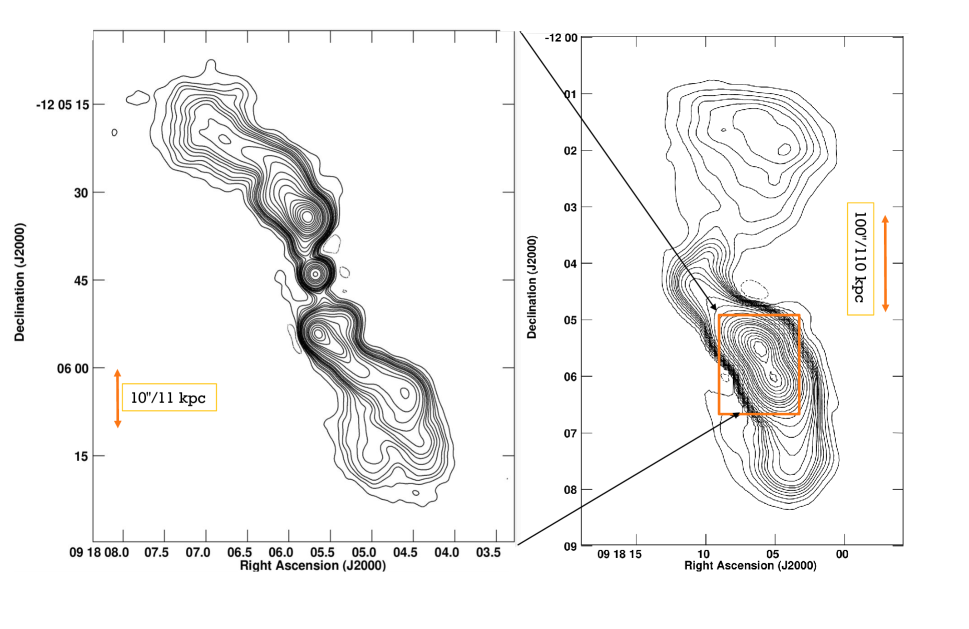
Figure 1: Total intensity contour maps of Hydra A, showing the inner tails (left) and jets at 11.1 GHz with 2.65$\arcsec$ resolution, and the low-brightness extended tails (right) at 1.04 GHz with 28$\arcsec$ resolution. The colored box in the right panel shows the extent of the left panel image. These images are from the VLA Calibrator Monitoring Program observations taken with the VLA in 2013. Left plot: The peak brightness is 0.59 Jy beam^-1 and contour levels are 0.0059$\times$(-0.2, 0.2, 0.5, 0.75, 1, 1.5, 2, 2.5, 3, 4, 5, 7.5, 10, 15, 20, 25, 30, 40, 50, 60, 70, 80, 90) Jy beam^-1. Right plot: The peak brightness is 20.1 Jy beam^-1 and contour levels are 0.0201$\times$(-0.1, 0.1, 0.2, 0.3, 0.4, 0.5, 0.6, 0.8, 1, 1.25, 1.5, 2, 3, 5, 7.5, 10, 15, 20, 25, 30, 35, 40, 50, 60, 70, 80, 90) Jy beam^-1.

Hydra A is embedded in a cool core X-ray cluster of luminosity $L=4\times 10^{44}$ ergs s^-1 between $0.5$ and $4.5$ keV (David et al., 1990). The cluster gas temperature decreases from roughly $4$ keV at $200$ kpc radius to $3$ keV at $10$ kpc (McNamara et al., 2000; David et al., 2001), while the electron density, $n_{e}$, within 10 kpc is $0.06$ cm^-3 (McNamara et al., 2000), and decreases with radius as $r^{-0.4}$ out to $30$ kpc, and as $r^{-1.6}$ out to $100$ kpc (David et al., 2001).

X-ray deficit regions are found coincident with the radio tails (McNamara et al., 2000; David et al., 2001; Nulsen et al., 2002). These are most obvious on X-ray maps superimposed by radio intensity at $330$ MHz, see Figures 1 and 2 of Simionescu et al. (2009), and Figure 2 of Nulsen et al. (2005). Such regions – commonly referred to ‘cavities’ – are common in clusters of galaxies hosting radio galaxies, (e.g Boehringer et al., 1993; Carilli et al., 1994; Fabian et al., 2000; Blanton et al., 2001; Heinz et al., 2002), and are believed to result from exclusion of the thermal cluster gas by the expanding bubble of synchrotron-emitting relativistic gas originating from the nucleus. Surrounding the cavities is a region of enhanced X-ray surface brightness gas and pressure (Nulsen et al., 2005; Simionescu et al., 2009). For Hydra A, this enhanced region extends $6\arcmin$ north and $4.3\arcmin$ east of the AGN (Nulsen et al., 2005). This enhancement is interpreted as weak shocks of Mach number $\sim 1.3$ due to the same energy outburst from the nucleus that created the current radio source (Simionescu et al., 2009). Similar weak shocks are also observed in the Perseus cluster (Fabian et al., 2003), M87 (Young et al., 2002) and Cygnus A (Snios et al., 2018).

The radio emission from Hydra A displays extremely large Faraday rotation measures ($\mathrm{RM}$), with the northern tail showing $\mathrm{RM}$s ranging from $-1000$ and $+3300$ rad m^-2, and the southern tail showing $\mathrm{RM}$s from a few $\times 1000$ rad m^-2 down to $-12000$ rad m^-2 (Taylor et al., 1990; Taylor & Perley, 1993). The rotation measures are predominantly positive in the northern tail, and predominantly negative and patchy in the southern tail (Taylor & Perley, 1993). Large rotation measure gradients are also observed in both tails, with gradients of up to $\sim 1000$ rad m^-2 arcsec^-1 in the northern tail, and much larger values in the southern tail (Taylor & Perley, 1993). Additionally, the southern tail is less polarized compared to the northern tail, and depolarizes much more rapidly with frequency (Taylor & Perley, 1993). The $\mathrm{RM}$ maps of Hydra A were also statistically analyzed by Vogt & Enßlin (2005) and Kuchar & Enßlin (2011) for the underlying magnetic power spectra, and the Kolmogorof like spectra were reported.

Taylor et al. (1990) attributed the observed depolarization in the tails to the large transverse gradients in $\mathrm{RM}$ rotating the intrinsic source polarization by more than 1 radian over the angular scale of the resolution beam.

The large $\mathrm{RM}$ can be due to the ambient cluster gas, or a boundary layer of compressed cluster gas surrounding the tails, or a region of mixed synchrotron gas with external thermal gas in the boundary layer. Using the most recent RM reconstructed map from Hutschenreuter et al. (2022), we estimate the RM contribution from our Galaxy in the direction of Hydra A to be $-1.038\pm 9.639$ rad m^-2, derived over 5 deg radius – suggesting that our Galaxy cannot account for the observed RMs and gradients. Finally, the optical line emitting gas observed by Baum et al. (1988) extends only to a radius of $15\arcsec$ from the nucleus, and hence cannot account for the overall large-scale high $\mathrm{RM}$s across the tails.

Taylor & Perley (1993) argued against internal Faraday rotations based on three observables: the lack of correlation between the observed $\mathrm{RM}$s with the depolarization; the similarity in $\mathrm{RM}$s across the tails and jets would imply that the internal mixing occurs equally in these regions – but this is unlikely since they are intrinsically different; and the absence of non-linearities in position angle vs. $\lambda^{2}$ which are expected for rotations $>90^{\circ}$. On the other hand, the asymmetries in the $\mathrm{RM}$ distribution between the tails is explained using the Laing-Garrington effect originating from a medium of size $\lesssim 2\times$ the source (Laing, 1988; Garrington et al., 1991). Taylor & Perley (1993) estimated a source inclination to the sky plane of $\leq 60^{\circ}$.

Most, if not all, depolarization mechanisms will not produce a perfectly linear relation between the observed electric vector and $\lambda^{2}$. The physical details of the depolarization process will be contained in these non-linearities, along with the detailed decline of the polarization fraction. The study by Taylor & Perley (1993) consisted of only five wavelengths spanning $2$ to $3.6$ cm. With such sparse sampling, subtle depolarization effects, such as those due to turbulent small-scale magnetic fields or to boundary layer effects will not be visible. Additionally, the depolarization effects, which are most manifest at long wavelengths, may not be seen at such short wavelengths. With the availability of the wideband Jansky Very Large Array (JVLA, Perley et al., 2001), we have the capability to observe Hydra A at lower frequencies than those available to Taylor et al. (1990); Taylor & Perley (1993), – notably, with the $2$ – $4$ GHz system – and with complete frequency coverage, thus allowing a detailed study of the depolarization characteristics of the source.

In this paper, we present a full polarization study of Hydra A using the wideband ($2$ – $12$ GHz) capabilities of the JVLA. The data have unprecedented high sensitivity and high spectral resolution. Our goals are to better determine the polarization structures of the jets and tails, to accurately determine the depolarization characteristics, and to determine the characteristics of the magnetic field structures likely responsible for the extraordinary depolarization.

This paper is organized as follows: The observations and calibration of the data are presented in Section 2, and the imaging of the data in Section 3. Section 4 presents our polarization results, followed by the results of a high-frequency high-resolution Faraday rotation study in section 5. In section 6 we show the results of applying the high frequency, high resolution model to the low frequency data. A summary is presented in Section 7.

2 Observations and Data Calibration

Hydra A was observed in all four VLA configurations under project code 13B-088 at L (1 - 2 GHz), S (2 - 4 GHz), C (4 - 8 GHz), and X (8 - 12 GHz) band resulting in a total frequency coverage of $1$ - $12$ GHz. The observing dates, durations and configurations are shown in Table 1. All bands (L, S, C, and X) were observed together.

Table 1: Observing log.

Array	Observation	Duration
configuration	date	[hr]
B	2013 Dec 14	$6.0$
A	2014 Feb 27	$5.0$
A	2014 Mar 07	$5.0$
D	2014 Jun 27	$4.0$
C	2014 Oct 19	$4.0$

The data were taken with a time resolution of 2 seconds in A-configuration, and 3 seconds in other configurations. The frequency channelization varied with band and configuration: 2 MHz for S-, C- and X-bands in B, C, and D configuration, 1 MHz for L-band in those same configurations. For A configuration, 2 MHz was used for X-band, 1 MHz for C-band, 0.5 MHz for S-band, and 0.25 MHz for L-band. These data were subsequently resampled to the same spectral resolution as in the B, C and D configurations using the AIPS program SPEC. This resulted in a spectral resolution of 1 MHz in L-band, and 2 MHz in the other bands. These values were chosen so as to minimize both the bandwidth smearing and bandwidth depolarization.

All calibration and imaging of the data were done using the Astronomical Image Processing System (AIPS) software (Greisen, 1990; van Moorsel et al., 1996).

The editing and calibration procedures were exactly the same as for Cygnus A (see Sebokolodi et al., 2020, for details). After calibration, the data were averaged in frequency and time to: 1 MHz/12 seconds for L-band, 2 MHz/12 seconds for S-Low (2 - 3 GHz), 4 MHz/12 seconds for S-Hi (3 - 4 GHz), and 8 MHz/12 seconds for C- and X-band.

As the original external phase and amplitude calibration is not sufficiently accurate to enable high-fidelity imaging, self-calibration of the Hydra A data was performed to remove gain drifts between the individual spectral windows due to time-variable changes in bandpass shape, and between the data taken in the four separate configurations. For this purpose, we utilized the emission from the bright, unresolved nucleus to put all the data on a common flux density and positional scale. We achieved this by using the long spacings to phase/amplitude reference the shorter ones. This was done by making an A-configuration-only image, and self-calibrating the data from that model. Once this was done, we use the improved image to self-calibrate the “B” configuration, then adding those data to the “A” data, and making a model using both. Then repeat this with C and D configurations, extending the short-spacing limit downwards each time to ensure stable solutions.

3 Imaging and Data Products

Following the self-calibration process, we made cube images of Stokes $Q$, $U$, and $I$ using a single scale cleaning algorithm. The spatial extent of these image cubes is $4$k by $4$k, sampled with pixel size of $0.05\arcsec$. The cubes were made at two standard resolutions, namely: $1.50\arcsec\times 1.0\arcsec$ and $0.50\arcsec\times 0.35\arcsec$. The lower resolution includes data between 2 - 12 GHz, and the higher includes data between 6 - 12 GHz. The L-band data (1 – 2 GHz) were not utilized in this study, as the depolarization at these frequencies at our resolution of 2 – 3 arcseconds was nearly total.

A false-color rendition of the inner regions of the source at 2.05 GHz, with $1.5\arcsec\times 1.0\arcsec$ resolution is shown in Figure 2. This figure shows the ‘S’ symmetry of the jets and the inner tails. The southern lobe shows a diffuse hotspot a few kpc from the nucleus, while the northern lobe has no discernable hotspot (Taylor et al., 1990).

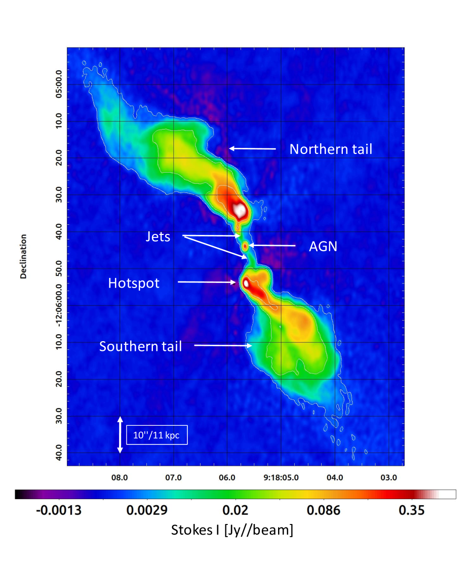
Figure 2: False-color total intensity map at 2.051 GHz with $1.5\arcsec\times 1.0\arcsec$ resolution, showing the inner jets and tails more clearly. This image utilizes data taken for this paper.

To maximize image sensitivity, we combined spectral channels during imaging. However, bandwidth depolarization affects the number of channels we can average together, which depends on the channel frequency and the maximum $\mathrm{RM}$ present in the data. The number of channels $N_{\mathrm{avg}}$ to average together was set by the requirement that the rotation of the plane of polarized emission due to an $\mathrm{RM}$ of 12000 rad m^-2 be less than 10 degrees. Table 2 shows the channelization utilized for the different bands.

Table 2: The number of frequency planes in each band utilized to avoid Faraday depolarization.

Band	$\nu$-interval	$\Delta\nu$	$N_{\mathrm{avg}}$	$N_{\mathrm{planes}}$
	[GHz]	[MHz]
$\mathrm{S_{lo}}$	2-3	2	1	512
$\mathrm{S_{hi}}$	3-4	4	1	256
$\mathrm{C_{lo}}$	4-6	8	1	256
$\mathrm{C_{hi}}$	6-8	16	2	128
$\mathrm{X_{lo}}$	8-10	32	4	64
$\mathrm{X_{hi}}$	10-12	64	8	32

We used single-scale CLEAN because of its speed. However, the accuracy of single-scale deconvolution by CLEAN degrades at high frequencies and high resolutions, particularly for extended emission such as the tails of Hydra A. The problem is particularly severe in Stokes $I$, where the brightness of the extended regions is often broken by CLEAN into synthesized beam-sized ‘islands’ of emission. To reduce these effects, we fitted a smooth brightness profile for each spatial position through the frequency axis of the cube, and used the smoothed value to estimate the Stokes $I$ emission for each frequency plane. This was done separately for the lower-resolution $2$ - $6$ GHz and higher-resolution $6$ - $12$ GHz cubes to avoid significant errors resulting from steepining of spectra at higher frequencies (Cotton et al., 2009). The polarized emission cubes ($Q$ and $U$) do not suffer from this problem, as the high $\mathrm{RM}$ results in these images being dominated by rapidly varying brightnesses which are efficiently and effectively handled by CLEAN.

The off-source noise in the Stokes $Q$ and $U$ images at $0.50$″$\times$ $0.35$″ranges between $0.035$ mJy beam^-1 and $0.12$ mJy beam^-1, and in Stokes $I$ between $0.04$ mJy beam^-1 and $0.3$ mJy beam^-1. At $1.50$″$\times$ $1.0$″, the off-source noise ranges between $0.06$ mJy beam^-1 and 1.1 mJy beam^-1 for Stokes $Q$ and $U$ images, and $0.1$ mJy beam^-1 and $5$ mJy beam^-1 for Stokes $I$ images.

From the Q and U images, we derived the polarized intensity image $P=\sqrt{Q^{2}+U^{2}}$, corrected for Ricean bias, and the polarization angle $\chi=0.5\arctan{U/Q}$, and their associated errors as described in Sebokolodi et al. (2020). We also compute depolarization ratios by taking the ratio of two fractional polarization maps at two different frequencies or resolutions. We estimate the errors in the depolarization ratio map by computing the propagation of error of the two fractional polarization maps.

Additionally, we calculate the Faraday spectra for every line-of-sight using the RM-synthesis technique as described in Sebokolodi et al. (2020). For a more complete description, see the original work by Brentjens & de Bruyn (2005). The rotation measure transfer function for our $2-12$ GHz data has width $\sim$180 rad m^-2, while for the $6-12$ GHz data it is $\sim 2030$ rad m^-2. The computed Faraday spectra were deconvolved using the AIPS task ‘TARS’.

4 Polarization Results

In this section, we analyze the polarization data of Hydra A in detail. In particular, we determine how the polarization changes with frequency and with resolution. This is essential since the depolarization can occur due to differential rotation of the emitting gas, due to magnetized thermal gas along the line-of-sight (“true” or “internal” depolarization), or within our synthesized beam due to unresolved polarization structures (“beam” depolarization). Distinguishing between these phenomena is difficult, but is necessary to have a clear understanding of both phenomena if we are to fully understand the underlying physics associated with radio galaxies.

4.1 Polarization as a Function of Frequency

4.1.1 Fractional Polarization Maps

Figure 3 shows the fractional polarization maps across the tails of Hydra A at $1.5\arcsec\times 1.0\arcsec$ resolution. The northern tail is more polarized than the southern tail at all frequencies. The fractional polarization of both tails decreases with decreasing frequency. The inner regions of the tails close to the nucleus depolarize more rapidly than the outer regions. Similarly to Cygnus A (Sebokolodi et al., 2020), the notable structural features seen in the Stokes ‘$I$’ image, such as the hotspot and jets, are not discernable in the fractional polarization maps. The fractional polarization is relatively smooth across the northern tail, and patchier across the southern tail. However, the fractional polarization of both tails becomes clumpy at low frequencies.

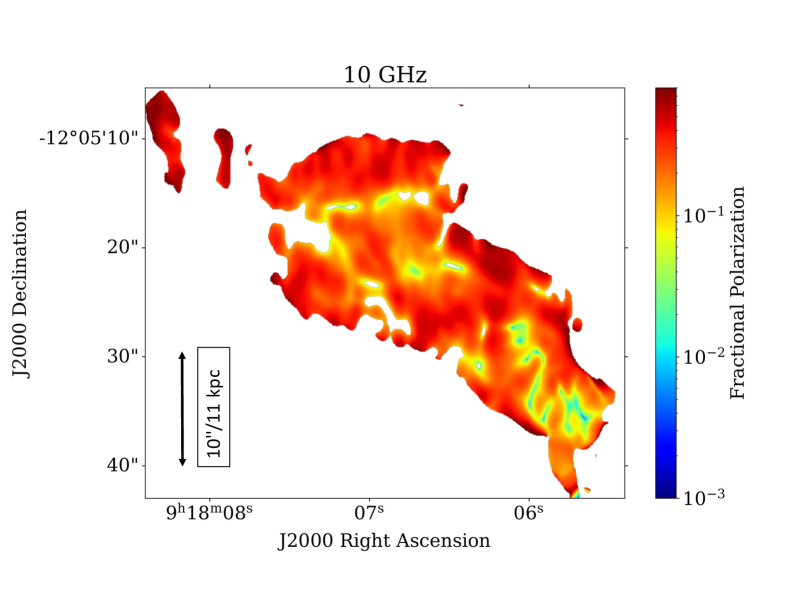
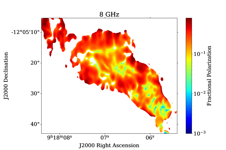
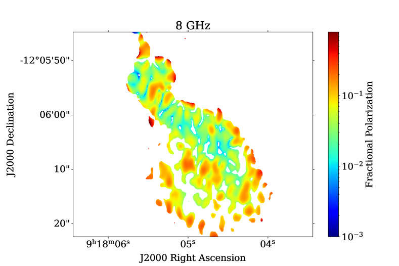
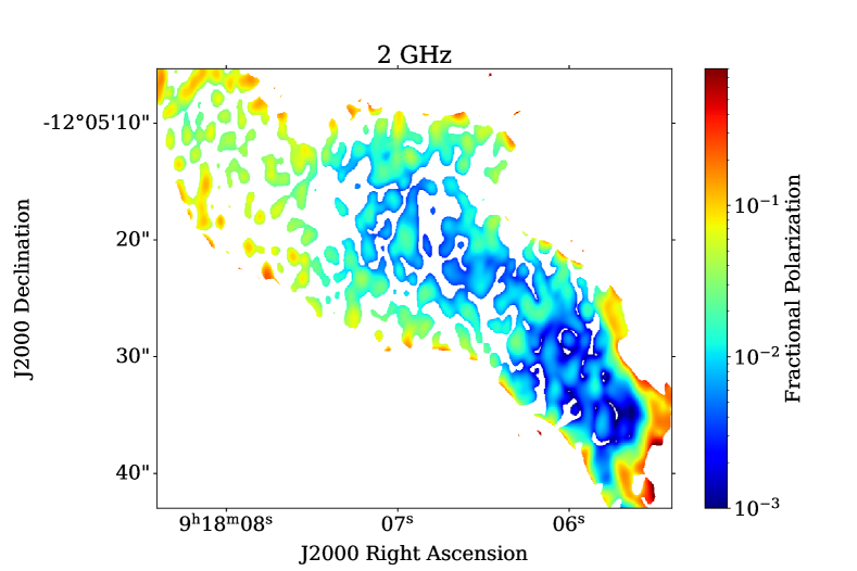
Figure 3: The fractional polarization $p$ across the tails of Hydra A at selected frequencies at a resolution of $1.5\arcsec\times 1\arcsec$. Pixels shown have SNR in $p/\sigma_{p}>60\%$, where $\sigma_{p}$ is the estimated rms noise in the polarization. Left: Northern tail. Right: Southern tail. Both tails depolarize significantly with decreasing frequency. The northern tail is relatively less depolarized compared to the southern tail. The physical scale shown in the top panel is the same for the rest of the panels.

4.1.2 Frequency-Dependent Depolarization Ratio (FDR)

In order to determine the degree by which the tails depolarize, we computed the depolarization ratio by dividing the $1.5\arcsec\times 1.0\arcsec$ resolution fractional polarization map at 2 GHz by the map at 10 GHz (hereinafter FDR1) and 6 GHz by the same 10 GHz map (hereinafter FDR2). The spatial distribution of FDR1 and FDR2 across the tails is shown in Figure 4. Lower values mean stronger depolarization at low frequencies.

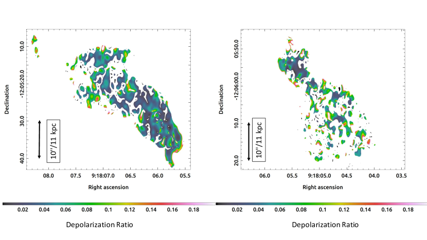
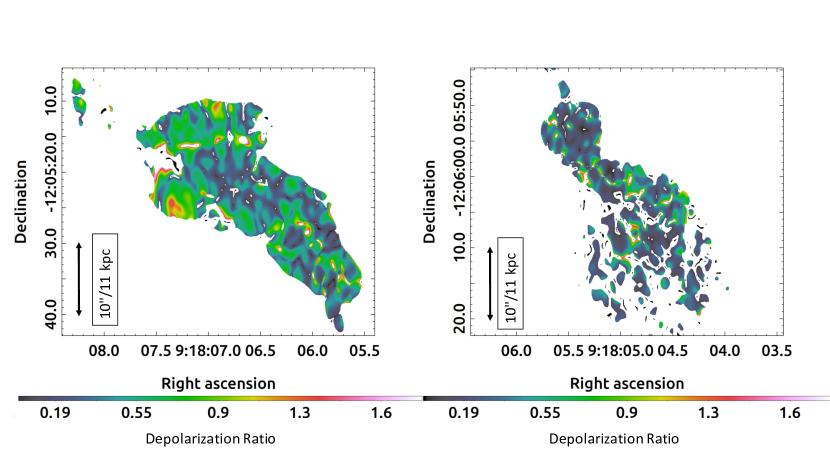
Figure 4: Depolarization ratio maps across the tails at $1.5\arcsec\times 1.0\arcsec$ resolution. Top panel: FDR1 – the ratio of the 2 GHz polarization image to the 10 GHz polarization image. Bottom panel: FDR2 – the ratio of the 6 GHz polarization image to the 10 GHz polarization image. Left panel: Northern tail. Right panel: Southern tail. Only pixels with fractional error of less than $80\%$ are shown. Note the range of color scales in the upper and lower panels are different, due to the stronger depolarization at 2 GHz. Attempting to match the color scales hides the important variations.

The resulting depolarization radial profiles are presented in Figure 5. Due to the shape of the source, it is difficult to orient the source specifically along its extension, so to compute the profiles, we binned the image in slices along right ascension (RA) and declination axis and considered ratios within each bin. The plotted points in the top panel are an average of the depolarization ratios within bins of $2.5^{\prime\prime}$ sizes as a function of declination for all RA within a bin, with zero defined as the location of the nucleus. The bottom plot is the depolarization ratio as a function of right ascension for all declination within a bin. The southern tail is to the left and the northern tail to the right of the AGN in the plot. The spread shown by the shading corresponds to the standard deviation of the ratios within each bin at a given declination/right ascension. The depolarization ratio is prone to large errors since it is a ratio of ratios, so in an attempt to reduce spurious emission we included only those pixels with fractional error in the depolarization ratio less than 80%.

The FDR1 (lower frequency ratio) shows significantly stronger depolarization than the higher frequency ratio, FDR2. The depolarization for FDR1 is $\lesssim 0.1$, and ranges between $0.2-0.8$ for FDR2. This implies that the emission at 10 GHz is depolarized by more than $90\%$ at 2 GHz at this resolution across the tails. In the case of FDR2, there is no significant trend in either depolarization ratio with offset from the nucleus except for the radial increase in the ratio across the northern tail as shown in the bottom plot. In general, the northern tail shows large depolarization values than the southern (i.e., the depolarization is less) – implying a more rapid depolarization across the southern tail relative to the northern tail. Moreover, based on FDR2, the different regions of the tail depolarize widely as suggested by the spread in the distribution.

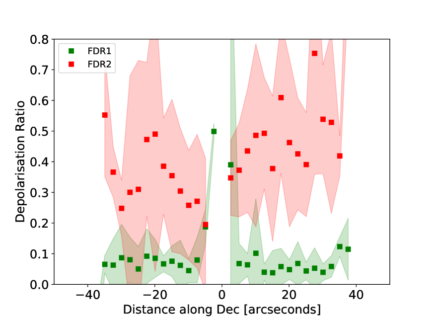
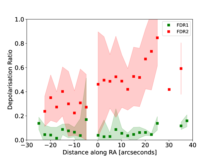
Figure 5: Average frequency depolarization ratios in bins of 2.5″along RA or declination axis. Top: Ratios as a function of declination for all RA. Bottom: Ratios as a function RA for all declination. The southern tail is to the left of RA/Dec $=0^{\prime\prime}$, and the northern tail to the right. Red: Ratio of 6 and 10 GHz denoted as FDR2. Green: Ratio of 2 and 10 GHz (FDR1). Only pixels with fractional error $<80\%$ were used for computing the averages and dispersions. The spread shown corresponds to the standard deviation of the depolarization ratios within bins along declination/RA. The tails depolarize to a similar value for FDR1 ranging between $0.01-0.1$. The distribution of FDR2 shows radial dependence particularly along RA, with a large spread suggesting varying level of depolarization in this higher frequency ratio.

4.1.3 Depolarization vs Wavelength Behavior

We now look at the polarization behavior as a function of $\lambda^{2}$ for different lines-of-sight across our wideband, high-spectral resolution data. This is a lengthy process, due to the large number of lines-of-sight available. For the purpose of this paper, we will show a few ‘representative’ example lines-of-sight.

We first define a relative coordinate system, centered on the galaxy nucleus, with units in tens of milliarcseconds. In this system, north and west are positive, and east and south are negative. Thus, a pixel with coordinate (1585, -3100) is located 15.85$\arcsec$ west, and 31.00$\arcsec$ south of the nucleus. To select our lines-of-sight, we considered pixels separated by 0.7$\arcsec$ with fractional polarization above $0.1$ at $8$ GHz. These choices were motivated by obtaining lines-of-sight that are of good signal-to-noise and are usable for scientific analysis. With these restrictions, we obtain a total of 696 lines-of-sight. However, only 553 of these are considered for further analysis, as the remaining 134 lines-of-sight are too noisy to be used for meaningful analysis. The majority of the excluded lines-of-sight are from the southern tail, and the outermost regions of the tail.

Figure 6 shows the depolarization functions for six representative lines-of-sight. For each line-of-sight (each row) we display fractional polarization as a function of $\lambda^{2}$ (left), polarization angle as a function of $\lambda^{2}$ (middle) and the amplitude of the deconvolved Faraday spectrum (right) superimposed with a real-valued Gaussian of width equal to the full width half maximum of the rotation measure transfer function (in red). To match the Gaussian function to the data, we shifted and scaled its location and amplitude to that of the peak in the Faraday spectrum. Each line-of-sight is labelled using the derived coordinate system.

The fractional polarizations for all 553 lines-of-sight decrease significantly with increasing $\lambda^{2}$. The decline in fractional polarization is commonly non-monotomic, with many lines-of-sight showing sinc-like, or more complicated behavior, as shown in the figure (based on visual inspection). Example lines-of-sight with a relatively smooth decay are shown in the top two rows, those with well-defined oscillations in the third and fourth rows, and those with an intermediate,or more complicated decay, in the last two rows. Hereon we refer to these decay behaviors as “smooth”, “sinc-like”, and “complex” decay, respectively. We find that roughly 22% of the lines-of-sight show smooth decay, 11% sinc-like, and 67% are complex. The sinc-like and more complex decays in fractional polarization generally arise from having more than one $\mathrm{RM}$ value within a single observing beam. For instance, the sinc-like decays might occur due to two similarly strong polarized patches with different $\mathrm{RM}$s within the beam, if each patch itself carries a range of RM values (perhaps due to internal variations in the structure causing the RM patch). A detailed treatment will be presented in Baidoo, Eilek & Perley (in preparation).

The middle column shows the observed polarization angles as a function of $\lambda^{2}$ in black, and the residual polarization angle in blue. Note the different vertical scales for these. The residual angles were obtained by removing the dominant (peak) component in the Faraday spectrum (right panel) as $\chi-RM_{\text{peak}}\lambda^{2}$. There are significant deviations from linearity for most lines-of-sight. These deviations are most prominent at low frequencies – as expected, since the depolarization effects are dominant at this frequency-regime, while linearity is generally observed at high frequencies.

The observed Faraday spectra often reveal very interesting structures (right panel of Figure 6). In general, the Faraday spectra of the smoothly decaying lines-of-sight are relatively less complicated – a single dominant peak, and some cases with broadened spectra with respect to the RMTF, while the sinc-like and complex decaying lines-of-sight have complicated spectra. In particular, the latter two classes have broad Faraday spectra that generally consist of isolated, well resolved peaks (that is, structures separated by more than our $180$ rad m^-2 resolution). The peak separations, or broadening, ranges from a few $\sim 500$ rad m^-2 up to $\lesssim$ 5000 rad m^-2 – with the majority of the large peak separations spanning between 1000 rad m^-2 and 3000 rad m^-2. Complex Faraday structures are also found in wideband polarization studies of other sources, such as O’Sullivan et al. (2012); Anderson et al. (2016); Ma et al. (2019); Riseley et al. (2020); Stuardi et al. (2020), however, those presented in this study and in Sebokolodi et al. (2020) have been observed over a wider range of frequency, allowing a more detailed analysis.

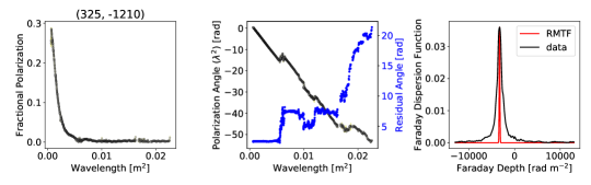
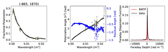
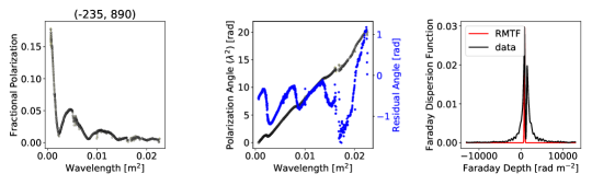
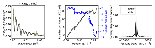
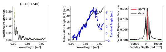
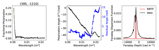
Figure 6: Example lines-of-sight showing fractional polarization vs. $\lambda^{2}$ (left column), the observed polarization angle vs. $\lambda^{2}$ in black and the residual angles in blue (middle column), and Faraday spectra superimposed with the Gaussian RMTF in red (right) all at $1.50\arcsec\times 1\arcsec$. The residual polarization angles were obtained by removing the dominant peak in the Faraday spectrum (subtracting $RM_{\text{peak}}\lambda^{2}$). The top two rows are from the ‘smoothely decaying’ class, the middle two rows from the ‘sinc-like’ class, and the bottom two from the ‘complex class’.

4.2 Polarization as a Function of Resolution

The depolarization can be a result of differential rotation along the line-of-sight (synchrotron-emitting gas mixed with magnetized thermal gas) or across the synthesized beam (beam depolarization, due to unresolved transverse structures in the emission or a foreground screen). These two forms of depolarization have completely different physical implications, but often similar depolarization characteristics. The only definitive way to distinguish between the two is to eliminate beam depolarization by increasing our resolution until all transverse variations are resolved out. Any remaining depolarization can then be attributed to the line-of-sight effect. In this section, we investigate whether our data are limited by the observation’s resolution.

4.2.1 Fractional Polarization Images as a Function of Resolution

Figure 7 shows a 6 GHz fractional polarization map at four different resolutions between 3^′′ and 0.5$\arcsec$ (the latter being the highest we can obtain at this frequency). The tails depolarize with lower resolution, with the largest depolarization occurring in the inner regions of the tails close to the center (most evident across the northern tail).

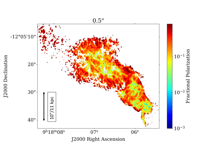
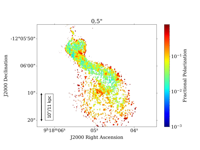
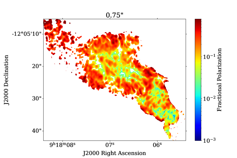
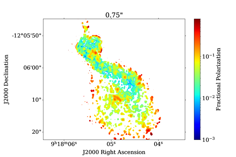
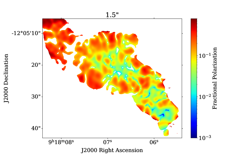
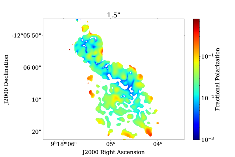
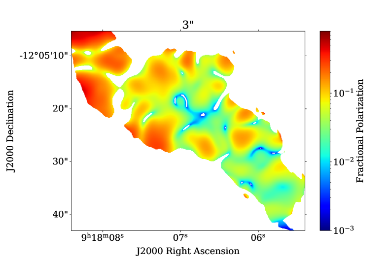
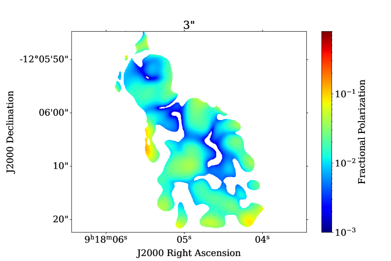
Figure 7: Fractional polarization at $6$ GHz at four resolutions. Left: northern tail. Right: southern tail. Resolution from top to bottom: 0.5″, 0.75″, 1.5″, and 3″. Only pixels with SNR $p/\sigma_{p}>60\%$ are shown. In nearly all locations, the higher resolution images are more highly polarized. The physical scale shown in the top panel is the same for the rest of the panels.

4.2.2 Resolution-Dependent Depolarization Ratio (RDR)

To see the degree by which the tails depolarize as a function of resolution, we computed a depolarization ratio map by dividing the 10 GHz fractional polarization maps at 3$\arcsec$ with the maps of same frequency at 0.3$\arcsec$ (hereinafter RDR1), and 6 GHz fractional polarization maps at 3$\arcsec$ with 0.5$\arcsec$ (hereinafter RDR2).

Figure 8 shows the spatial distribution of RDR across the tails.

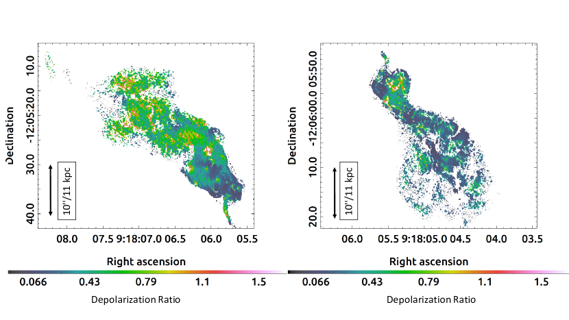
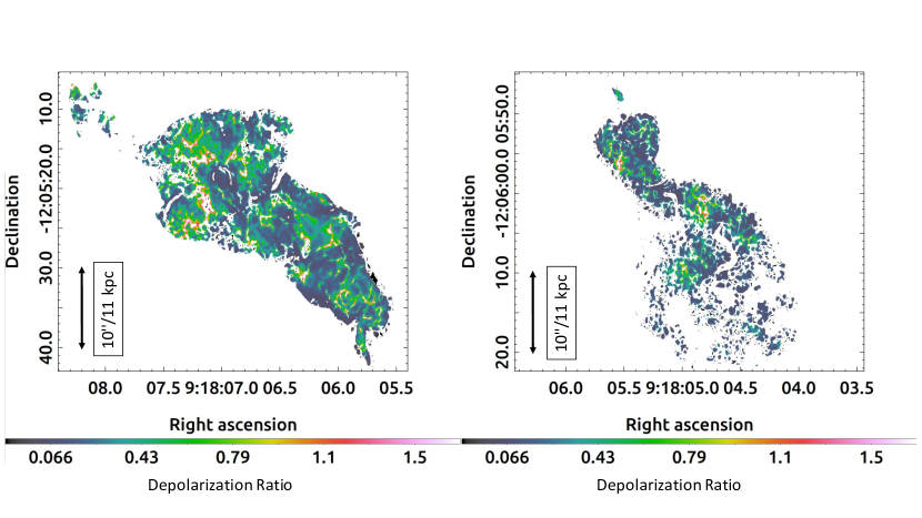
Figure 8: Depolarization ratio maps across the tails. Top panel: RDR1 – the ratio of the 3$\arcsec$ resolution fractional polarization image to the 0.3$\arcsec$ image at 10 GHz. Bottom panel: RDR2 – the ratio of the 3$\arcsec$ fractional polarization to the 0.5$\arcsec$ polarization image at 6 GHz. Only pixels with fractional error of less than $80\%$ are shown.

The corresponding radial profiles are presented in Figure 9 (similar to FDR profiles shown in Figure 5). We utilized only those pixels with fractional error of less than $80\%$ to compute the profiles. The general depolarization ratio behavior is similar at the two frequencies. The two tails depolarize differently with distance from the center: the depolarization across the northern tail decreases with distance from the AGN, while the depolarization is strongest away from the center across the southern tail. Similarly to the frequency-dependent depolarization ratios, the resolution-dependent depolarization is much stronger in the southern tail (left side of declination=$0^{\prime\prime}$). The same behavior is observed for RDR as a function of distance along right ascension.

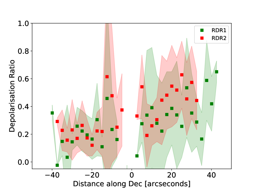
Figure 9: Resolution-dependent depolarization ratio. RDR1 is $3\arcsec/0.30\arcsec$ at 10 GHz. RDR2 is $3\arcsec/0.50\arcsec$ at 6 GHz. The left side of declination zero is the southern tail, and the right side is the northern tail. Pixels shown have fractional error $<80\%$. The general depolarization ratio behavior is similar at the two frequencies. The depolarization is stronger across the southern tail. The two tails depolarize differently with distance from the center: the depolarization across the northern tail decreases with distance from the AGN, while the depolarization is strongest away from the center across the southern tail. We find the same behavior for RDR binned along RA.

4.2.3 Lines-of-Sight Depolarization

As noted earlier, in the presence of small-scale transverse fluctuations, the observed fractional polarization should increase (usually) monotonically with increasing resolution, until reaching a resolution which resolves the foreground fluctuations in the depolarizing screen. At this resolution, the observed fractional polarization will be that of the source itself. If this intrinsic value can be established, any fractional polarization changes with frequency must then be due to intermixed thermal and synchrotron gas of the source, or an intermixed boundary layer, allowing an estimate of the thermal gas content. This is the only means of definitively separating beam-depolarization effects from the more physically relevant depolarization mechanisms.

In Figure 10, we show plots of fractional polarization as a function of resolution for a few selected lines-of-sight. The fractional polarization changes in various ways with increasing resolution. Unfortunately, in no cases are we able to claim that we have resolved out the transverse depolarization structures at all observing frequencies.

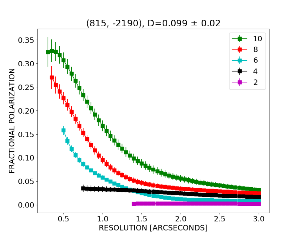
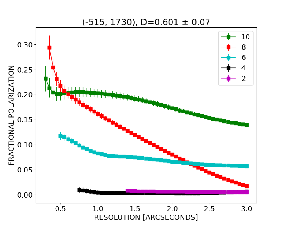
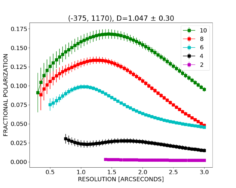
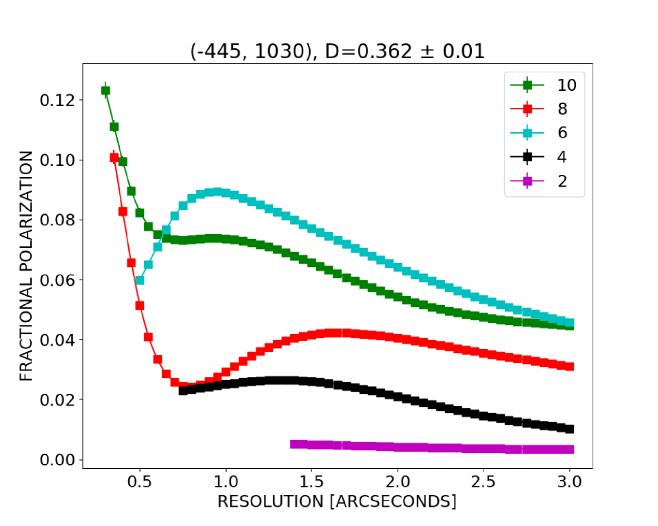
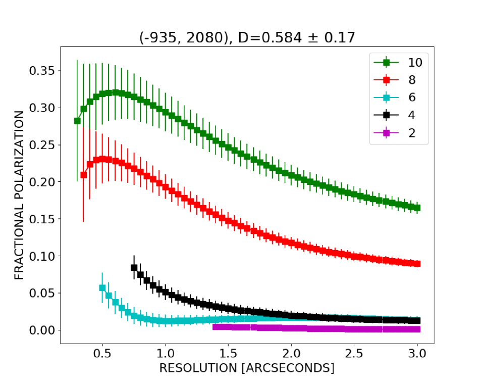
Figure 10: Lines-of-sight fractional polarization as a function of resolution. Green: 10 GHz. Red: 8 GHz. Cyan: 6 GHz. Black: 4 GHz. Magenta: 2 GHz. Plot titles: Lines-of-sight position coordinates and the RDR value at 3${}^{\prime\prime}/0.3^{\prime\prime}$ (10 GHz). Some lines-of-sight (top row) show the “expected” increase in fractional polarization with increasing resolution (these make up roughly 59% of the lines-of-sight). In some cases, we find lines-of-sight with fractional polarization changing unexpectedly with increasing resolution (two bottom rows, roughly 41% of the lines-of-sight behave this way).

5 Faraday Rotation

In the previous section, we demonstrated that Hydra A is experiencing both wavelength-dependent and resolution-related depolarization. These results imply the presence of a turbulent magneto-ionic medium on scales less than 1.5 kpc. At higher frequencies, we can achieve high resolution – which then minimizes beam-related effects. Moreover, the wavelength-dependent depolarization structures such as the sinc-like and complex decays are mostly concentrated at longer wavelengths. Thus, by utilizing the high frequency data, we can derive the ‘true’ emission properties of the source, without dealing with complicated depolarization structures.

We can then use these high-frequency, high-resolution approximations of the ‘true’ emission properties of the tails to predict the polarization characteristics at lower frequencies and lower resolution. A good match between such predictions with the observed data would provide strong evidence that a foreground, turbulent Faraday rotating medium is primarily responsible for the majority of the depolarization through beam-related effects.

We thus utilized the 6 - 12 GHz frequency data – which gives the highest resolution of $0.5\arcsec\times 0.35\arcsec$. By looking through the 553 lines-of-sight with suitable signal strength, we find that the structures in the depolarization functions are negligible within this frequency range. We thus fit to the fractional $Q$ and $U$ of our images the real and imaginary parts of the following model, respectively:

$$p=p_{0}e^{2i\chi_{0}}e^{2iRM\lambda^{2}-2\sigma_{t}^{2}\lambda^{4}},$$ (1)

where $p_{0}$ and $\chi_{0}$ are the zero-wavelength fractional polarization and polarization angle of the tails, respectively, $\mathrm{RM}$ is the rotation measure of the ambient medium with electron density $n_{e}$ [cm^-3], uniform magnetic field component, $\mathbf{B}_{u}$ [$\mu$G], located a distance $L$ [kpc] from us in $z$-axis direction:

$$RM=812\int\limits_{L}^{0}n_{e}\mathbf{B}_{u}\cdot\mathrm{dz}\quad\quad[\mathrm{rad\,m}^{-2}],$$ (2)

and where $\sigma_{t}$ quantifies the rate of depolarization with $\lambda^{2}$. It is commonly interpreted to be due to unresolved fluctuations in Faraday depths along lines of sight within the resolution beam. For a simple random turbulent screen, $\sigma_{t}$ is given by

$$\sigma_{t}=812n_{t}B_{t}d\sqrt{N}\quad\text{rad m${}^{-2}$},$$ (3)

and where $N=L/d$ is the number of turbulent cells of size $d$ along the total path length $L$, $n_{t}$ is the electron density in the cell, and $B_{t}$ is the magnetic field strength of the cell – representing a turbulent (assuming a random walk model) magnetic field strength (Burn, 1966; Sokoloff et al., 1998).

We use a simple non-linear least squares fitting algorithm for fitting this model to the data. This was done using minimization tools provided through the software package LMFIT. We wrote a specific code for this particular problem, which can be provided upon request. The fitting to fractional $Q$ and $U$ was performed simultaneously and the best-fitting parameters were those that minimize the difference in the data and model in both $Q$ and $U$.

We confined our search space between $0.0001$ and $1$ for $p_{0}$, $\pm\pi/2$ for $\chi_{0}$, $\pm 12500$ rad m^-2 for $\mathrm{RM}$ and [0, 2500] rad m^-2 for $\sigma$. We only considered pixels with flux density $>5\times$ the off-source noise of a 1 GHz Stokes $I$ image. This is so that we avoid evaluating spurious/noisy pixels, and also to reduce computational time. Figure 11 shows the example fits, indicating a reasonable fit of this model to the data.

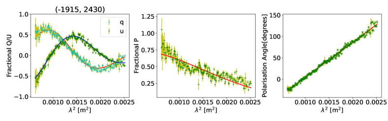
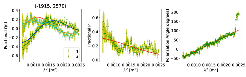
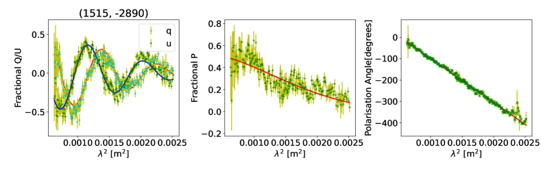
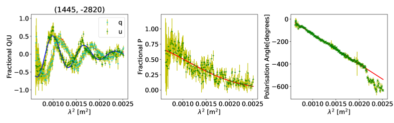
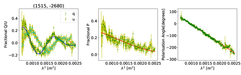
Figure 11: Example of fitting a simple random depolarization screen defined in Eq. 1 to the high resolution 6 - 12 GHz data. Left column shows fractional $Q$ and $U$, middle column shows fractional polarization, $p$, and right column show polarization angle all three as a function of $\lambda^{2}$.

Figure 12 shows maps of derived zero-wavelength (intrinsic) fractional polarization (top panel), rotation measures (middle panel), and dispersions (bottom panel). The left panel shows the northern tail, and right panel the southern tail. We display pixels with fitting error in $p_{0}$ less than 0.1.

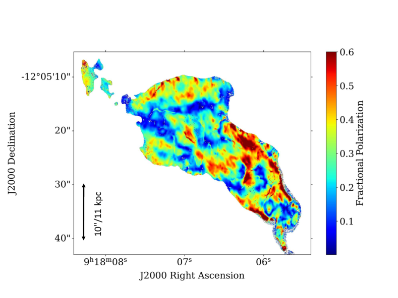
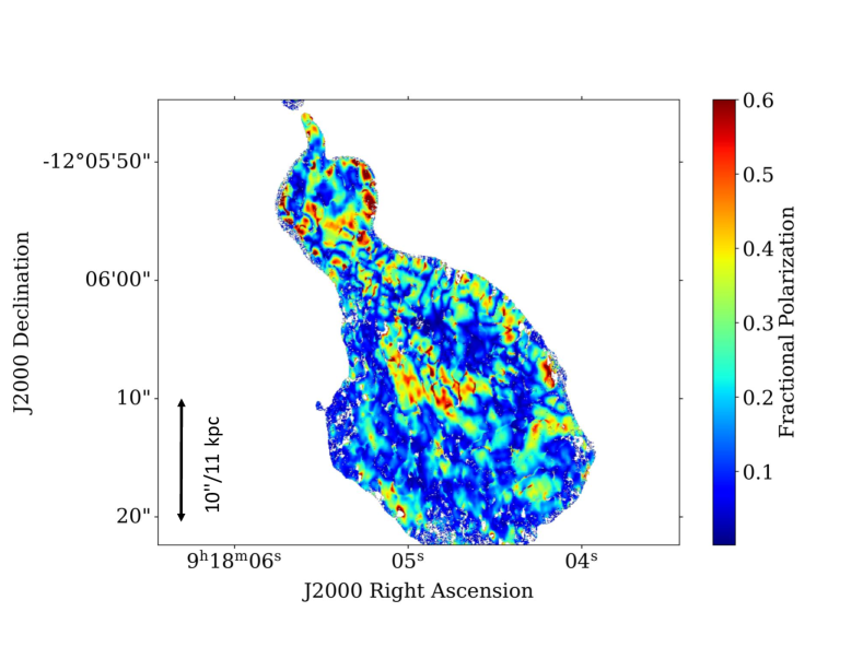
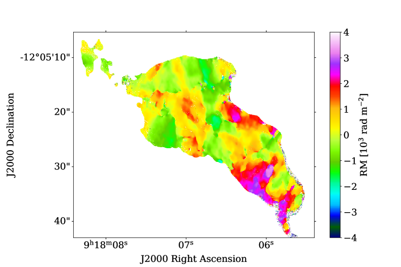
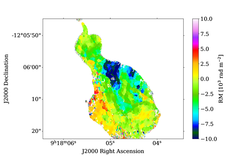
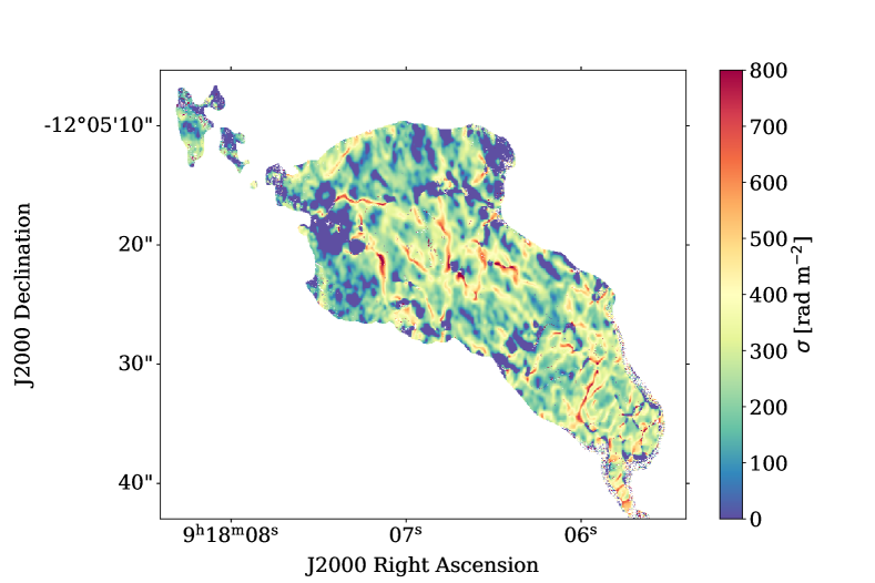
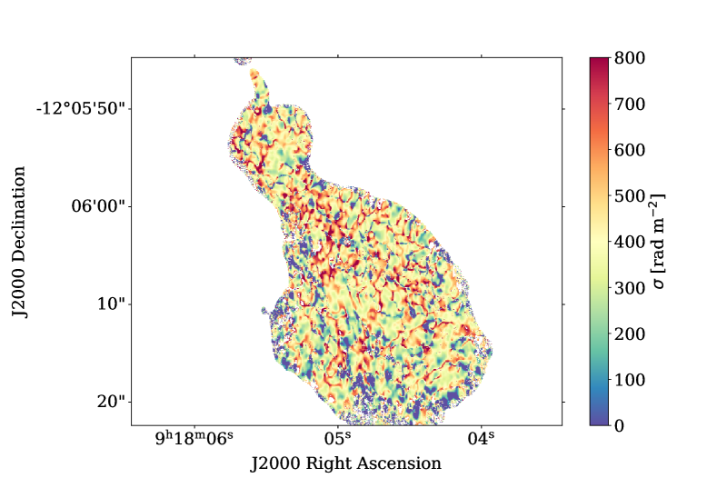
Figure 12: Parameters derived from fitting Eq. 1 to high frequency ($6-12$ GHz) high resolution $0.50\arcsec\times 0.35\arcsec$ polarization data. The left column shows the northern tail, and the right column shows the southern tail. The top row shows the intrinsic fractional polarization (extrapolated to zero $\lambda$), the middle row shows the rotation measure maps, and the third row is the $\mathrm{RM}$ dispersion. Shown are pixels with error in fractional polarization $<0.1$. The physical scale shown in the top panel is the true for the rest of the panels.

We discuss each of these derived images in the following sections.

5.1 Intrinsic Fractional Polarization

The derived zero-wavelength fractional polarizations indicate that Hydra A is intrinsically highly linearly polarized in both tails, with values ranging between 5% and 65% in the northern tail, and up to 75% at the edges of the tail. The southern tail is less polarized and extremely patchy – with polarization values as low as $2\%$, and as high as 55% in the inner regions of the tail, and up to 70% at the edges. The small-scale patchiness in the fractional polarization of this tail likely indicates that our resolution is still not sufficient to allow probing of the source properties, or that there is an interesting phenomenon occurring inside this tail, which is not present in the northern tail. We believe the former is probably what is taking place in this tail, especially since we have seen in Section 4 that the depolarization structures across this tail are mostly complex with rapid smooth-like decays which indicate the presence of small magnetic field scales. It should be noted that this does not rule out the possibility that this tail may be intrinsically different in its physical properties, but at this point there is no substantial evidence to support this claim.

5.2 Rotation Measures

The rotation measure maps presented here are much more detailed than those available in the literature (e.g., Taylor & Perley, 1993; Laing et al., 2008), due to the wide frequency span and continuous frequency sampling available in the new data. Rotation measures range between -2000 rad m^-2 and 3300 rad m^-2 across the northern tail, and -12300 rad m^-2 and 5000 rad m^-2 across the southern tail. They are mostly negative across the southern tail with a small region situated in the south-eastern parts of the tail with positive rotation measures. The rotation measures associated with this tail are remarkably patchy on scales of $\sim 1$ kpc. A region of extremely high rotation measures does not seem to be associated with any obvious tail features: neither in total intensity, fractional polarization, or dispersions – indicative of external (unrelated to the tail) origin. The rotation measures across the northern tail, on the other hand, are both negative and positive, and are relatively more ordered on scales of $\sim$ 2 to 6 kpc. They also seem to occur in alternating bands of positive and negative values. Alternating bands in $\mathrm{RM}$ have been observed in few cases in radio sources; they were observed in Cygnus A (Sebokolodi et al., 2020), as well as in M84, 3C 353, 0206+35, and 3C 270 (Guidetti et al., 2011). Similar to the results of Taylor & Perley (1993), the rotation measures across the jets are consistent with those of the nearby tail, suggesting a common origin.

Figure 13 shows histograms of $\mathrm{RM}$ distribution across the tails. The distributions are consistent with Figure 4 and 5 of Taylor & Perley (1993). We find a mean of 313 rad m^-2 and a standard deviation of 1298 rad m^-2 for the northern tail, a mean of -2049 rad m^-2 and a standard deviation of 3396 rad m^-2 across the southern tail. The mean $\mathrm{RM}$ across the northern tail is significantly different from that of Taylor & Perley (1993)), but the standard deviation is similar. For the southern tail, the mean and standard deviation are different from those of Taylor & Perley (1993). This difference is likely due to the difference in the $\mathrm{RM}$ range, with our distribution showing $\mathrm{RM}$s above 2000 rad m^-2. Our data show bumps in $\mathrm{RM}$ at 2000 rad m^-2 in the northern tail and -8000 rad m^-2 in the southern tail. The latter was also seen by Taylor & Perley (1993). The bump in the northern tail is slightly visible in Taylor & Perley (1993). The mean and spread in $\mathrm{RM}$ distribution of the two tails is extremely different, suggesting the astrophysical situation is remarkably different for the two tails, either within the tails or in their local environment, on scales of $\sim$30 kpc (the extent of the individual tail).

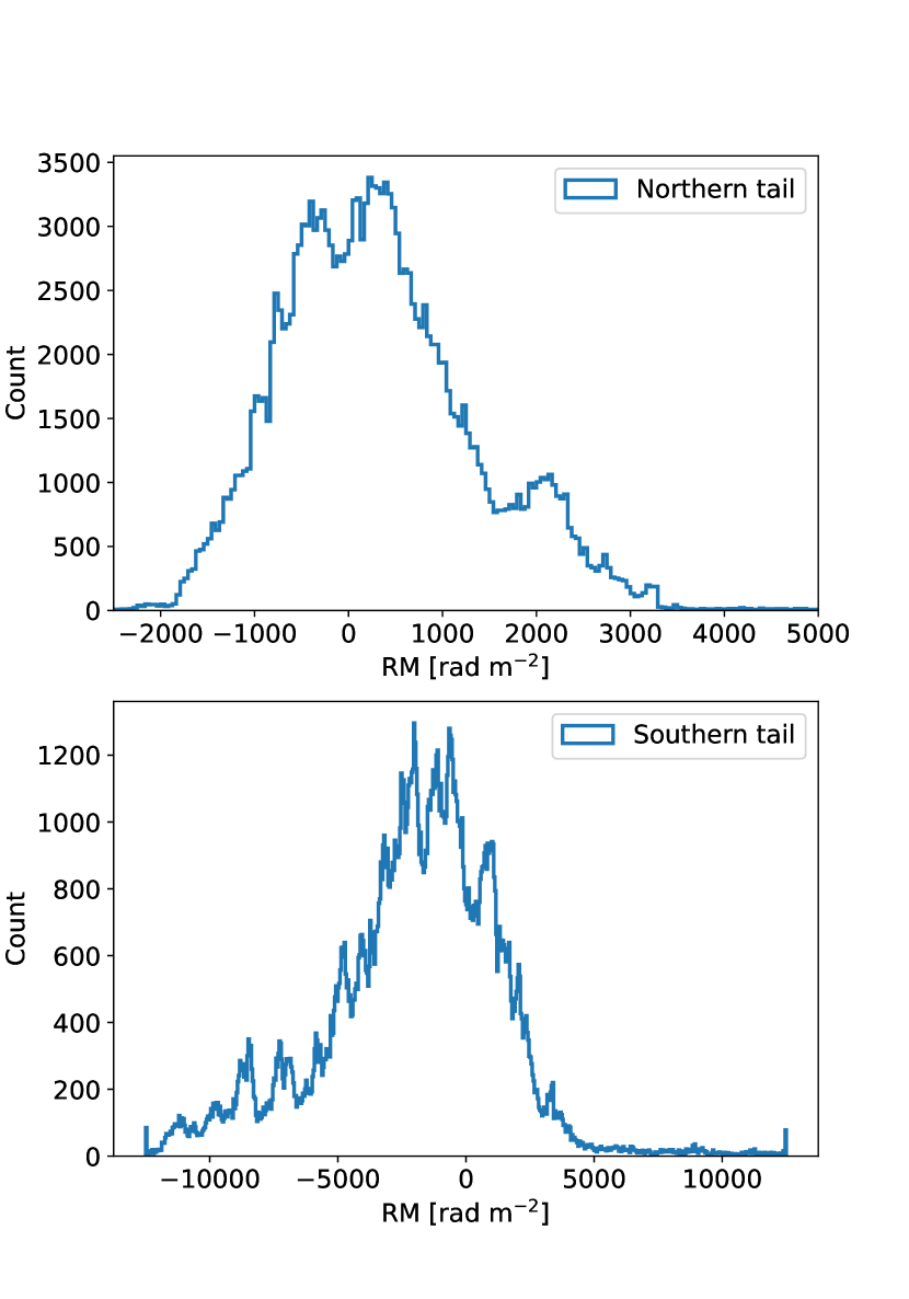
Figure 13: A histogram of RM distribution across both tails (in bins of 600). We find a mean of 313 rad m^-2 and a standard deviation of 1298 rad m^-2 for the northern tail, and a mean of -2049 rad m^-2 and a standard deviation of 3396 rad m^-2 across the southern tail.

Figure 14 shows the $\mathrm{RM}$ profile of the tails along the declination. The profile was obtained by computing the statistics of $\mathrm{RM}$s across all right ascension for a specific declination. The estimates were made across bins of 50 pixels (2.5^′′). In red, we show the mean (data points) and standard deviation (shade), and in blue is the median (data points) and first and third quartile in shade. The magnitude of $\mathrm{RM}$s across the northern tail reduces radially outward, showing non-uniform oscillations. The magnitudes of the $\mathrm{RM}$s across the southern tail increase radially outward until reaching a maximum at (RA, Dec) = $(10^{\prime\prime},20^{\prime\prime})$, and then decrease beyond 20^′′ to $\sim 0$ rad m^-2, and begins to increase and change sign. The $\mathrm{RM}$ changes smoothly – there are no large jumps between successive regions (with the exception of the high $\mathrm{RM}$ region in the southern tail). Notably, the $\mathrm{RM}$ smoothly reduces close to $0$ rad m^-2 before changing sign. This profile is consistent with the profile obtained by Taylor & Perley (1993) (see Figure 7).

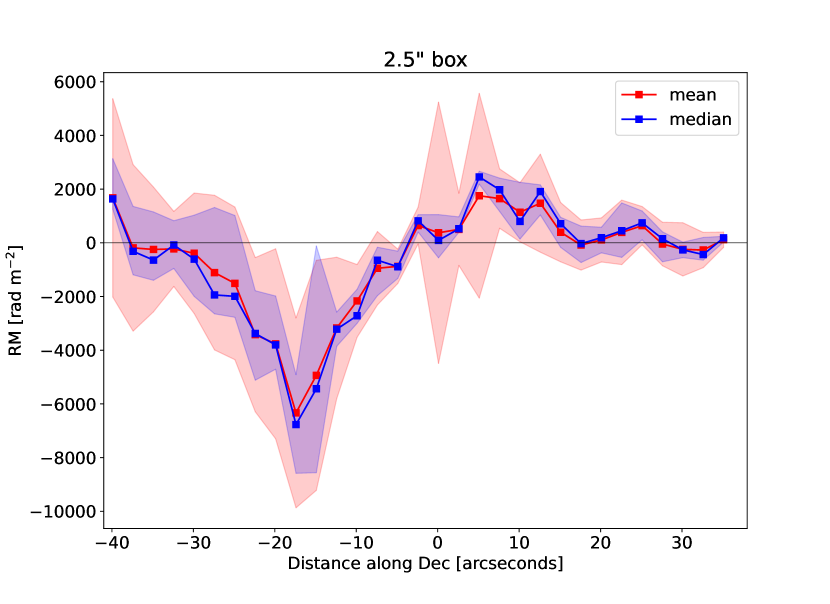
Figure 14: The $\mathrm{RM}$ profile as a function of distance from the image center along declination, in bins of 50 pixels (2.5^′′). The mean of $\mathrm{RM}$s computed across RA is shown in red data points and a standard deviation in a red shade. The median is shown in blue data points, the first and third quartile in blue shade. The $\mathrm{RM}$ profile is consistent with that of Taylor & Perley (1993).

5.3 Faraday Dispersions

This metric characterizes the rate of depolarization between 12 GHz and 6 GHz, at a resolution of $0.5\arcsec\times 0.35\arcsec$. Figure 15 shows the distribution of the $\mathrm{RM}$ dispersions more clearly. The dispersions in the northern tail range roughly between 0 and 800 rad m^-2, with most regions of the tail $<450$ rad m^-2. The dispersions across the southern tail range between 0 and 1000 rad m^-2, with the majority concentrated $\lesssim$ 800 rad m^-2. The large dispersions are associated with narrow regions. These narrow regions are relatively common across the southern tail. The majority of the dispersions are associated with fitting errors $\lesssim$ 100 rad m^-2. The dispersions $\leq$ 20 rad m^-2 and $\geq$ 1500 rad m^-2 are associated with very large errors, and are therefore, not reliable (most of which are failed fits). The large dispersions are removed after applying the masking approach noted in Fig 15 caption, which masks pixels with fractional error in $p_{0}<0.1$.

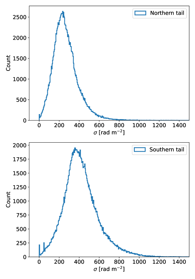
Figure 15: A histogram of $\mathrm{RM}$ dispersions distribution across both tails (in bins of 600). We find a mean of 234 rad m^-2 and a standard deviation of 200 rad m^-2 for the northern tail and a mean of 380 rad m^-2 and a standard deviation of 226 rad m^-2 across the southern tail. The $\sigma$ range roughly between 0 rad m^-2 and 800 rad m^-2 for the northern tail, and 0 rad m^-2 and 1000 rad m^-2 for the southern tail.

Figure 16 shows the $\sigma_{t}$ profiles along declination. The dispersions across the southern tail decrease steadily with radius, while the dispersions decrease rapidly with radius across the northern tail. There is no correlation between $\mathrm{RM}$ and $\sigma_{t}$ profile in the southern tail (see Figures 14 and 16), while both quantities decrease radially in the northern tail.

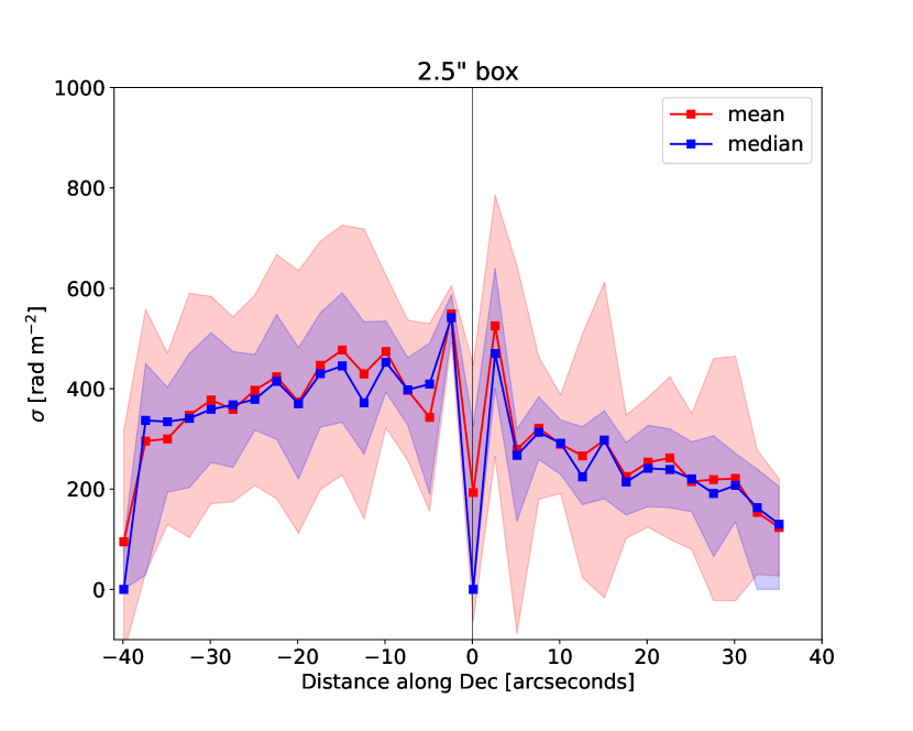
Figure 16: $\mathrm{RM}$ dispersion profile as a function of distance from the image center along declination, in bins of 50 pixels (2.5^′′). The mean of dispersions computed across RA is shown in red data points and standard deviation in a red shade. The median is shown in blue data points, the first and third quartile in a blue shade.

5.4 Intrinsic Projected Magnetic Field Orientation

Figure 17 shows the intrinsic magnetic field orientation across the tails obtained by adding $\pi/2$ to the derived intrinsic polarization angle, $\chi_{0}$. The fields follow the boundaries and filamentary structures of the tail emission. This behavior is quite common in radio galaxies, for example 3C 465 (Eilek, & Owen, 2002), Cygnus A (Dreher et al., 1987; Sebokolodi et al., 2020), and Pictor A (Perley et al., 1997), and is generally understood as an effect resulting from shearing (and compression at outer parts of the tails) of the tangled magnetic field at the tail boundary, resulting in suppression of field components normal to the tail boundaries (Laing, 1980). The field vectors are generally smooth across the northern tail, while slightly chaotic across the southern tail. As with the other fitted parameters, this is likely due to significant structures on scales less than the $0.5\arcsec$ resolution utilized here.

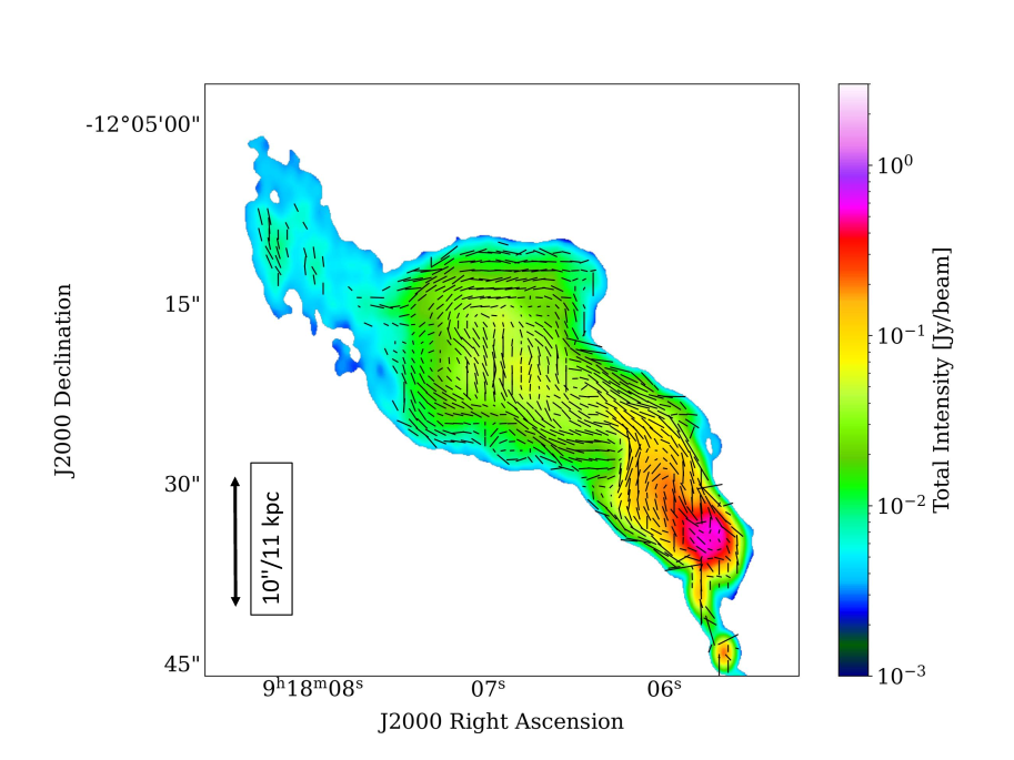
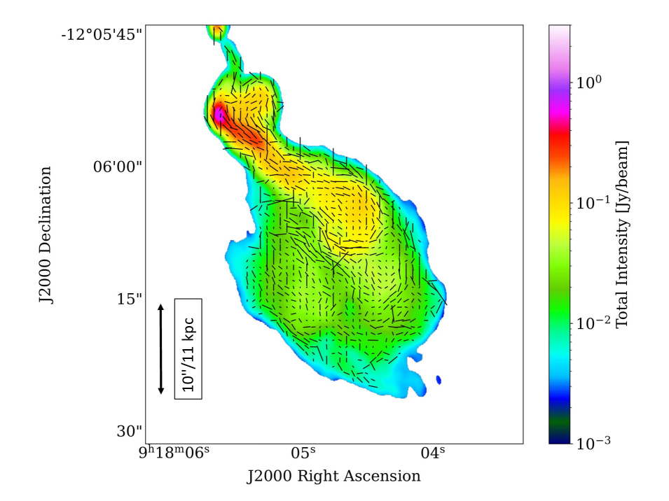
Figure 17: Magnetic field orientations superimposed on a 2 GHz total intensity map. The vector lengths are proportional to the fractional polarization (magnified by a factor of 30). Showing only pixels with fitting error in $p_{0}<0.1$.

5.5 A Curious V-shaped Structure in Northern Tail

An examination of the highest resolution intensity image from the inner part of the northern tail shows a distinct ‘V’-shaped feature. It sits $\sim 12$ kpc north of the galactic core and is oriented roughly along the local direction of the tail. It is apparent in total intensity and is also traced by projected magnetic field lines. However, there is only a small effect in the fractional polarization on the ‘V’-shape. A close-up image is shown in Figure 18. The apex of the ‘V’ points toward the galaxy, which is also the presumed ‘upstream’ direction relative to the systematic outflow likely to be moving through the northern bright spot.

We do not know the cause of this structure, however, its shape suggests a bow shock or magnetic draping around an object within the tail. If it is a bow shock, its opening angle requires a Mach number of $\sim 3-4$. Although large-scale tails in FR I sources are thought to be subsonic, the jets close to the AGN are likely supersonic. If this is the case in Hydra A, the supersonic flow may continue through the growth of the instability which causes the bright spot and changes the narrow inner jet to a broad tail. Alternatively, a slower flow can “drape” a weak magnetic field around an object in the flow (for example, Lyutikov, 2006; Dursi & Pfrommer, 2008) and can also explain the ordered magnetic fields along the sides of the structure. A third possibility suggested by the ‘V’-shape could be a wake behind some object in the flow. However, the ordered magnetic field along the sides of the ‘V’ seems inconsistent with the turbulence characteristic of subsonic wakes.

Each of these possibilities depends on the existence of a dense object – say a cold gas cloud – within the flow. The inner regions of many galaxies in cool-core clusters contain filaments and clouds of thermal and molecular gas (Olivares et al., 2019). Similar objects might exist in the Hydra A galaxy, however they have not yet been detected. The Hydra A galaxy contains a $5$ kpc cool gas disk, rotating around the core of the central galaxy (Rose et al., 2019) but no $H\alpha$ or molecular emission has been detected yet outside of this disk.

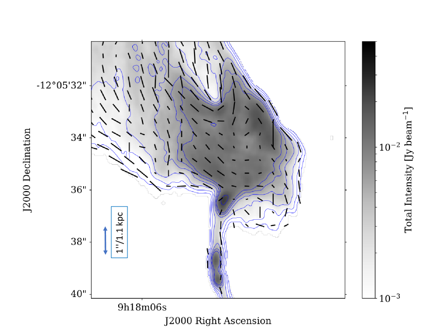
Figure 18: The ‘V’-shaped structure in brightness and magnetic fields in the northern tail of Hydra A. The orientation vectors correspond to the magnetic field orientation and the lengths are proportional to the fractional polarization. The magnetic field orientation traces the ‘V’, while the fractional polarization has a minimal effect.

6 Predictions of Low-Frequency Data

In section 4.2 we showed that interpretation of the Hydra A depolarization data is limited by resolution – our observations do not provide enough resolution to properly resolve out the variations occurring across the tail. Although it is clear that the beam-related effects are important, can we really claim that they are the dominant effects responsible for the majority of the depolarization? This question can only be fully answered with high resolution observations, particularly at low frequencies. Based on our current data, we would need resolutions much better than 0.30$\arcsec$ (perhaps 10 times better), at frequencies down to 2 GHz, to determine the significance of the beam depolarization to the overall depolarization. Instruments with such observing capability are currently not available. We have thus developed a method of using the high-frequency, high-resolution images of the $\mathrm{RM}$ and polarized emission to predict the lower resolution, lower frequency emission properties. Comparison of the observed with the predicted emission will then allow a judgement on whether the assumptions inherent in the prediction are correct. The basic assumption here is that these high-resolution maps approximate that of the true emission of the tails and rotating gas. A close prediction will be a strong indication for a foreground turbulent Faraday rotating screen. A mis-match will indicate either the presence of much smaller scales ($\ll 0.3\arcsec$), which we could not accurately model, or that the beam-related effects are not a dominant effect, and the depolarization is due to a different physical origin. Both of these have an important physical implication, but this is out of scope for this paper.

Given the derived $p_{0}$, $\chi_{0}$, and $\mathrm{RM}$, from the high-resolution, high-frequency images, we calculate the model polarized flux as

$$P=p_{0}Ie^{2i\chi_{0}}e^{2iRM\lambda^{2}}.$$ (4)

We obtain $I$ by first determining the spectral index at $0.50\arcsec\times 0.35\arcsec$ (using 6 -12 GHz data), and using this spectral index map to predict total intensities across 2 - 12 GHz. The polarized emission in Eq. 4 is computed for $\lambda^{2}$ between 2 - 12 GHz – the resulting polarized cube has a resolution of the input maps; $0.50\arcsec\times 0.35\arcsec$. We then obtain Stokes $Q$ and $U$ by taking the real and imaginary part of Eq. 4, then convolve these Stokes maps, including Stokes $I$ to $1.50\arcsec\times 1.0\arcsec$. The convolution is done using AIPS task CONVL, with factor input as $0$. This is the same procedure applied in the case of Cygnus A (Sebokolodi et al., 2020). Our simple modelling does not take into consideration the observing noise.

Figure 19 shows the predictions in red, and the actual data in black. The plots show fractional polarization as a function of $\lambda^{2}$ in the left panel, polarization as a function of $\lambda^{2}$ in the middle column, and Faraday spectra in the right panel. We compared the data and the predicted data based on fractional polarization (left panel). The top two rows show examples of the lines-of-sight whose data are predicted well to within measurement errors – with roughly 4.1% of the lines-of-sight reproduced reasonably well. We find that these lines-of-sight are not in any way special: they neither occupy a special spatial location, nor do they occupy a special region in the parameter spaces (e.g. Stokes $I$, fitted $p_{0}$, $\mathrm{RM}$ and $\sigma_{t}$). The remaining rows show those whose general depolarization pattern/structure is being reproduced but with slight differences due to either the underestimation of the depolarization, and/or the shift in the nulls of the oscillations. We find that roughly 70.5% of the lines-of-sight are partially reproduced. The remaining 25.4 % are poorly predicted, or are too noisy to make any accurate judgment.

Although this approach is simple and naive, we find that the depolarization structures that are seen in the data are, overall, reproduced remarkably well. This has an important implication – that the structures in the rotation measure map are responsible for the observed depolarization. This suggests that beam-related effects are the main contributor to the observed depolarization. The misalignment of the nulls in the sinc-like lines-of-sight occur very rarely, while the underestimation of the depolarization is common. These underestimations may be a result of unmodelled small-scale fluctuations and/or systematic errors in the prediction model. Thus, we emphasize that these predictions should be treated as indicative, not as a complete proof.

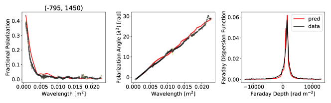
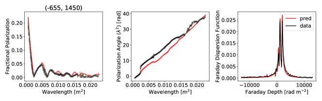
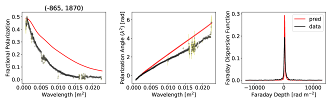
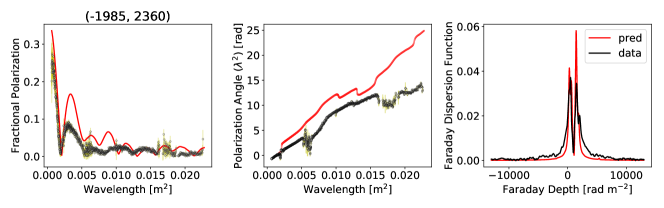
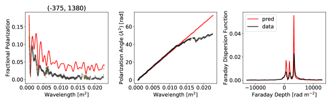
Figure 19: Predictions of low-frequency, low-resolution depolarization using high-resolution polarization and $\mathrm{RM}$ maps derived from high-resolution, high-frequency data. Left column: Fractional polarization vs $\lambda^{2}$. Middle column: Polarization angle vs $\lambda^{2}$. Right column: Faraday spectra. Black: Observed data. Red: Predictions. Two top rows: Reasonably good predictions (roughly $4\%$ of the lines-of-sight). Last three rows: Partially reproduced ($71\%$).

7 Summary

In this paper we have presented initial results from our wideband (2 - 12 GHz), high spectral resolution polarimetry data on Hydra A. We look at how the source polarization emission changes across both frequency and resolution. We have also derived high resolution maps of the intrinsic polarized emission of the tails ($p_{0}e^{2i\chi_{0}}$), the rotation measure ($\mathrm{RM}$) and Faraday dispersion ($\sigma_{t}$) of a foreground cluster gas. Further, we used these high resolution maps to predict the data at low frequencies and low resolution.

The results are summarized as follows:

1. The tails including the jets depolarize globally with decreasing frequency, with regions closest to the nucleus depolarizing more quickly than those far away.

2. The fractional polarization across the northern tail is smooth at high frequencies while the southern tail is relatively patchier. However, both tails become clumpy at lower frequencies.

3. We find that the tails depolarize by more than 90% between 10 GHz and 2 GHz.

4. Fractional polarization as a function of $\lambda^{2}$ of the different lines-of-sight across the tails reveals very complex depolarization behavior, with some lines-of-sight showing smooth decaying fractional polarization, some are sinc-like and others are complex/intermediate. The depolarization across the southern tail is mostly complex, with a few smooth decays. The northern tail consist of the three depolarization structure with the smooth decay concentrated at extreme regions of the tail (further from the nucleus).

5. We derived Faraday spectra of the lines-of-sight using RM-Synthesis, and we find interesting structures in the spectra. In general the spectra for smooth decaying lines-of-sight consist of single (or few closely-separated) peak(s), while the spectra of sinc-like and complex decays are complicated, showing multiple peaks, and large broadening.

6. Polarization angle as function of $\lambda^{2}$ show significant deviations from linearity ($>1$ rad). Most deviations are associated with multiple-peaked Faraday spectra.

7. We find that the tails depolarize with decreasing resolution, with the inner regions depolarizing more rapidly than regions further from the nucleus.

8. The fractional polarization across the tail decreases with decreasing resolution for most lines-of-sight. However, for some lines-of-sight the fractional polarization changes in an unpredictable manner by decreasing at high resolution and changing abruptly across resolution – indicating very complex beam-related effects.

9. The rotation measures, $\mathrm{RM}$, across the northern tail range between $2000$ rad m^-2 and 3300 rad m^-2, and between $-2000$ rad m^-2 and $\sim$ 11900 rad m^-2 across the southern tail. The rotation measures occur on scales of 2 to 6 kpc in the northern tail, and very small scales of $\sim$ 1 kpc across the southern tail. Rotation measures across the northern tail show bands of alternating positive and negative values. Those of the southern tail are mostly negative, with a small region of positive values situated in the outskirts of the tail (south-east).

10. The derived intrinsic fractional polarization at 0.5″$\times$0.35″shows polarization of 20% to 50% across the northern tail, and 0.5% to 50% across the southern tail. There are also highly polarized region of up to 65% at the edge of the northern tail (west side), and narrow regions of up to 70% polarization across the southern tail. In general, the southern tail is relatively less polarized, and patchy. The southern tail may be intrinsically different or it could be that we haven’t fully resolved structures across the tail. We argue that the latter is probably the major reason for the observed polarization behavior, but our data cannot disprove any intrinsic phenomena.

11. The magnetic field orientation of the source follows the boundary and filamentary structures of the tails – consistent with other radio galaxies. The orientations are slightly chaotic in the southern tail.

12. The rotation measure dispersions range between 150 rad m^-2 and 350 rad m^-2 across the northern tail, and 300 rad m^-2 and 950 rad m^-2. The dispersions show no radial dependence. The dispersions are extremely chaotic across the southern tail – with narrow regions of high dispersions. These are associated with large gradients.

13. We used the derived intrinsic fractional polarization, and rotation measures at high resolutions (0.5″$\times$0.35″) to predict low frequency, low resolution data (1.50″$\times$1.0″). The assumption is that these high resolution maps present a close representation of the ’true’ source properties and foreground Faraday rotating medium. We find that the depolarization structure in the data are reproduced – with a few 4.1% closely reproduced, and 70.5% partially reproduced. For the latter, the depolarizations are mostly underestimated, and in some rare cases the nulls in the sinc-like decay are shifted to low frequencies. These results suggest that the depolarization is mostly a result of small-scale fluctuations across a foreground Faraday rotating medium. This depolarizing medium must consist of multiscale magnetic fields ordered on scales 0.30 - 1.5 kpc.

8 acknowledgments

The financial assistance of the South African Radio Astronomy Observatory (SARAO) towards this research is hereby acknowledged (www.ska.ac.za). Additional financial assistance was provided by the National Radio Astronomy Observatory – a facility of the National Science Foundation operated under cooperative agreement by Associated Universities, Inc. This work is based upon research supported by the South African Research Chairs Initiative of the Department of Science and Technology and National Research Foundation.

References

- Abell (1958) Abell, G. O. 1958, ApJS, 3, 211
- Anderson et al. (2016) Anderson, C. S., Gaensler, B. M., & Feain, I. J. 2016, ApJ, 825, 59.
- Baum et al. (1988) Baum, S. A., Heckman, T. M., Bridle, A., et al. 1988, ApJS, 68, 643
- Blanton et al. (2001) Blanton, E. L., Sarazin, C. L., McNamara, B. R., et al. 2001, ApJ, 558, L15
- Boehringer et al. (1993) Boehringer, H., Voges, W., Fabian, A. C., et al. 1993, MNRAS, 264, L25
- Burn (1966) Burn, B. J. 1966, MNRAS, 133, 67
- Brentjens & de Bruyn (2005) Brentjens, M. A., & de Bruyn, A. G. 2005, A&A, 441, 1217
- Carilli et al. (1994) Carilli, C. L., Perley, R. A., & Harris, D. E. 1994, MNRAS, 270, 173
- Cotton et al. (2009) Cotton, W. D., Mason, B. S., Dicker, S. R., et al. 2009, ApJ, 701, 1872.
- David et al. (1990) David, L. P., Arnaud, K. A., Forman, W., et al. 1990, ApJ, 356, 32
- David et al. (2001) David, L. P., Nulsen, P. E. J., McNamara, B. R., et al. 2001, ApJ, 557, 546
- Dreher et al. (1987) Dreher, J. W., Carilli, C. L., & Perley, R. A. 1987, ApJ, 316, 611
- Dwarakanath et al. (1995) Dwarakanath, K. S., Owen, F. N., & van Gorkom, J. H. 1995, ApJ, 442, L1
- Dursi & Pfrommer (2008) Dursi, L. J. & Pfrommer, C. 2008, ApJ, 677, 993.
- Eilek, & Owen (2002) Eilek, J. A., & Owen, F. N. 2002, ApJ, 567, 202
- Fabian et al. (2000) Fabian, A. C., Sanders, J. S., Ettori, S., et al. 2000, MNRAS, 318, L65
- Fabian et al. (2003) Fabian, A. C., Sanders, J. S., Allen, S. W., et al. 2003, MNRAS, 344, L43
- Garrington et al. (1991) Garrington, S. T., Conway, R. G., & Leahy, J. P. 1991, MNRAS, 250, 171
- Guidetti et al. (2011) Guidetti, D., Laing, R. A., Bridle, A. H., et al. 2011, MNRAS, 413, 2525
- Greisen (1990) Greisen, E. W. 1990, Acquisition, Processing and Archiving of Astronomical Images, 125
- Heinz et al. (2002) Heinz, S., Choi, Y.-Y., Reynolds, C. S., et al. 2002, ApJ, 569, L79
- Hutschenreuter et al. (2022) Hutschenreuter, S., Anderson, C. S., Betti, S., et al. 2022, A&A, 657, A43
- Kuchar & Enßlin (2011) Kuchar, P. & Enßlin, T. A. 2011, A&A, 529, A13.
- Laing (1980) Laing, R. A. 1980, MNRAS, 193, 439
- Laing (1988) Laing, R. A. 1988, Nature, 331, 149
- Laing et al. (2008) Laing, R. A., Bridle, A. H., Parma, P., et al. 2008, MNRAS, 391, 521
- Lane et al. (2004) Lane, W. M., Clarke, T. E., Taylor, G. B., et al. 2004, AJ, 127, 48
- Lyutikov (2006) Lyutikov, M. 2006, MNRAS, 373, 73.
- McNamara et al. (2000) McNamara, B. R., Wise, M., Nulsen, P. E. J., et al. 2000, ApJ, 534, L135
- Ma et al. (2019) Ma, Y. K., Mao, S. A., Stil, J., et al. 2019, MNRAS, 487, 3432.
- Nulsen et al. (2002) Nulsen, P. E. J., David, L. P., McNamara, B. R., et al. 2002, ApJ, 568, 163
- Nulsen et al. (2005) Nulsen, P. E. J., McNamara, B. R., Wise, M. W., et al. 2005, ApJ, 628, 629
- Owen et al. (1995) Owen, F. N., Ledlow, M. J., & Keel, W. C. 1995, AJ, 109, 14
- Olivares et al. (2019) Olivares, V., Salome, P., Combes, F., et al. 2019, A&A, 631, A22.
- O’Sullivan et al. (2012) O’Sullivan, S. P., Brown, S., Robishaw, T., et al. 2012, MNRAS, 421, 3300.
- Perley et al. (1997) Perley, R. A., Roser, H.-J., & Meisenheimer, K. 1997, A&A, 328, 12
- Perley et al. (2001) Perley, R.A., Chandler, C.J., Butler, B.J., and Wrobel, J.M. 2001 ApJ, Lett, 739:L1
- Rose et al. (2019) Rose, T., Edge, A. C., Combes, F., et al. 2019, MNRAS, 485, 229.
- Riseley et al. (2020) Riseley, C. J., Galvin, T. J., Sobey, C., et al. 2020, PASA, 37, e029.
- Sebokolodi et al. (2020) Sebokolodi, M. L., Perley, R., Eilek, J., et al. 2020, ApJ, 903, 36
- Simionescu et al. (2009) Simionescu, A., Roediger, E., Nulsen, P. E. J., et al. 2009, A&A, 495, 721
- Snios et al. (2018) Snios, B., Nulsen, P. E. J., Wise, M. W., et al. 2018, ApJ, 855, 71
- Sokoloff et al. (1998) Sokoloff, D. D., Bykov, A. A., Shukurov, A., et al. 1998, MNRAS, 299, 189
- Stuardi et al. (2020) Stuardi, C., O’Sullivan, S. P., Bonafede, A., et al. 2020, A&A, 638, A48.
- Taylor et al. (1990) Taylor, G. B., Perley, R. A., Inoue, M., et al. 1990, ApJ, 360, 41
- Taylor & Perley (1993) Taylor, G. B., & Perley, R. A. 1993, ApJ, 416, 554
- Taylor (1996) Taylor, G. B. 1996, ApJ, 470, 394
- van Moorsel et al. (1996) van Moorsel, G., Kemball, A., & Greisen, E. 1996, Astronomical Data Analysis Software and Systems V, 37
- Vogt & Enßlin (2005) Vogt, C. & Enßlin, T. A. 2005, A&A, 434, 67.
- Young et al. (2002) Young, A. J., Wilson, A. S., & Mundell, C. G. 2002, ApJ, 579, 560