Phase field modeling of brittle compressive-shear fractures in rock-like materials: a new driving force and a hybrid formulation

Abstract

Compressive-shear fracture is commonly observed in rock-like materials. However, this fracture type cannot be captured by current phase field models (PFMs), which have been proven an effective tool for modeling fracture initiation, propagation, coalescence, and branching in solids. The existing PFMs also cannot describe the influence of cohesion and internal friction angle on load-displacement curve during compression tests. Therefore, to develop a new phase field model that can simulate well compressive-shear fractures in rock-like materials, we construct a new driving force in the evolution equation of phase field. Strain spectral decomposition is applied and only the compressive part of the strain is used in the new driving force with consideration of the influence of cohesion and internal friction angle. For ease of implementation, a hybrid formulation is established for the phase field modeling. Then, we test the brittle compressive-shear fractures in uniaxial compression tests on intact rock-like specimens as well as those with a single or two parallel inclined flaws. All numerical results are in good agreement with the experimental observation, validating the feasibility and practicability of the proposed PFM for simulating brittle compressive-shear fractures.

1 Department of Geotechnical Engineering, College of Civil Engineering, Tongji University, Shanghai 200092, P.R. China
2 Institute of Continuum Mechanics, Leibniz University Hannover, Hannover 30167, Germany
3 Division of Computational Mechanics, Ton Duc Thang University, Ho Chi Minh City, Viet Nam
4 Faculty of Civil Engineering, Ton Duc Thang University, Ho Chi Minh City, Viet Nam
* Corresponding author: Xiaoying Zhuang (zhuang@ikm.uni-hannover.de)

Keywords: Phase field model, Rock-like material, Compressive-shear fracture, Driving force, Hybrid formulation, Strain decomposition

1 Introduction

Geomaterial failure dominated by shear or compressive fractures is commonly observed in underground engineering. However, the prediction of fractures in rock-like solids remains a challenging topic especially for complex fracture patterns. One major reason of this is that geological media generally have many intrinsic flaws such as micro cracks, voids and soft minerals [1; 2; 3], which drastically increase the complexity of fracture propagation in the geomaterials. One direct way to explore the fracture mechanisms is to establish experimental tests and there have been many studies carried out regarding the fracture propagation in rock-like materials; see for instance the contributions in Lajtai [4]; Sagong and Bobet [5]; Wong and Einstein [6]; Yang and Jing [7]; Basu et al. [8]; Xia et al. [9]; Zhou et al. [10, 11]. Although experimental tests can observe basic phenomenon and provide guidance for empirical studies, they are generally limited by the loading conditions and observations of the fracture pattern evolution. Furthermore, many physical quantities cannot be measured directly, e.g. stress/strain near crack tips. Therefore, numerical approaches have become important and complementary alternative and are attracting increasing interests because they can help to understand the mechanism and are less expensive than experimental tests.

In the past decade, a variety of numerical methods have been developed for capturing fracture phenomena and providing distinctive physical insights that cannot be obtained through experimental tests alone [3]. These numerical methods can be categorized into two categories, namely the discrete approach and smeared approach according to the different treatments of strong discontinuities in the displacement field across the fracture interfaces. For the discrete approaches, a sharp fracture model is introduced in modeling either explicitly [12] or implicitly [13; 14]. Among these methods, the extended finite element method (XFEM) [13; 14; 15; 16; 17], generalized finite element method (GFEM) [18], and the phantom-node method [19; 20] have been extensively applied and developed in recent years. In contrast to the discrete approaches, the smeared approaches diffuse the fracture by using smooth transitions between the intact material and fully damaged material [21]; therefore the displacement field is in a sense still continuous. Popular smeared approaches include gradient damage models [22], screened-Poisson models [23; 24] and phase field methods (PFMs) [25; 26; 27].

Among those smeared methods, PFMs have shown great potentials for complex fracture failure especially for multi-field problem [28; 27; 29; 30; 31; 3; 32; 33]. The origin of PFMs for brittle fractures can be traced back to Bourdin et al. [28] and later on the first thermodynamic consistent formulation of PFM was not proposed until Miehe et al. [26]. The original PFM and its successors all introduce an additional scalar field (the so-called phase field) to represent the evolution of fracture. Therefore, the sharp fracture is represented by a diffusive ’damage-like’ zone with the zone width is controlled by a length scale parameter. By using the variational approach the phase field modeling of fractures becomes a multi-field problem, namely phase field and mechanical field, and fracture propagation is easily obtained by solving partial differential equations. This results in a natural detection and tracking of fracture paths without any additional crack growth criteria [27], and for this reason PFM is believed to be a promising way to model complex fracture growth such as fracture arrest, deflection, branching, percolation and coalescence.

To date, PFMs have been extensively used to simulate a wide variety of fracture problems including dynamic fracture [27; 34; 30], ductile fracture [35; 36; 37; 38], cohesive fracture [39; 40; 34], fractures in thin shells and plates [36], fractures in functionally graded materials and composites [41; 42], and fluid-driven fractures [43; 44; 45; 46; 47; 48], while some implementations in FEM software such as COMSOL [30] and FEniCS [49] accelerate the application of PFMs. However, the applications and improvements of the PFM for fractures in rock-like materials are relatively limited and far from practical application. For example, only mode I tensile dominated fractures can be simulated such as the Brazilian tests [33; 50; 32], notched semi-circular bend (NSCB) tests [3], direct tension tests [3], and the hydraulic fractures [31; 45]. Furthermore, in the geological environment, geomaterials are often subjected to compressive principal stresses and compressive-shear fractures are commonly observed. This means that shear fractures will initiate and propagate even when all principal strains of the material are compressive. In contrast to this fact, the compressive-shear fractures cannot be predicted by the current PFMs for rock-like solids [21; 51; 52], where the negative strains and the compressive part of elastic energy are assumed not to contribute to the evolution of phase field. More specifically, the first attempt of the PFM for mixed-mode crack propagation in rock-like materials was proposed by Zhang et al. [21]. This method was established by introducing the critical energy release rate of mode II and two historic energy references in the model of Miehe et al. [26]. Choo and Sun [51] coupled a pressure-sensitive plasticity model with a phase field approach to capture brittle fracture, ductile flow, and their transition in rocks. Bryant and Sun [52] proposed a kinematic-consistent phase field approach to model mixed-mode fractures in anisotropic rocks. On the other hand, the contributions in Zhang et al. [21]; Choo and Sun [51]; Bryant and Sun [52] also show that the PFMs developed so far do not account for the influence of cohesion and internal friction angle on fracture propagation and the load-displacement curve. This is a missing aspect since it is generally accepted that a rock-like material will have a higher compressive strength if its cohesion or internal friction angle increases. Therefore, it is an imperative task to further develop PFM in order to be able to better predict the phenomena in rock failure.

In this study, we propose a new phase field model for simulating brittle compressive-shear fractures in rock-like materials by introducing a new driving force term, called $H_{p}$ in the evolution equation of the phase field. By using the spectral decomposition, this new driving force is established using the negative parts of the strain. In addition, the influence of cohesion and internal friction angle is considered in the driving force, and hence a hybrid formulation is developed in the present PFM. The present PFM is validated by reproducing the compressive-shear fractures observed in uniaxial compression tests on intact rock-like specimens as well as the tests on specimens with a single inclined flaw and two parallel inclined flaws, respectively.

The content of this paper is outlined as follows. The anisotropic phase field model for brittle fractures is described in Section 2. Subsequently, the new phase field model for brittle compressive-shear fractures is proposed in Section 3 followed by Section 4 describing the numerical implementation of the proposed phase field model. Numerical examples validating the proposed phase field method are then presented in Section 5 before Section 6 concludes the present work and outlook for future development.

2 Anisotropic phase field model of fracture

The basic theoretical aspects of the PFMs for fractures are described in this section. In fact, the PFMs were developed differently in the physics and mechanics communities. In the physics community, a majority of the phase field models are originated from the so-called Landau-Ginzburg phase transition [53] and commonly used for simulations of dynamic fractures [54; 55; 56]. On the other hand, the PFMs in the mechanics community are commonly regarded as the extension of Griffith’s fracture theory and have gained more popularity in recent years [26; 25]. Therefore, as a well-accepted method, the anisotropic phase field model of Miehe et al. [26] in mechanics community is used to show the construction of PFM.

2.1 Variational approach and regularization

Consider an elastic body $\Omega\subset\mathbb{R}^{d}$ ($d\in\{1,2,3\}$) shown in Fig. 1a; the external boundary and internal discontinuity set of the elastic body are denoted as $\partial\Omega$ and $\Gamma$, respectively. A phase field method is normally facilitated in implementation by coupling it to the variational approach, which requires that the fracture energy $\Psi_{f}$ can be transformed from the stored elastic energy $\Psi_{\varepsilon}$, and the fracture propagation is regarded as a process to minimize the energy functional $L$:

$$L=\underbrace{\int_{\Omega}\psi_{\varepsilon}(\bm{\varepsilon})\mathrm{d}{\Omega}}_{\Psi_{\varepsilon}}+\underbrace{\int_{\Gamma}G_{c}\mathrm{d}\Gamma}_{\Psi_{f}}\underbrace{-\int_{\Omega}\bm{b}\cdot{\bm{u}}\mathrm{d}{\Omega}-\int_{\partial\Omega_{t}}\bm{t}\cdot{\bm{u}}\mathrm{d}S}_{W_{ext}}$$ (1)

where $\bm{u}$ is the displacement field, $\psi_{\varepsilon}$ is the elastic energy density, $G_{c}$ is the critical energy release rate, and $W_{ext}$ denotes the external work with $\bm{b}$ being the body force and $\bm{t}$ the surface traction . In addition, the linear strain tensor $\bm{\varepsilon}=\bm{\varepsilon}(\bm{u})$ is given by

$$\bm{\varepsilon}=\frac{1}{2}\left[\nabla\bm{u}+(\nabla\bm{u})^{\mathrm{T}}\right]$$ (2)

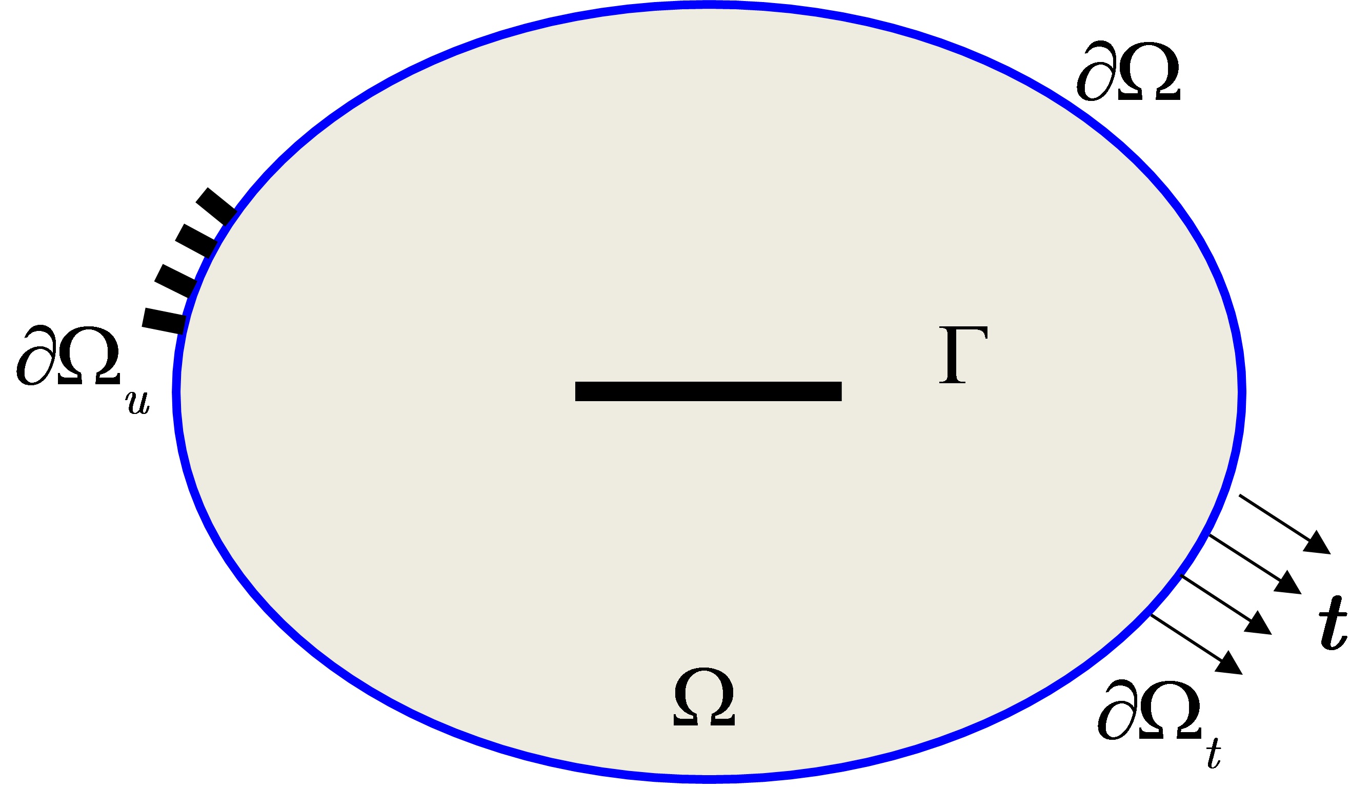
(a) Strong discontinuity

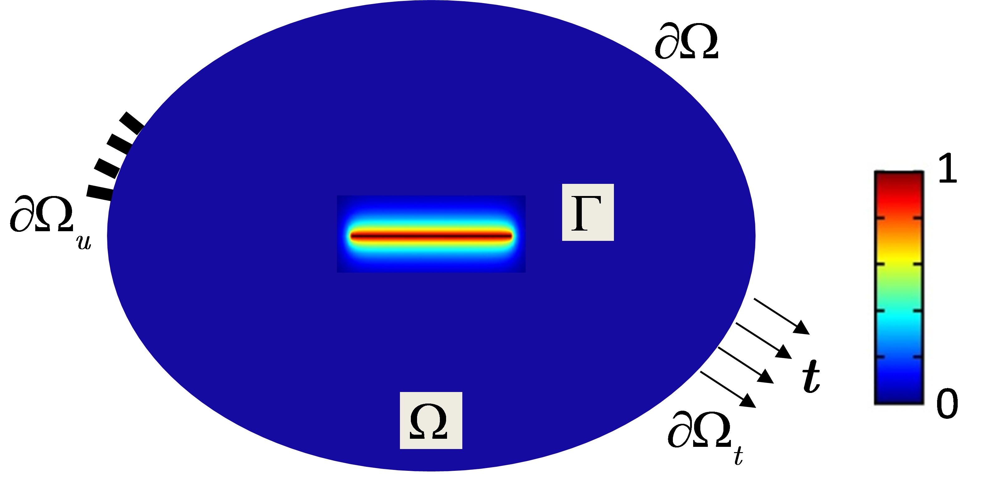
(b) Phase field representation

Figure 1: Phase field representation of discrete fractures

It should be noted that a direct application of the variational approach to fracture is difficult in numerical simulations. A leading difficulty is how to deal with the discontinuous displacement filed at fracture sets and determine the optimal fracture set. Therefore, to overcome these numerical difficulties, Bourdin et al. [57]; Miehe et al. [26] regularized the variational model by using the following energy functional $L$:

$$L=\int_{\Omega}\psi_{\varepsilon}(\bm{\varepsilon},\phi)\mathrm{d}{\Omega}+\int_{\Omega}G_{c}\left(\frac{\phi^{2}}{2l_{0}}+\frac{l_{0}}{2}|\nabla\phi|^{2}\right)\mathrm{d}\Omega-\int_{\Omega}\bm{b}\cdot{\bm{u}}\mathrm{d}{\Omega}-\int_{\partial\Omega_{t}}\bm{t}\cdot{\bm{u}}\mathrm{d}S$$ (3)

where $\phi(\bm{x},t)\in[0,1]$ ($\bm{x}$ being a position vector) is an auxiliary field, namely the phase field that is used to smear out the crack surface over the domain $\Omega$ as shown in Fig. 1b. Correspondingly, in the regularized model, the phase field $\phi(\bm{x},t)\in[0,1]$ satisfies the following conditions:

$$\phi=\begin{cases}0,\hskip 28.45274pt\text{if material is intact}\\ 1,\hskip 28.45274pt\text{if material is fully cracked}\end{cases}$$ (4)

In addition, in Eq. (3) $l_{0}$ denotes the length scale parameter which controls the transition region of the phase field. The length scale parameter thereby indirectly reflects the width of the crack. This feature has been proved by a number of numerical simulations [30; 31; 3; 33], which show that the crack region has a larger width with an increasing $l_{0}$ while the phase field will represent a sharp crack when $l_{0}$ tends to zero.

2.2 Governing equations

In a phase field method, the elastic energy can be split into different parts to model fractures of different mechanisms. For example, compressive fractures are inhibited in recent PFMs [30; 3] and to capture fractures only under tension, Miehe et al. [25] split the elastic energy into tensile and compressive parts based on the spectral decomposition of strain:

$$\bm{\varepsilon}_{\pm}=\sum_{a=1}^{d}\langle\varepsilon_{a}\rangle_{\pm}\bm{n}_{a}\otimes\bm{n}_{a}$$ (5)

where $\bm{\varepsilon}_{+}$ and $\bm{\varepsilon}_{-}$ are the tensile and compressive strain tensors, $\varepsilon_{a}$ is the principal strain, and $\bm{n}_{a}$ is the direction of the principal strain. In addition, the operators $\langle\cdot\rangle_{\pm}$ are defined as: $\langle\cdot\rangle_{\pm}=(\cdot\pm|\cdot|)/2$.

By using the strain decomposition, Miehe et al. [25] defined the elastic energy density in Eq. (3) as

$$\psi_{\varepsilon}(\bm{\varepsilon},\phi)=\left[(1-k)(1-\phi)^{2}+k\right]\psi_{\varepsilon}^{+}(\bm{\varepsilon})+\psi_{\varepsilon}^{-}(\bm{\varepsilon})$$ (6)

with the positive and negative elastic energy densities defined by

$$\psi_{\varepsilon}^{\pm}(\bm{\varepsilon})=\frac{\lambda}{2}\langle\mathrm{tr}(\bm{\varepsilon})\rangle_{\pm}^{2}+\mu\mathrm{tr}\left(\bm{\varepsilon}_{\pm}^{2}\right)$$ (7)

where $\lambda>0$ and $\mu>0$ are the Lamé constants. In this study, the Lamé constants are obtained from the Young’s modulus $E$ and Poisson’s ratio $\nu$ of the material through the well-known relation:

$$\left\{\begin{aligned} \lambda&=\frac{E\nu}{(1+\nu)(1-2\nu)}\\ \mu&=\frac{E}{2(1+\nu)}\end{aligned}\right.$$ (8)

In addition, in Eq. (6), $0<k\ll 1$ is a stability parameter for avoiding numerical singularities when the phase field $\phi$ tends to 1. Thus, by combining Eqs. (5) to (8), the regularized variational model of fracture in Eq. 3 can give rise to the governing equations with respect to the displacement $\bm{u}$ and the phase field $\phi$. Provided that the first variation of the functional $\delta L=0$ holds for all admissible displacement and phase fields, the governing equations of strong form read

$$\left\{\begin{aligned} \nabla\cdot\bm{\sigma}+\bm{b}=\bm{0}\\ \left[\frac{2l_{0}(1-k)\psi_{\varepsilon}^{+}}{G_{c}}+1\right]\phi-l_{0}^{2}\nabla^{2}\phi=\frac{2l_{0}(1-k)\psi_{\varepsilon}^{+}}{G_{c}}\end{aligned}\right.$$ (9)

where $\bm{\sigma}$ is the Cauchy stress tensor calculated by

$$\bm{\sigma} =\partial_{\bm{\varepsilon}}\psi_{\varepsilon}$$ (10)

$$=\underbrace{\left[(1-k)(1-\phi)^{2}+k\right]\left[\lambda\langle tr(\bm{\varepsilon})\rangle_{+}\bm{I}+2\mu\bm{\varepsilon}_{+}\right]}_{\bm{\sigma}^{+}}+\underbrace{\lambda\langle tr(\bm{\varepsilon})\rangle_{-}\bm{I}+2\mu\bm{\varepsilon}_{-}}_{{\bm{\sigma}}^{-}}$$

with a unit tensor $\bm{I}$ $\in\mathbb{R}^{d\times d}$.

To avoid fracture healing, Miehe et al. [26, 25] replaced the positive energy in Eq. (9) by a new driving force $H$. Note that $H=\mathrm{max}(\psi_{\varepsilon}^{+})$ is the maximum positive reference energy and it ensures the crack irreversibility [26; 25]. Therefore, a monotonically increasing phase field can be ensured with the increase of $H$, and the governing equations of strong form are rewritten as

$$\left\{\begin{aligned} \nabla\cdot\bm{\sigma}+\bm{b}=\bm{0}\\ \left[\frac{2l_{0}(1-k)H}{G_{c}}+1\right]\phi-l_{0}^{2}\nabla^{2}\phi=\frac{2l_{0}(1-k)H}{G_{c}}\end{aligned}\right.$$ (11)

subjected to the Dirichlet and Neumann boundary conditions

$$\left\{\begin{aligned} &\bm{u}=\bar{\bm{u}}\hskip 56.9055pt&\mathrm{on}\hskip 14.22636pt\partial\Omega_{u}\\ &\bm{\sigma}\cdot\bm{n}=\bm{t}&\mathrm{on}\hskip 14.22636pt\partial\Omega_{t}\\ &\nabla\phi\cdot\bm{n}=0&\mathrm{on}\hskip 14.22636pt\partial\Omega\\ \end{aligned}\right.$$ (12)

As can be seen from the equation sets in (11) and (12), the original variational problem that involves strong discontinuities is now successfully transformed to a standard multi-field problem. For solving this type of problem, conventional finite element methods can be applied, which facilities the implementation of the regularized phase field method. In addition, because the elasticity tensor is calculated by $\mathbb{D}={\partial\bm{\sigma}}/{\partial\bm{\varepsilon}}={\partial\bm{\sigma}}^{+}/{\partial\bm{\varepsilon}}+{\partial\bm{\sigma}}^{-}/{\partial\bm{\varepsilon}}$, an anisotropic constitutive relationship exists between the stress and strain and the approach in Miehe et al. [26] is hence called as an anisotropic phase field method.

3 Modified phase field model for compressive-shear fractures

3.1 Comparison on the current PFMs and their limitations

In the former section, we use the anisotropic model of Miehe et al. [26, 25] as a classical example to show the fundamental theoretical aspects in a phase field model on the basis of the variational principle. However, more generally, the PFMs for quasi-static fractures can be classified into three basic types under the framework of a regularized formulation; expect the anisotropic methods such as the model of Miehe et al. [26], the isotropic and hybrid (isotropic-anisotropic) phase field methods [53; 21; 58] are also developed according to the energy references and constitutive models used. Some representative PFMs of the isotropic, anisotropic, and hybrid forms are listed in Table 1. Note that the isotropic and anisotropic formulations are consistent with the variational principle while the hybrid ones lose fairly some thermodynamic consistency.

The three types of PFMs can be applied to capture tensile fractures in rocks, which is indicated by the formulations in Table 1. However, these PFMs have difficulties in modeling shear fractures, especially those compressive-shear fractures that are commonly observed in rock-like solids. This can be also verified through Table 1 and Fig. 2, which shows different forms of shear fractures for better comparison. In the first place, Table 1 indicates that the typical anisotropic and hybrid phase field methods cannot model the compressive-shear fractures because the compressive part of the elastic energy is not included in the driving force for the evolution equation of phase field. Therefore, only some fractures under tension-shear mode (Fig. 2b and c) can be simulated by using the anisotropic and hybrid PFMs. In the second place, although the isotropic formulations can model fractures under compression, these fractures are reported to be unrealistic [26; 25]. Furthermore, cohesion and internal friction angle are not included in the formerly developed PFMs; this is inconsistent with the experimental observations because it is generally accepted that for geomaterials the internal friction angle and cohesion have a significant effect on the compressive-shear fracture propagation and load-displacement curves [59]. Hence, a phase field model for simulating fractures in geomaterials should be able to account for the compressive-shear fractures and also to include the effects of cohesion and internal friction angle. Hence, in the following sections we will describe a new phase field model to simulate compressive-shear fractures in rock-like materials by introducing a new driving force $H_{p}$ in the evolution equation of phase field.

Table 1: Different forms of phase field methods

Type	Governing equations	Definition
Isotropic	$$\left\{\begin{aligned} &\nabla\cdot\bm{\sigma}+\bm{b}=0\\ &-l_{0}^{2}\Delta\phi+\phi=\frac{2l_{0}}{G_{c}}(1-\phi)H\\ &\bm{\sigma}(\bm{u},\phi)=(1-\phi)^{2}\frac{\partial\psi_{0}}{\partial\bm{\varepsilon}}\\ &\mathbb{D}=\frac{\partial\bm{\sigma}}{\partial\bm{\varepsilon}}\\ \end{aligned}\right.$$	$H=\max\limits_{\tau\in[0,t]}\psi_{0}\left(\bm{\varepsilon}(\bm{x},\tau)\right)$ with $\psi_{0}=\frac{\lambda}{2}(\mathrm{tr}(\bm{\varepsilon}))^{2}+\mu\mathrm{tr}(\bm{\varepsilon}^{2})$
Anisotropic [26]	$$\left\{\begin{aligned} &\nabla\cdot\bm{\sigma}+\bm{b}=0\\ &\left(\frac{2l_{0}H}{G_{c}}+1\right)\phi-l_{0}^{2}\nabla^{2}\phi=\frac{2l_{0}H}{G_{c}}\\ &\bm{\sigma}(\bm{u},\phi)=(1-\phi)^{2}\frac{\partial\psi_{\varepsilon}^{+}}{\partial\bm{\varepsilon}}+\frac{\partial\psi_{\varepsilon}^{-}}{\partial\bm{\varepsilon}}\\ &\mathbb{D}=\frac{\partial\bm{\sigma}^{+}}{\partial\bm{\varepsilon}}+\frac{\partial\bm{\sigma}^{-}}{\partial\bm{\varepsilon}}\\ \end{aligned}\right.$$	$H=\max\limits_{\tau\in[0,t]}\psi_{\varepsilon}^{+}\left(\bm{\varepsilon}(\bm{x},\tau)\right)$, $\bm{\sigma}^{+}=(1-\phi)^{2}\frac{\partial\psi_{\varepsilon}^{+}}{\partial\bm{\varepsilon}}$, $\bm{\sigma}^{-}=\frac{\partial\psi_{\varepsilon}^{-}}{\partial\bm{\varepsilon}}$, $\psi_{\varepsilon}^{\pm}(\bm{\varepsilon})=\frac{\lambda}{2}\langle\mathrm{tr}(\bm{\varepsilon})\rangle_{\pm}^{2}+\mu\mathrm{tr}\left(\bm{\varepsilon}_{\pm}^{2}\right)$
Anisotropic [60]	$$\left\{\begin{aligned} &\nabla\cdot\bm{\sigma}+\bm{b}=0\\ &-l_{0}^{2}\Delta\phi+\phi=\frac{2l_{0}}{G_{c}}(1-\phi)H\\ &\bm{\sigma}(\bm{u},\phi)=(1-\phi)^{2}\frac{\partial\psi_{0}^{+}}{\partial\bm{\varepsilon}}+\frac{\partial\psi_{0}^{-}}{\partial\bm{\varepsilon}}\\ &\mathbb{D}=\frac{\partial\bm{\sigma}^{+}}{\partial\bm{\varepsilon}}+\frac{\partial\bm{\sigma}^{-}}{\partial\bm{\varepsilon}}\\ \end{aligned}\right.$$	$H=\max\limits_{\tau\in[0,t]}\psi_{0}^{+}\left(\bm{\varepsilon}(\bm{x},\tau)\right)$, $\bm{\sigma}^{+}=(1-\phi)^{2}\frac{\partial\psi_{0}^{+}}{\partial\bm{\varepsilon}}$, $\bm{\sigma}^{-}=\frac{\partial\psi_{0}^{-}}{\partial\bm{\varepsilon}}$, $\psi_{0}^{+}=\frac{1}{2}K_{n}\langle(\mathrm{tr}(\bm{\varepsilon})\rangle_{+}^{2}+\mu(\bm{\varepsilon}^{\mathrm{dev}}:\bm{\varepsilon}^{\mathrm{dev}})$, $\psi_{0}^{-}=\frac{1}{2}K_{n}\langle(\mathrm{tr}(\bm{\varepsilon})\rangle_{-}^{2}$ with $K_{n}$ a physical parameter
Hybrid [53]	$$\left\{\begin{aligned} &\nabla\cdot\bm{\sigma}+\bm{b}=0\\ &-l_{0}^{2}\Delta\phi+\phi=\frac{2l_{0}}{G_{c}}(1-\phi)H\\ &\bm{\sigma}(\bm{u},\phi)=(1-\phi)^{2}\frac{\partial\psi_{0}}{\partial\bm{\varepsilon}}\\ &\mathbb{D}=\frac{\partial\bm{\sigma}}{\partial\bm{\varepsilon}}\\ &\forall\bm{x}:\hskip 2.84544pt\Psi_{0}^{+}<\Psi_{0}^{-}\rightarrow\phi=0\\ \end{aligned}\right.$$	$H=\max\limits_{\tau\in[0,t]}\psi_{\varepsilon}^{+}\left(\bm{\varepsilon}(\bm{x},\tau)\right)$, $\psi_{0}=\frac{\lambda}{2}(\mathrm{tr}(\bm{\varepsilon}))^{2}+\mu\mathrm{tr}(\bm{\varepsilon}^{2})$, $\psi_{\varepsilon}^{+}(\bm{\varepsilon})=\frac{\lambda}{2}\langle\mathrm{tr}(\bm{\varepsilon})\rangle_{+}^{2}+\mu\mathrm{tr}\left(\bm{\varepsilon}_{+}^{2}\right)$
Hybrid [21]	$$\left\{\begin{aligned} &\nabla\cdot\bm{\sigma}+\bm{b}=0\\ &(1-\phi)\left(\frac{H_{1}}{G_{cI}}+\frac{H_{2}}{G_{cII}}\right)-\frac{1}{2l_{0}}\phi+\frac{l_{0}}{2}\Delta\phi=0\\ &\bm{\sigma}(\bm{u},\phi)=(1-\phi)^{2}\frac{\partial\psi_{0}}{\partial\bm{\varepsilon}}\\ &\mathbb{D}=\frac{\partial\bm{\sigma}}{\partial\bm{\varepsilon}}\\ \end{aligned}\right.$$	$H_{1}=\max\limits_{\tau\in[0,t]}\lambda\langle\mathrm{tr}(\bm{\varepsilon})\rangle_{+}^{2}$, $H_{2}=\max\limits_{\tau\in[0,t]}\mu\mathrm{tr}[\langle\bm{\varepsilon}\rangle_{+}^{2}]$, $G_{cI}$ and $G_{cII}$ are the critical energy release rate of modes I and II

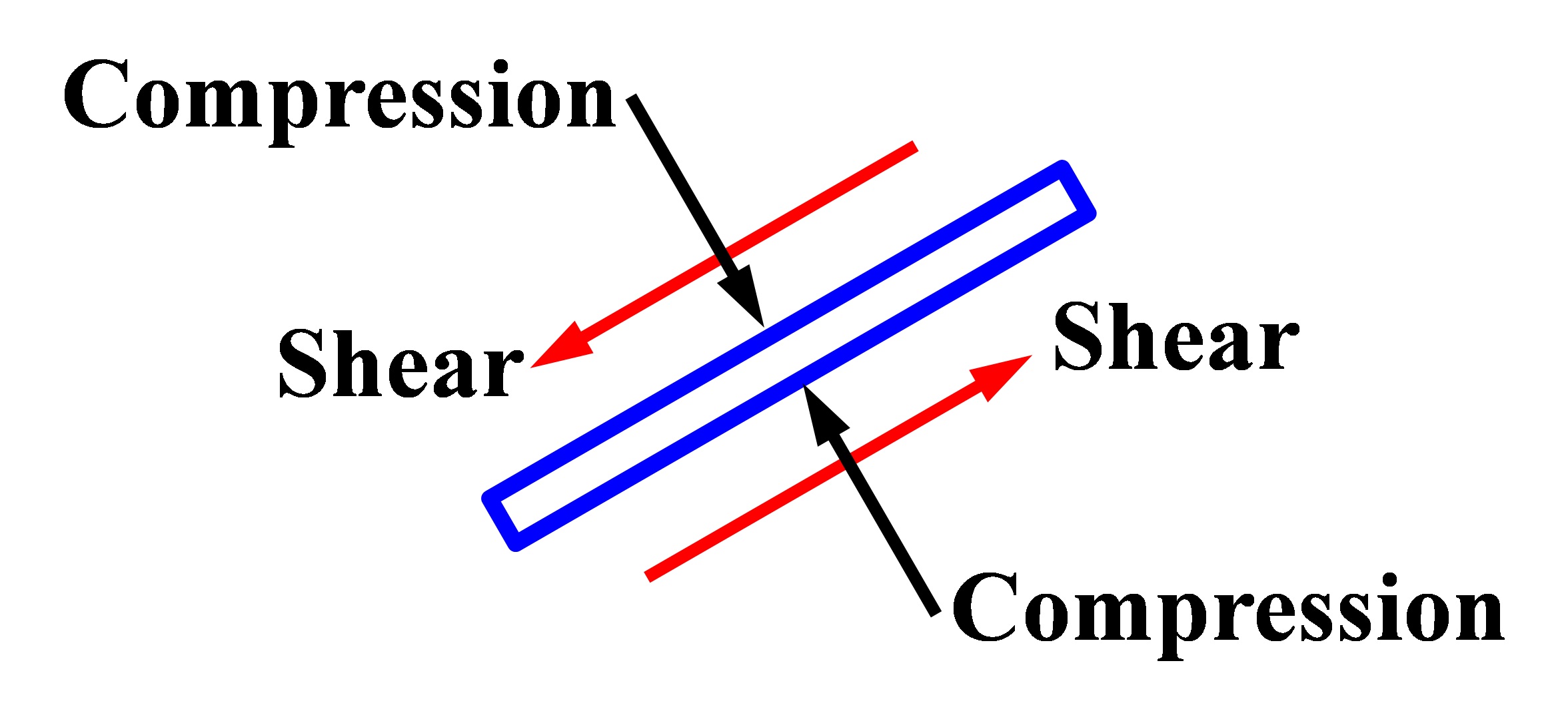
(a) Compressive-shear fracture

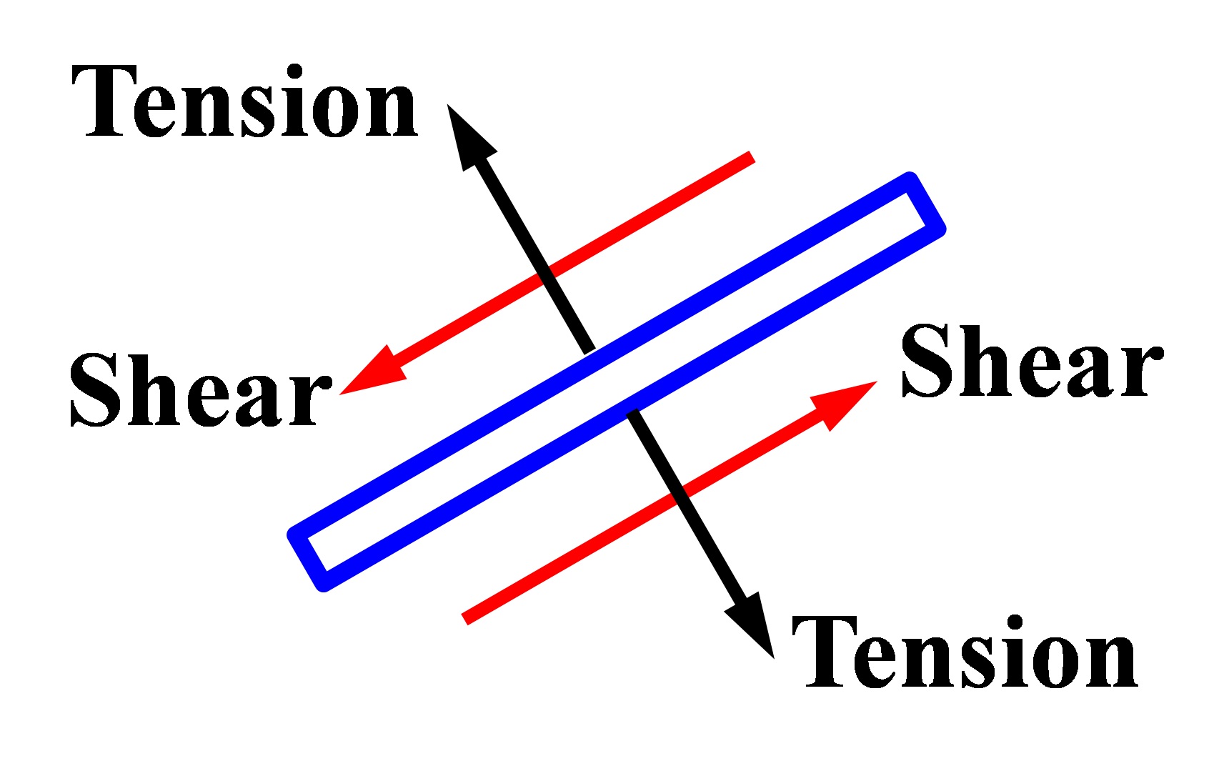
(b) Tension-shear mode

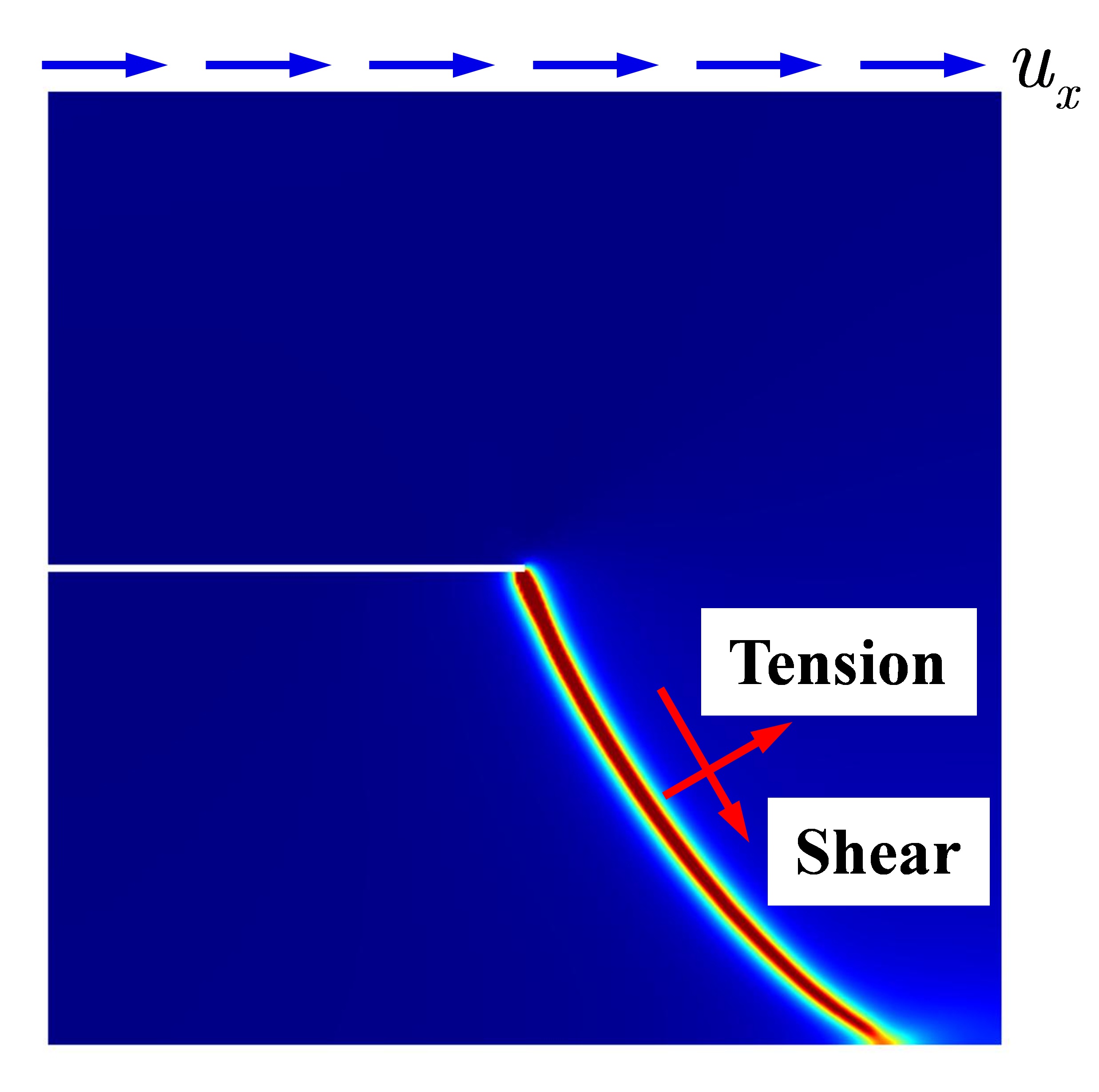
(c) Shear mode in Zhou et al. [30]

Figure 2: Different shear modes

3.2 Modified phase field model for compressive-shear fractures in rock-like solids

For rock-like materials, one way to include the effects of cohesion and internal friction angle is to apply the well-known Mohr-Coulomb criterion. However, this criterion is more suitable for macroscopic compressive-shear failure and it is a stress based failure criterion. In linear elastic fracture mechanics, the stress at crack tip is singular and is prone to exceed the strength defined by the Mohr-Coulomb criterion even when the external loads are quite small. Therefore, the macroscopically suitable Mohr-Coulomb criterion cannot be directly applied to model fracture initiation and propagation. It is also not applicable to the phase field model, which is simply an energy based method. However, many improved Mohr-Coulomb type formulations have been developed and applied in prediction of strength and damage initiation. Among these improvements are the stress level used in the statistical damage model for rocks [61; 11], and the energy based driving force to damage $w_{s}$ [62]:

$$w_{s}=\sum_{i=j+1}^{3}\sum_{j=1}^{2}\frac{1}{2G}\left(\frac{\sigma_{i}-\sigma_{j}}{2\mathrm{cos}\varphi_{ij}}+\frac{\sigma_{i}+\sigma_{j}}{2}\mathrm{tan}{\varphi_{ij}}\right)^{2}$$ (13)

where $G=\mu$ is the shear modulus, $\sigma_{i}$ and $\sigma_{j}$ are principal stresses, $\varphi_{ij}$ is the calculated angle from the Mohr diagram, and $\varphi_{13}$ is the internal friction angle. Obviously, the driving force proposed by Li et al. [62] only includes the internal friction angle while the effect of cohesion is neglected.

Given that the phase field method to fracture is an energy-driven approach, we reconstruct a new driving energy $\psi_{p}$ based on Eq. (13). For the purpose of simplicity and preventing unrealistic fractures from small shear stress, the cohesion in rock-like solids and a positive operator $\langle\centerdot\rangle_{+}$ are introduced to Eq. (13), and the energy $\psi_{p}$ is thereby written as

$$\psi_{p}=\sum_{i=j+1}^{3}\sum_{j=1}^{2}\frac{1}{2G}\left\langle\frac{\sigma_{i0}-\sigma_{j0}}{2\mathrm{cos}\varphi}+\frac{\sigma_{i0}+\sigma_{j0}}{2}\mathrm{tan}{\varphi}-c\right\rangle_{+}^{2}$$ (14)

where $c$ is the cohesion, $\varphi$ is the internal friction angle, and $\sigma_{i0}$ and $\sigma_{j0}$ are the principal stresses without including the phase field. In this study, we focus on the compressive-shear fractures. That is, the strain decomposition of Miehe et al. [26] is still applicable but only the compressive part of the principal strain is used to construct the energy in Eq. (14). Therefore, the principal stresses $\sigma_{i0}$ and $\sigma_{j0}$ are then determined by the following equation:

$$\left\{\begin{aligned} &\sigma_{i0}=\lambda\left(\varepsilon_{1p}+\varepsilon_{2p}+\varepsilon_{3p}\right)+2\mu\varepsilon_{ip}\\ &\sigma_{j0}=\lambda\left(\varepsilon_{1p}+\varepsilon_{2p}+\varepsilon_{3p}\right)+2\mu\varepsilon_{jp}\end{aligned}\right.$$ (15)

where $\varepsilon_{ip}=\langle\varepsilon_{i}\rangle_{-}$ and $\varepsilon_{jp}=\langle\varepsilon_{j}\rangle_{-}$.

By substituting Eq. (15) into Eq. (14), the energy $\psi_{p}$ is rewritten as

$$\psi_{p}=\sum_{i=j+1}^{3}\sum_{j=1}^{2}\frac{1}{2G}\left\langle\frac{\mu(\varepsilon_{ip}-\varepsilon_{jp})}{\mathrm{cos}\varphi}+\left[\lambda(\varepsilon_{1p}+\varepsilon_{2p}+\varepsilon_{3p})+\mu(\varepsilon_{ip}+\varepsilon_{jp})\right]\mathrm{tan}{\varphi}-c\right\rangle_{+}^{2}$$ (16)

To ensure the fracture irreversibility, the new driving force is defined as $H_{p}=\max\limits_{\tau\in[0,t]}\psi_{p}$. We then replace the driving force $H$ in Ambati et al. [53] by the new driving force $H_{p}$, and the governing equation set of the hybrid phase field model for simulating compressive-shear fractures in rock-like materials are thereby denoted as follows:

$$\left\{\begin{aligned} &\nabla\cdot\bm{\sigma}+\bm{b}=0\\ &\left[\frac{2l_{0}(1-k)H_{p}}{G_{c}}+1\right]\phi-l_{0}^{2}\nabla^{2}\phi=\frac{2l_{0}(1-k)H_{p}}{G_{c}}\\ &\bm{\sigma}(\bm{u},\phi)=\left[(1-k)(1-\phi)^{2}+k\right]\frac{\partial\psi_{0}}{\partial\bm{\varepsilon}}\\ &\mathbb{D}=\frac{\partial\bm{\sigma}}{\partial\bm{\varepsilon}}\\ \end{aligned}\right.$$ (17)

in which $G_{c}$ accordingly refers to the critical energy release rate of mode II. It should be noted that the proposed hybrid phase field model for compressive-shear fractures can account for the influence of internal friction angle and cohesion on initiation and propagation of fractures as well as the load-displacement curves of rock-like specimens. This important feature will be further verified in the numerical examples presented in Section 5.

4 Numerical implementation

Most of the PFMs are solved within the framework of conventional finite element methods (FEMs), and there are two different approaches at moment for coupling the displacement or other physical field with the phase field, namely the monolithic [25; 63] and staggered ones [64; 60; 26; 65; 29; 63; 58; 30; 3]. In this study, the weak forms of the governing equations (17) are first given by

$$\int_{\Omega}\bm{\sigma}:\delta\bm{\varepsilon}\mathrm{d}\Omega=\int_{\Omega}\bm{b}\cdot\delta\bm{u}\mathrm{d}\Omega+\int_{\Omega_{h}}\bm{t}\cdot\delta\bm{u}\mathrm{d}S$$ (18)

and

$$\int_{\Omega}-2(1-k)H_{p}(1-\phi)\delta\phi\mathrm{d}\Omega+\int_{\Omega}G_{c}\left(l_{0}\nabla\phi\cdot\nabla\delta\phi+\frac{1}{l_{0}}\phi\delta\phi\right)\mathrm{d}\Omega=0$$ (19)

We use the standard vector-matrix notation and the displacement and phase field are discretized as

$$\bm{u}=\mathbf{N_{u}}\mathbf{d},\hskip 14.22636pt\phi=\mathbf{\bm{N}_{\phi}}\hat{\bm{\phi}}$$ (20)

where $\mathbf{d}$ and $\hat{\bm{\phi}}$ are the constructed vectors comprising the node values $\bm{u}_{i}$ and $\phi_{i}$. In addition, the shape function matrices $\mathbf{N_{u}}$ and $\mathbf{N_{\phi}}$ in 2D are defined as

$$\mathbf{N_{u}}=\left[\begin{array}[]{ccccc}N_{1}&0&\dots&N_{n}&0\\ 0&N_{1}&\dots&0&N_{n}\end{array}\right],\hskip 14.22636pt\mathbf{N_{\phi}}=\left[\begin{array}[]{cccc}N_{1}&N_{2}&\dots&N_{n}\end{array}\right]$$ (21)

where $n$ is the node number in one element and $N_{i}$ is the shape function at node $i$. The test functions are then assumed to have the same discretization:

$$\delta\bm{u}=\mathbf{N_{u}}\delta\mathbf{d},\hskip 14.22636pt\delta\phi=\mathbf{N_{\phi}}\delta\hat{\bm{\phi}}$$ (22)

where $\delta\mathbf{d}$ and $\delta\hat{\bm{\phi}}$ are the vectors composed of the node values of the test functions.

The gradients of the trial and test functions are defined as follows,

$$\bm{\varepsilon}=\mathbf{B_{u}}\mathbf{d},\hskip 14.22636pt\nabla\phi=\mathbf{B_{\phi}}\hat{\bm{\phi}},\hskip 14.22636pt\bm{\delta}\varepsilon=\mathbf{B_{u}}\delta\mathbf{d},\hskip 14.22636pt\nabla\phi=\mathbf{B_{\phi}}\delta\hat{\bm{\phi}}$$ (23)

where $\mathbf{B_{u}}$ and $\mathbf{B_{\phi}}$ are the derivatives of the shape functions defined by

$$\mathbf{B_{u}}=\left[\begin{array}[]{ccccc}N_{1,x}&0&\dots&N_{n,x}&0\\ 0&N_{1,y}&\dots&0&N_{n,y}\\ N_{1,y}&N_{1,x}&\dots&N_{n,y}&N_{n,x}\end{array}\right],\hskip 5.69046pt\mathbf{B_{\phi}}=\left[\begin{array}[]{cccc}N_{1,x}&N_{2,x}&\dots&N_{n,x}\\ N_{1,y}&N_{2,y}&\dots&N_{n,y}\end{array}\right]$$ (24)

The equations of weak form (18) and (19) are subsequently written as

$$(\delta\mathbf{d})^{\mathrm{T}}\left[\int_{\Omega}\mathbf{B_{u}}^{\mathrm{T}}\mathbf{D_{e}}\mathbf{B_{u}}\mathrm{d}\Omega\mathbf{d}\right]=(\delta\mathbf{d})^{\mathrm{T}}\left[\int_{\Omega}\mathbf{N_{u}}^{\mathrm{T}}\bm{b}\mathrm{d}\Omega+\int_{\Omega_{h}}\mathbf{N_{u}}^{\mathrm{T}}\bm{t}\mathrm{d}S\right]$$ (25)

$$-(\delta\hat{\bm{\phi}})^{\mathrm{T}}\int_{\Omega}\left\{\mathbf{B_{\phi}}^{\mathrm{T}}G_{c}l_{0}\mathbf{B_{\phi}}+\mathbf{N_{\phi}}^{\mathrm{T}}\left[\frac{G_{c}}{l_{0}}+2(1-k)H_{p}\right]\mathbf{N_{\phi}}\right\}\mathrm{d}\Omega\hat{\bm{\phi}}+(\delta\hat{\bm{\phi}})^{\mathrm{T}}\int_{\Omega}2(1-k)H_{p}\mathbf{N_{\phi}}^{\mathrm{T}}\mathrm{d}\Omega=0$$ (26)

Equations (25) and (26) always hold for arbitrary admissible test functions, therefore, the discrete weak form equations read

$$-\underbrace{\int_{\Omega}\mathbf{B_{u}}^{\mathrm{T}}\mathbf{D_{e}}\mathbf{B_{u}}\mathrm{d}\Omega\mathbf{d}}_{\bm{F}_{u}^{int}=\bm{K}_{u}\mathbf{d}}+\underbrace{\int_{\Omega}\mathbf{N_{u}}^{\mathrm{T}}\bm{b}\mathrm{d}\Omega+\int_{\Omega_{h}}\mathbf{N_{u}}^{\mathrm{T}}\bm{t}\mathrm{d}S}_{\bm{F}_{u}^{ext}}=0$$ (27)

$$-\underbrace{\int_{\Omega}\left\{\mathbf{B_{\phi}}^{\mathrm{T}}G_{c}l_{0}\mathbf{B_{\phi}}+\mathbf{N_{\phi}}^{\mathrm{T}}\left[\frac{G_{c}}{l_{0}}+2(1-k)H_{p}\right]\mathbf{N_{\phi}}\right\}\mathrm{d}\Omega\hat{\bm{\phi}}}_{\bm{F}_{\phi}^{int}=\bm{K}_{\phi}\hat{\bm{\phi}}}+\underbrace{\int_{\Omega}2(1-k)H_{p}\mathbf{N_{\phi}}^{\mathrm{T}}\mathrm{d}\Omega}_{\bm{F}_{\phi}^{ext}}=0$$ (28)

where $\bm{F}_{u}^{int}$ and $\bm{F}_{u}^{ext}$ are the internal and external forces for the displacement field, and $\mathbf{D_{e}}$ is the degraded elasticity matrix. $\bm{F}_{\phi}^{int}$ and $\bm{F}_{\phi}^{ext}$ are the internal and external force terms of the phase field [30]. In addition, the stiffness matrices of the displacement and phase fields read

$$\left\{\begin{aligned} \bm{K}_{u}&=\int_{\Omega}\mathbf{B_{u}}^{\mathrm{T}}\mathbf{D_{e}}\mathbf{B_{u}}\mathrm{d}\Omega\\ \bm{K}_{\phi}&=\int_{\Omega}\left\{\mathbf{B_{\phi}}^{\mathrm{T}}G_{c}l_{0}\mathbf{B_{\phi}}+\mathbf{N_{\phi}}^{\mathrm{T}}\left[\frac{G_{c}}{l_{0}}+2(1-k)H_{p}\right]\mathbf{N_{\phi}}\right\}\mathrm{d}\Omega\end{aligned}\right.$$ (29)

Finally, Eqs. (27) and (28) are solved by using a staggered scheme because it provides greater flexibility as well as stability in solving the displacement and phase field compared with the monolithic scheme. The phase field and displacement are thereby solved sequentially with iterations in between. More details about the widely used staggered scheme for phase field modeling can be referred to Miehe et al. [26, 25]. We use the implicit Generalized-$\alpha$ method for time integration and the Anderson acceleration technology for increasing the convergence rate in the simulations [30; 31; 3; 32].

5 Numerical examples

In this section, some benchmark examples are tested to show the capability of the proposed PFM for brittle compressive-shear fractures in rock-like materials. These examples include uniaxial compression tests on intact rock-like specimen as well as those specimens with a single or double inclined pre-existing flaws.

5.1 An intact specimen under uniaxial compression

In this example, we test the compressive-shear fractures in an intact prism specimen subjected to axial compression, and 2D plane strain and 3D simulations are performed. Geometry and boundary conditions of the specimen are shown in Fig. 3a. We apply vertical displacement on the upper end of the specimen. To reduce complexity of this numerical test, we only introduce a random distribution on the Young’s modulus of the specimen for the purpose of inducing a non-uniform stress field, which will further drives the fracture propagation in part of the specimen without producing everywhere identical phase field in the specimen. In this example, the Young’s modulus $E(\bm{x})$ is assumed to follow Weibull distribution [11; 66] and the corresponding probability density function $p$ is expressed as follows,

$$p(E)=\frac{m}{E_{0}}\left(\frac{E}{E_{0}}\right)^{m-1}\mathrm{exp}\left[-\left(\frac{E}{E_{0}}\right)^{m}\right]$$ (30)

where $E_{0}$ is the mean value of the Young’s modulus and $m$ is a parameter that defines the shape of Weibull distribution (see also different density curves about Weibull distribution under different $m$ in Zhou et al. [11]).

The resulting Young’s modulus distribution is shown in Fig. 3b and c. The mean value of $E$ is 90 GPa for both 2D and 3D while the maximum and minimum values are 903 GPa and 0.45 MPa in 2D, and the maximum and minimum values for 3D are 883 GPa and 0.431 MPa, respectively. The other parameters are chosen as $\nu=0.3$, $G_{c}=6$ N/m, $m=1$, $l_{0}=1$ mm, $\varphi=20^{\circ}$, and $c=100$ kPa; these parameters are used for both 2D and 3D calculation for an intact rock specimen and are obtained from the experimental results (stress-strain curve of the first sample) in Xia et al. [9]. Note that we apply the initial Young’s modulus of the rock specimen in the actual experimental test in the phase field modeling. In 2D simulation, a total of 16,000 regular Q4 elements with characteristic size of $h=0.5$ mm are used to discretize the specimen while 6-node prism elements with maximum element size $h=1$ mm are applied for 3D and $k=1\times 10^{-9}$ is selected to prevent numerical singularity. In each time step, we set the displacement increment as $\Delta u=2\times 10^{-6}$ mm.

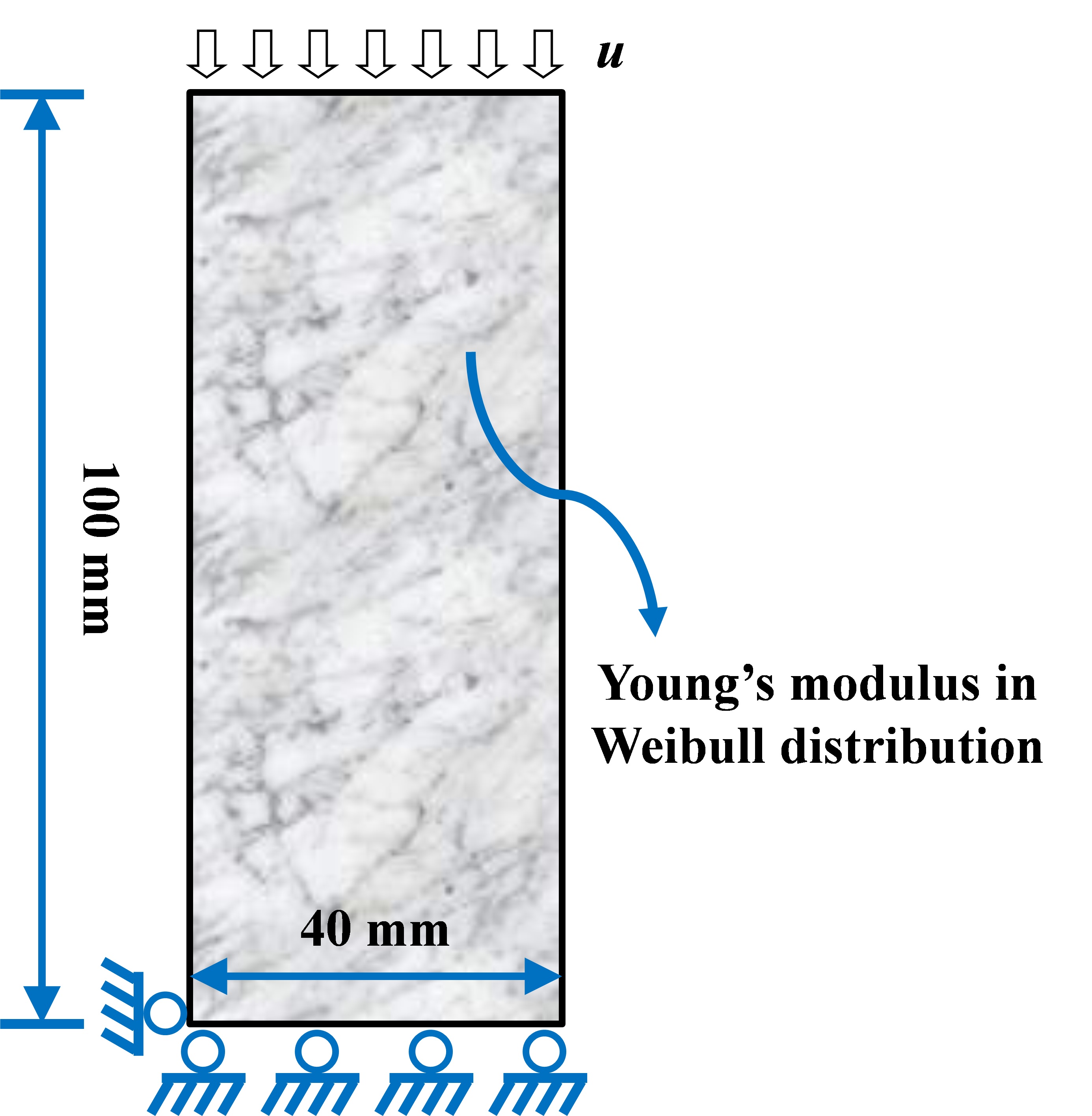
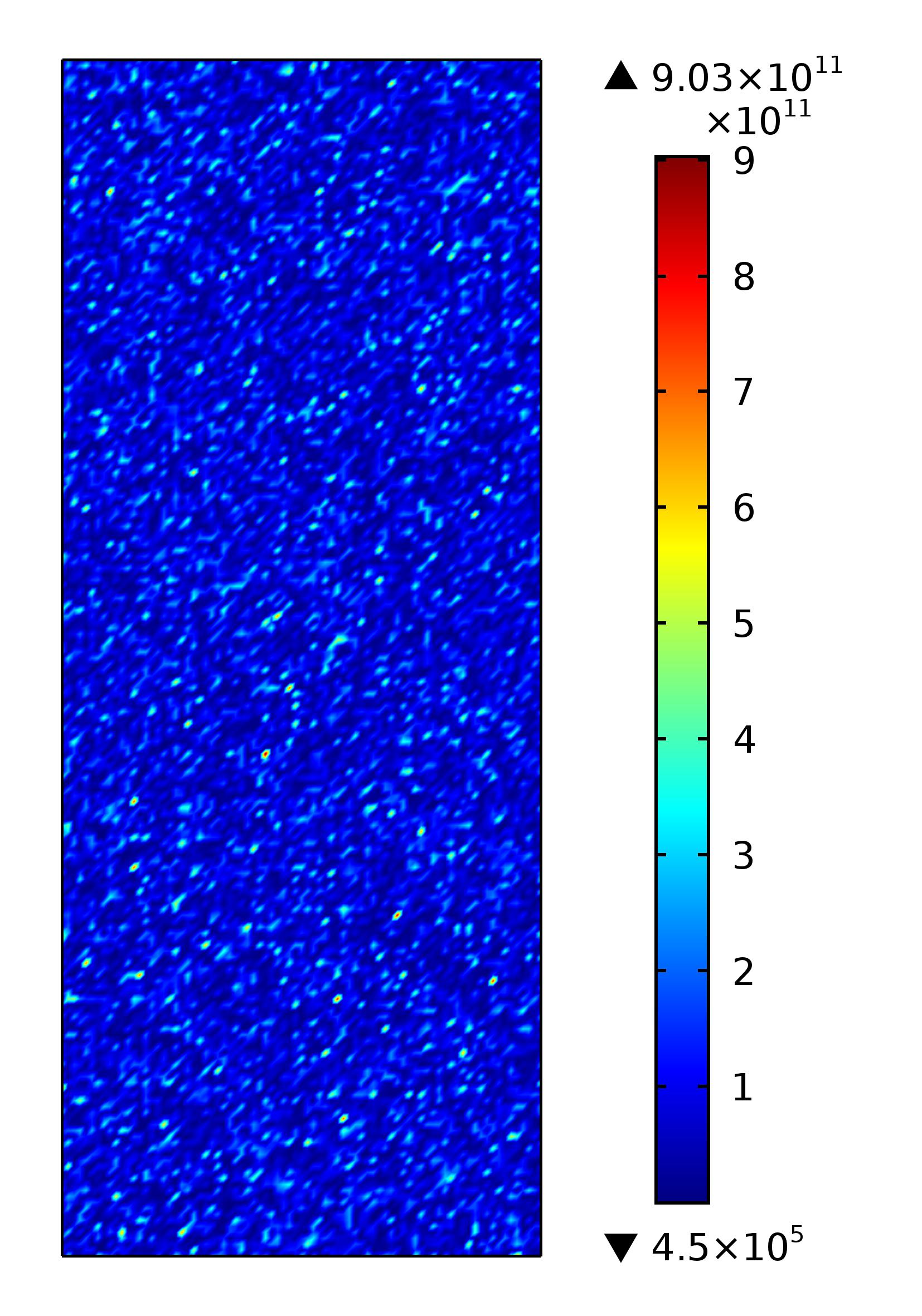
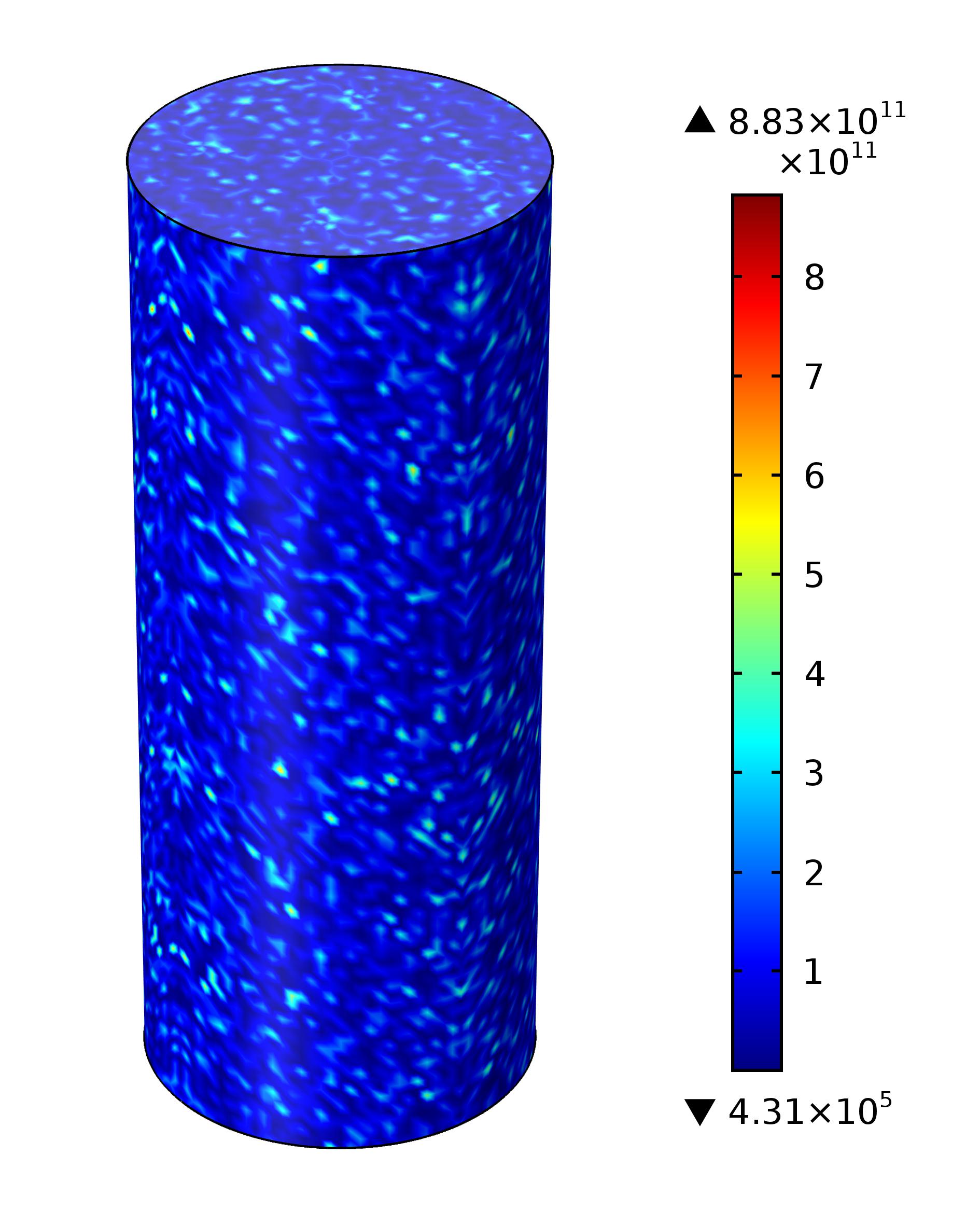
Figure 3: An intact rectangular specimen subjected to uniaxial compression. (a) Geometry and boundary conditions, (b) distribution of Young’s modulus in 2D (Unit: Pa), and (c) distribution of Young’s modulus in 3D (Unit: Pa)

Figure 4 shows the phase field contour plot of the intact specimen at different displacements. As can be seen in Fig. 4a, the phase field is randomly distributed and its maximum value occurs at the lower left corner of the specimen. On the other hand, Fig. 4b displays the final fracture pattern for 2D. A V-shaped compressive-shear fracture forms in Fig. 4b with the increasing axial compressive load. For 3D, Fig. 4c also shows a V-shaped fracture pattern. The 2D and 3D phase field simulations in this study agree well with the experimental observations where the V-shaped compressive-shear fracture pattern is the most frequently observed in experimental tests. Some representative examples of the V-shaped shear fracture can be seen in Fig. 5. Note that the fracture type in basalt (Fig. 5a) comes from the sample OR1 in Xia et al. [9] and the compressive-shear fractures were observed in cement mortar (Fig. 5b) while the fractures in sandstones in Fig. 5c and d are obtained in Basu et al. [8].

(a) $u=0.92$ mm, 2D

(b) $u=0.9215$ mm, 2D

(c) $u=0.104$ mm, 3D

Figure 4: Phase field of the intact specimen at different displacements

(a) Basalt [9]

(b) Cement mortar

(c) Sandstone [8]

(d) Sandstone [8]

Figure 5: Experimental observations of the V-shaped compressive-shear fractures

Figure 6 compares the stress-strain curves obtained by the phase field simulation and the experimental tests (sample OR1 in Xia et al. [9]). In this figure, the stress refers to the averaged pressure on the upper boundary of the specimen and the strain refers to the ratio of the displacement on the upper end to the height of the specimen. As observed, the proposed PFM achieves a close stress-strain curve to the experimental test and as expected the 3D PFM agrees better to the experiment than 2D plane strain model. The 2D PFM obtains a stress-strain curve with a slight deviation from the experimental curve because 2D plane strain assumption provides extra stiffness for the vertical direction due to the displacement restriction perpendicular to the plane. Therefore, for an intact specimen, the proposed phase field model can exactly reproduce the fracture pattern and stress-strain curve, which preliminarily indicates the effectiveness of the proposed PFM for compressive-shear fractures.

Figure 6: Comparison of the stress-strain curves of the phase field simulation and experimental tests

5.2 Uniaxial compression of a specimen with an inclined flaw

The fractures caused by uniaxial compression on rock-like materials with an inclined flaw have been widely investigated both experimentally and numerically (see some typical contributions in Lajtai [4]; Ingraffea and Heuze [68]; Wong and Einstein [6]; Yang and Jing [7]; Zhuang et al. [69]; Zhang et al. [21] and these literature applied cuboid or cubic rock specimens). Therefore, in this example, we apply the proposed PFM to simulate the compressive-shear fractures in a rectangular specimen with an inclined flaw subjected to axial compression. The setup of the problem including the geometry and boundary conditions is illustrated in Fig. 7 along with the width and height of the rock-like specimen being 50 mm and 100 mm, respectively. The flaw is 5 mm in length and 1 mm in width; its center is located in the axis of symmetry and deviates from the center of the specimen by an eccentricity $e$. Moreover, the pre-existing flaw is inclined at an angle $\alpha$ to the horizontal direction, and a vertical downward displacement is applied on the upper end of the specimen.

Figure 7: Setup of a rectangular specimen with an inclined flaw subjected to uniaxial compression

These base parameters are used for calculation: inclination angle $\alpha=45^{\circ}$, Young’s modulus $E$ = 60 GPa, Poisson’s ratio $\nu$ = 0.3, critical energy release rate $G_{c}$ = 100 N/m, length scale parameter $l_{0}$ = 1 mm, $k=1\times 10^{-9}$, cohesion $c$ = 100 kPa, and internal friction angle $\varphi=15^{\circ}$. According to Zhang et al. [67], the length scale used in this example can capture accurate crack paths since the ratio of the length scale to the specimen size is sufficiently small. A total of 51906 triangular elements are used to discretize the domain with the maximum element size $h$ = 0.5 mm. In addition, we adopt a displacement increment $\Delta u=1\times 10^{-4}$ mm in the simulations.

For an inclination angle of the flaw $\alpha=45^{\circ}$, the progressive fracture patterns obtained by the proposed phase field model are shown in Fig. 8. It can be seen from Fig. 8a that with the increase in the compressive loads, shear zones occur around the tips of the inclined flaw, and that two new fractures initiate at the flaw tips due to the increasing energy reference $H_{p}$, the evolution of which is shown in Fig 9. As shown in Fig. 8b, when the displacement on the upper boundary of the specimen increases to $0.1554$ mm, the fractures propagate obliquely and become wider because of complex compressive-shear zones around the fractures. In addition, Fig. 8c indicates that when $u=0.1558$ mm the fractures continue propagating at an increasing angle to the horizontal direction; finally an inclined fracture pattern is observed.

In an experimental test of uniaxial compression on rock-like materials with a flaw of $\alpha=45^{\circ}$, some salient features about the compressive-shear fracture responses can be observed and further classified into two categories: the normal and inclined shear fractures [4; 6]. These two types can be seen in Figs. 10 and 11, which interpret the experimental results of the compressive-shear fractures in square and rectangular specimens respectively, although the fractures are named a lateral fracture and a pure shear fracture by Yang and Jing [7]. Comparing Figs. 8, 10, and 11 show that the compressive-shear fractures modeled by the proposed PFM are consistent with the experimental results.

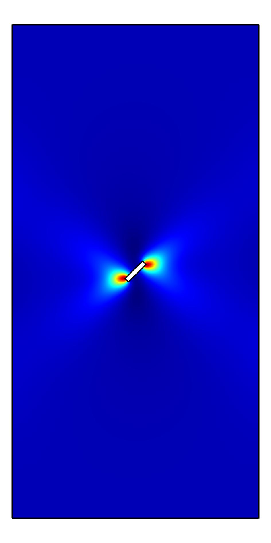
(a) $u=0.1540$ mm

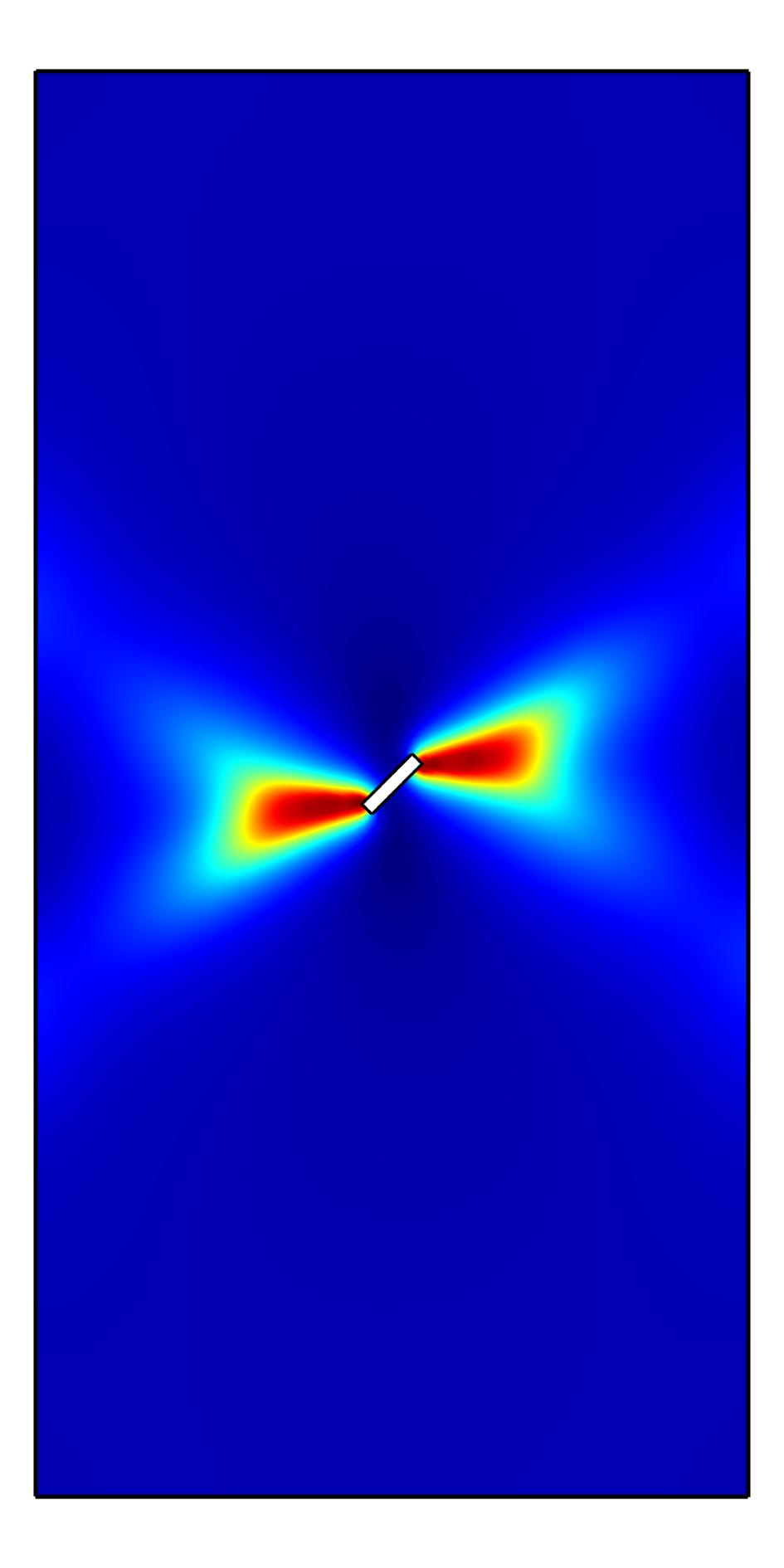
(b) $u=0.1554$ mm

(c) $u=0.1558$ mm

Figure 8: Fracture patterns of a specimen with an inclined flaw ($\alpha=45^{\circ}$)

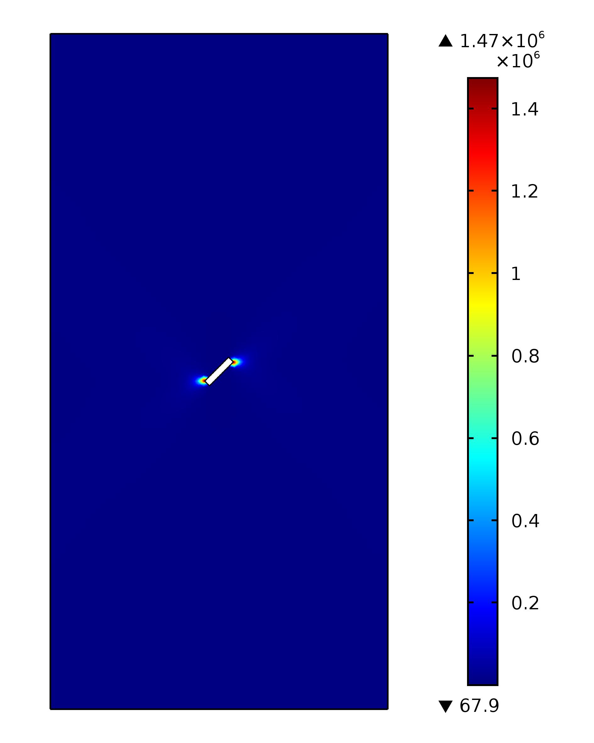
(a) $u=0.1540$ mm

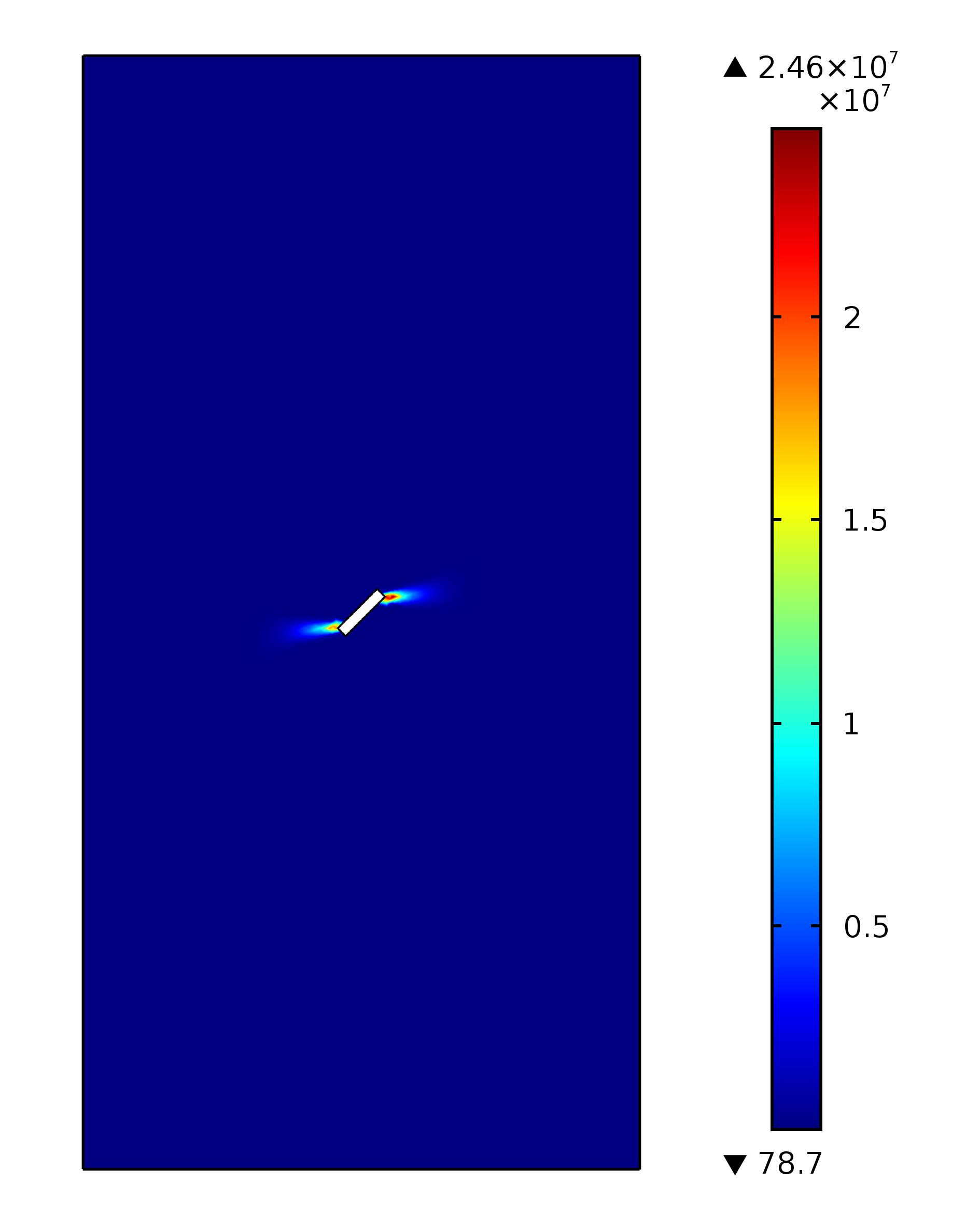
(b) $u=0.1554$ mm

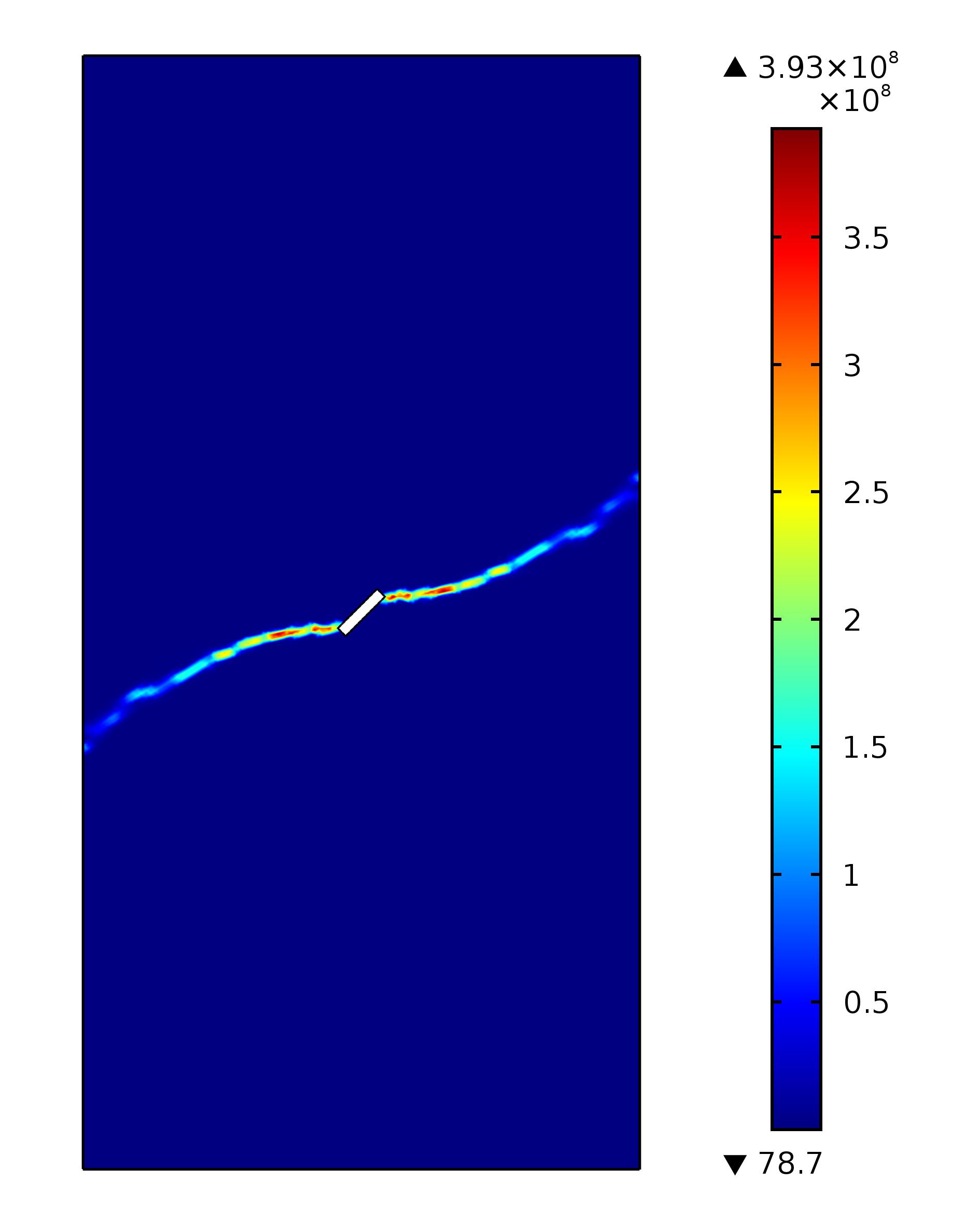
(c) $u=0.1558$ mm

Figure 9: Evolution of $H_{p}$ for a specimen with an inclined flaw ($\alpha=45^{\circ}$) (Unit:J/m³)

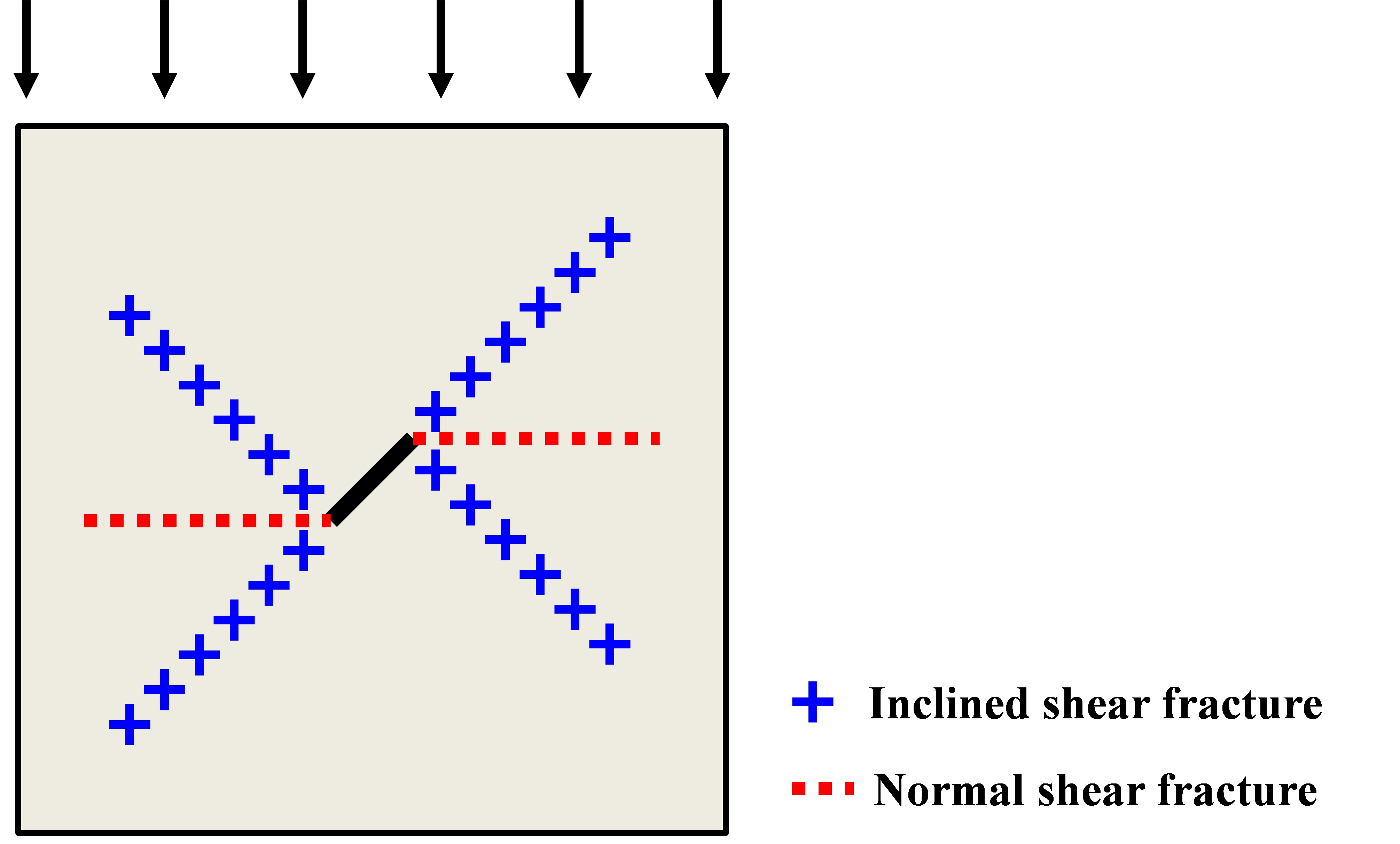
Figure 10: A specimen with an inclined flaw ($\alpha=45^{\circ}$). Experimental observations of the compressive-shear fractures in Lajtai [4]; Wong and Einstein [6]

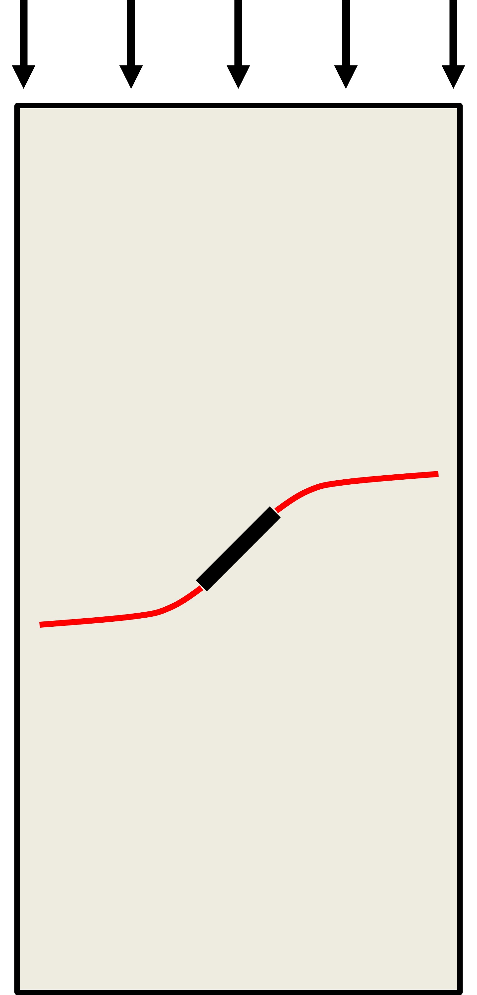
(a) Lateral fractures

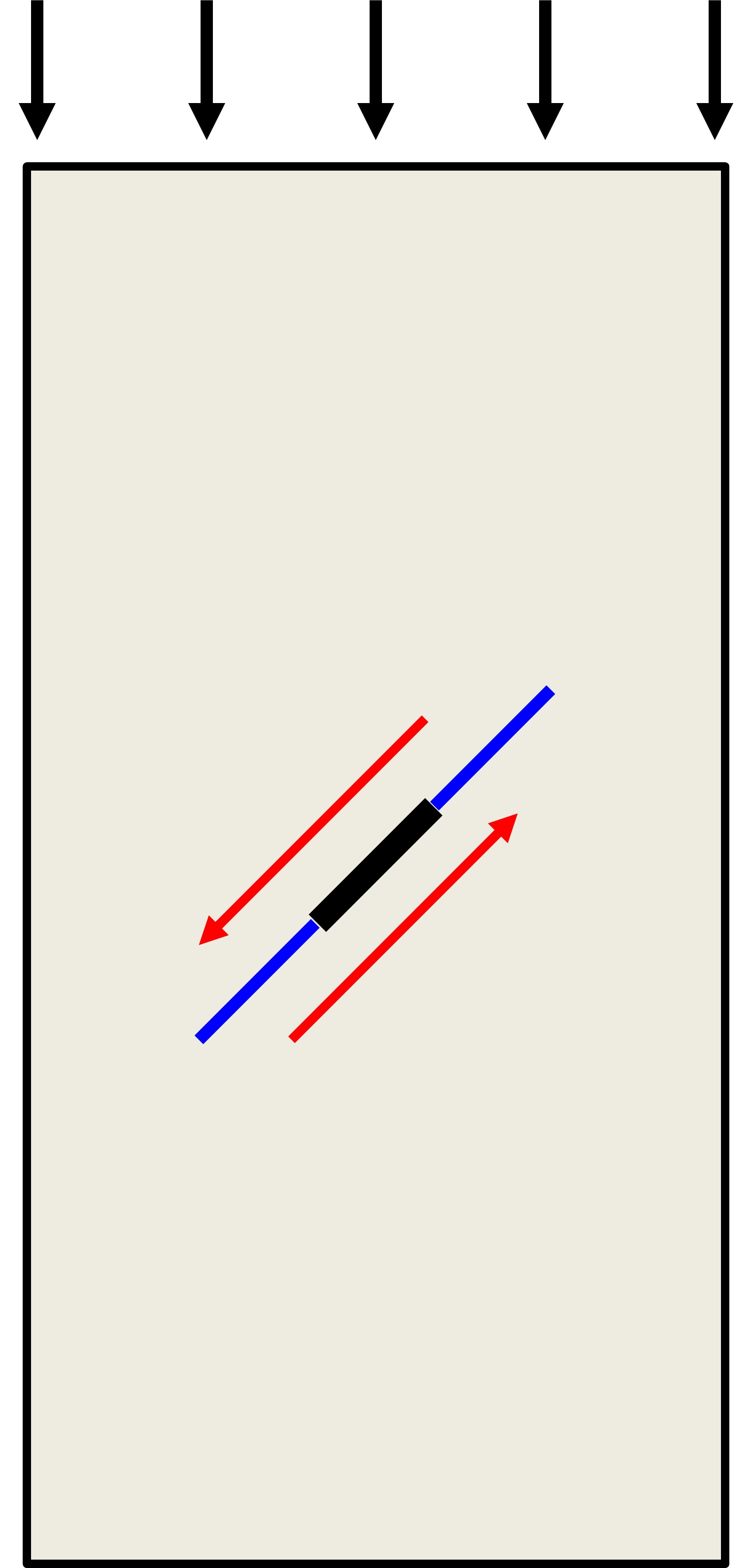
(b) Pure shear fractures

Figure 11: Experimental observations of the compressive-shear fractures for a specimen with an inclined flaw ($\alpha=45^{\circ}$) in Yang and Jing [7]

We also compare the fracture pattern and load-displacement curves obtained by our model and the anisotropic model [25] in Fig. 12. Note that both models are tested under the same parameters. In Fig. 12, the anisotropic model of [25] is found to not have a drop stage in the load-displacement curve while the drop stage in our model is obvious. Moreover, only wing and anti-wing tensile cracks are simulated in the model of [25]. Therefore, the comparison in Fig. 12 convinces the finding that the anisotropic PFM is not suitable for predicting compressive-shear fracture in rock-like materials.

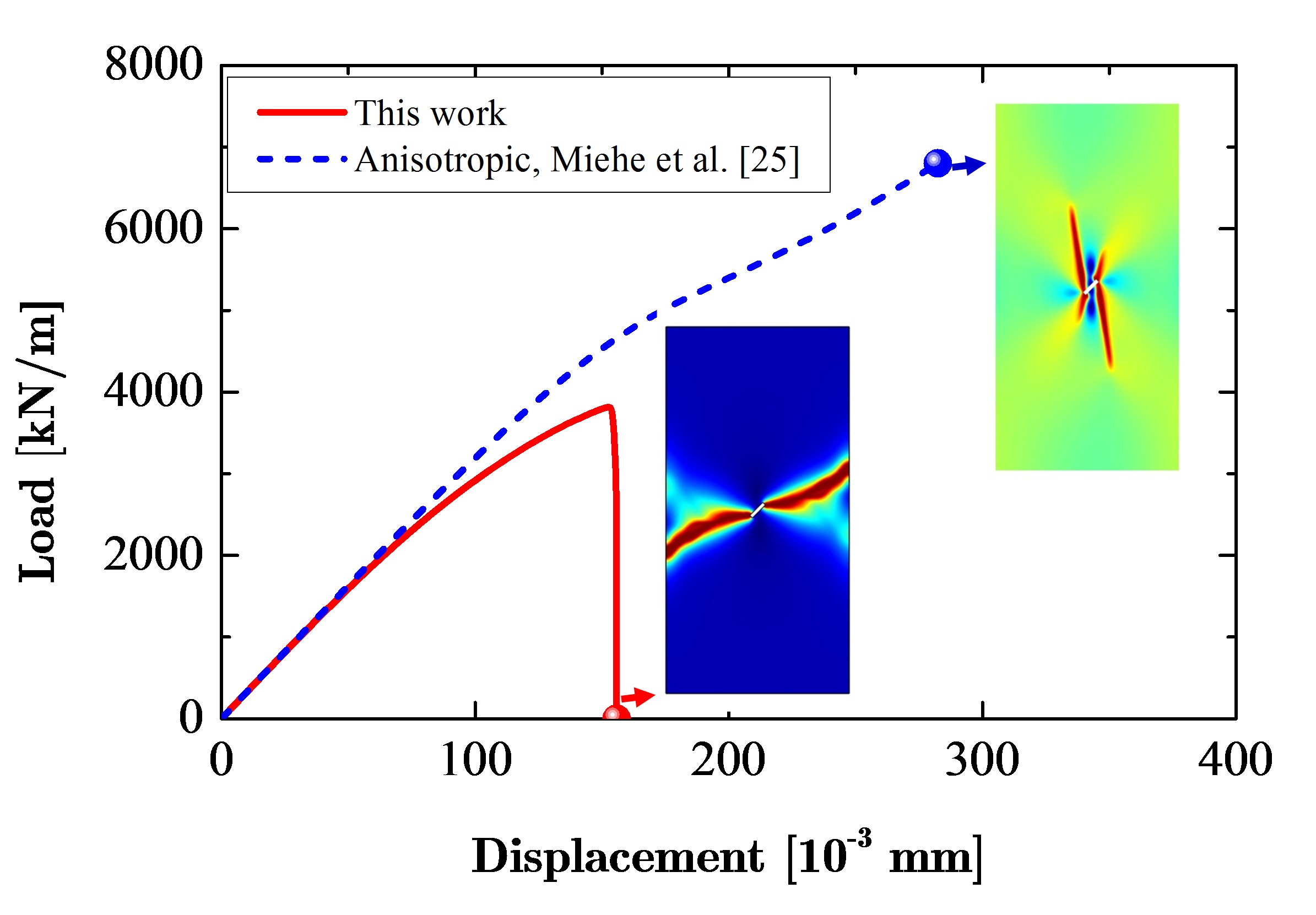
Figure 12: Comparison of fracture pattern and load-displacement curve obtained by the proposed PFM and the anisotropic model of [25]

We then test the influence of the inclination angle $\alpha$ on the compressive-shear fracture patterns. The inclination angle varies from $0^{\circ}$, $15^{\circ}$, $30^{\circ}$, $60^{\circ}$, $75^{\circ}$, to $90^{\circ}$ while the other parameters remain unchanged. For $\alpha$ = $15^{\circ}$, $30^{\circ}$, $60^{\circ}$, and $75^{\circ}$, the progressive fracture process is similar to that for $\alpha=45^{\circ}$. All the modeled fractures in these cases belong to the inclined shear fractures. However, for $\alpha=0^{\circ}$ and $90^{\circ}$, the fracture patterns are different from $\alpha=45^{\circ}$ because of the presence of symmetry. Figures 13 and 14 show the fracture process when $\alpha=0^{\circ}$ and $90^{\circ}$. For $\alpha=0^{\circ}$, fractures initiate at the flaw tips when $u=0.1378$ mm. Subsequently, the fractures propagates horizontally and fall into the category of normal shear fracture when $u=0.1400$ mm. However, when $u=0.1406$ mm, the propagating fractures approach the left and right boundaries and a slight fracture branching is shown in the specimen; this phenomenon is more obvious for $\alpha=90^{\circ}$. Differently from $\alpha=0^{\circ}$, fractures initiate in the middle of the flaw for $\alpha=90^{\circ}$ when $u=0.1976$ mm. Fractures start to branch when $u=0.1980$ mm and the bifurcated fractures reach the left and right boundaries when $u=0.1981$ mm. It should be noted that the modeled X-shaped fracture is in good agreement with the experimental observed pattern in Fig. 15, and it is named the double shear fracture in Basu et al. [8].

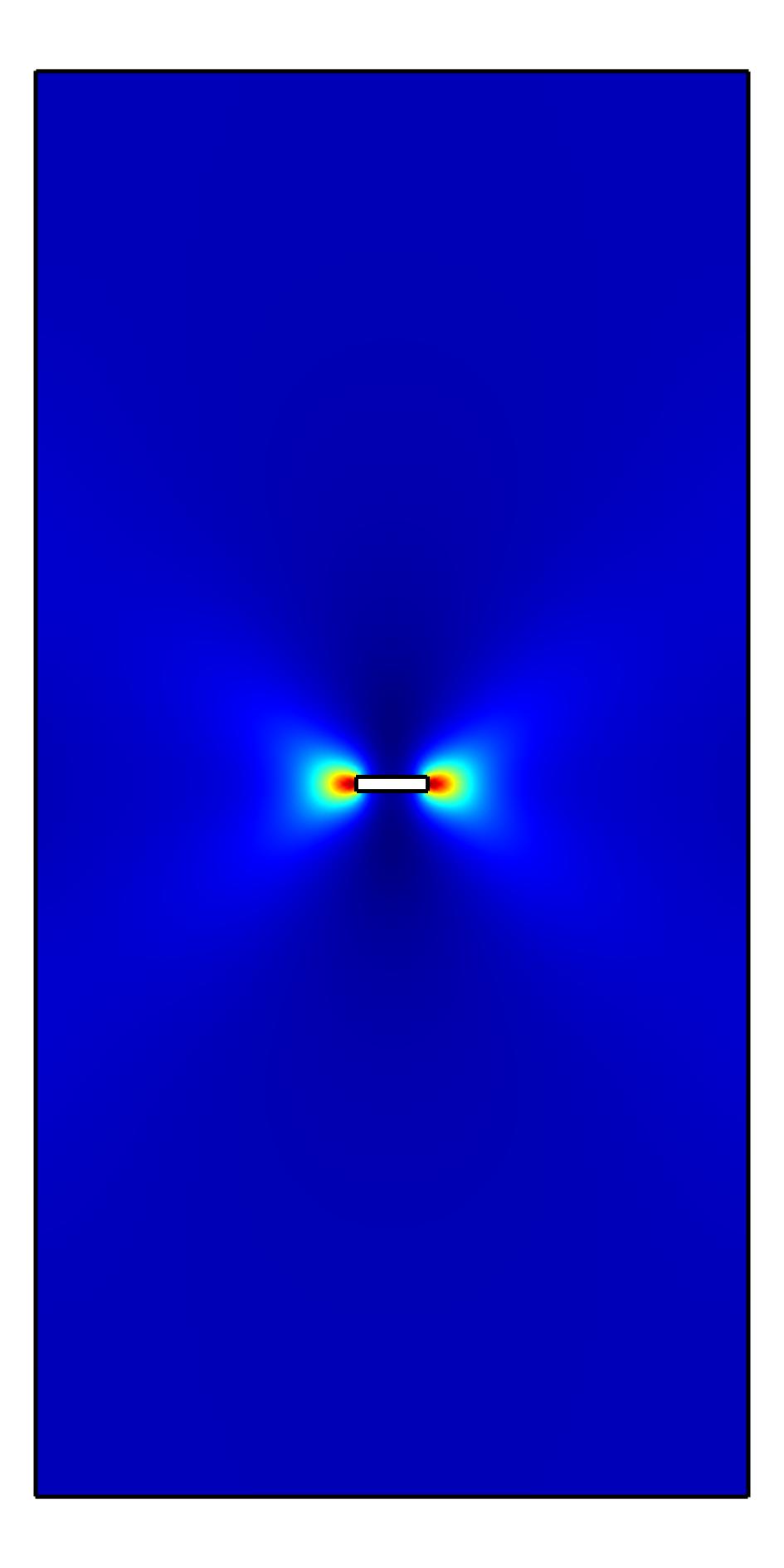
(a) $u=0.1378$ mm

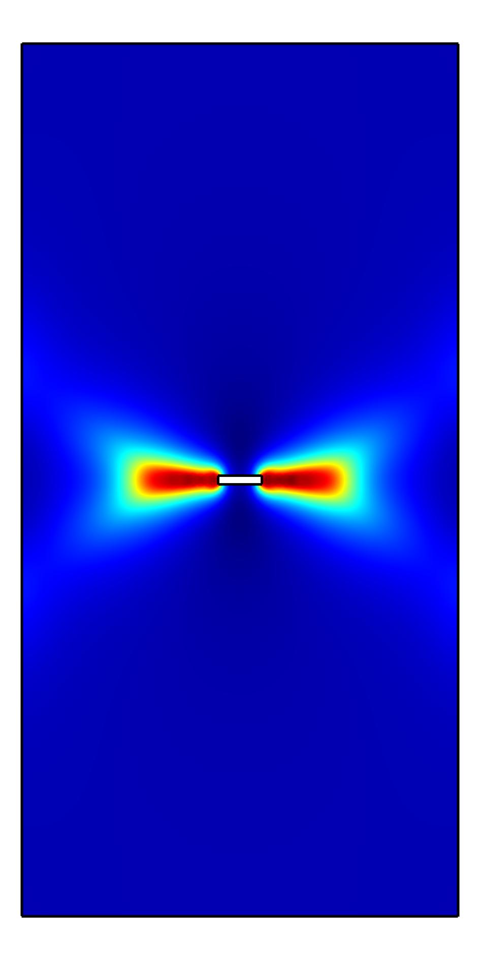
(b) $u=0.1400$ mm

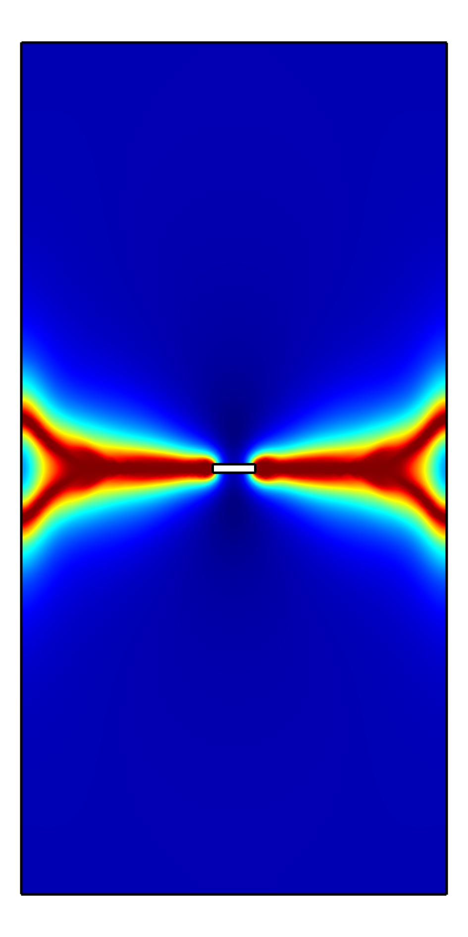
(c) $u=0.1406$ mm

Figure 13: Fracture patterns (phase field evolution) of a specimen with an inclined flaw of $\alpha=0^{\circ}$

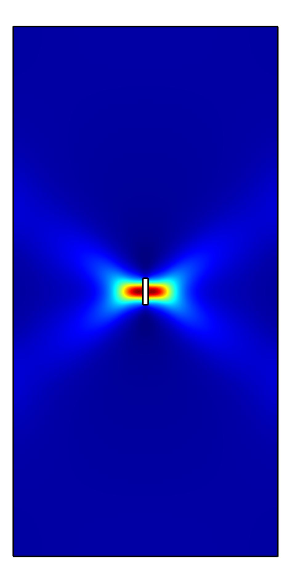
(a) $u=0.1976$ mm

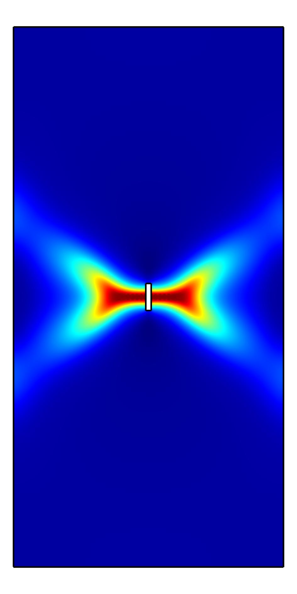
(b) $u=0.1980$ mm

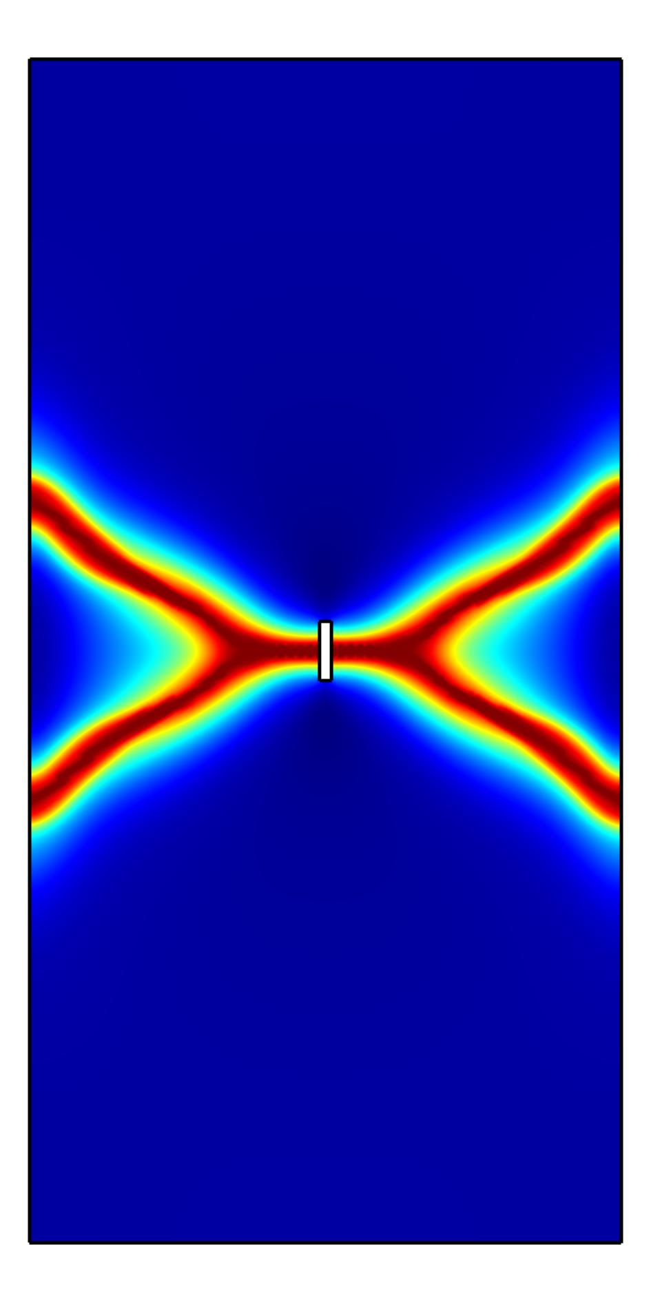
(c) $u=0.1981$ mm

Figure 14: Fracture patterns of a specimen with an inclined flaw of $\alpha=90^{\circ}$

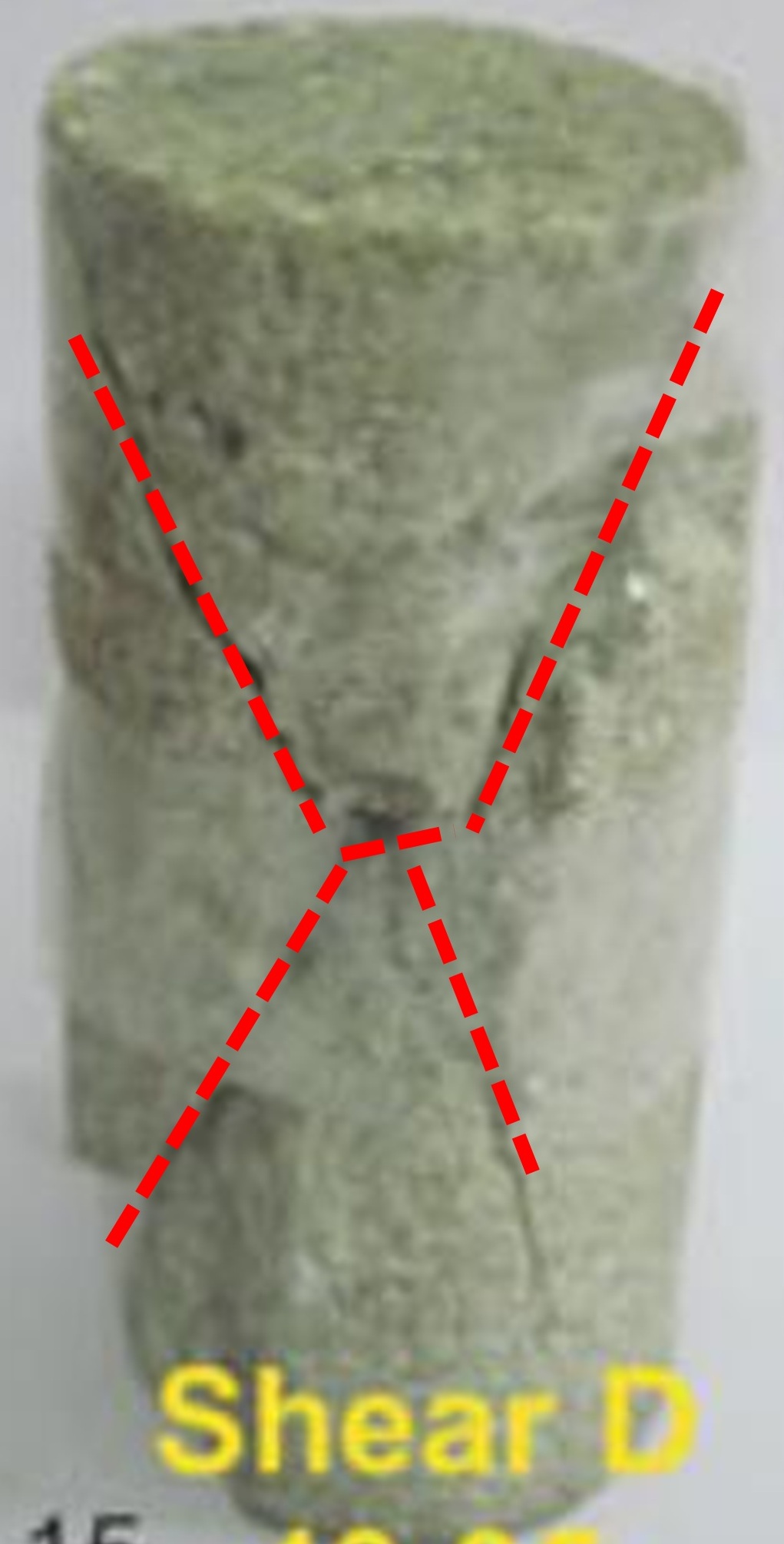
Figure 15: Experimental observation of the double shear fractures in rocks [8]

The load-displacement curves of the specimen with an inclined flaw under different angles are shown in Fig. 16. As observed, the maximum load that the specimen can sustain increases with the increase in the inclination angle under the compressive-shear mode. Moreover, the maximum displacement of the specimen increases because the factual load-bearing area increases as the angle of inclination increases. The influence of the energy release rate $G_{c}$ and length scale parameter $l_{0}$ on the fracture propagation are also tested. Herein, we set $G_{c}$ = 100, 200, 300, and 400 N/m and $l_{0}$ = 0.5 mm and 1 mm while the other base parameters are fixed. It is found that the fracture patterns are not affected by the energy release rate and length scale. However, a larger length scale $l_{0}$ produces a larger fracture width, as shown in Fig. 17. In addition, the load-displacement curves under different $G_{c}$ and $l_{0}$ are shown in Figs. 18 and 19. As expected, the peak load of the specimen increases with an increasing $G_{c}$ but a decreasing $l_{0}$. Figure 19 indicates that the proposed PFM is sensitive to the length scale parameter and in the future the new driving force proposed in this work can be coupled to the length-scale insensitive phase field framework proposed by Mandal et al. [70]; Wu and Nguyen [71] to overcome this kind of sensitivity.

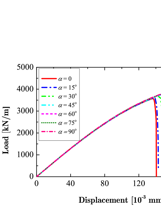
Figure 16: Load-displacement curves of the specimen with an inclined flaw under different angles

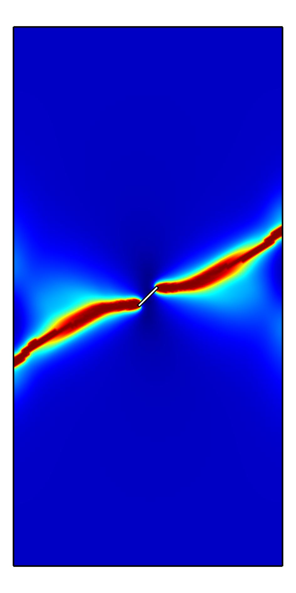
(a) $l_{0}=0.5$ mm

(b) $l_{0}=1$ mm

Figure 17: Fracture patterns of a specimen with an inclined flaw ($\alpha=45^{\circ}$) under different $l_{0}$

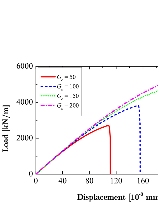
Figure 18: Load-displacement curves of the specimen with an inclined flaw under different $G_{c}$

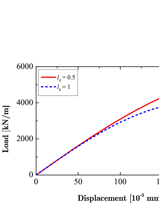
Figure 19: Load-displacement curves of the specimen with an inclined flaw under different $l_{0}$

Finally, we test the influence of the cohesion $c$, internal friction angle $\varphi$, and eccentricity $e$ on the compressive-shear fracture pattern. We adopt $c=$ 100, 500, 1000 and 5000 kPa, $\varphi=5^{\circ}$, $10^{\circ}$, $15^{\circ}$ and $20^{\circ}$, and $e$ = 0, 5 and 10 mm while keeping the other base parameters unchanged. The numerical results show that the fracture pattern is not affected by the cohesion and internal friction angle. In addition, the load-displacement curves of the specimen under different $c$ and $\varphi$ are presented in Figs. 20 and 21, respectively. As observed, the peak loads of the specimen increase with the increase in cohesion $c$ and internal friction angle $\varphi$, which accurately reflects the compressive-shear nature in rock fractures and corresponds to those experimental observations in rock tests.

Figure 22 shows the fracture patterns of the specimen under different eccentricity $e$. With the increase in the eccentricity $e$, the compressive-shear fracture is found to propagate at a decreasing inclination angle to the horizontal direction. However, the load-displacement curves in Fig. 23 indicates an ignorable decrease in the peak load of the specimen because the factual load-bearing area under compression is almost unchanged under different $e$. In summary, the proposed phase field method can model well the compressive-shear fractures in the rock-like specimen with an inclined flaw, and can reflect the increase in the load-bearing capacity under compression as the intrinsic cohesion and internal friction angle of the materials increase.

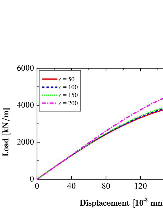
Figure 20: Load-displacement curves of the specimen with an inclined flaw under different $c$

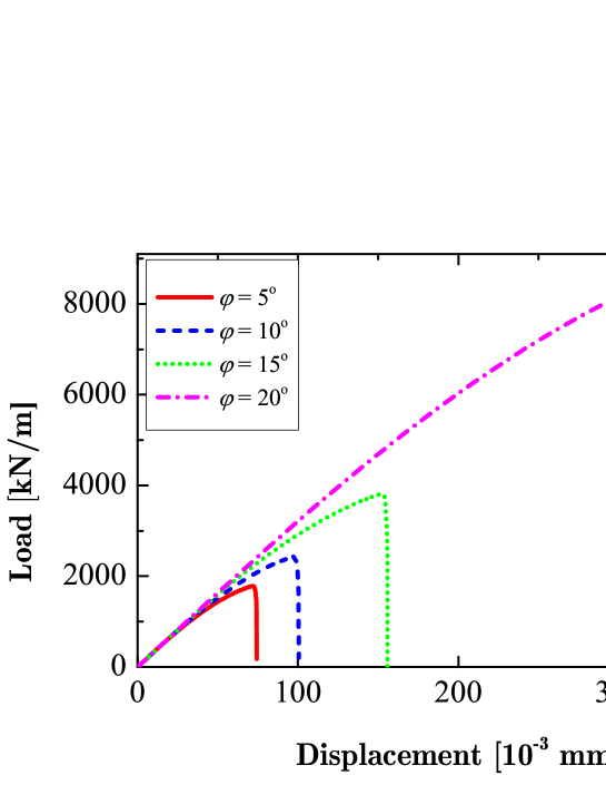
Figure 21: Load-displacement curves of the specimen with an inclined flaw under different $\varphi$

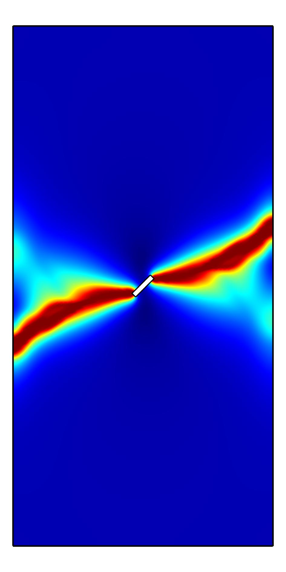
(a) $e=0$

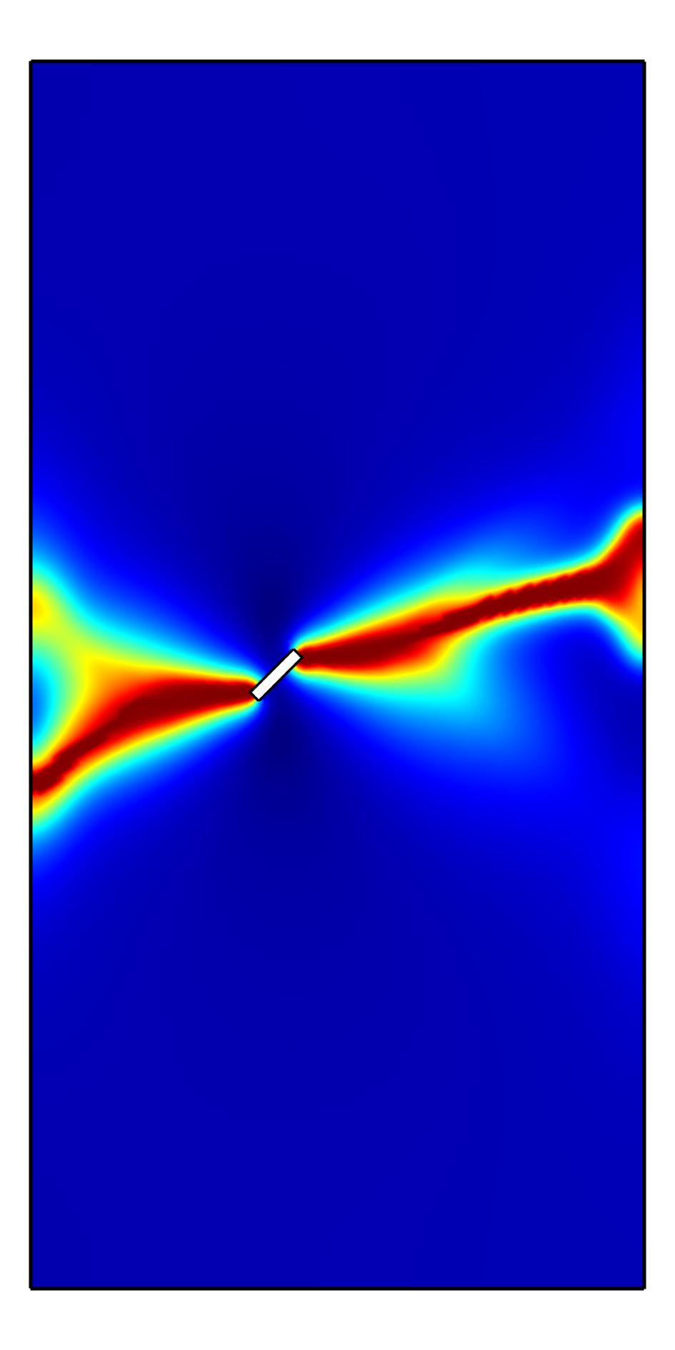
(b) $e=5$ mm

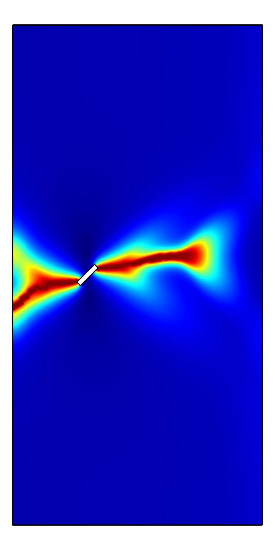
(c) $e=10$ mm

Figure 22: Fracture patterns of a specimen with an inclined flaw ($\alpha=45^{\circ}$) under different $e$

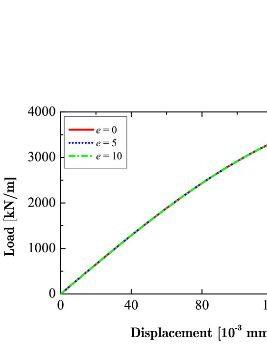
Figure 23: Load-displacement curves of the specimen with an inclined flaw under different $e$

5.3 Uniaxial compression of a specimen with two parallel inclined flaws

In this final example, we test the compressive-shear fractures in a rock-like specimen with two parallel inclined flaws. Uniaxial compression is applied on the upper end of the specimen along with the geometry of the problem shown in Fig. 24. The inclination angle, length, and width of the flaws are $30^{\circ}$, 7.5 mm, and 1 mm, respectively. Moreover, we set two types of flaw arrangement in Fig. 24, namely, the coplanar (Type A) and non-coplanar (Type B) pre-existing flaws. These parameters are used for the phase field simulations: Young’s modulus $E$ = 60 GPa, Poisson’s ratio $\nu$ = 0.3, critical energy release rate $G_{c}$ = 100 N/m, length scale parameter $l_{0}$ = 1 mm, $k=1\times 10^{-9}$, cohesion $c$ = 100 kPa, and internal friction angle $\varphi=15^{\circ}$. The specimen with two flaws are then discretized using triangular elements with the maximum element size $h$ = 0.5 mm. The simulation is proceeded under displacement control and we use a displacement increment $\Delta u=1\times 10^{-4}$ mm in this example.

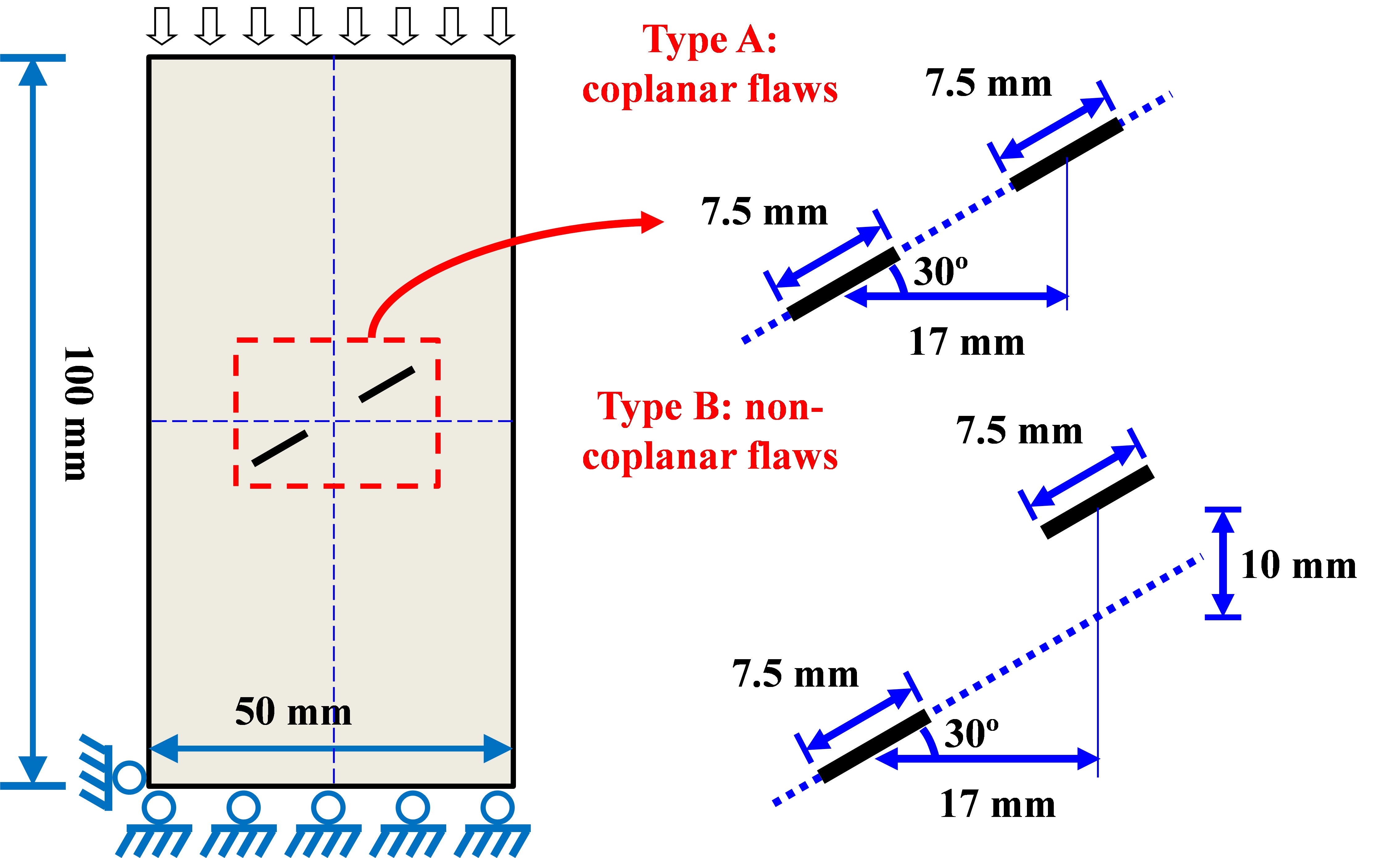
Figure 24: Geometry and boundary conditions of a rectangular specimen with two parallel inclined flaws subjected to uniaxial compression

Figure 25 shows the compressive-shear fracture propagation in the specimen with two coplanar pre-existing flaws (Type A). With the increase in the compressive loads, shear zones occur around the tips of the inclined flaws and the fractures initiate at $u=0.1178$ mm. When $u=0.1184$ mm, the fractures from the two inclined flaws coalesce. Fractures from the two pre-existing flaws reach the left and right boundaries of the specimen at $u=0.1200$ mm and quasi-coplanar fractures can be observed in Fig. 25c. Figure 26 shows the compressive-shear fracture propagation in the specimen with two non-coplanar pre-existing flaws (Type B). The fracture patterns are similar to those in Fig. 25. Fractures initiate at $u=0.1244$ mm while the fractures from the two inclined flaws coalesce and reach the left and right boundaries of the specimen at $u=0.1258$ mm. However, the S-shaped coalescence between the two pre-existing flaws is non-coplanar, which is different from the observations for the two coplanar flaws in Fig. 26. In addition, the load-displacement curves of the specimens with two parallel inclined flaws are shown in Fig. 27. The non-coplanar flaws are shown to have a larger peak load than the coplanar flaws because of the relatively large factual load-bearing area.

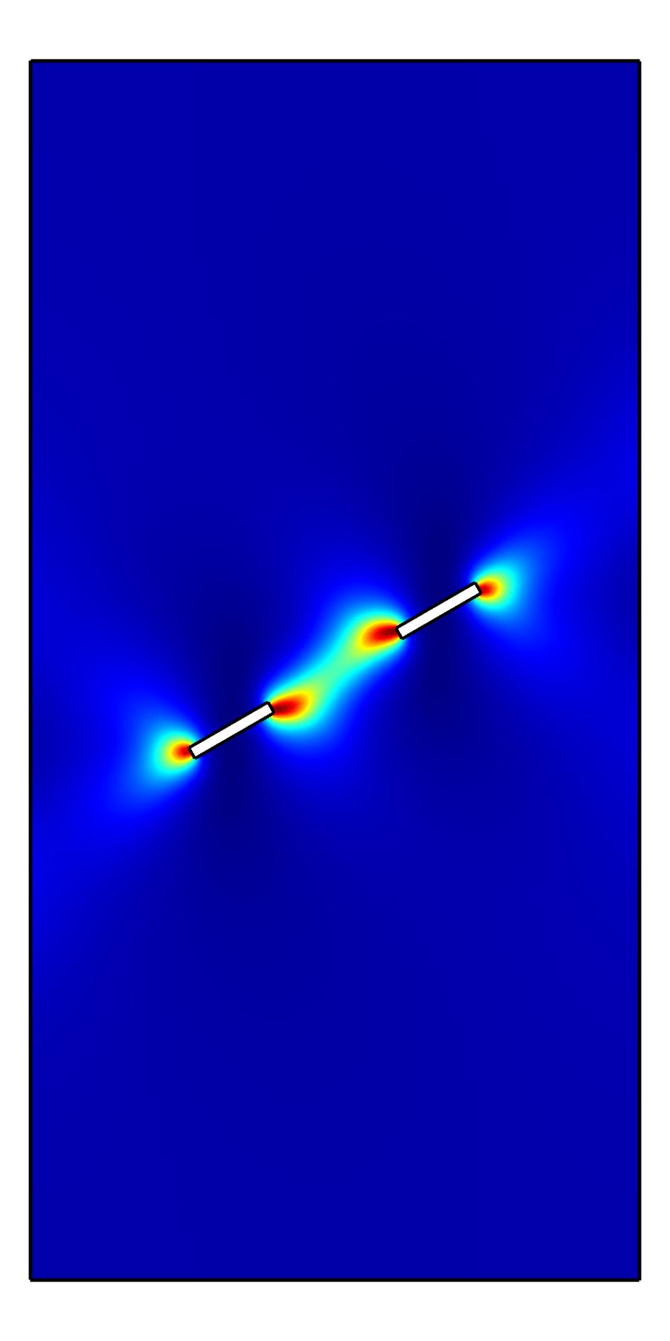
(a) $u=0.1178$ mm

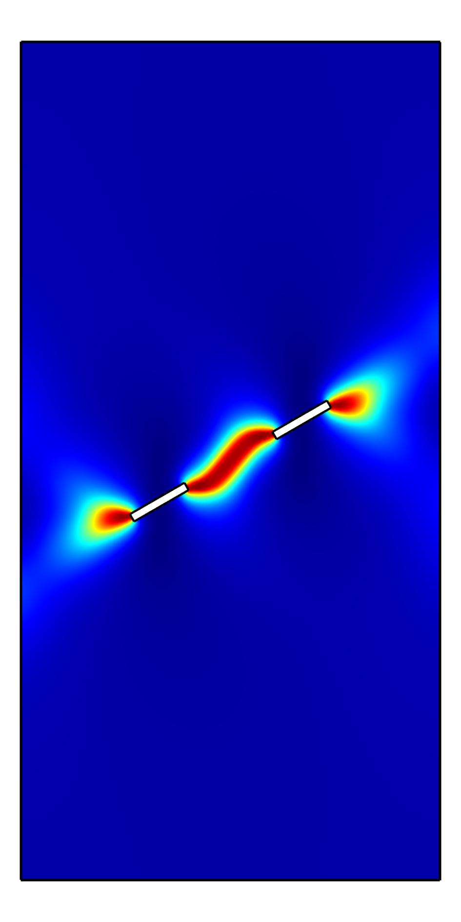
(b) $u=0.1184$ mm

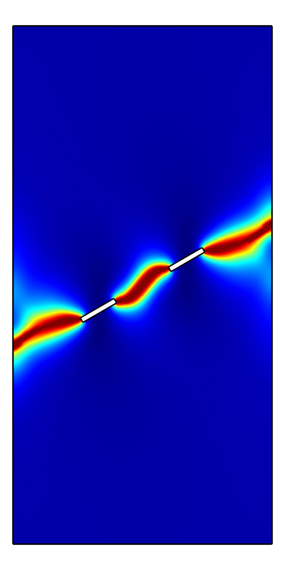
(c) $u=0.1200$ mm

Figure 25: Fracture patterns of a specimen with two parallel inclined flaws (coplanar flaws)

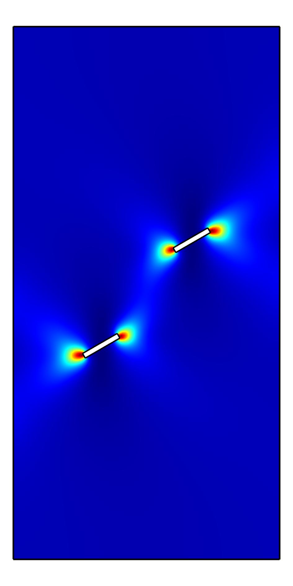
(a) $u=0.1244$ mm

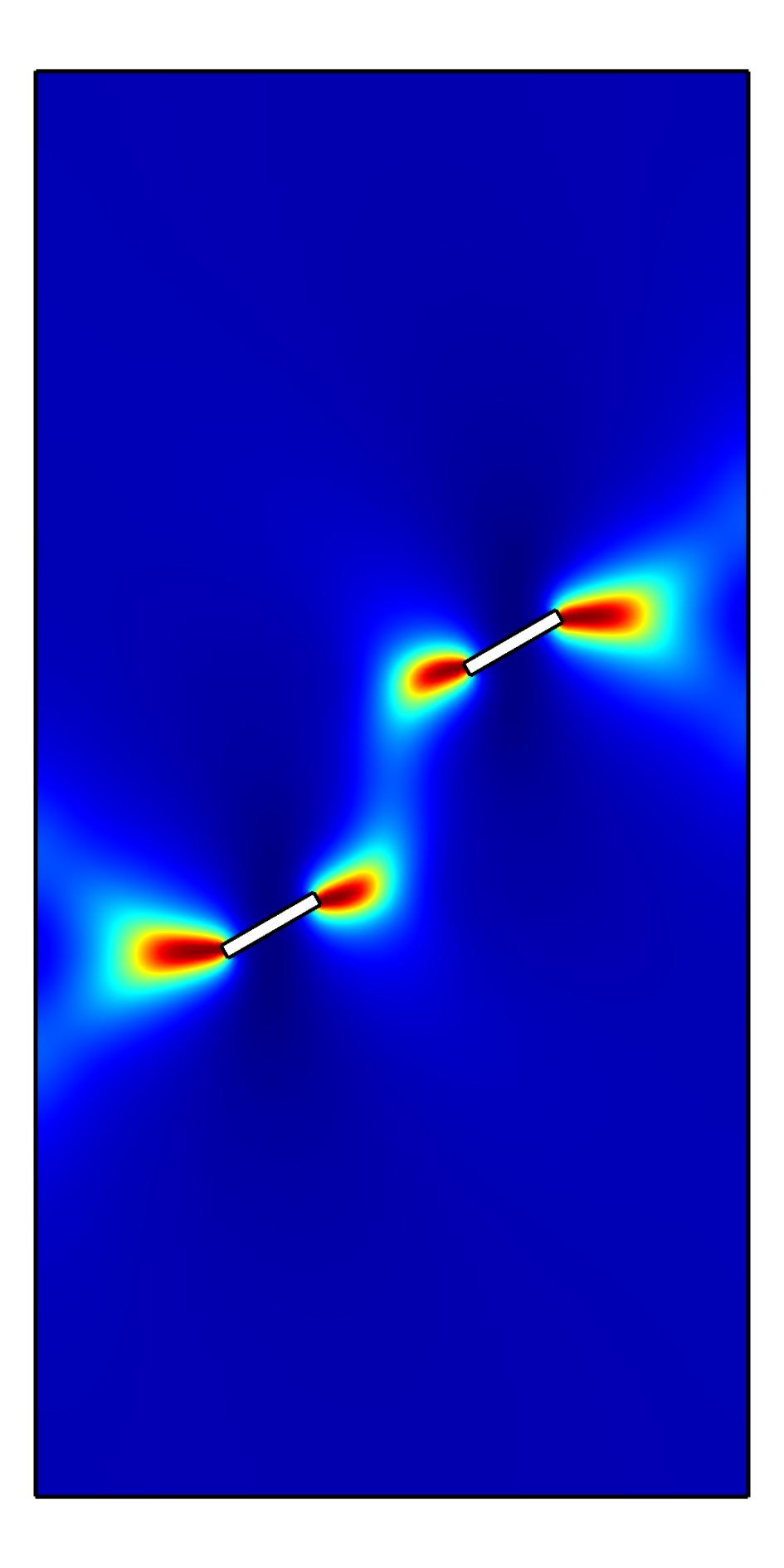
(b) $u=0.1256$ mm

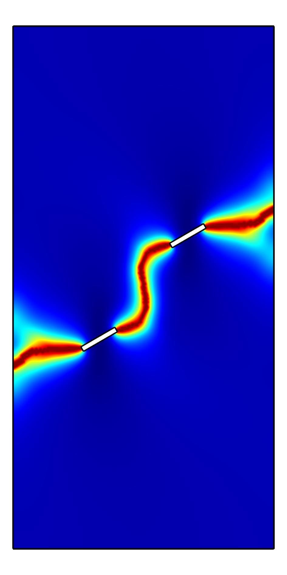
(c) $u=0.1258$ mm

Figure 26: Fracture patterns of a specimen with two parallel inclined flaws (non-coplanar flaws)

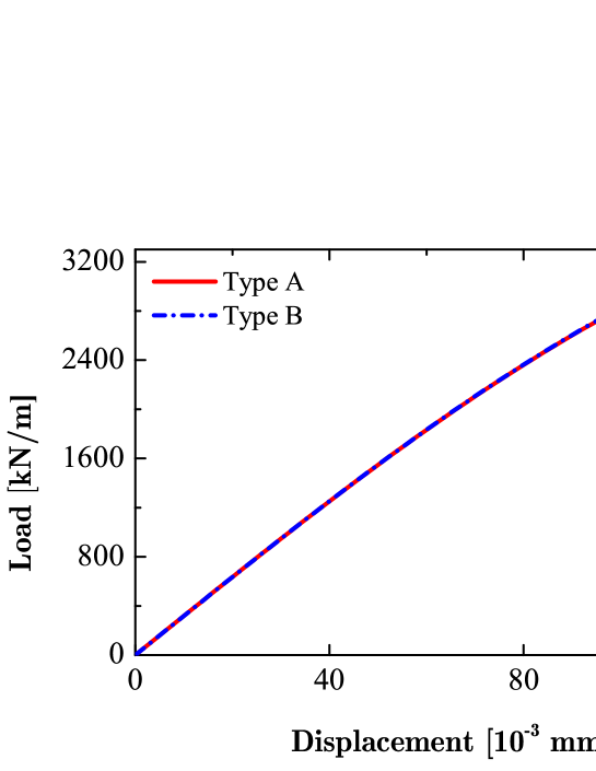
Figure 27: Load-displacement curves of the specimen with two parallel inclined flaws

Sagong and Bobet [5] performed compression tests on rock-like specimens with multiple inclined pre-existing flaws and summarized the patterns of fracture coalescence from the experimental observations. Among the nine patterns, two shear types, namely Types I and II are shown in Fig. 28. Note that the wing cracks (tensile fractures) are suppressed in Fig. 28 because this study focuses on the compressive-shear fractures and we don’t introduce and discuss any tensile fractures. Therefore, the compressive-shear fracture patterns obtained by using the proposed phase field method are in line with the experimental observations, validating the capability of the proposed model in predicting complex compressive-shear fractures in rock-like materials.

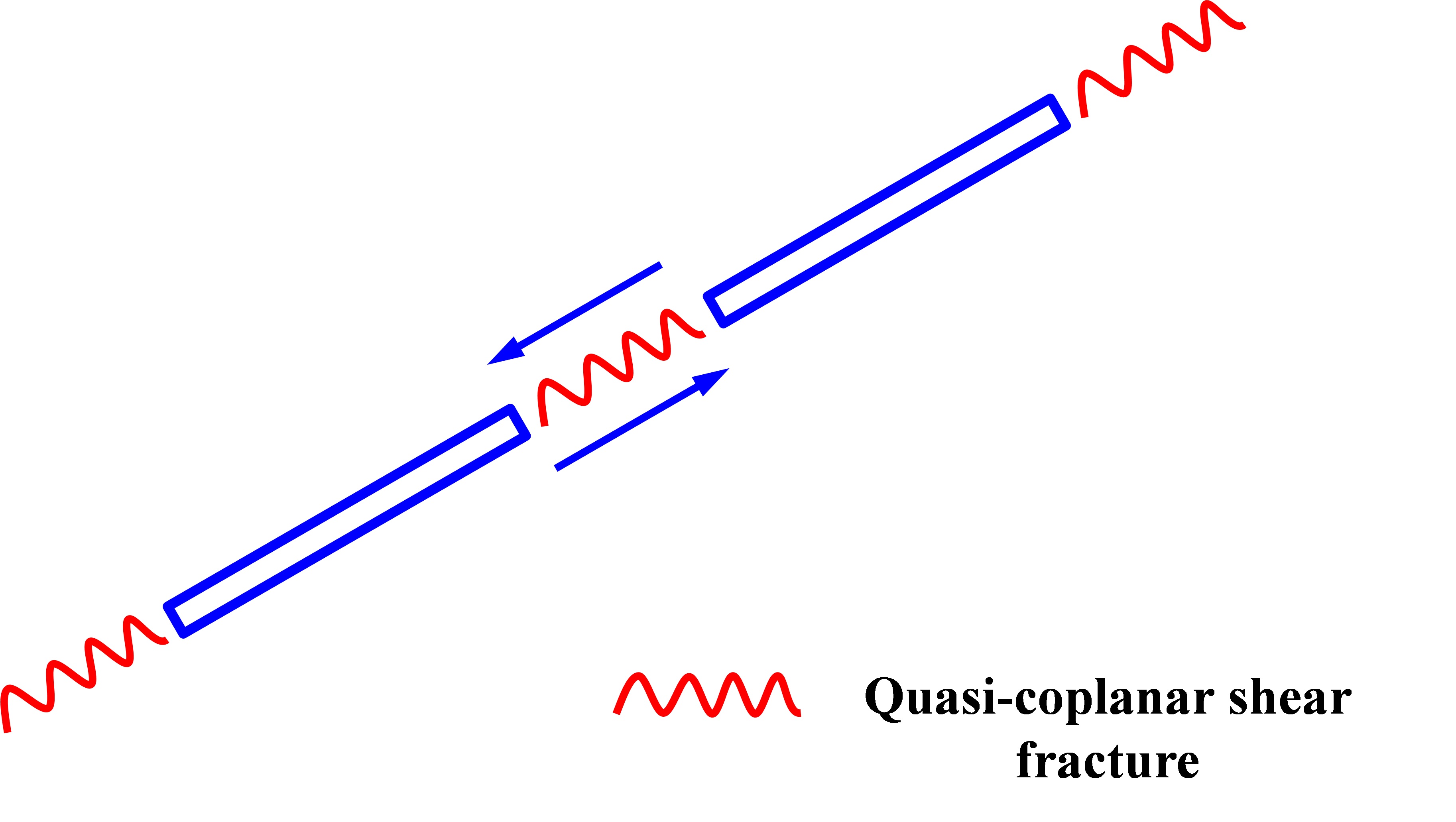
(a) Type I

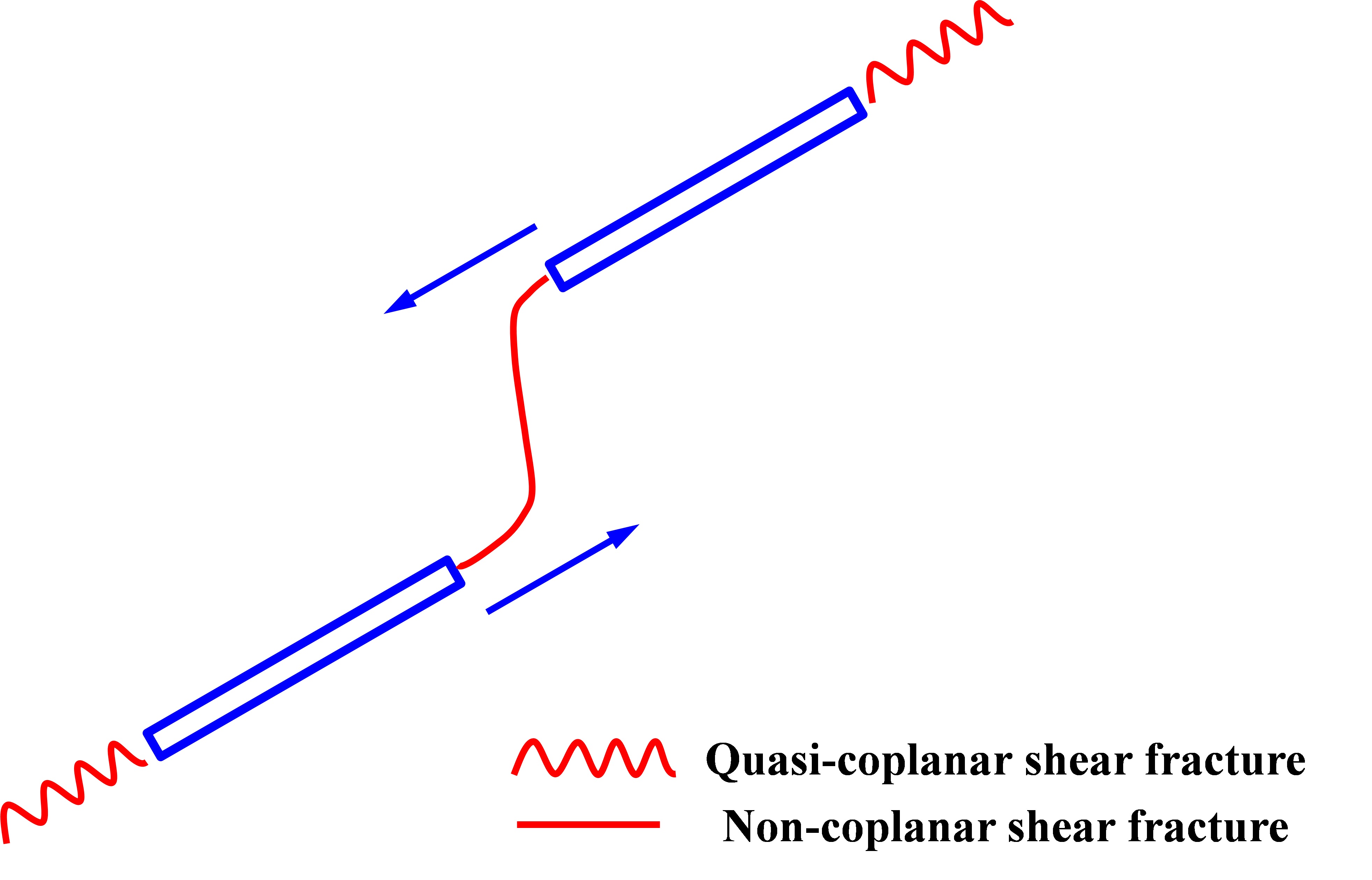
(b) Type II

Figure 28: Experimental observations of coalescence of two parallel inclined flaws [5]

6 Conclusions

A new phase field model is proposed for simulating brittle compressive-shear fractures in rock-like materials. By using the strain spectral decomposition and with emphasis on the compressive parts of the strain, a new driving force is re-constructed and applied in the evolution equation of phase field. The new driving force can also account for the influence of cohesion and internal friction angle on fracture propagation; this effect cannot be considered in other PFMs. We construct a hybrid formulation for the phase field modeling and implement the proposed model in COMSOL within the framework of conventional finite element method. We then simulate the brittle compressive-shear fractures in rock-like specimens subjected to uniaxial compression. These specimens include intact specimens and specimens with a single inclined flaw or two parallel inclined flaws. The presented numerical results are in good agreement with previous experimental results, validating the feasibility and practicability of the proposed phase field model for simulating brittle compressive-shear fractures.

All the presented numerical examples show that the initiation, propagation, coalescence, and branching of compressive-shear fractures are autonomous without any external fracture criteria or setting a propagation path in advance. This highlights the advantages of the proposed phase field method over other numerical methods in modeling complex compressive-shear fractures in rock-like materials. In addition, because the tensile part of the strain is suppressed in the proposed model, tensile fractures and fractures under tension-shear mode are not included in this new model. In this sense, an improved phase field model that combines the presented new driving force and those previously used will be attractive in the future, especially for the mixed-mode fractures commonly seen in rocks.

References

- Zhou et al. [2015a] S.-W. Zhou, C.-C. Xia, S.-G. Du, P.-Y. Zhang, Y. Zhou, An analytical solution for mechanical responses induced by temperature and air pressure in a lined rock cavern for underground compressed air energy storage, Rock Mechanics and Rock Engineering 48 (2) (2015a) 749–770.
- Zhou et al. [2017a] S.-W. Zhou, C.-C. Xia, H.-B. Zhao, S.-H. Mei, Y. Zhou, Numerical simulation for the coupled thermo-mechanical performance of a lined rock cavern for underground compressed air energy storage, Journal of Geophysics and Engineering 14 (6) (2017a) 1382.
- Zhou et al. [2018a] S. Zhou, X. Zhuang, H. Zhu, T. Rabczuk, Phase field modelling of crack propagation, branching and coalescence in rocks, Theoretical and Applied Fracture Mechanics 96 (2018a) 174–192.
- Lajtai [1974] E. Lajtai, Brittle fracture in compression, International Journal of Fracture 10 (4) (1974) 525–536.
- Sagong and Bobet [2002] M. Sagong, A. Bobet, Coalescence of multiple flaws in a rock-model material in uniaxial compression, International Journal of Rock Mechanics and Mining Sciences 39 (2) (2002) 229–241.
- Wong and Einstein [2009] L. Wong, H. Einstein, Systematic evaluation of cracking behavior in specimens containing single flaws under uniaxial compression, International Journal of Rock Mechanics and Mining Sciences 46 (2) (2009) 239–249.
- Yang and Jing [2011] S.-Q. Yang, H.-W. Jing, Strength failure and crack coalescence behavior of brittle sandstone samples containing a single fissure under uniaxial compression, International Journal of Fracture 168 (2) (2011) 227–250.
- Basu et al. [2013] A. Basu, D. Mishra, K. Roychowdhury, Rock failure modes under uniaxial compression, Brazilian, and point load tests, Bulletin of Engineering Geology and the environment 72 (3-4) (2013) 457–475.
- Xia et al. [2015] C.-C. Xia, S.-W. Zhou, P.-Y. Zhang, Y.-S. Hu, Y. Zhou, Strength criterion for rocks subjected to cyclic stress and temperature variations, Journal of Geophysics and Engineering 12 (5) (2015) 753.
- Zhou et al. [2015b] S. Zhou, C. Xia, Y. Hu, Y. Zhou, P. Zhang, Damage modeling of basaltic rock subjected to cyclic temperature and uniaxial stress, International Journal of Rock Mechanics and Mining Sciences 77 (2015b) 163–173.
- Zhou et al. [2017b] S.-W. Zhou, C.-C. Xia, H.-B. Zhao, S.-H. Mei, Y. Zhou, Statistical damage constitutive model for rocks subjected to cyclic stress and cyclic temperature, Acta Geophysica 65 (5) (2017b) 893–906.
- Ingraffea and Saouma [1985] A. Ingraffea, V. Saouma, Numerical modelling of discrete crack propagation in reinforced and plain concrete, Fracture Mechanics of concrete (1985) 171–225.
- Moës and Belytschko [2002] N. Moës, T. Belytschko, Extended finite element method for cohesive crack growth, Engineering fracture mechanics 69 (7) (2002) 813–833.
- Chen et al. [2012] L. Chen, T. Rabczuk, S. P. A. Bordas, G. Liu, K. Zeng, P. Kerfriden, Extended finite element method with edge-based strain smoothing (ESm-XFEM) for linear elastic crack growth, Computer Methods in Applied Mechanics and Engineering 209 (2012) 250–265.
- Fu et al. [2013] Z.-J. Fu, W. Chen, H.-T. Yang, Boundary particle method for Laplace transformed time fractional diffusion equations, Journal of Computational Physics 235 (2013) 52–66.
- Fu et al. [2019] Z.-J. Fu, S. Reutskiy, H.-G. Sun, J. Ma, M. A. Khan, A robust kernel-based solver for variable-order time fractional PDEs under 2D/3D irregular domains, Applied Mathematics Letters 94 (2019) 105–111.
- Xi et al. [2019] Q. Xi, Z.-J. Fu, T. Rabczuk, An efficient boundary collocation scheme for transient thermal analysis in large-size-ratio functionally graded materials under heat source load, Computational Mechanics (2019) 1–15.
- Fries and Belytschko [2010] T.-P. Fries, T. Belytschko, The extended/generalized finite element method: an overview of the method and its applications, International Journal for Numerical Methods in Engineering 84 (3) (2010) 253–304.
- Chau-Dinh et al. [2012] T. Chau-Dinh, G. Zi, P.-S. Lee, T. Rabczuk, J.-H. Song, Phantom-node method for shell models with arbitrary cracks, Computers & Structures 92 (2012) 242–256.
- Rabczuk et al. [2008] T. Rabczuk, G. Zi, A. Gerstenberger, W. A. Wall, A new crack tip element for the phantom-node method with arbitrary cohesive cracks, International Journal for Numerical Methods in Engineering 75 (5) (2008) 577–599.
- Zhang et al. [2017a] X. Zhang, S. W. Sloan, C. Vignes, D. Sheng, A modification of the phase-field model for mixed mode crack propagation in rock-like materials, Computer Methods in Applied Mechanics and Engineering 322 (2017a) 123–136.
- Peerlings et al. [1996] R. Peerlings, R. De Borst, W. Brekelmans, J. De Vree, I. Spee, Some observations on localisation in non-local and gradient damage models, European Journal of Mechanics A: Solids 15 (6) (1996) 937–953.
- Areias et al. [2016a] P. Areias, M. Msekh, T. Rabczuk, Damage and fracture algorithm using the screened Poisson equation and local remeshing, Engineering Fracture Mechanics 158 (2016a) 116–143.
- Areias et al. [2016b] P. Areias, T. Rabczuk, J. C. de Sá, A novel two-stage discrete crack method based on the screened Poisson equation and local mesh refinement, Computational Mechanics 58 (6) (2016b) 1003–1018.
- Miehe et al. [2010a] C. Miehe, F. Welschinger, M. Hofacker, Thermodynamically consistent phase-field models of fracture: Variational principles and multi-field FE implementations, International Journal for Numerical Methods in Engineering 83 (10) (2010a) 1273–1311.
- Miehe et al. [2010b] C. Miehe, M. Hofacker, F. Welschinger, A phase field model for rate-independent crack propagation: Robust algorithmic implementation based on operator splits, Computer Methods in Applied Mechanics and Engineering 199 (45) (2010b) 2765–2778.
- Borden et al. [2012] M. J. Borden, C. V. Verhoosel, M. A. Scott, T. J. Hughes, C. M. Landis, A phase-field description of dynamic brittle fracture, Computer Methods in Applied Mechanics and Engineering 217 (2012) 77–95.
- Bourdin et al. [2008] B. Bourdin, G. A. Francfort, J.-J. Marigo, The variational approach to fracture, Journal of elasticity 91 (1) (2008) 5–148.
- Hesch and Weinberg [2014] C. Hesch, K. Weinberg, Thermodynamically consistent algorithms for a finite-deformation phase-field approach to fracture, International Journal for Numerical Methods in Engineering 99 (12) (2014) 906–924.
- Zhou et al. [2018b] S. Zhou, T. Rabczuk, X. Zhuang, Phase field modeling of quasi-static and dynamic crack propagation: COMSOL implementation and case studies, Advances in Engineering Software 122 (2018b) 31–49.
- Zhou et al. [2018c] S. Zhou, X. Zhuang, T. Rabczuk, A phase-field modeling approach of fracture propagation in poroelastic media, Engineering Geology 240 (2018c) 189–203.
- Zhou and Xia [2018] S.-W. Zhou, C.-C. Xia, Propagation and coalescence of quasi-static cracks in Brazilian disks: an insight from a phase field model, Acta Geotechnica (2018) 1–20.
- Zhou and Zhuang [2018] S. Zhou, X. Zhuang, Adaptive phase field simulation of quasi-static crack propagation in rocks, Underground Space 3 (3) (2018) 190 – 205.
- Nguyen and Wu [2018] V. P. Nguyen, J.-Y. Wu, Modeling dynamic fracture of solids with a phase-field regularized cohesive zone model, Computer Methods in Applied Mechanics and Engineering 340 (2018) 1000–1022.
- Miehe et al. [2014] C. Miehe, F. Welschinger, F. Aldakheel, Variational gradient plasticity at finite strains. Part II: Local–global updates and mixed finite elements for additive plasticity in the logarithmic strain space, Computer Methods in Applied Mechanics and Engineering 268 (2014) 704–734.
- Ambati and De Lorenzis [2016] M. Ambati, L. De Lorenzis, Phase-field modeling of brittle and ductile fracture in shells with isogeometric NURBS-based solid-shell elements, Computer Methods in Applied Mechanics and Engineering 312 (2016) 351–373.
- Borden et al. [2016] M. J. Borden, T. J. Hughes, C. M. Landis, A. Anvari, I. J. Lee, A phase-field formulation for fracture in ductile materials: Finite deformation balance law derivation, plastic degradation, and stress triaxiality effects, Computer Methods in Applied Mechanics and Engineering 312 (2016) 130–166.
- Shanthraj et al. [2016] P. Shanthraj, L. Sharma, B. Svendsen, F. Roters, D. Raabe, A phase field model for damage in elasto-viscoplastic materials, Computer Methods in Applied Mechanics and Engineering 312 (2016) 167–185.
- Verhoosel and de Borst [2013] C. V. Verhoosel, R. de Borst, A phase-field model for cohesive fracture, International Journal for numerical methods in Engineering 96 (1) (2013) 43–62.
- Vignollet et al. [2014] J. Vignollet, S. May, R. De Borst, C. V. Verhoosel, Phase-field models for brittle and cohesive fracture, Meccanica 49 (11) (2014) 2587–2601.
- Natarajan et al. [2019a] S. Natarajan, R. K. Annabattula, et al., Modeling crack propagation in variable stiffness composite laminates using the phase field method, Composite Structures 209 (2019a) 424–433.
- Natarajan et al. [2019b] S. Natarajan, R. K. Annabattula, E. Martínez-Pañeda, et al., Phase field modelling of crack propagation in functionally graded materials, Composites Part B: Engineering 169 (2019b) 239–248.
- Miehe et al. [2015] C. Miehe, M. Hofacker, L.-M. Schänzel, F. Aldakheel, Phase field modeling of fracture in multi-physics problems. Part II. Coupled brittle-to-ductile failure criteria and crack propagation in thermo-elastic–plastic solids, Computer Methods in Applied Mechanics and Engineering 294 (2015) 486–522.
- Lee et al. [2016] S. Lee, M. F. Wheeler, T. Wick, Pressure and fluid-driven fracture propagation in porous media using an adaptive finite element phase field model, Computer Methods in Applied Mechanics and Engineering 305 (2016) 111–132.
- Miehe and Mauthe [2016] C. Miehe, S. Mauthe, Phase field modeling of fracture in multi-physics problems. Part III. Crack driving forces in hydro-poro-elasticity and hydraulic fracturing of fluid-saturated porous media, Computer Methods in Applied Mechanics and Engineering 304 (2016) 619–655.
- Ehlers and Luo [2017] W. Ehlers, C. Luo, A phase-field approach embedded in the Theory of Porous Media for the description of dynamic hydraulic fracturing, Computer Methods in Applied Mechanics and Engineering 315 (2017) 348–368.
- Li and Zhou [2019] K. Li, S. Zhou, Numerical investigation of multizone hydraulic fracture propagation in porous media: new insights from a phase field method, Journal of Natural Gas Science and Engineering 66 (2019) 42–59.
- Zhou et al. [2019] S. Zhou, X. Zhuang, T. Rabczuk, Phase-field modeling of fluid-driven dynamic cracking in porous media, Computer Methods in Applied Mechanics and Engineering 350 (2019) 169–198.
- HIRSHIKESH [2019] R. K. A. HIRSHIKESH, Sundararajan NATARAJAN, A FEniCS implementation of the phase field method for quasi-static brittle fracture, Frontiers of Structural and Civil Engineering 13 (2) (2019) 380–396.
- Zhou [2018] S. Zhou, Fracture Propagation in Brazilian Discs with Multiple Pre-existing Notches by Using a Phase Field Method, Periodica Polytechnica Civil Engineering 62 (3) (2018) 700–708.
- Choo and Sun [2018] J. Choo, W. Sun, Coupled phase-field and plasticity modeling of geological materials: From brittle fracture to ductile flow, Computer Methods in Applied Mechanics and Engineering 330 (2018) 1–32.
- Bryant and Sun [2018] E. C. Bryant, W. Sun, A mixed-mode phase field fracture model in anisotropic rocks with consistent kinematics, Computer Methods in Applied Mechanics and Engineering 342 (2018) 561–584.
- Ambati et al. [2015] M. Ambati, T. Gerasimov, L. De Lorenzis, A review on phase-field models of brittle fracture and a new fast hybrid formulation, Computational Mechanics 55 (2) (2015) 383–405.
- Aranson et al. [2000] I. Aranson, V. Kalatsky, V. Vinokur, Continuum field description of crack propagation, Physical review letters 85 (1) (2000) 118.
- Karma et al. [2001] A. Karma, D. A. Kessler, H. Levine, Phase-field model of mode III dynamic fracture, Physical Review Letters 87 (4) (2001) 045501.
- Henry and Levine [2004] H. Henry, H. Levine, Dynamic instabilities of fracture under biaxial strain using a phase field model, Physical review letters 93 (10) (2004) 105504.
- Bourdin et al. [2000] B. Bourdin, G. A. Francfort, J.-J. Marigo, Numerical experiments in revisited brittle fracture, Journal of the Mechanics and Physics of Solids 48 (4) (2000) 797–826.
- Wu [2017] J.-Y. Wu, A unified phase-field theory for the mechanics of damage and quasi-brittle failure, Journal of the Mechanics and Physics of Solids 103 (2017) 72–99.
- Zhou et al. [2018d] S. Zhou, C. Xia, Y. Zhou, A theoretical approach to quantify the effect of random cracks on rock deformation in uniaxial compression, Journal of Geophysics and Engineering 15 (3) (2018d) 627.
- Amor et al. [2009] H. Amor, J.-J. Marigo, C. Maurini, Regularized formulation of the variational brittle fracture with unilateral contact: Numerical experiments, Journal of the Mechanics and Physics of Solids 57 (8) (2009) 1209–1229.
- Li et al. [2012] X. Li, W.-G. Cao, Y.-H. Su, A statistical damage constitutive model for softening behavior of rocks, Engineering Geology 143 (2012) 1–17.
- Li et al. [2017] Z. Li, Q.-h. Zhu, B.-l. Tian, T.-f. Sun, D.-w. Yang, A damage model for hard rock under stress-induced failure mode, in: Advanced Engineering and Technology III: Proceedings of the 3rd Annual Congress on Advanced Engineering and Technology (CAET 2016), Hong Kong, 22-23 October 2016, CRC Press, 87, 2017.
- Liu et al. [2016] G. Liu, Q. Li, M. A. Msekh, Z. Zuo, Abaqus implementation of monolithic and staggered schemes for quasi-static and dynamic fracture phase-field model, Computational Materials Science 121 (2016) 35–47.
- Kuhn and Müller [2008] C. Kuhn, R. Müller, A phase field model for fracture, PAMM 8 (1) (2008) 10223–10224.
- Bourdin et al. [2012] B. Bourdin, C. P. Chukwudozie, K. Yoshioka, et al., A variational approach to the numerical simulation of hydraulic fracturing, in: SPE Annual Technical Conference and Exhibition, Society of Petroleum Engineers, 2012.
- Zhou et al. [2018e] S. Zhou, C. Xia, Y. Zhou, Long-term stability of a lined rock cavern for compressed air energy storage: thermo-mechanical damage modeling, European Journal of Environmental and Civil Engineering (2018e) 1–24.
- Zhang et al. [2017b] X. Zhang, C. Vignes, S. W. Sloan, D. Sheng, Numerical evaluation of the phase-field model for brittle fracture with emphasis on the length scale, Computational Mechanics 59 (5) (2017b) 737–752.
- Ingraffea and Heuze [1980] A. R. Ingraffea, F. E. Heuze, Finite element models for rock fracture mechanics, International Journal for Numerical and Analytical Methods in Geomechanics 4 (1) (1980) 25–43.
- Zhuang et al. [2014] X. Zhuang, J. Chun, H. Zhu, A comparative study on unfilled and filled crack propagation for rock-like brittle material, Theoretical and Applied Fracture Mechanics 72 (2014) 110–120.
- Mandal et al. [2019] T. K. Mandal, V. P. Nguyen, A. Heidarpour, Phase field and gradient enhanced damage models for quasi-brittle failure: A numerical comparative study, Engineering Fracture Mechanics 207 (2019) 48–67.
- Wu and Nguyen [2018] J.-Y. Wu, V. P. Nguyen, A length scale insensitive phase-field damage model for brittle fracture, Journal of the Mechanics and Physics of Solids 119 (2018) 20–42.