FrozenRecon: Pose-free 3D Scene Reconstruction with Frozen Depth Models

Abstract

3D scene reconstruction is a long-standing vision task. Existing approaches can be categorized into geometry-based and learning-based methods. The former leverages multi-view geometry but can face catastrophic failures due to the reliance on accurate pixel correspondence across views. The latter was proffered to mitigate these issues by learning 2D or 3D representation directly. However, without a large-scale video or 3D training data, it can hardly generalize to diverse real-world scenarios due to the presence of tens of millions or even billions of optimization parameters in the deep network.

Recently, robust monocular depth estimation models trained with large-scale datasets have been proven to possess weak 3D geometry prior, but they are insufficient for reconstruction due to the unknown camera parameters, the affine-invariant property, and inter-frame inconsistency. Here, we propose a novel test-time optimization approach that can transfer the robustness of affine-invariant depth models such as LeReS to challenging diverse scenes while ensuring inter-frame consistency, with only dozens of parameters to optimize per video frame. Specifically, our approach involves freezing the pre-trained affine-invariant depth model’s depth predictions, rectifying them by optimizing the unknown scale-shift values with a geometric consistency alignment module, and employing the resulting scale-consistent depth maps to robustly obtain camera poses and achieve dense scene reconstruction, even in low-texture regions. Experiments show that our method achieves state-of-the-art cross-dataset reconstruction on five zero-shot testing datasets. Project webpage is at: https://aim-uofa.github.io/FrozenRecon/

1 Introduction

Dense 3D reconstruction is a fundamental vision task, which has a wide range of applications in autonomous driving [8], virtual$/$augmented reality [5, 40], robot navigation, medical-CAD modeling [33], etc. Existing geometry-based methods and learning-based methods have achieved impressive performance. Despite progress, we observe failure cases in certain real-world scenarios, such as incomplete or noisy reconstruction of low-texture scenes, tracking failures for pose estimation, limited generalization to unseen scenes, etc. In this work, we aim to robustly and efficiently reconstruct diverse scenes on monocular videos, with the intrinsic camera parameters and poses jointly optimized at the same time.

Most 3D scene reconstruction algorithms can be categorized into learning-based [21, 31, 38] and geometry-based methods [46, 3, 4, 15, 41, 18, 16, 17]. The first group of methods typically rely on a strong neural network to learn the scene geometry, which often requires large-scale and high-quality data to optimize for millions or billions of learnable parameters. Such an expensive data requirement limits applications to various scenarios. Furthermore, some methods, such as SC-DepthV3 [32], optimize the depth and poses at the same time, for which the optimization can be challenging and may become stuck in trivial solutions, partly due to the large number of optimization parameters.

In contrast, geometry-based methods find feature correspondences across views to achieve dense 3D reconstruction. Thus, fewer$/$no training data are needed. The drawback is that these methods can easily fail on texture-less or low-texture scenes. Moreover, planar scenes and in-place rotations also lead to degeneration in camera pose optimization. Occlusion, lighting changes, and low-texture regions can make the dense matching intractable and thus lead to incomplete reconstructions. Seeking to mitigate these limitations, we propose to exploit a pre-trained, robust monocular depth model to obtain scene geometry priors, which can largely ease pose optimization and reconstruction.

Recently, foundation models [22, 1] trained with large-scale datasets can generalize to new datasets/tasks with few samples by optimizing for a small portion of parameters (so-called adaptors). Inspired by the success, we use a pre-trained monocular depth model of strong performance such as LeReS [44], and optimize for a very sparse set of parameters for quickly rectifying the depth maps on test videos, such that scale-consistent depth maps can be attained.

Models such as LeReS [44], MiDaS [24], and DPT [23] use millions of training images to train a robust monocular depth model, which generalizes well to diverse scenes. Unfortunately, the predicted depth maps of those models are affine-invariant, i.e., up to an unknown scale and shift compared against the ground-truth metric depth. As pointed out in [44], the unknown shift can cause significant distortion. Naively fusing pre-frame prediction is prone to cause reconstruction distortion and scale misalignment. Furthermore, the unknown intrinsic camera parameters and poses are another obstacle for multi-frame reconstruction. If we have access to accurate camera parameters, we can fine tune the pre-trained model to solve the above issues, as in [18].

Instead, we freeze the monocular depth model, and on the given videos, we optimize for the global scale value, the global shift value, a local scale map and a local shift map to rectify each predicted affine-invariant depth map. Intrinsic camera parameters and camera poses are also optimized at the same time. The number of parameters that need to be optimized online is only around 30 per frame. This is a sharp contrast compared with learning-based approaches, e.g., SC-DepthV3, where tens of millions of parameters are involved in optimization. The shift and scale parameters are optimized by supervising the photometric consistency and geometric consistency between selected keyframes. Due to the sparsity of optimization parameters and the robustness of the monocular depth model, our method works much better in terms of domain gap compared to existing deep learning methods for this task. At the same time, compared with traditional geometry-based 3D scene reconstruction methods, ours can be more robust to low-texture regions.

In order to validate the robustness of our system, we test on $5$ unseen datasets: NYU [29], ScanNet [9], 7-Scenes [28], TUM [30], and KITTI [13]. Experiments show that our pipeline outperforms recent methods and achieves state-of-the-art reconstruction performance. Besides, we also perform extensive ablation studies to explore the usefulness of components of our reconstruction pipeline. Our main contributions are summarized as follows:

• We propose a novel pipeline for dense 3D scene reconstruction by using a frozen affine-invariant depth model, and jointly optimizing a sparse set of parameters for rectifying depth maps, camera poses, and intrinsic camera parameters. Our method is robust on diverse unseen scenarios.

• Experiments on diverse datasets show the robustness of our method and verify the usefulness of each component in our method.

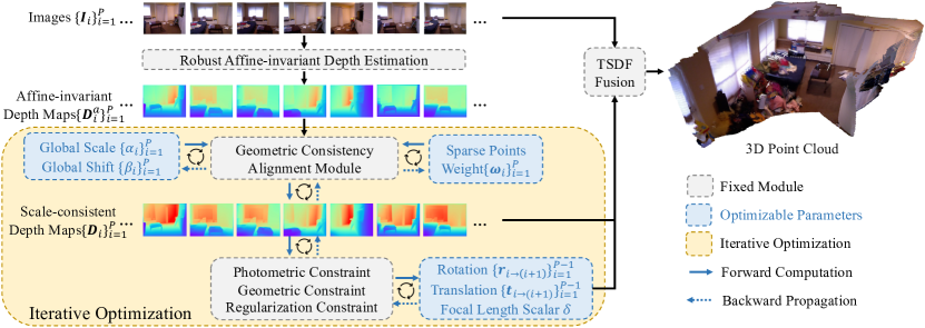
Figure 1: Pipeline. Given a monocular video, we use a frozen, robust monocular depth estimation model to obtain the estimated depths of all frames. Then, we propose a geometric consistency alignment module, which optimizes a sparse set of parameters (i.e., scale, shift, and weight factors) to achieve multi-view geometric consistent depths among all frames. The camera’s intrinsic parameters and poses are also optimized simultaneously. As a result, we achieve high-quality dense 3D reconstruction with optimized depths and camera parameters.

2 Related Work

Learning-based 3D Scene Reconstruction. Learning-based methods [21, 31, 38] rely on a neural network with a large number of learnable parameters to learn the geometry of scenes. Some approaches generate the 3D voxel volume from the 2D image features of the entire sequence [21] or local fragments [31], and estimate an implicit 3D representation from posed images. Besides, some other algorithms [46, 3, 4] attempt to predict poses and depth maps jointly. They employ an ego-motion network and a depth network to predict relative camera poses and depth maps, and supervise the photo-metric consistency [46, 4] and geometric consistency [4].

Multi-view Geometry Based 3D Scene Reconstruction. Multi-view geometry based methods [46, 3, 4, 15, 41, 7, 14] achieve dense 3D reconstruction by finding feature correspondences across views. Traditional methods [26, 27] extract image features, establish correspondences between frames, and optimize the pose and depth iteratively, typically using bundle adjustment [36]. To achieve robust feature representation, some methods leverage plane sweeping to establish correspondences with assumed depth values. They usually construct a cost volume with the CNN-extracted features between images [14, 41, 15] , and employ a ConvNet to predict depth maps after regularization. Compared with those approaches, ours is less likely to suffer from pose catastrophic failures in low-texture regions and can be more robust to diverse scenes.

Besides, visual SLAM systems [19, 20, 6, 10, 11, 12, 25, 35] also estimate the camera motion and construct the map of unknown environments. Methods of [19, 20, 6, 10] rely on the assumption of geometric or photometric consistency to estimate poses and depth through bundle adjustment. Recent works [25, 35] propose to improve the robustness and accuracy by integrating more representative clues and optimization tools from deep learning. These algorithms focus on accurate pose estimation, but may fail to build dense maps with geometry details.

Robust Monocular Depth Estimation. To achieve robust monocular depth estimation, some methods [24, 23, 44, 42] learn the affine-invariant depth with large-scale datasets, which is more likely to be robust to unseen scenarios but up to an unknown scale and shift. Although they achieve promising robustness, the estimated affine-invariant depth needs to recover scale-shift values by globally aligning [24, 23, 44] with ground-truth depth. Some algorithms [18, 16, 17] propose to employ robust depth prediction and achieve visually consistent video depth estimation. In contrast, this work focuses on leveraging robust monocular depth models and aiming at dense 3D scene reconstruction without extra offline-obtained information.

3 Method

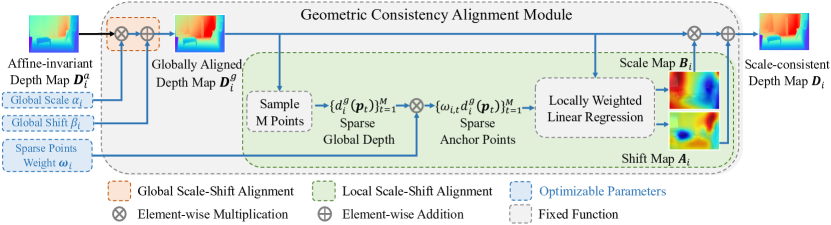
Figure 2: The geometric consistency alignment module. We propose to recover the global scale and shift of depth map first, then apply the locally weighted linear regression method to compute the scale map and shift map, and finally achieve scale-consistent depth.

3.1 Overview

Aiming at 3D reconstruction from a monocular video, we propose a lightweight optimization pipeline to jointly optimize depth maps, camera poses, and intrinsic camera parameters in Figure 1. The core components of our method are the geometric consistency alignment module, optimization objectives, camera parameters initialization, and the keyframe sampling strategy.

With the sampled images $\{\mathbf{I}_{i}\}_{i=1}^{P}$, we first use LeReS [44, 43] to obtain affine-invariant depth maps $\{\mathbf{D}^{a}_{i}\}_{i=1}^{P}$. To avoid disastrous point cloud duplication and distortion, we leverage a geometric consistency alignment module $\mathcal{F}(\cdot,\cdot,\cdot,\cdot)$ to retrieve unknown scale and shift of affine-invariant depth and compute scale-consistent depth $\mathbf{D}_{i}$:

$$\begin{gathered}\mathbf{D}_{i}=\mathcal{F}(\mathbf{D}^{a}_{i};\;\alpha_{i},\beta_{i},\bm{\omega}_{i}),\end{gathered}$$ (1)

where $\alpha_{i}$, $\beta_{i}$, and $\bm{\omega}_{i}$ are the optimization variables.

In order to transfer the robustness of the depth model, three optimization objectives are supervised to ensure multi-frame consistency by warping from source frame $i$ to reference frame $j$. With this warping process, we propose to minimize the color and depth difference between warped points and reference points, i.e., photometric and geometric constraints. An additional regularization constraint is also employed to stabilize the optimization process.

During optimization, the consistency supervision relies on two conditions: 1) the warped reference image and source images must have overlaps; 2) nicely overlapped frames can be automatically selected as our keyframes. Therefore, the appropriate initialization of camera parameters and the keyframes’ sampling strategy are essential.

Finally, with the optimized intrinsic camera parameters, camera poses, and scale-consistent depth maps, we can achieve accurate 3D scene reconstruction with a simple TSDF fusion [45].

3.2 Optimization

We assume a simple pinhole camera model, and use homogeneous representation for all image coordinates. By default, the scale factor in homogeneous coordinate is 1.

Geometric Consistency Alignment Module. The details of geometric consistency alignment module $\mathcal{F}(\cdot)$ are shown in Figure 2. The predicted depths $\{\mathbf{D}^{a}_{i}\}_{i=1}^{P}$ are affine-invariant. The unknown scale and shift will cause duplications and distortions if they are incorrectly estimated. To retrieve them, we perform a two-stage alignment, i.e., a global scale-shift alignment, and a local scale-shift alignment. In the global alignment [44], we optimize for a global scale $\alpha_{i}$ and a global shift $\beta_{i}$ to obtain the globally aligned depth map $\mathbf{D}^{g}_{i}$ as follows:

$$\begin{gathered}\mathbf{D}^{g}_{i}=\alpha_{i}\mathbf{D}^{a}_{i}+\beta_{i}.\\ \end{gathered}$$ (2)

In the local alignment, we compute a scale map $\mathbf{A}_{i}\in\mathbb{R}^{H\times W}$ and shift map $\mathbf{B}_{i}\in\mathbb{R}^{H\times W}$ for each frame $i$ to refine the globally aligned depth. Instead of directly optimizing these two maps, we uniformly sample $M$ sparse global depth $\{d^{g}_{i}({\mathbf{p}_{t}})\}^{M}_{t=1}$ from the globally aligned depth $\mathbf{D}^{g}_{i}$:

$$d^{g}_{i}({\mathbf{p}_{t}})=f_{\rm s}(\mathbf{D}^{g}_{i},\mathbf{p}_{i,t}),\,\,\,\,{\rm for}\,\,t=1...M.$$

where $f_{\text{s}}(\cdot,\cdot)$ retrieves the depth value at a position; e.g., $f_{\rm s}(\mathbf{D}^{g}_{i},\mathbf{p}_{i,t})$ obtains $d^{g}_{i}({\mathbf{p}_{t}})$ from $\mathbf{D}_{i}^{g}$ at the position $\mathbf{p}_{i,t}$. Then, by multiplying sparse global depth $\{d^{g}_{i}({\mathbf{p}_{t}})\}^{M}_{t=1}$ with the weights $\{\omega_{i,t}\}_{t=1}^{M}$, we compute the sparse anchor points $\{\omega_{i,t}\cdot d^{g}_{i}({\mathbf{p}_{t}})\}^{M}_{t=1}$ and use the locally weighted linear regression method[39], i.e., $f_{\text{LWLR}}(\cdot,\cdot)$, to compute the local scale map $\mathbf{A}_{i}\in\mathbb{R}^{H\times W}$ and local shift map $\mathbf{B}_{i}\in\mathbb{R}^{H\times W}$. We also describe the $f_{\text{LWLR}}(\cdot,\cdot)$ module in detail in the supplementary. Such indirect optimization reduces the parameters to ease optimization. The local alignment is as follows.

$$\begin{gathered}\mathbf{A}_{i},\mathbf{B}_{i}=f_{\text{LWLR}}(\mathbf{D}^{g}_{i},\{\omega_{i,t}\cdot d^{g}_{i}({\mathbf{p}_{t}})\}_{t=1}^{M})\\ \mathbf{D}_{i}=\mathbf{A}_{i}\odot\mathbf{D}^{g}_{i}+\mathbf{B}_{i}\end{gathered}$$ (3)

where $\odot$ means element-wise multiplication, and $M$ is set to 25 in our experiments. Therefore, in this module, we only need to optimize for $27$ parameters for each frame, i.e., $\alpha_{i},\beta_{i},\bm{\omega}_{i}$. With our geometric consistency alignment module, we can achieve scale-consistent depth.

Representation of Camera Poses and Intrinsic Camera Parameters. We propose to optimize for the relative rotation vector $\{\mathbf{r}_{i\rightarrow(i+1)}\}_{i=1}^{P-1}$ (i.e., Euler angles) and relative translation vector $\{\mathbf{t}_{i\rightarrow(i+1)}\}_{i=1}^{P-1}$ between two adjacent frames. They are initialized to 0 and are transformed to $4\times 4$ relative pose matrices $\{\mathbf{P}_{i\rightarrow(i+1)}\}_{i=1}^{P-1}$ with $\mathcal{H}(\cdot,\cdot)$. The relative pose matrices $\{\mathbf{P}_{i\rightarrow(i+1)}\}_{i=1}^{P-1}$ are transformed into camera-to-world poses matrices $\{\mathbf{P}_{i}\}_{i=1}^{P}$ with the product operation. Such initialization ensures the initial overlap of keyframes. For intrinsic camera parameters, we assume a simple pinhole camera model, initialize the focal length to be $f_{0}=1.2\cdot\max(H,W)$, and learn the focal length with a learnable scalar $\delta$. We assume that the optical center is at the image center. Thus for camera parameters, we need to optimize for $6(P-1)+1$ variables:

$$\begin{gathered}\mathbf{P}_{i\rightarrow(i+1)}=\mathcal{H}(\mathbf{r}_{i\rightarrow(i+1)},\mathbf{t}_{i\rightarrow(i+1)}),\;\;\;\mathbf{P}_{1}=\mathbf{E}_{4,4},\\ \mathbf{P}_{i}=\mathbf{P}_{1}\prod_{k=1}^{i-1}\mathbf{P}_{k\rightarrow(k+1)},\;\;\;\mathbf{K}=\begin{bmatrix}\delta f_{0}&0&\nicefrac{{W}}{{2}}\\ 0&\delta f_{0}&\nicefrac{{H}}{{2}}\\ 0&0&1\end{bmatrix}\end{gathered}$$ (4)

where $\mathbf{E}_{4,4}$ is the $4\times 4$ elementary matrix.

Optimization Objectives. The image coordinate $\mathbf{p}_{i}$ in frame $i$ can be wrapped to frame $j$ as follows.

$$\begin{gathered}f_{\text{s}}(\mathbf{D}_{i\rightarrow j},\mathbf{p}_{i})\mathbf{p}_{i\rightarrow j}=\mathbf{K}\mathbf{R}_{j}^{\mathsf{T}}\bigl{[}\mathbf{R}_{i}\mathbf{K}^{-1}f_{\text{s}}(\mathbf{D}_{i},\mathbf{p}_{i})\mathbf{p}_{i}+\mathbf{t}_{i}-\mathbf{t}_{j}\bigr{]},\\ \mathbf{p}_{i},\mathbf{p}_{i\rightarrow j},\mathbf{t}_{i},\mathbf{t}_{j}\in\mathbb{R}^{3\times 1},\;\;\;\mathbf{R}_{i},\mathbf{R}_{j},\mathbf{K}\in\mathbb{R}^{3\times 3}\end{gathered}$$ (5)

where $\mathbf{K}$ is the intrinsic camera parameter. $\mathbf{R}_{i}$ and $\mathbf{t}_{i}$ are the camera-to-world rotation and translation matrices, and $\mathbf{P}_{i}=\begin{bmatrix}\mathbf{R}_{i}&\mathbf{t}_{i}\\ \mathbf{0}&1\end{bmatrix}$. $\mathbf{p}_{i\rightarrow j}$ is the point warped from $\mathbf{p}_{i}$ of frame $i$ to frame $j$, and $\mathbf{D}_{i\rightarrow j}$ is the warped depth map.

To optimize the proposed variables including $\{\alpha_{i}\}_{i=1}^{P}$, $\{\beta_{i}\}_{i=1}^{P}$, $\delta$, $\{\mathbf{r}_{i\rightarrow(i+1)}\}_{i=1}^{P-1}$, $\{\mathbf{t}_{i\rightarrow(i+1)}\}_{i=1}^{P-1}$, and $\{\bm{\omega}_{i}\}_{i=1}^{P}$, we propose to use the pixel-wise photometric and geometric constraint [3] together to ensure the consistency of color and depth along the video as follows.

$$L_{pc}=\frac{1}{\left|V\right|}\sum_{\mathbf{p}\in V\atop(i,j)\in K}\lvert f_{\text{s}}(\mathbf{I}_{i},\mathbf{p}_{i})-f_{\text{s}}(\mathbf{I}_{j},\mathbf{p}_{i\rightarrow j})\rvert$$ (6)

$$L_{gc}=\frac{1}{\left|V\right|}\sum_{\mathbf{p}\in V\atop(i,j)\in K}\frac{\left|f_{\text{s}}(\mathbf{D}_{j},\mathbf{p}_{i\rightarrow j})-f_{\text{s}}(\mathbf{D}_{i\rightarrow j},\mathbf{p}_{i})\right|}{f_{\text{s}}(\mathbf{D}_{j},\mathbf{p}_{i\rightarrow j})+f_{\text{s}}(\mathbf{D}_{i\rightarrow j},\mathbf{p}_{i})}$$ (7)

where $V$ represents all valid points successfully projected from frame $i$ to frame $j$, $K$ is the selected keyframe pairs.

Furthermore, we enforce a regularization term on the sampled sparse anchor points:

$$\begin{gathered}L_{regu}=\sum_{i=1}^{N}\sum_{t=1}^{M}\left|1-\omega_{i,t}\right|\end{gathered}$$ (8)

The overall constraints are as follows.

$$\begin{gathered}L=\lambda_{pc}L_{pc}+\lambda_{gc}L_{gc}+\lambda_{regu}L_{regu}\end{gathered}$$ (9)

where $\lambda_{pc}$, $\lambda_{gc}$, and $\lambda_{regu}$ are weights to balance them.

Optimization Details. Before we perform optimization, we first sample $P$ frames from the video to reduce the time complexity. With these sampled frames, we perform the keyframes sampling and optimization, which consists of two stages, i.e., local keyframes sampling for optimization, and global keyframes sampling for optimization.

Local keyframes sampling and optimization. In optimization, we first sample local keyframes from the $k$ nearest frames of each reference frame. $k$ is set to $6$ in our experiments. To reduce computation time complexity, we do not use all these local keyframes with the current frame but select them based on probability. The probability for each keyframe is set as follows.

$$\begin{gathered}p_{l}=\left\{\begin{aligned} \frac{1}{k},&\,\,{\rm if}\,k\text{-}{\rm nearest~{}neighbors},\\ 0,&~{}~{}{\rm otherwise},\end{aligned}\right.\end{gathered}$$ (10)

where $p_{l}$ is the keyframe sample probability.

Algorithm 1 Optimization Algorithm

0:  $N$ images $\{\mathbf{I}_{i}\}_{i=1}^{N}$

0:  scale-consistent depth maps $\{\mathbf{D}_{i}\}_{i=1}^{P}$, intrinsic camera parameter $\mathbf{K}$, camera-to-world camera poses $\{\mathbf{P}_{i}\}_{i=1}^{P-1}$

1:  Sample $P$ images $\{\mathbf{I}_{i}\}_{i=1}^{P}$ from $\{\mathbf{I}_{i}\}_{i=1}^{N}$

2:  Obtain affine-invariant depth $\{\mathbf{D}^{a}_{i}\}_{i=1}^{P}$ from $\{\mathbf{I}_{i}\}_{i=1}^{P}$

3:  Initialize the global scale $\{\alpha_{i}\}_{i=1}^{P}$, global shift $\{\beta_{i}\}_{i=1}^{P}$, focal length scalar $\delta$, relative rotation $\{\mathbf{r}_{i\rightarrow(i+1)}\}_{i=1}^{P-1}$, relative translation $\{\mathbf{t}_{i\rightarrow(i+1)}\}_{i=1}^{P-1}$, sparse points weight $\{\bm{\omega}_{i}\}_{i=1}^{P}$

4:  for $stage$ in [$Local$, $Global$] do

5:     for $iter$ = 1 to $iterations$ do

6:        Compute $\{\mathbf{P}_{i}\}_{i=1}^{P-1}$ and $\mathbf{K}$ with Eq. (4)

7:        if $stage$ = $Local$ then

8:           Sample keyframe pairs $\{(i_{k},j_{k})\}_{k=1}^{K}$ with Eq. (10)

9:        else

10:           Sample keyframe pairs $\{(i_{k},j_{k})\}_{k=1}^{K}$ with Eq. (11)

11:        end if

12:        for keyframe pair $(i,j)$ in $\{(i_{k},j_{k})\}_{k=1}^{K}$ do

13:           Compute scale-consistent depth $\mathbf{D}_{i}$, $\mathbf{D}_{j}$ with Eq. (3);

14:           Warp $\mathbf{p}_{i}$ from frame $i$ to frame $j$, get warped depth $\mathbf{D}_{i\rightarrow j}$ and warped locations $\mathbf{p}_{i\rightarrow j}$ with Eq. (5)

15:           Compute optimization objectives with Eq. (9)

16:        end for

17:        Back-propagate and update $\{\alpha_{i}\}_{i=1}^{P}$, $\{\beta_{i}\}_{i=1}^{P}$, $\delta$, $\{\mathbf{r}_{i\rightarrow(i+1)}\}_{i=1}^{P-1}$, $\{\mathbf{t}_{i\rightarrow(i+1)}\}_{i=1}^{P-1}$, $\{\bm{\omega}_{i}\}_{i=1}^{P}$

18:     end for

19:  end for

20:  Compute scale-consistent depth maps $\{\mathbf{D}_{i}\}_{i=1}^{P}$ with Eq. (3), compute camera parameters $\mathbf{K}$ and $\{\mathbf{P}_{i}\}_{i=1}^{P-1}$ with Eq. (4)

Table 1: Quantitative comparison of zero-shot 3D scene reconstruction with state-of-the-art methods. We compare with seven categories of reconstruction algorithms on several video sequences of five unseen datasets: NYU [29], ScanNet [9], 7-Scenes [28], TUM [30], and KITTI [13]. Note that NeuralRecon is trained on ScanNet [9], ^∗ denotes ground-truth camera poses are given, and “Rank” means the average ranking performance of each column. We evaluate the Chamfer distance C-$l_{1}$ and the F-score with a threshold of 5cm. As a result, our method achieves state-of-the-art rank on the five zero-shot datasets.

Method	NYU [29]		ScanNet [9]		7-Scenes [28]		TUM [30]		KITTI [13]		Rank
	C-$l_{1}$ $\downarrow$	F-score$\uparrow$	C-$l_{1}$ $\downarrow$	F-score$\uparrow$	C-$l_{1}$ $\downarrow$	F-score$\uparrow$	C-$l_{1}$ $\downarrow$	F-score$\uparrow$	C-$l_{1}$ $\downarrow$	F-score$\uparrow$
NeuralRecon∗ [31]	0.487	0.185	trained on ScanNet		0.235	0.219	0.435	0.241	failed on KITTI		8.125
DPSNet∗ [15]	0.198	0.391	0.299	0.266	0.574	0.142	0.336	0.263	0.290	0.232	4.800
BoostingDepth-DROID [39]	0.139	0.481	0.379	0.292	0.235	0.460	0.322	0.439	2.431	0.010	3.600
SC-DepthV3 [32]	0.196	0.458	0.402	0.214	0.252	0.240	0.525	0.244	4.133	0.036	5.500
CVD [18]	0.471	0.302	failed on ScanNet		0.416	0.215	0.378	0.239	5.479	0.029	7.900
RCVD [16]	0.303	0.346	0.641	0.125	0.497	0.182	0.679	0.218	58.372	0.020	8.300
GCVD [17]	0.148	0.453	0.631	0.147	0.196	0.326	0.350	0.339	2.127	0.114	4.400
COLMAP [26, 27]	0.251	0.343	0.796	0.127	0.513	0.178	0.385	0.249	107.451	0.152	7.300
DROID-SLAM [35]	0.224	0.516	0.416	0.384	0.304	0.469	0.285	0.433	0.686	0.155	3.200
Ours	0.099	0.622	0.170	0.410	0.170	0.464	0.211	0.453	0.670	0.151	1.500

Table 2: Quantitative comparison of zero-shot depth estimation with state-of-the-art methods. We evaluate the absolute relative error (AbsRel) and percentage of accurate depth pixels ($\delta_{1}$) on several videos of five unseen datasets. “Rank” means the average ranking performance of each column. The gray “LeReS” represents the performance of affine-invariant depth without any alignment with ground-truth depth. As a result, our algorithm achieves state-of-the-art rank performance.

Method	NYU [29]		ScanNet [9]		7-Scenes [28]		TUM [30]		KITTI [13]		Rank
	AbsRel$\downarrow$	$\delta_{1}$$\uparrow$	AbsRel$\downarrow$	$\delta_{1}$$\uparrow$	AbsRel$\downarrow$	$\delta_{1}$$\uparrow$	AbsRel$\downarrow$	$\delta_{1}$$\uparrow$	AbsRel$\downarrow$	$\delta_{1}$$\uparrow$
DPSNet∗ [15]	0.200	0.662	0.216	0.630	0.201	0.657	0.331	0.457	0.188	0.729	6.4
BoostingDepth-DROID [39]	0.096	0.921	0.236	0.685	0.145	0.828	0.180	0.742	0.112	0.860	2.7
SC-DepthV3 [32]	0.120	0.858	0.197	0.672	0.188	0.688	0.254	0.569	0.287	0.463	5.2
CVD [18]	0.167	0.837	failed on ScanNet		0.180	0.847	0.148	0.797	0.717	0.215	5.6
RCVD [16]	0.192	0.700	0.235	0.620	0.241	0.635	0.246	0.612	0.220	0.606	6.6
GCVD [17]	0.163	0.768	0.316	0.527	0.203	0.650	0.248	0.697	0.240	0.543	6.4
COLMAP [27, 26]	0.233	0.722	0.562	0.409	0.268	0.666	0.269	0.665	0.302	0.773	7.2
DROID-SLAM [35]	0.143	0.847	0.210	0.773	0.154	0.827	0.210	0.720	0.115	0.914	3.1
LeReS [44]	0.277	0.508	0.409	0.339	0.414	0.345	0.445	0.320	0.298	0.439	-
Ours	0.092	0.923	0.127	0.858	0.135	0.844	0.145	0.799	0.203	0.632	1.8

Table 3: Quantitative comparison of zero-shot pose estimation. “ATE”, “RPE-T”, and “RPE-R” stand for the absolute trajectory error and the relative pose error of translation and rotation consecutively. “%” represents the percentage of successfully tracked frames. Note that ORB-SLAM3 fails to track the trajectory on some low-texture regions, and can only estimate partial camera poses. Our algorithm achieves comparable performance to ORB-SLAM3 on three unseen datasets and better performance than the video depth estimation algorithms.

Method	GT	NYU [29]				ScanNet [9]				7-Scenes [28]				TUM [30]				KITTI [13]
	Intrinsic	ATE$\downarrow$	RPE-T$\downarrow$	RPE-R$\downarrow$	%$\uparrow$	ATE$\downarrow$	RPE-T$\downarrow$	RPE-R$\downarrow$	%$\uparrow$	ATE$\downarrow$	RPE-T$\downarrow$	RPE-R$\downarrow$	%$\uparrow$	ATE$\downarrow$	RPE-T$\downarrow$	RPE-R$\downarrow$	%$\uparrow$	ATE$\downarrow$	RPE-T$\downarrow$	RPE-R$\downarrow$	%$\uparrow$
SC-DepthV3 [32]	✓	0.241	0.444	0.115	1.000	0.492	0.702	0.327	1.000	1.011	1.644	0.389	1.000	0.528	0.787	0.399	1.000	1.796	4.186	0.077	1.000
CVD [18]	✓	1.192	2.049	0.107	1.000	0.734	1.197	0.257	1.000	0.532	1.644	0.378	1.000	0.268	0.844	0.447	1.000	19.32	24.50	0.027	1.000
RCVD [16]		0.460	1.263	0.114	1.000	1.025	1.708	0.615	1.000	0.559	1.545	0.394	1.000	0.626	1.083	0.421	1.000	134.3	160.7	0.463	1.000
GCVD [17]		0.160	0.237	0.083	1.000	0.573	0.979	0.620	1.000	0.259	0.368	0.162	1.000	0.162	0.204	0.113	1.000	5.678	8.733	0.089	1.000
COLMAP [27, 26]		0.091	0.137	0.055	1.000	0.352	0.426	0.096	1.000	0.062	0.090	0.051	1.000	0.075	0.102	0.064	1.000	3.707	3.454	0.016	1.000
DROID-SLAM [35]	✓	0.050	0.079	0.032	1.000	0.230	0.230	0.052	1.000	0.050	0.072	0.072	1.000	0.044	0.077	0.079	1.000	1.491	2.302	0.005	1.000
ORB-SLAM3 [6]	✓	0.065	0.097	0.039	0.791	0.208	0.300	0.098	0.426	0.118	0.211	0.121	0.956	0.104	0.144	0.082	0.504	3.124	3.926	0.009	0.971
Ours		0.079	0.121	0.046	1.000	0.130	0.184	0.085	1.000	0.141	0.229	0.075	1.000	0.176	0.228	0.151	1.000	3.541	5.663	0.053	1.000

Table 4: Quantitative comparison of zero-shot intrinsic camera parameter estimation. “FOV AbsRel” represents the absolute relative error of the field of view. Note that only three algorithms can estimate the intrinsic camera parameter from the input video, and our algorithm can achieve accurate and robust performance on four unseen datasets.

Method	NYU [29]	ScanNet [9]	7-Scenes [28]	TUM [30]	Rank
	FOV AbsRel$\downarrow$	FOV AbsRel$\downarrow$	FOV AbsRel$\downarrow$	FOV AbsRel$\downarrow$
RCVD [16]	0.144	0.148	0.110	0.174	2.75
GCVD [17]	0.015	0.126	0.143	0.043	1.75
Ours	0.032	0.032	0.085	0.056	1.50

Global keyframes sampling and optimization. We further perform global keyframes sampling and optimization to improve long-range consistency. For each reference frame, all other frames are regarded as paired keyframes, but they are labeled with different sampling probabilities. We compute the relative pose between each reference frame $\mathbf{I}_{i}$ and any other frame $\mathbf{I}_{j}$. Based on the relative pose angle $\theta_{ij}$, we set the global sampling probability $p_{g}$ as follows.

$$\begin{gathered}p_{g}=\frac{p_{l}+p}{2},p=\left\{\begin{aligned} \frac{\theta_{ij}}{\phi^{2}},&\;\;{\rm if}\;0<\theta_{ij}\leq\phi\\ \frac{2}{\phi}-\frac{\theta_{ij}}{\phi^{2}},&\;\;{\rm if}\;\phi<\theta_{ij}<2\phi\\ 0,&\;\;{\rm otherwise}\\ \end{aligned}\right.\end{gathered}$$ (11)

where $\phi$ is an angle threshold, and $\theta_{ij}$ is the relative rotation angle between the source frame $\mathbf{I}_{i}$ and the reference frame $\mathbf{I}_{j}$. $p_{l}$ is the local probability with Eq. (10). The optimization is summarized in Algorithm 1.

4 Experiments

We evaluate the 3D reconstruction, scale-consistent depths, optimized camera poses, and optimized intrinsic camera parameters in experiments. More details and analyses including runtime can be found in the supplementary.

4.1 Dense 3D Scene Reconstruction

To show the robustness and accuracy of our reconstruction method, we compare it with a learning-based volumetric 3D reconstruction method (NeuralRecon [31]), a multi-view depth estimation method (DPSNet [15]), a per-frame scale-shift alignment method (BoostingDepth [39]), an unsupervised video depth estimation method (SC-DepthV3 [32]), some consistent video depth estimation methods (CVD [18], RCVD [16], GCVD [17]), a Structure-from-Motion method COLMAP [27, 26], and a robust deep visual SLAM method (DROID-SLAM [35]) on several video sequences of $5$ zero-shot datasets, i.e., NYU [29], ScanNet [9], 7-Scenes [28], TUM [30], KITTI [13]. Note that NeuralRecon is trained on ScanNet, while others are evaluated on unseen scenarios. NeuralRecon and DPSNet require GT poses and camera intrinsic as input, and SC-DepthV3, CVD, and DROID-SLAM require camera intrinsic. For fair comparison, we employ the estimated poses and depths of DROID-SLAM for BoostingDepth (BoostingDepth-DROID) to iteratively align the scale-shift values and filter outliers, as their paper does. Other methods optimize camera parameters on their own.

Quantitative comparisons of zero-shot 3D reconstruction and depth are shown in Table 1 and Table 2 respectively. NeuralRecon [31], DPSNet [15], SC-DepthV3 [32] need to optimize millions of parameters, thus showing less robustness to unseen datasets. Rather than purely per-frame aligning with offline-obtained depth after filtering as BoostingDepth  [39] does, we jointly optimize the camera parameters and depth parameters, which ensures consistency between frames and less suffers from outliers of sparse points. CVD [18] fails to reconstruct half of the ScanNet scenarios. Compared with RCVD [16], and GCVD [17], our method employs a global and a local scale-shift recovery strategy, which can rectify the affine-invariant depth to a much more accurate scale-consistent depth. Thus, we can achieve much more accurate reconstructions. The COLMAP [27, 26] struggles to estimate dense depth maps, and thus results in sparse 3D reconstruction. The robust DROID-SLAM [35] focuses on optimizing more robust poses and trajectories with the recurrent module, and spends less effort on dense reconstruction. Thus, their dense reconstruction is more likely to suffer from outliers. In contrast, our optimization is based on dense depth priors and employs a global and local optimization strategy to reduce noise, thus we in general achieve better reconstruction performance.

Table 5: Runtime analysis on three representative scenes. Our pipeline achieves state-of-the-art reconstruction but only takes around a quarter of an hour to optimize.

Method	basement_0001a	bedroom_0015	chess
NeuralRecon[31]	-	-	-
DPSNet[15]	5m 53s	45s	12m 20s
BoostingDepth-DROID[39]	35s	10s	47s
SC-DepthV3[32]	1m 47s	17s	1m 54s
CVD[18]	1h 7m 6s	12m 30s	8h 1m 34s
RCVD[16]	1h 15m 45s	10m 6s	6h 14m 54s
GCVD[17]	10m 26s	2m 37s	52m 15s
DROID-SLAM[35]	35s	16s	1m 18s
COLMAP[26, 27]	50m 44s	8m 34s	9h 40m 49s
Ours	14m 55s	6m 55s	21m 8s

Quantitative comparisons of zero-shot pose estimation and intrinsic camera parameter estimation are shown in Table 3 and Table 4. Our algorithm achieves comparable performance with the traditional SLAM methods ORB-SLAM3 [6] on three datasets. However, the ORB-SLAM3 can only estimate the camera poses of partial frames due to the failure of tracking features. In contrast, our algorithm can optimize and interpolate to obtain dense trajectories. Compared to four video depth estimation methods, we can outperform them by a large margin. Note that only ours, RCVD, and GCVD can optimize the intrinsic camera parameters, while others can only employ GT camera intrinsic as input. For intrinsic camera parameter estimation, our algorithm can achieve robust and accurate performance on four unseen datasets.

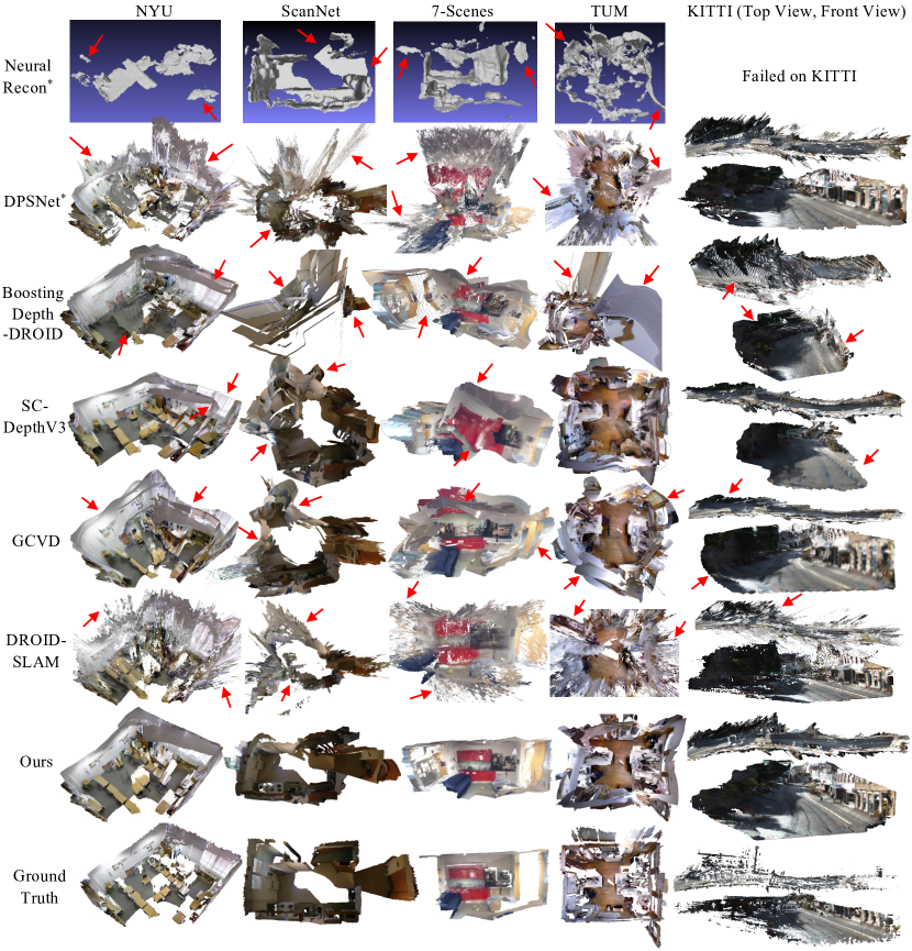
Figure 3: Qualitative comparison of zero-shot 3D scene reconstruction from a monocular video. We compare with five representative algorithms on five unseen datasets. Note that NeuralRecon is trained on ScanNet [9] and can only output uncolored mesh, and ^∗ represents the employment of ground-truth camera poses during reconstruction. These methods either suffer from inaccurate pose estimation, or predict noise depth maps (please see the red arrows). As can be seen, our algorithm can reconstruct better 3D scene shape without any offline-computed camera parameters.

Qualitative comparisons are reported in Figure. 3. NeuralRecon can only reconstruct partial meshes of unseen scenarios. The DPSNet [15] suffers from inaccurate feature correspondences, which cause noisy point clouds. BoostingDepth [39] can only filter out inaccurate points of DROID-SLAM but cannot ensure the temporal consistency, and thus fails to reconstruct consistent mesh. The SC-DepthV3 [32] suffers from the weak supervision of photometric loss and work worse on some low-texture regions. Consistent video depth estimation methods such as GCVD [17] can not recover the shift of depth maps, which will cause distortions in 3D point clouds. DROID-SLAM [35] concentrates on accurate pose estimation but does not work well for dense reconstruction, and thus suffering from outliers. In contrast, our method can achieve more robust and accurate 3D scene reconstruction, without requiring offline-acquired camera poses and camera intrinsic parameters.

For quantitative efficiency analysis, the runtime comparisons on 40 Intel Xeon Silver 4210 CPUs and an RTX 3090 Ti GPU are presented in Table 5, which includes three representative scenes with 225, 48, and 1000 images, respectively. Our pipeline achieves state-of-the-art reconstruction while only taking about a quarter of an hour to optimize, even for 1000 images. Note that only the time of predicting depth and poses without RGB-D fusion are recorded.

4.2 Ablation Study

We carry out ablation experiments in terms of essential components of our algorithm to evaluate their effectiveness.

Table 6: Comparison of geometric consistency alignment mechanisms on the NYU [29] dataset. “w/ deform.” means optimizing the flexible deformation map of RCVD [16] as a replacement for our alignment module. “baseline” means directly optimizing the per-frame pixel-wise depth map without the affine-invariant depth priors. As a result, the employment of our geometric consistency alignment module contributes significantly to the optimization.

Method	Depth		Pose			Reconstruction
	AbsRel$\downarrow$	$\delta_{1}$$\uparrow$	ATE$\downarrow$	RPE-T$\downarrow$	RPE-R$\downarrow$	C-$l_{1}$$\downarrow$	F-score$\uparrow$
Ours	0.092	0.923	0.096	0.144	0.053	0.099	0.622
w/ deform. [16]	0.153	0.771	0.145	0.290	0.082	0.160	0.470
baseline	0.350	0.466	0.710	1.097	0.215	0.285	0.303

Table 7: Comparison of optimization objectives on the ScanNet [9] dataset. The photometric constraint supervises the color consistency, the geometric constraint ensures the multi-view geometry consistency, and the regularization constraint stabilizes the convergence of optimization. As a result, the three components of our optimization objectives are all important.

Method	Depth		Pose			Reconstruction
	AbsRel$\downarrow$	$\delta_{1}$$\uparrow$	ATE$\downarrow$	RPE-T$\downarrow$	RPE-R$\downarrow$	C-$l_{1}$$\downarrow$	F-score$\uparrow$
Ours	0.127	0.858	0.271	0.348	0.147	0.170	0.410
w/o photo.	0.219	0.636	1.722	2.331	1.039	0.775	0.169
w/o geo.	0.168	0.750	0.316	0.404	0.179	0.211	0.323
w/o regu.	0.226	0.603	0.245	0.338	0.189	0.220	0.254

Geometric Consistency Alignment Module. Table 6 shows the performance of different geometric consistency alignment modules. Previous consistent video depth methods RCVD and GCVD employ flexible deformation maps (“w/ deform.”) and aim for more accurate scale-consistent depth. However, they both ignore the shift issues in affine-invariant depth, which is pretty significant in the 3D reconstruction task. By contrast, our method (“Ours”) proposes a global and local scale shift alignment module for depth rectification. We also compare with a baseline method (“baseline”), which directly optimizes all frames’ pixel-wise depths without the affine-invariant depth priors. All depths are initialized to 1. Our alignment module works much better than previous methods.

Optimization Objectives. To evaluate the effectiveness of each constraint employed in our method, we propose to remove them one by one, and the results are shown in Table 7. We can see that without the photometric constraint or geometric constraint, the performance will degrade a lot. When removing the regularization term, the accuracy of the pose, depth, and reconstruction will also decrease.

Effectiveness of Optimization Stages. Our optimization algorithm is composed of local keyframes optimization (“Local”) and global keyframes optimization (“Global”). The local stage endures the local consistency between the nearest $k$ keyframes, and can reconstruct roughly accurate 3D scene shapes. The global stage selects long-range keyframes to supervise global consistency. As shown in Table 8, the reconstruction performance improves gradually.

5 Conclusion

In this paper, we have presented an effective pipeline to realize 3D scene reconstruction by leveraging the robustness of affine-invariant depth estimation, freezing the depth model, and jointly optimizing dozens of depth and camera parameters for each frame. Due to the sparsity of parameters, our pipeline can transfer the robustness of seemingly weak depth geometry prior to diverse scenes. Extensive experiments show that our pipeline can achieve robust dense 3D reconstruction on challenging unseen scenes.

Table 8: Effectiveness of our two-stage keyframe sampling and optimization strategy. The “Local” stage ensures consistency between the nearest $k$ keyframes. The “Global” stage samples keyframes globally with different sampling probabilities according to the optimized relative poses. As a result, with the coarse-to-fine optimization strategy, our algorithm achieves better performance. The experiment is performed on NYU [29] dataset.

Stage	Depth		Pose			Reconstruction
	AbsRel$\downarrow$	$\delta_{1}\uparrow$	ATE$\downarrow$	RPE-T$\downarrow$	RPE-R$\downarrow$	C-$l_{1}$ $\downarrow$	F-score$\uparrow$
Local	0.111	0.884	0.111	0.179	0.068	0.091	0.593
Global	0.092	0.923	0.096	0.144	0.053	0.099	0.622

Supplementary Material

Appendix A Details About the LWLR Module

Given a globally aligned depth map $\bm{D}^{g}$ and sparse guided points $\bm{y}$, the LWLR module[39] recovers a location-aware scale-shift map. Concretely, for each 2D coordinate $(u,v)$, the sampled globally aligned depth $\bm{d}$ can be fitted to the ground-truth depth $\bm{y}$ by minimizing the squared locally weighted $\ell_{2}$ distance, which is re-weighted by a diagonal weight matrix $\bm{W}_{u,v}$.

$$\begin{gathered}\mathop{\min}\limits_{\bm{\beta}_{u,v}}~{}~{}(\bm{y}-\bm{X}\bm{\beta}_{u,v})^{\mathsf{T}}\bm{W}_{u,v}(\bm{y}-\bm{X}\bm{\beta}_{u,v})+\lambda\theta_{u,v}^{2}\\ \bm{W}_{u,v}=diag(w_{1},w_{2},...,w_{m}),~{}w_{i}=\frac{1}{\sqrt{2\pi}}\exp(-\frac{{\rm dist}_{i}^{2}}{2b^{2}})\\ \bm{\hat{\beta}}_{u,v}=(\bm{X}^{\mathsf{T}}\bm{W}_{u,v}\bm{X}+\bm{A})^{-1}\bm{X}^{\mathsf{T}}\bm{W}_{u,v}\bm{y}\\ \bm{A}=\begin{bmatrix}\lambda&0\\ 0&0\end{bmatrix},~{}\bm{D}=\bm{S}\odot\bm{D}^{g}+\bm{\Theta}\\ \bm{X}=[\bm{d}^{\mathsf{T}},\bm{1}]\ \in{\cal R}^{m\times 2},~{}~{}\bm{\beta}_{u,v}=[s_{u,v},\theta_{u,v}]^{\mathsf{T}}\in{\cal R}^{2\times 1}\\ \bm{D},\bm{S},\bm{D}^{g},\bm{\Theta}\in{\cal R}^{H\times W},~{}~{}\bm{d},\bm{y}\in{\cal R}^{m\times 1}\\ \end{gathered}$$ (12)

where $\bm{y}$ is the sampled sparse ground-truth metric depth, $\bm{d}$ is the sampled globally aligned depth, whose 2D coordinates are the same with those of sparse guided points $\bm{y}$. $\bm{X}$ is the homogeneous representation of $\bm{d}$, $m$ stands for the number of sampled points. $b$ is the bandwidth of Gaussian kernel, and ${\rm dist}_{i}$ is the Euclidean distance between the the coordinate $(u_{i},v_{i})$ of $i$-th guided point and target point $(u,v)$. $\lambda$ is a $l_{2}$ regularization hyperparameter used for restricting the solution to be simple. By iterating the target point $(u,v)$ over the whole image, the scale map $\bm{S}$ and shift map $\bm{\Theta}$ can be generated composed of the scale values $s_{u,v}$ and shift values $\theta_{u,v}$ of each location $(u,v)$. Finally, the locally recovered metric depth $\bm{\hat{D}}$ equals to the shift map $\bm{\Theta}$ plus the Hadamard product ($\odot$, known as element-wise product) of the affine-invariant depth $\bm{D}$ and the scale map $\bm{S}$. The operation above can be summarized as below.

$$\begin{gathered}\bm{S},\bm{\Theta}=f_{\text{LWLR}}(\bm{D}^{g},\bm{y})\\ \bm{D}=\bm{S}\odot\bm{D}^{g}+\bm{\Theta}\end{gathered}$$ (13)

Rather than relying on sparse ground-truth metric depth $\bm{y}$, we replace it with $\{\omega_{i,t}\cdot d^{g}_{i}({\mathbf{p}_{t}})\}^{M}_{t=1}$, which is related to parameters $\{\omega_{i,t}\}_{t=1}^{M}$ and sampled sparse global depth $\{d^{g}_{i}({\mathbf{p}_{t}})\}^{M}_{t=1}$. By ensuring multi-frame consistency, we can retrieve scale-consistent depth maps.

$$\begin{gathered}\mathbf{A}_{i},\mathbf{B}_{i}=f_{\text{LWLR}}(\mathbf{D}^{g}_{i},\{\omega_{i,t}\cdot d^{g}_{i}({\mathbf{p}_{t}})\}_{t=1}^{M})\\ \mathbf{D}_{i}=\mathbf{A}_{i}\odot\mathbf{D}^{g}_{i}+\mathbf{B}_{i}\end{gathered}$$ (14)

Appendix B Efficiency of Photometric Constraint

Furthermore, we also explore the efficiency of the photometric constraint on the NYU[29] dataset. We supervise the consistency of coordinates warped by the optical flow and the optimized parameters, as a replacement for photometric constraint. As shown in Table S1, although comparable performance can the flow-guided constraint achieve, it relies on predicting dense optical flow between every two frames with a robust model RAFT[34], which can be time-consuming due to the recurrent refinement model and the $O(N^{2})$ time complexity. In contrast, the photometric constraint does not require offline-computed optical flow and can be more efficient, especially on long-form videos.

Appendix C Keyframe Sampling Strategy

We sample the keyframes with the optical flow computed with RAFT, and compare it with ours on the NYU dataset. The flow-guided keyframes will be selected if the valid regions are larger than 30 percent after checking the forward-backward consistency. As shown in Table S2, our algorithm is more efficient and even outperforms the flow-guided keyframe sampling strategy due to the pose-based long-range keyframe sampling.

Table S1: Efficiency of the photometric constraint. We simply replace the photometric constraint with spatial constraint (“w/ flow”), and supervises the coordinates consistency warped by optical flow[34] and optimized parameters. Although comparable performance can it achieve, predicting dense optical flows with a deep network between every two frames is computationally expensive and time-consuming. Our algorithm can be more efficient while remains comparable performance.

Method	Time	Depth		Pose			Reconstruction
	Complexity	AbsRel$\downarrow$	$\delta_{1}\uparrow$	ATE$\downarrow$	RPE-T$\downarrow$	RPE-R$\downarrow$	C-$l_{1}$ $\downarrow$	F-score$\uparrow$
Ours	$O(1)$	0.092	0.923	0.096	0.144	0.053	0.099	0.622
w/ flow	$O(N^{2})$	0.102	0.907	0.095	0.155	0.052	0.085	0.627

Table S2: Keyframe sampling strategy. We sample keyframes according to the valid regions of the estimated optical flow. As a result, our algorithm not only spends less time but also achieves better performance.

Method	Time	Depth		Pose			Reconstruction
	Complexity	AbsRel$\downarrow$	$\delta_{1}\uparrow$	ATE$\downarrow$	RPE-T$\downarrow$	RPE-R$\downarrow$	C-$l_{1}$ $\downarrow$	F-score$\uparrow$
Ours	$O(1)$	0.092	0.923	0.096	0.144	0.053	0.099	0.622
w/ flow keyframe	$O(N^{2})$	0.103	0.897	0.174	0.262	0.113	0.155	0.565

Appendix D Upper Bound Analysis

Our optimization can work better if accurate GT poses and intrinsics are given. As shown in Table S3, the performance on the NYU dataset remains nearly the same with known GT intrinsic. With known GT poses, the quality of depth, pose, and reconstruction can be improved compared to video-only optimization. With both GT poses and intrinsic, the performance can achieve slightly better results.

Table S3: Upper bound analysis. With known GT poses, our algorithm can achieve better performance. The GT intrinsic alone does not improve the reconstruction performance , but can achieve slight performance improvement together with GT poses.

GT intrinsic	GT poses	Depth		Pose			Reconstruction
		AbsRel$\downarrow$	$\delta_{1}\uparrow$	ATE$\downarrow$	RPE-T$\downarrow$	RPE-R$\downarrow$	C-$l_{1}$ $\downarrow$	F-score$\uparrow$
		0.092	0.923	0.096	0.144	0.053	0.099	0.622
✓		0.092	0.920	0.095	0.147	0.050	0.103	0.622
	✓	0.085	0.933	-	-	-	0.070	0.662
✓	✓	0.081	0.938	-	-	-	0.064	0.674

Appendix E Analysis of Optimization Objectives

Our optimization objectives are composed of photometric constraint, geometric constraint, and regularization constraint. The photometric constraint $L_{pc}$ ensures the color consistency between the reference frame and the warped source frame. If we directly optimize the per-frame pixel-wise depth map with the photometric constraint, the supervision signal can be too weak to achieve satisfactory performance, especially on some low-texture regions. Here weak means supervising the color consistency instead of precise coordinate correspondences. However, the weak supervision becomes an advantage when it is employed with the geometric constraint and the robust affine-invariant depth prior. The affine-invariant depth maps can offer reliable inherent geometry information and narrow the solution space together with the geometric constraint. Concretely, the photometric constraint offers accurate guidance on the rich texture regions. For some low-texture regions, the photometric constraint will be small, and the optimization is mainly guided by the supervision of geometric consistency, which is also reliable due to the geometric accuracy of affine-invariant depth.

For the geometric constraint $L_{gc}$, it can ensure the multi-view geometric consistency and will not bring any incorrect supervision, but the weight should not be too large to prevent from encouraging the whole depth map to be infinitely large. The weakly normalization supervision on the sparse guided points $L_{regu}$ is utilized to avoid extreme point cloud distortion and stabilize the optimization.

Appendix F Discussion of Imperfect Cases

Unlike other scenes, the outdoor KITTI sequences involve mostly straight-line movement with small differences between frames. During optimization, the photometric and geometric losses remain small even without accurate depths and poses. Although inexact, the depths and poses are consistent to enable acceptable reconstruction.

Despite the imperfect estimation of camera poses, we can still yield satisfactory reconstruction results, because it depends on the accuracy and the consistency of depth maps and poses. The advantage of our optimization pipeline lies in enabling the practical use of affine-invariant depth, and ensuring the aforementioned consistency. Also, the robustness of affine-invariant depth is transferred to pose estimation, leading to fewer failure cases such as ‘scene0707_00’. Our pipeline also allows users to input offline-obtained poses, such as SfM poses, and jointly optimize for further improvement.

After optimization, the reconstructed point cloud and trajectory are consistent but still up to an unknown scale w.r.t. the real world. It is an intrinsic limitation of purely monocular reconstruction methods. The unknown scale can be recovered by providing the GT poses, or measuring the length of an object and aligning the reconstructed object’s size.

Table S4: Evaluation sequences of five zero-shot testing datasets. Note that we evaluate the first sequences of 7-Scenes[28].

Datasets	Scenes
NYU[29]	basement_0001a, bedroom_0015, bedroom_0036, bedroom_0059, classroom_0004, computer_lab_0002, dining_room_0004,
	dining_room_0033, home_office_0004, kitchen_0008, kitchen_0059, living_room_0058, office_0006, office_0024, playroom_0002
ScanNet[9]	scene0707_00, scene0708_00, scene0709_00, scene0710_00, scene0711_00, scene0712_00, scene0713_00,
	scene0714_00, scene0715_00, scene0716_00, scene0717_00, scene0718_00, scene0719_00, scene0720_00
7-Scenes[28]	chess, fire, heads, office, pumpkin, redkitchen, stairs
TUM[30]	360, desk, desk2, floor, plant, room, rpy, teddy, xyz
KITTI[13]	2011_09_26_0001_sync, 2011_09_26_0009_sync, 2011_09_26_0091_sync, 2011_09_28_0001_sync, 2011_09_29_0004_sync, 2011_09_29_0071_sync

Appendix G Evaluation Details

For 3D scene reconstruction, we evaluate the Chamfer $l_{1}$ distance (C-$l_{1}$) and F-score with a threshold of 5cm on the point cloud. Because of the unknown scale of estimated point clouds, we propose first to align the scale of depth maps and poses with ground truth through a global sharing scale factor, which is the ratio of the median depth value of all frames between optimized depth maps and ground-truth depth maps. Then, we match the estimated poses with ground truth through a $4\times 4$ transformation matrix. The matrix is computed by employing Open3D’s iterative closest point (ICP)[2] algorithm between the optimized and the ground-truth point clouds. To reduce the negative effect of outliers for ICP matching, we remove some noisy points whose AbsRel errors are greater than $20\%$.

When evaluating depth, absolute relative error (AbsRel$=\frac{\left|d_{pred}-d_{gt}\right|}{d_{gt}}$) and the percentage of accurate depth pixels with $\delta_{1}=\max\bigl{(}\frac{d_{pred}}{d_{gt}},\frac{d_{gt}}{d_{pred}}\bigr{)}<1.25$ are employed. To compare the consistency of depths along the video, we align all frames’ depths with a global sharing factor. Similar to the 3D reconstruction evaluation, the scale factor is obtained by the ratio of the median depth value of all frames’ depths between predictions and ground truths.

For pose estimation, we follow [30] to evaluate the absolute trajectory error (ATE), relative pose error of rotation (RPE-R) and translation (RPE-T). Before evaluation, the predicted poses are globally aligned with the ground truth.

For camera intrinsic, we evaluate the accuracy with the “FOV AbsRel”, which is defined as the absolute relative error of the field of view (FOV AbsRel$=\frac{\left|\text{FOV}_{pred}-\text{FOV}_{gt}\right|}{\text{FOV}_{gt}}$).

Appendix H Optimization Details

Frames downsampling. We propose a two-stage frame downsampling strategy to reduce the optimization time complexity. First, all frames $\{\mathbf{I}_{i}\}^{N}_{i=1}$ are fed to the LeReS-ResNeXt-101 network and get the backbone’s last layer feature (the last layer of $1/32$ stage features) as their embeddings $\{\mathbf{e}_{i}\}_{i=1}^{S}\in\mathbb{R}^{N\times C\times{H}/{32}\times{W}/{32}}$. The first frame $\mathbf{I}_{0}$ is selected. We compute the similarity between $\mathbf{e}_{0}$ and its next neighboring $20$ frames $\{\mathbf{e}_{i}\}_{i=1}^{20}$, and each similarity between two frames is computed by constructing a 4D ${H}/{32}\times{W}/{32}\times{H}/{32}\times{W}/{32}$ cosine similarity volume of all pairs of two feature maps (similar to RAFT [34]) and take the maximum value as the image similarity.

If a frame’s similarity is just lower than a threshold value $\sigma$, then it is selected. We iteratively perform this process to sample several frames coarsely. In the second stage, we will evenly sample 3 frames between the first-stage adjacent samples. All sampled frames $\{\mathbf{I}_{i}\}^{P}_{i=1}$ are employed for next keyframes sampling and optimization. We set $\sigma$ to 0.85.

Hyperparameters. In the local stage, we use PyTorch’s AdamW to optimize all learnable parameters. We iterate $2000$ steps in total. In each step, we random sample $50$ reference frames, and their paired keyframes are sampled based on $p_{l}$ for optimization. $\lambda_{pc}$, $\lambda_{gc}$, $\lambda_{regu}$ are set to $2$, $0.5$, and $0.01$ for indoor scenes and $2$, $0.001$, and $0.01$ for outdoor scenes respectively.

In the global stage, We iterate $4000$ steps in total for the global stage. In each step, we randomly sample $50$ reference frames and the paired keyframes based on $p_{g}$. $\phi$ is set to $\pi/4$. For indoor scenes, the $\lambda_{pc}$, $\lambda_{gc}$, $\lambda_{regu}$ are set to $2,1,0.1$ in first 2000 iters and $2,0.1,0.1$ in the last 2000 iters. The $\lambda_{gc}$ is set to $0.001$ for ourdoor scenes.

Besides, we also filter out the sky regions for outdoor scenes by predicting semantic segmentation with SegFormer-B3[37] during optimization.

Appendix I Testing Datasets

In our experiments, we perform the evaluation on five zero-shot datasets: NYU[29], ScanNet[9], 7-Scenes[28], TUM[30], and KITTI[13]. The evaluation sequences of five zero-shot datasets are shown in Table S4. Note that we only evaluate the first sequences of 7 scenes on 7-Scenes, and 15, 14, 9, and 6 scenes on NYU, ScanNet, TUM, and KITTI individually.

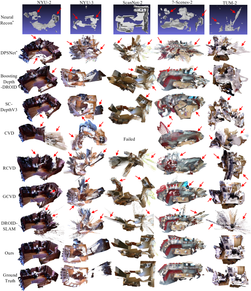
Figure S1: More qualitative comparisons of zero-shot 3D scene reconstruction. Note that NeuralRecon is trained on ScanNet[9] and can only output uncolored mesh, and ^∗ represents the employment of ground-truth camera poses during reconstruction.

Appendix J More Qualitative Comparisons

More qualitative comparisons with seven representative algorithms are shown in Fig. S1. Our method can reconstruct accurate and robust 3D scene shapes on diverse scenes.

References

- [1] Jean-Baptiste Alayrac, Jeff Donahue, Pauline Luc, Antoine Miech, Iain Barr, Yana Hasson, Karel Lenc, Arthur Mensch, Katie Millican, Malcolm Reynolds, et al. Flamingo: a visual language model for few-shot learning. Adv. Neural Inform. Process. Syst., 2022.
- [2] Paul J Besl and Neil D McKay. Method for registration of 3-d shapes. In Sensor fusion IV: control paradigms and data structures, volume 1611, pages 586–606. Spie, 1992.
- [3] Jiawang Bian, Zhichao Li, Naiyan Wang, Huangying Zhan, Chunhua Shen, Ming-Ming Cheng, and Ian Reid. Unsupervised scale-consistent depth and ego-motion learning from monocular video. Adv. Neural Inform. Process. Syst., 32, 2019.
- [4] Jia-Wang Bian, Huangying Zhan, Naiyan Wang, Tat-Jun Chin, Chunhua Shen, and Ian Reid. Auto-rectify network for unsupervised indoor depth estimation. IEEE Trans. Pattern Anal. Mach. Intell., 2021.
- [5] Fabio Bruno, Stefano Bruno, Giovanna De Sensi, Maria-Laura Luchi, Stefania Mancuso, and Maurizio Muzzupappa. From 3d reconstruction to virtual reality: A complete methodology for digital archaeological exhibition. Journal of Cultural Heritage, 11(1):42–49, 2010.
- [6] Carlos Campos, Richard Elvira, Juan J Gómez Rodríguez, José MM Montiel, and Juan D Tardós. ORB-SLAM3: An accurate open-source library for visual, visual–inertial, and multimap slam. IEEE Trans. Robotics, 37(6):1874–1890, 2021.
- [7] Kai Cheng, Hao Chen, Wei Yin, Guangkai Xu, and Xuejin Chen. Exploiting correspondences with all-pairs correlations for multi-view depth estimation. arXiv preprint arXiv:2205.02481, 2022.
- [8] Max Coenen, Franz Rottensteiner, and Christian Heipke. Precise vehicle reconstruction for autonomous driving applications. ISPRS Annals of the Photogrammetry, Remote Sensing and Spatial Information Sciences, 4:21–28, 2019.
- [9] Angela Dai, Angel X Chang, Manolis Savva, Maciej Halber, Thomas Funkhouser, and Matthias Nießner. Scannet: Richly-annotated 3d reconstructions of indoor scenes. In IEEE Conf. Comput. Vis. Pattern Recogn., pages 5828–5839, 2017.
- [10] Jakob Engel, Vladlen Koltun, and Daniel Cremers. Direct sparse odometry. IEEE Trans. Pattern Anal. Mach. Intell., 40(3):611–625, 2017.
- [11] Jakob Engel, Thomas Schöps, and Daniel Cremers. Lsd-slam: Large-scale direct monocular slam. In Eur. Conf. Comput. Vis., pages 834–849. Springer, 2014.
- [12] Christian Forster, Matia Pizzoli, and Davide Scaramuzza. Svo: Fast semi-direct monocular visual odometry. In Proc. IEEE Int. Conf. Robotics and Automation, pages 15–22. IEEE, 2014.
- [13] Andreas Geiger, Philip Lenz, Christoph Stiller, and Raquel Urtasun. Vision meets robotics: The kitti dataset. Int. J. Robotics Research, 32(11):1231–1237, 2013.
- [14] Po-Han Huang, Kevin Matzen, Johannes Kopf, Narendra Ahuja, and Jia-Bin Huang. Deepmvs: Learning multi-view stereopsis. In IEEE Conf. Comput. Vis. Pattern Recogn., pages 2821–2830, 2018.
- [15] Sunghoon Im, Hae-Gon Jeon, Stephen Lin, and In So Kweon. Dpsnet: End-to-end deep plane sweep stereo. In Int. Conf. Learn. Representations, 2018.
- [16] Johannes Kopf, Xuejian Rong, and Jia-Bin Huang. Robust consistent video depth estimation. In IEEE Conf. Comput. Vis. Pattern Recogn., pages 1611–1621, 2021.
- [17] Yao-Chih Lee, Kuan-Wei Tseng, Guan-Sheng Chen, and Chu-Song Chen. Globally consistent video depth and pose estimation with efficient test-time training. arXiv preprint arXiv:2208.02709, 2022.
- [18] Xuan Luo, Jia-Bin Huang, Richard Szeliski, Kevin Matzen, and Johannes Kopf. Consistent video depth estimation. ACM Trans. Graph., 39(4):71–1, 2020.
- [19] Raul Mur-Artal, Jose Maria Martinez Montiel, and Juan D Tardos. Orb-slam: a versatile and accurate monocular slam system. IEEE Trans. Robotics, 31(5):1147–1163, 2015.
- [20] Raul Mur-Artal and Juan D Tardós. Orb-slam2: An open-source slam system for monocular, stereo, and rgb-d cameras. IEEE Trans. Robotics, 33(5):1255–1262, 2017.
- [21] Zak Murez, Tarrence van As, James Bartolozzi, Ayan Sinha, Vijay Badrinarayanan, and Andrew Rabinovich. Atlas: End-to-end 3d scene reconstruction from posed images. In Eur. Conf. Comput. Vis., pages 414–431. Springer, 2020.
- [22] Alec Radford, Jong Wook Kim, Chris Hallacy, Aditya Ramesh, Gabriel Goh, Sandhini Agarwal, Girish Sastry, Amanda Askell, Pamela Mishkin, Jack Clark, et al. Learning transferable visual models from natural language supervision. In Int. Conf. Mach. Learn., pages 8748–8763, 2021.
- [23] René Ranftl, Alexey Bochkovskiy, and Vladlen Koltun. Vision transformers for dense prediction. In Int. Conf. Comput. Vis., pages 12179–12188, 2021.
- [24] René Ranftl, Katrin Lasinger, David Hafner, Konrad Schindler, and Vladlen Koltun. Towards robust monocular depth estimation: Mixing datasets for zero-shot cross-dataset transfer. IEEE Trans. Pattern Anal. Mach. Intell., 44(3):1623–1637, 2022.
- [25] Paul-Edouard Sarlin, Daniel DeTone, Tomasz Malisiewicz, and Andrew Rabinovich. Superglue: Learning feature matching with graph neural networks. In IEEE Conf. Comput. Vis. Pattern Recogn., pages 4938–4947, 2020.
- [26] Johannes L Schonberger and Jan-Michael Frahm. Structure-from-motion revisited. In IEEE Conf. Comput. Vis. Pattern Recogn., pages 4104–4113, 2016.
- [27] Johannes L Schönberger, Enliang Zheng, Jan-Michael Frahm, and Marc Pollefeys. Pixelwise view selection for unstructured multi-view stereo. In Eur. Conf. Comput. Vis., pages 501–518. Springer, 2016.
- [28] Jamie Shotton, Ben Glocker, Christopher Zach, Shahram Izadi, Antonio Criminisi, and Andrew Fitzgibbon. Scene coordinate regression forests for camera relocalization in rgb-d images. In IEEE Conf. Comput. Vis. Pattern Recogn., pages 2930–2937, 2013.
- [29] Nathan Silberman, Derek Hoiem, Pushmeet Kohli, and Rob Fergus. Indoor segmentation and support inference from rgbd images. In Eur. Conf. Comput. Vis., pages 746–760. Springer, 2012.
- [30] Jürgen Sturm, Nikolas Engelhard, Felix Endres, Wolfram Burgard, and Daniel Cremers. A benchmark for the evaluation of rgb-d slam systems. In IEEE/RSJ Int. Conf. Intelligent Robots and Systems, pages 573–580, 2012.
- [31] Jiaming Sun, Yiming Xie, Linghao Chen, Xiaowei Zhou, and Hujun Bao. Neuralrecon: Real-time coherent 3d reconstruction from monocular video. In IEEE Conf. Comput. Vis. Pattern Recogn., pages 15598–15607, 2021.
- [32] Libo Sun, Jia-Wang Bian, Huangying Zhan, Wei Yin, Ian Reid, and Chunhua Shen. Sc-depthv3: Robust self-supervised monocular depth estimation for dynamic scenes. arXiv preprint arXiv:2211.03660, 2022.
- [33] Wei Sun, Binil Starly, Jae Nam, and Andrew Darling. Bio-cad modeling and its applications in computer-aided tissue engineering. Computer-aided design, 37(11):1097–1114, 2005.
- [34] Zachary Teed and Jia Deng. Raft: Recurrent all-pairs field transforms for optical flow. In Eur. Conf. Comput. Vis., pages 402–419. Springer, 2020.
- [35] Zachary Teed and Jia Deng. Droid-slam: Deep visual slam for monocular, stereo, and rgb-d cameras. Adv. Neural Inform. Process. Syst., 34:16558–16569, 2021.
- [36] Bill Triggs, Philip McLauchlan, Richard Hartley, and Andrew Fitzgibbon. Bundle adjustment—a modern synthesis. In International Workshop on Vision Algorithms, pages 298–372, 1999.
- [37] Enze Xie, Wenhai Wang, Zhiding Yu, Anima Anandkumar, Jose M Alvarez, and Ping Luo. Segformer: Simple and efficient design for semantic segmentation with transformers. Advances in Neural Information Processing Systems, 34:12077–12090, 2021.
- [38] Yiming Xie, Matheus Gadelha, Fengting Yang, Xiaowei Zhou, and Huaizu Jiang. Planarrecon: Real-time 3d plane detection and reconstruction from posed monocular videos. In IEEE Conf. Comput. Vis. Pattern Recogn., pages 6219–6228, 2022.
- [39] Guangkai Xu, Wei Yin, Hao Chen, Chunhua Shen, Kai Cheng, Feng Wu, and Feng Zhao. Towards 3d scene reconstruction from locally scale-aligned monocular video depth. arXiv preprint arXiv:2202.01470, 2022.
- [40] Ming-Der Yang, Chih-Fan Chao, Kai-Siang Huang, Liang-You Lu, and Yi-Ping Chen. Image-based 3d scene reconstruction and exploration in augmented reality. Automation in Construction, 33:48–60, 2013.
- [41] Yao Yao, Zixin Luo, Shiwei Li, Tian Fang, and Long Quan. Mvsnet: Depth inference for unstructured multi-view stereo. In Eur. Conf. Comput. Vis., pages 767–783, 2018.
- [42] Wei Yin, Yifan Liu, and Chunhua Shen. Virtual normal: Enforcing geometric constraints for accurate and robust depth prediction. IEEE Trans. Pattern Anal. Mach. Intell., 2021.
- [43] Wei Yin, Jianming Zhang, Oliver Wang, Simon Niklaus, Simon Chen, Yifan Liu, and Chunhua Shen. Towards accurate reconstruction of 3d scene shape from a single monocular image. IEEE Trans. Pattern Anal. Mach. Intell., pages 1–21, 2022.
- [44] Wei Yin, Jianming Zhang, Oliver Wang, Simon Niklaus, Long Mai, Simon Chen, and Chunhua Shen. Learning to recover 3d scene shape from a single image. In IEEE Conf. Comput. Vis. Pattern Recogn., pages 204–213, 2021.
- [45] Andy Zeng, Shuran Song, Matthias Nießner, Matthew Fisher, Jianxiong Xiao, and Thomas Funkhouser. 3dmatch: Learning local geometric descriptors from rgb-d reconstructions. In IEEE Conf. Comput. Vis. Pattern Recogn., pages 1802–1811, 2017.
- [46] Tinghui Zhou, Matthew Brown, Noah Snavely, and David G Lowe. Unsupervised learning of depth and ego-motion from video. In IEEE Conf. Comput. Vis. Pattern Recogn., pages 1851–1858, 2017.