Optimizing Performance of Feedforward and Convolutional Neural Networks through Dynamic Activation Functions

Abstract

Deep learning training training algorithms are a huge success in recent years in many fields including speech, text,image video etc. Deeper and deeper layers are proposed with huge success with resnet structures having around 152 layers. Shallow convolution neural networks(CNN’s) are still an active research, where some phenomena are still unexplained. Activation functions used in the network are of utmost importance, as they provide non linearity to the networks. Relu’s are the most commonly used activation function.We show a complex piece-wise linear(PWL) activation in the hidden layer. We show that these PWL activations work much better than relu activations in our networks for convolution neural networks and multilayer perceptrons. Result comparison in PyTorch for shallow and deep CNNs are given to further strengthen our case.

Keywords activation function, non-linearity, piecewise linear

1 Introduction

In recent years, deep learning architectures have found tremendous success in speech recognition, image recognition, language recognition and translation. For speech, languague recognition and translation, deep recurrent neural networks(RNNs)[1][2][3] have shown improvements over older technologies. These networks can not only process images but also can process sequences of images such as videos, text and speech. The RNN structure consists of cells and gates. These cells store important information over time and the gates decide the passage of information in and out of the cells. RNNs are faced with vanishing gradient problems and cannot process words over a long period of time. To address this situation, networks such as long shot term memory(LSTM)[4], gated recurrent unit(GRU)[5] and transformers[6] are shown. These networks are designed to handle long sequences over time and are also used for image processing. Convolutional Neural networks(CNNs)([7], [8], [9]) are more widely used in image based applications. Combination networks such as CNN-LSTM, CNN-transfomer are also used for visual recognition[10][11] and time series analysis[12]

CNNs are used for image based application as a feature extractor, where one doesnt need to explicitly extract features for classifying images. Applications for CNNs include in diabetic retinopathy screening[13], lesion detection[14][15], skin lesion classification[16], human action recognition[17] [18], face recognition [19] [20], document analysis[21] [22] and in many other applications. CNNs can be trained using gradient approaches such as back propagation ([23], [24], [25], [26]), and conjugate gradient ([27],[28],[29], [30]).

Despite their popularity, CNNs still have some limitations such as its poorly understood shift - invariance, overfitting of the data, and the use of oversimplified nonlinear activation functions such as relu [31],and leaky relu [32][33].

Nonlinear activation functions such as relu[31] and leaky relu [32] have been widely used in a number of computer vision[34] and deep neural network[35] applications. These activation functions are not as complex as sigmoids [36] or hyperbolic tangent functions(tanh)[37] but are favored because they partially solve the vanishing gradient problem [38]. These relu activations do not guarantee optimal results as different sets of activations can lead to optimal results for each of the filters. For example. A CNN for a image classication application with 20 filters might need 20 different activations. The number of filters required for a particular application is not known.

Although, these activations lead to universal approximation[39] in mutlilayer perceptrons, many attempts have been made to create adaptive or fixed piecewise linear activation function [[40], [41], [42] ,[43] ,[44]]. Adaptive activation functions for deep CNNs are introduced in[45], where the author trains the slope and hinges on the curve using gradient descent techniques. The author has shown promising results in terms of testing accuracies in CIFAR-10 and CIFAR-100 image recognition dataset[46] and high-energy physics involving Higgs boson decay modes[47].

In this paper, we first briefly review the multilayer perceptron’s (MLP’s) architecture, notation, training and its properties. In section II, we review the CNN architecture and notation as well as its back propagation algorithm. In Section III, we investigate a trainable piecewise linear (PWL) activation, since they can approximate the optimal mix of activations through universal approximation. In section IV, we compare our results with relu activations. Finally, In Section VII, we discuss additional work and conclude this dissertation.

2 Prior Work

In this section, we review our notation for a single hidden layer cascade connected MLP, briefly summarize several commonly used feedforward classifier training methods and describe some of the MLP’s properties.

2.1 MLP Structure and notation

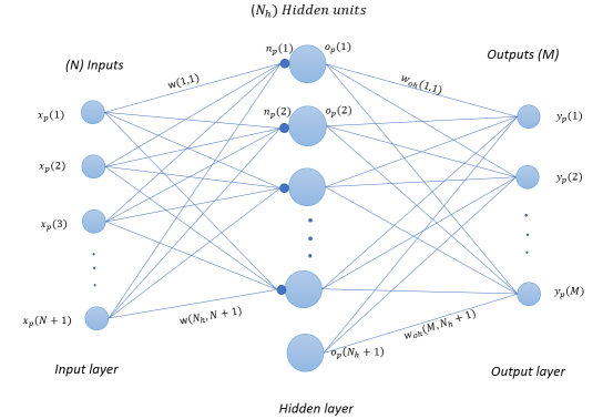
Figure 1: Single Hidden Layer MLP

A cascade connected MLP with one hidden layer is shown in figure 1. Input weight $w(k,n)$ connects the $n^{th}$ input to the $k^{th}$ hidden unit. Output weight $w_{oh}(i,k)$ connects the $k^{th}$ hidden unit’s activation $o_{p}(k)$ to the $i^{th}$ output. $y_{p}(i)$ is the $p^{th}$ pattern, $i^{th}$ output activation which is linear activation in figure1. In the training pattern $\{\mathbf{x}_{p}$, $\mathbf{t}_{p}\}$ for a MLP, the $p^{th}$ input vector $\mathbf{x}_{p}$ is initially of dimension N and the $p^{th}$ desired output (target) vector $\mathbf{t}_{p}$ has dimension M. The pattern number p varies from 1 to $N_{v}$. The threshold is handled by augmenting $\mathbf{x}_{p}$ with an extra element $X_{p}(n+1)$ which is equal to one where, $\mathbf{x}_{p}$ = $[x_{p}(1),x_{p}(2),....,x_{p}(N+1)]^{T}$

For the $p^{th}$ pattern, the $k^{th}$ hidden unit’s net function $n_{p}(k)$ is then

$$n_{p}(k)=\sum_{n=1}^{N+1}w(k,n)\cdot x_{p}(n)$$ (1)

which can be summarized as

$$\mathbf{n}_{p}=\mathbf{W}\cdot\mathbf{x}_{p}$$ (2)

where $\mathbf{n}_{p}$ denotes the $N_{h}$ dimensional column vector of net function values and the input weight matrix $\mathbf{W}$ is $N_{h}$ by (N+1). For the $p^{th}$ pattern, the $k^{th}$ hidden unit’s output, $o_{p}(k)$, is given as

$$o_{p}(k)=f(n_{p}(k))$$ (3)

where $f(.)$ denotes a nonlinear hidden layer activation function, such as relu[31] which is represented as

$$f(n_{p}(k))=\begin{cases}n_{p}(k),\quad if\quad n_{p}(k)\geq 0\\ 0,\quad if\quad n_{p}(k)<0\\ \end{cases}$$ (4)

The threshold in the hidden layer is handled by augmenting $\mathbf{o}_{p}$ with an extra element $o_{p}(N_{h}+1)$ which is equal to one where $\mathbf{o}_{p}$ = $[o_{p}(1),o_{p}(2),....,o_{p}(N_{h}+1)]^{T}$. The network’s output vector for the $p^{th}$ pattern is $\mathbf{n}_{po}$. The $i^{th}$ element $n_{po}(i)$ of the M-dimensional output vector $\mathbf{n}_{po}$ is

$$n_{po}(i)=\sum_{k=1}^{N_{h}+1}w_{o}(i,k)\cdot o_{p}(k)$$ (5)

which can be summarized as

$$\mathbf{N}_{po}={\mathbf{W}_{o}}\cdot\mathbf{o}_{p}$$ (6)

$\mathbf{W_{o}}$ is the output weight matrix with dimensions $M$ by ($N_{h}+1$).

The output layer net vector $\textbf{n}_{po}$ is passed through an activation function for $i^{th}$ output which is given in terms of $p^{th}$ pattern and $i^{th}$ output, $y_{p}(i)$ as,

$$y_{p}(i)=f_{o}(\textbf{n}_{po}(i))$$ (7)

where $f_{o}(.)$ denotes a output hidden layer activation function. The most commonly used activation function for approximation data is the linear activation, sigmoid activation is mostly used in logistic regression and softmax activation [48] is used for classification models which is defined in equation (8).

The softmax output activation function is

$$y_{p}(i)=\frac{exp(n_{po}(i))}{\sum_{k=1}^{M}exp(n_{po}(k))}$$ (8)

The most commonly used objective function for a classification task is cross entropy loss function[48]

$$E_{ce}=\frac{1}{N_{v}}\sum_{p=1}^{N_{v}}[-\sum_{i=1}^{M}t_{p}(i)\cdot log(y_{p}(i))]$$ (9)

where $t_{p}(i)$ is the $p^{th}$ pattern and $i^{th}$ class one hot encoded output. $t_{p}(i)$ is found from $ic_{p}(i)$, where $ic_{p}(i)$ is the class number. For approximation or regression, mean square error(MSE)[49] defined in equation (10) is the most widely used objective function. The MSE can also be used in the classification task with output reset[50][51].

$$E=\frac{1}{N_{v}}\sum_{p=1}^{N_{v}}\sum_{i=1}^{M}[t_{p}(i)-y_{p}(i)]^{2}$$ (10)

2.2 CNN structure and notation

In this section, we first review notation and training of a convolutional neural network with a single convolution layer. Then we extend the notation to cover CNNs with multiple hidden layers.

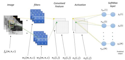
Figure 2: Shallow CNN with Linear softmax cross-entropy classifier

The CNN network structure is shown in figure 2. Let ${\mathbf{f}_{p}}$ denote the $p^{th}$ input image and let $i_{c}(p)$ denote the correct class number of the $p^{th}$ pattern, where $p$ varies from $1$ to $N_{v}$, and $N_{v}$ is the total number of training images or patterns.

During forward propagation, a filter of size $N_{f}$ x $N_{f}$ is convolved over the image $f_{1}$ with $N_{r}$ rows, $N_{c}$ columns.The number of channels is denoted by $C$, where color input images have $C$ equal to $3$ and grayscale images have $C$ equal to $1$.

For the $k^{th}$ filter, the net function output for the $i^{th}$ row and $j^{th}$ column is

$$n_{p}(k,i,j)=t_{r}(k)+\sum_{m=1}^{N_{f}}\sum_{n=1}^{N_{f}}\sum_{c=1}^{C}w_{f}(k,m,n,c)\cdot f_{p}(m+(i-1)s,n+(j-1)s,c)$$ (11)

where, $\mathbf{n}_{p}$ is of size ($K$ by $M_{o}$ by $N_{o}$), where $K$ is the number of filters, $M_{o}$ is the height of the convolved image output and $N_{o}$ is the width of the convolved image output. $w_{f}(k,m,n,c)$ is the filter of size ($K$ by $N_{f}$ by $N_{f}$ by $C$). The threshold vector $\mathbf{t_{r}}$ is added to the net function output as shown in equation (11). The stride $s$ is the number of filter shifts over input images. Note that the output $n_{p}(k,i,j)$ in 11 us a threshold plus a sum of $C$ separate 2-D convolution, rather than a 3-D convolution.

To achieve non-linearity, the convolved image with element $n_{p}(k,i,j)$ is passed through a relu activation [31] as

$$o_{p}(k,i,j)=f^{\prime}(n_{p}(k,i,j))$$ (12)

where, $o_{p}(k,i,j)$ is the $k^{th}$ filter’s hidden unit activation output for the $i^{th}$ row, $j^{th}$ column for the $p^{th}$ pattern of size ($K$ by $N_{rb}$ by $N_{cb}$), where $N_{rb}$ by $N_{cb}$ is the row and column size of the output of the convolved image respectively.

The net function $\mathbf{n}_{po}$ for $i^{th}$ element of the CNN’s output layer for the $p^{th}$ pattern is

$$n_{po}(i)=t_{o}(i)+\sum_{m=1}^{M_{o}}\sum_{n=1}^{N_{o}}\sum_{k=1}^{K}w_{o}(i,m,n,k)\cdot o_{p}(k,m,n)$$ (13)

where $\mathbf{W_{o}}$ is the 4 dimensional matrix of size ($M$ by $M_{o}$ by $N_{o}$ by $K$), which connects hidden unit activation outputs or features to the output layer net vector $\mathbf{n}_{po}$, $\mathbf{o}_{p}$ is a 3 dimensional hidden unit activation output matrix of size ($M_{o}\cdot N_{o}\cdot K$) and $\mathbf{t_{o}}$ is the vector of biases added to net output function as in equation (13).

Before calculating the final error, the vector $\mathbf{n}_{po}$ is passed through an activation function such as softmax in 8. Finally the cross entropy loss function is calculated using equation 9. The objective function is reduced with respect to the unknown weights. In this chapter, we discuss CNN training of classification models. We minimise the loss function $E_{ce}$ using steepest descent [52][53][54], [55][56]. The most common optimizer used for CNN weight training is using Adams optimizer [57]. It is computationally efficient and easier to implement than optimal learning factor [58]. It uses momentum and adaptive learning rates to converge faster, which is said to be inherited from RMSProp[59] and AdaGrad[60]. The default parameters are given in [57].

3 Training algorithm

3.1 Scaled conjugate gradient algorithm

Conjugate gradient (CG) [61] line-searches in successive conjugate directions and has faster convergence than steepest descent. To train an MLP using the CG algorithm (CG-MLP), we update all the network weights $\mathbf{w}$ simultaneously as follows:

$$\mathbf{w}\leftarrow\mathbf{w}+z\cdot\mathbf{p}\\$$ (14)

where $z$ is the learning rate that can be derived as [62],[61].

$$z=-{\frac{\frac{\partial E(\mathbf{w}+z\cdot\mathbf{p})}{\partial z}}{\frac{\partial^{2}E(\mathbf{w}+z\cdot\mathbf{p})}{\partial z^{2}}}}|_{z=0}$$ (15)

The direction vector $\mathbf{p}$ is obtained from the gradient $\mathbf{g}$ as

$$\mathbf{p}\leftarrow-\mathbf{g}+B_{1}\cdot\mathbf{p}$$ (16)

where $\mathbf{p}$ = $vec$ $(\mathbf{P},\mathbf{P}_{\textrm{oh}},\mathbf{P}_{\textrm{oi}})$ and $\mathbf{P}$, $\mathbf{P}_{\textrm{oh}}$ and $\mathbf{P}_{\textrm{oi}}$ are the direction vectors corresponding to weight arrays $(\mathbf{W},\mathbf{W}_{\textrm{oh}},\mathbf{W}_{\textrm{oi}})$. CG uses backpropagation to calculate $\mathbf{g}$. $B_{1}$ is the ratio of the gradient energy from two consecutive iterations. If the error function were quadratic, CG would converge in $N_{w}$ iterations [63], where the number of network weights is $N_{w}$ = $dim(\mathbf{w})$. CG is scalable and widely used in training large datasets, as the network Hessian is not calculated [64]. Therefore, in a CG, the step size is determined using a line search along the direction of the conjugate gradient.

SCG [65] scales the conjugate gradient direction by a scaling factor determined using a quasi-Newton approximation of the Hessian matrix. This scaling factor helps to accelerate the algorithm’s convergence, especially for problems where the condition number of the Hessian matrix is large. SCG requires the computation of the Hessian matrix (or an approximation) and its inverse. A critical difference between CG and SCG is how the step size is determined during each iteration, with SCG using a scaling factor that helps to accelerate convergence. Other variations of CG exist [66]. However, in this study, we choose to use SCG.

3.2 Levenberg-Marquardt algorithm

The Levenberg-Marquardt (LM) algorithm [61] is a hybrid first- and second-order training method that combines the fast convergence of the steepest descent method with the precise optimization of the Newton method [67]. However, inverting the Hessian matrix $\mathbf{H}$ can be challenging due to its potential singularity or ill-conditioning [68]. To address this issue, the LM algorithm introduces a damping parameter $\lambda$ to the diagonal of the Hessian matrix as

$$\mathbf{H}_{LM}=\mathbf{H}+\lambda\cdot\mathbf{I}$$ (17)

where $\mathbf{I}$ is an identity matrix with dimensions equal to those of $\mathbf{H}$. The resulting matrix $\mathbf{H}_{LM}$ is then nonsingular, and the direction vector $\mathbf{d}_{LM}$ can be calculated by solving:

$$\mathbf{H}_{LM}\mathbf{d}_{LM}=\mathbf{g}$$ (18)

The constant $\lambda$ represents a trade-off value between first and second order for the LM algorithm. When $\lambda$ is close to zero, LM approximates Newton’s method and has minimal impact on the Hessian matrix. When $\lambda$ is large, LM approaches the steepest descent and the Hessian matrix approximates an identity matrix. However, the disadvantage of the LM algorithm is that it scales poorly and is only suitable for small data sets [61].

3.3 Basic MOLF

In basic MOLF MLP training [69], the input weight matrix $\mathbf{W}$ is initialized randomly using zero-mean Gaussian random numbers. To initialize the output weight matrix $\mathbf{W}_{\textrm{o}}$, we use output weight optimization (OWO) [61]. OWO minimizes the error function from equation (10) with respect to $\mathbf{W}_{\textrm{o}}$ by solving the $M$ sets of $N_{u}$ equations in $N_{u}$ unknowns given by

$$\mathbf{C}=\mathbf{R\cdot W_{o}^{T}}$$ (19)

where the cross-correlation matrix $\mathbf{C}$ and the auto-correlation matrix $\mathbf{R}$ are respectively

$$\mathbf{C}=\frac{1}{N_{v}}\sum_{p=1}^{N_{v}}\mathbf{X}_{\textrm{ap}}\cdot\mathbf{t}_{\textrm{p}}^{T}$$ (20)

$$\mathbf{R}=\frac{1}{N_{v}}\sum_{p=1}^{N_{v}}\mathbf{X}_{\textrm{ap}}\cdot\mathbf{X}_{\textrm{ap}}^{T}$$ (21)

In terms of optimization theory, solving equation (19) is merely Newton’s algorithm for the output weights [61]. After initialization of $\mathbf{W}$ , $\mathbf{W}_{\textrm{oi}}$, $\mathbf{W}_{\textrm{oh}}$, we begin a two step procedure in which we modify $\mathbf{W}$ and perform OWO to modify $\mathbf{W}_{\textrm{o}}$. In the $\mathbf{W}$ modification step we first find the input weight negative gradient matrix $\mathbf{G}$ and solve

$$\mathbf{D}\cdot\mathbf{R}_{\textrm{i}}=\mathbf{G}$$ (22)

for $\mathbf{D}$, where

$$\mathbf{R}_{\textrm{i}}=\frac{1}{N_{v}}\sum_{p=1}^{N_{v}}\mathbf{x}_{\textrm{ap}}\cdot\mathbf{x}_{\textrm{ap}}^{T}$$ (23)

It has been shown [61] that the improved input weight change matrix $\mathbf{D}$ is the negative gradient matrix that results when the inputs are whitened. In MOLF, the idea is to use an $N_{h}$ dimensional learning factor vector $\mathbf{z}$ and to write the updated ouputs as

$$y_{p}(i)=\sum_{n=1}^{N+1}w_{oi}(i,n)x_{p}(n)+\sum_{k=1}^{N_{h}}w_{oh}(i,k)f(n_{p}(k))$$ (24)

$$n_{p}(k)=\sum_{n=1}^{N+1}(w(k,n)+z_{k}d(k,n)x_{p}(n))$$

where, $d(k,n)$ is an element of the matrix $\mathbf{D}$. We use Newton’s method to obtain $\mathbf{z}$ by solving

$$\mathbf{H}_{\textrm{molf}}\cdot\mathbf{z}=\mathbf{g}_{\textrm{molf}}$$ (25)

where $\mathbf{H}_{\textrm{molf}}$ and $\mathbf{g}_{\textrm{molf}}$ are the Hessian and negative gradient, respectively, of the error with respect to $\mathbf{z}$. Our implementation of Newton’s method solves equation (25) for $\mathbf{z}$ using orthogonal least squares (OLS) [61]. After finding $\mathbf{z}$, we update the input weight matrix $\mathbf{W}$ as

$$\mathbf{W}\leftarrow\mathbf{W}+diag(\mathbf{z})\cdot\mathbf{D}$$ (26)

The MOLF training algorothm (MA algorithm) [55] is as given in algorithm 1.

Algorithm 1 MA algorithm

1:Read the training data.

2:Randomly split off 30 % data of the training data to be validation data.

3:Initialize $N_{it}^{3}$ , $i_{t}$ $\leftarrow$ 0, $\mathbf{C}$ $\leftarrow$ 0 , $N_{h}$ and network weights.

4:Calculate $\mathbf{R}$ and $\mathbf{C}$ using equation (20).

5:Solve equation (19) for the initial output weight matrix $\mathbf{W}_{\textrm{o}}$.

6:while $i_{t}$ $<$ $N_{it}^{3}$ do

7:     BP step : Compute the negative input weight gradient matrix $\mathbf{G}$ and solve for $\mathbf{D}$ using equation (22)

8:     MOLF step : Solve equation (25) for $\mathbf{z}$ using OLS

9:     Update $\mathbf{W}$ as $\mathbf{W}$ $\leftarrow$ $\mathbf{W}$ + diag($\mathbf{z}$) $\cdot$ $\mathbf{D}$

10:     OWO step : Solve equation (19) to obtain $\mathbf{W}_{\textrm{o}}$

11:     Save $\mathbf{W}$ and $o(n)$ if validation error has decreased.

12:     $i_{t}$ $\leftarrow$ $i_{t}$ + 1

13:end while

3.4 Modifying targets with output reset

The MA algorithm of subsection 3.1 is a first attempt at attacking problems (P4) and (P5) in approximation networks. In this subsection, we adapt MA to classification networks. Problem (P1) is attacked by developing new target outputs $t_{p}^{{}^{\prime}}(i)$, while keeping the constraint that the target margin satisfies $t_{p}^{{}^{\prime}}(i_{c})$ - $t_{p}^{{}^{\prime}}(i_{d}$) $\geq$ 1. There are two kinds of inconsistent errors which simultaneously increase E and decrease $P_{e}$ or leave $P_{e}$ the same. First each pattern’s output $\mathbf{y}_{p}$ can have a bias so that the average of $t_{p}(i)$ over $i$, differs from the average of $y_{p}(i)$. Second, as stated in problem (P1), we can have $y_{p}(i_{c})$ $>$ $t_{p}(i_{c})$ or $y_{p}(i_{d})$ $<$ $t_{p}(i_{d})$. In order to remove these inconsistent errors we design a new error function $E^{{}^{\prime}}$ [69] in which targets, but not labels are changed [70].

$${E^{{}^{\prime}}=\frac{1}{N_{v}}\sum_{p=1}^{Nv}\sum_{i=1}^{M}[t^{{}^{\prime}}_{p}(i)-y_{p}(i)]^{2}}$$ (27)

where $t_{p}^{{}^{\prime}}(i)$ is modeled as

$$t^{{}^{\prime}}_{p}(i)=t_{p}(i)+a_{p}+d_{p}(i)$$ (28)

and where $a_{p}$ and $d_{p}(i)$ are initially equal to zero. Since $a_{p}$ is the same for each class, it has no effect on $P_{e}$. Following [69], we calculate the closed form expression for $a_{p}$ by setting $\frac{\partial E^{{}^{\prime}}}{\partial a_{p}}$ = 0, therefore obtaining

$$a_{p}=\frac{1}{M}\sum_{i=1}^{M}[y_{p}(i)-t_{p}^{{}^{\prime}}(i)-d_{p}(i)]$$ (29)

Similarly, $d_{p}(i)$ is defined as

$$d_{p}(i)=y_{p}(i)-t_{p}^{{}^{\prime}}(i)-a_{p}$$ (30)

such that $d_{p}(i_{c})$ $\geq$ 0 and $d_{p}(i_{d})$ $\leq$ 0. It is true that $a_{p}$ and $d_{p}(i)$ can be included in $t_{p}^{{}^{\prime}}(i)$ or $y_{p}(i)$ during training. However, these parameters are not available during testing because they make use of the correct class $i_{c}(p)$, which is unknown. Therefore we include them in $t_{p}^{{}^{\prime}}(i)$.

To avoid inconsistent errors we need $t_{p}^{{}^{\prime}}(i_{c})$ $\geq$ $y_{p}(i_{c})$ and $t_{p}^{{}^{\prime}}(i_{d})$ $\leq$ $y_{p}(i_{d})$ so

$$d_{p}(i_{c})=[y_{p}(i_{c})-a_{p}-t_{p}(i_{c})]u(y_{p}(i_{c})-a_{p}-t_{p}(i_{c}))$$ (31)

and

$$d_{p}(i_{d})=[y_{p}(i_{d})-a_{p}-t_{p}(i_{d})]u(t_{p}(i_{d})-a_{p}-y_{p}(i_{d}))$$ (32)

where u($\cdot$) denotes the unit step function. Note here that for a classifier, the training halts when $E^{{}^{\prime}}$ becomes zero, even if $E$ is nonzero. The effect of (P2) is reduced because

$$\lim_{y_{p}(i_{c})\to\infty}(y_{p}^{{}^{\prime}}(i_{c})-t_{p}(i_{c}))=0$$ (33)

and similarly

$$\lim_{y_{p}(i_{d})\to-\infty}(y_{p}^{{}^{\prime}}(i_{d})-t_{p}(i_{d}))=0$$ (34)

We denote the process of obtaining $t_{p}^{{}^{\prime}}$ as an output reset (OR) algorithm and describe it as follows

Algorithm 2 OR algorithm

Given $p$, $t_{p}(i)$ and $y_{p}(i)$ from the current regression based classifier, initialize $a_{p}$ to zero and $d_{p}(i)$ to zero for 1 $\leq$ i $\leq$ M.

for $i_{t}$ = 1 to 3 do

     Calculate $a_{p}$ using (29).

     for $i$ = 1 to M do

         Calculate $d_{p}(i)$ using (31) and (32)

         Calculate $t_{p}^{{}^{\prime}}(i)$ using (28)

     end for

end for

Note that in algorithm 2, letting the maximum number of iterations equal 3 allows considerable improvement in performance without a significant change in training time [69]. In [69], the heuristic iterative OR algorithm is replaced by an efficient closed form expression for the target outputs. In other words, the OR algorithm is a multi-class version of Ho-Kashyap [69]. By adding OR to the MA algorithm, we generate MA-OR. The MA-OR algorithm can be summarized as follows:

Algorithm 3 MA-OR algorithm

1:Read the training data.

2:Randomly split off 30 % data of the training data to be validation data.

3:Initialize $N_{it}^{3}$ , $i_{t}$ $\leftarrow$ 0, $\mathbf{C}$ $\leftarrow$ 0 , $N_{h}$ and network weights.

4:Calculate $\mathbf{R}$ and $\mathbf{C}$ using equation (20).

5:Solve equation (19) for the initial output weight matrix $\mathbf{W}_{\textrm{o}}$.

6:while $i_{t}$ $<$ $N_{it}^{3}$ do

7:     BP step : Compute $\mathbf{G}$ using $t^{{}^{\prime}}_{p}(i)$ from OR instead of $t_{p}(i)$, and solve for $\mathbf{D}$ using equation (22)

8:     MOLF step : Solve equation (25) for $\mathbf{z}$ using OLS

9:     Update $\mathbf{W}$ as $\mathbf{W}$ $\leftarrow$ $\mathbf{W}$ + diag($\mathbf{z}$) $\cdot$ $\mathbf{D}$

10:     OWO step : Accumulate $\mathbf{C}$ using $t^{{}^{\prime}}_{p}(i)$ in-place of $t_{p}(i)$. Solve equation (19) to obtain $\mathbf{W}_{\textrm{o}}$

11:     Save $\mathbf{W}$ and $o(n)$ if validation error has decreased.

12:     $i_{t}$ $\leftarrow$ $i_{t}$ + 1

13:end while

3.5 Softmax classifier

The softmax classifier [61] is a generalized logistic regression classifier that outputs approximate class probabilities. Structurally, it’s a linear model with softmax functions [71] at the output units. For the $p^{th}$ pattern, it maps the input vector $\mathbf{x}_{\textrm{p}}$ to the output class labels as

$$\mathbf{y}_{\textrm{p}}=\mathbf{W}_{\textrm{s}}\cdot\mathbf{x}_{\textrm{p}}$$ (35)

where $\mathbf{W}_{\textrm{s}}$ is a weight matrix. The performance measure is a cross-entropy loss function [61] defined as

$$E_{softmax}=-\frac{1}{N_{v}}\sum_{p=1}^{N_{v}}\sum_{i=1}^{M}log(\frac{e^{y_{p}(i)}}{\sum_{j=1}^{M}e^{y_{p}(j)}})$$ (36)

The softmax classifier is often trained using the L-BFGS training algorithm[61].

3.6 Fixed Activation function

3.7 Piecewise Linear Unit(PLU) Activation

PWL functions are composed of Relu activations [35]. Activations such as sigmoid[36] and tanh[37] can be approximated using relu units. Several investigators have tried adaptive PWL activation functions in MLPs[41] and deep learning[45] and have published promising results. One of them includes hybrid piecewise linear units(PLU) with an activation function that is a combination of tanh and relu activations[40].

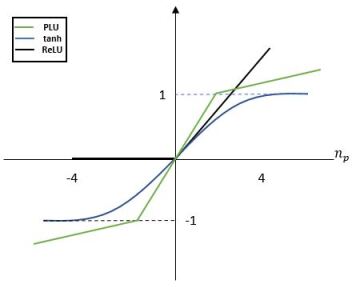
Figure 3: Fixed PWL activations

From figure 3, we see that PLU is a combination of relu and tanh activations. The equation for calculating fixed PWL activations is given as

$$o_{p}(k)=max\left[\alpha(n_{p}(k)+c)-c,min(\alpha(n_{p}(k)+c)-c,n_{p}(k))\right]$$ (37)

where, $\alpha$ and $c$ are user chosen parameters. The author has also proposed that the $\alpha$ can also be a trainable parameter. The paper [40] demonstrates the performance of fixed PWL in an MLP for paramteric functions, 3D surface approximation and invertible network datasets. The author shows that fixed PLUs work better than relu functions as PLUs are represented using more hinges than relu functions. The author also shown promising results using CNN for the cifar 10[46] dataset. The fixed PWL activation function has only 3 linear segments, hinges $H$ = 3 and will not be adaptive until the $\alpha$ parameter is trained in every iteration. Since the $H$ is fixed and there is minimal or no training , there is no universal approximation.

3.8 Piecewise Linear Activation

An alternate piecewise linear activation has been demonstrated[45], which is specifically designed for deep networks with trainable PWL activations. This method therefore outperforms the fixed PWL activation in section 3.7. The adaptive PWL activations here can equal those of section 3.7 and can also generate more complicated curves. The author has implemented an adaptive piecewise linear activation unit where the number of hinges $H$ is a hyperparameter that is user chosen. The author shows the best results for CIFAR10 data using $H=5$ and $H=2$, and for CIFAR100 data using $H=2$ and $H=1$(no activation hinge training). The initialization for there adaptive activations is not properly specified.

The equation for calculating the the adaptive activation is given as

$$o_{p}(k)=max(0,n_{p}(k))+\sum_{s=1}^{H}a_{k}^{s}\cdot max(0,-n_{p}(k)+b_{k}^{s})$$ (38)

where, $a_{i}^{s}$ and $b_{i}^{s}$ for $i=1..H$ are learned using gradient descent. $a_{i}$ variables control the slopes of the linear segments and $b_{i}^{s}$ determine the locations of sample points.

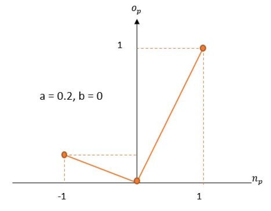
Figure 4: 2 relu curves

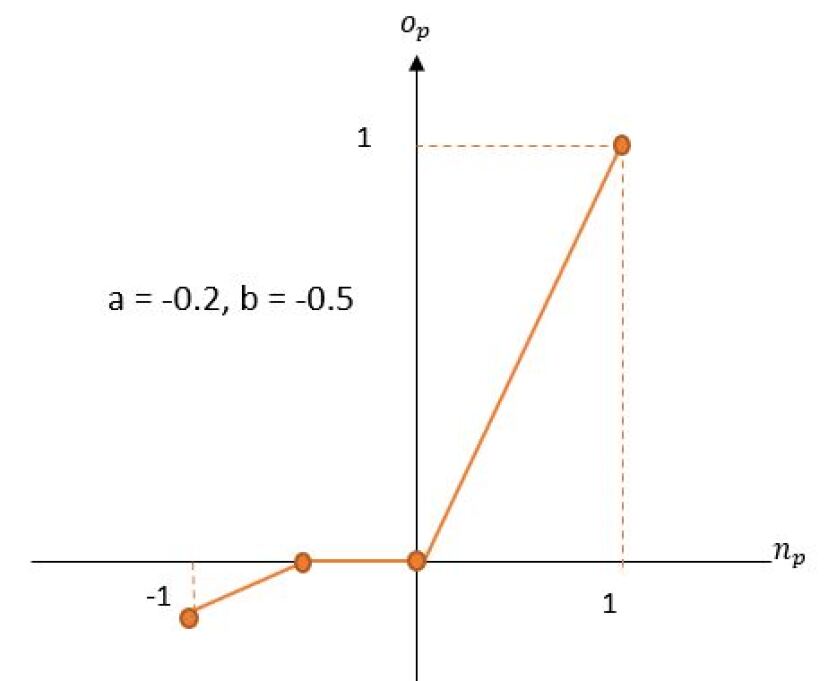
Figure 5: 4 relu curves

figure 5 shows adaptive PWL with slope $a$ as 0.2 and $b$ as 0. Similarly, figure 5 shows adaptive PWL with slope $a$ as -0.2 and $b$ as -0.5.

4 Proposed work

4.1 Mathematical Background

Section 3.8 describes an adaptive PWL activation which trains the locations and slopes of the hinges. The author claims that a small number of hinges achieved better results. We see in section 3.7 that a network with two hinges outperforms relu for a particular application. To approximate a linear output, only one hinge is needed on the PWL curve. Similarly, to approximate a quadratic output, the number of hinge sets on the PWL curve should be larger than three. Therefore, the number of hinges should not be less for more complicated datasets. This can also result in using fewer hidden layers and filters as the network doesn’t need to train for a longer time.

We further investigate the use of PWL activations in CNNs[72] and we first determine that PWL activations can approximate any other existing activation functions. Consider a CNN filter’s net function $n_{1}$ defined as

$$n_{1}=t+\sum_{m=1}^{N}w_{i}(m)\cdot x(m)$$ (39)

where t is the threshold, $w_{i}(m)$ is the $m^{th}$ filter weight, and $x(m)$ is the $m^{th}$ input to the net function. The filter can be represented as $\{\mathbf{w_{i}},t\}$. The continuous PWL activation $f(n_{1})$ is

$$f(n_{1})=\sum_{k=1}^{N_{s}}a_{k}\cdot r(n_{1}-ns_{k})$$ (40)

where $N_{s}$ denotes the number of segments in the PWL curve, $r()$ denotes a ramp (relu) activation, and $ns_{k}$ is the net function value at which the $k^{th}$ ramp switches on.

Figure 6: Approximate sigmoid using 2 relu curves

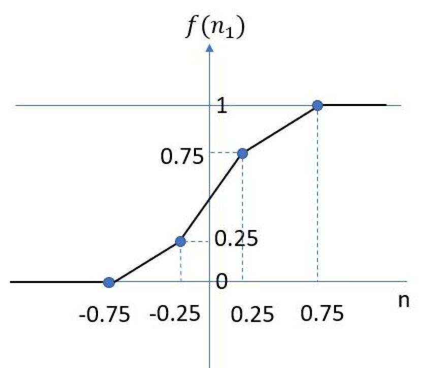
Figure 7: Approximate sigmoid using 4 relu curves

Figures 7 and 7 show approximate sigmoid curves generated using relu activations where figure 7 has $N_{s}$ = $2$ relu curves and figure 7 has $N_{s}$ = $4$ relu curves. Comparing the two figures we see that larger values of $N_{s}$ lead to better approximation. The contribution of $f(n_{1})$ to the $j^{th}$ net function $n_{2}(j)$ in the following layer is

$$+n_{2}(j)=f(n_{1})\cdot w_{o}(j)$$ (41)

Decomposing the PWL activation into its $N_{s}$ components, we can write

$$+n_{2}(j) =\sum_{k=1}^{N_{s}}a_{k}\cdot r(n_{1}-ns_{k})\cdot w_{o}(j)$$ (42)

$$=\sum_{k=1}^{N_{s}}w_{o}^{\prime}(j,k)\cdot r(n_{1}(k))$$

where $w_{o}^{\prime}(j,k)$ is $a_{k}\cdot w_{o}(j)$ and $n_{1}(k)$ is $n_{1}$ – $ns_{k}$.
A single PWL activation for filter $\{\mathbf{w_{i}},t\}$ has now become $N_{s}$ relu activations $f(n_{1}(k))$ for $N_{s}$ filters, where each ramp $r(n_{1}-d_{k})$, is the activation output of a filter. These $N_{s}$ filters are identical except for their thresholds. Although, relu activations are efficiently computed, they have the disadvatage that back-propagating through the network activates a relu unit only when the net values are positive and zero, this leads to problems such as dead neurons[73] which means if a neuron is not activated initially or during training it is deactivated. This means it will never turn on causing gradients to be zero leading to no training of weights, Such relu units are called dying relu[74]. Using section 4.1, In the next section, we will define a much robust PWL calculation which can be initialized using any pre-defined activation such relu[31], leaky relu[32] and also which can be differentiable.

4.2 Piecewise Linear Actiavtions(PLA) and initialization

PWL activations in subsection 4.1 have some limitations. The calculation fails when the distance between heights of two hinges are very close, which can happen as we train the hinges. In this section, we derive new notation and calculation of PWL activation activation using linear interpolation.

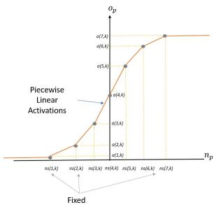
Figure 8: Piecewise Linear Curve

figure 8, show a PWL activation for K hidden units which consists of multiple ramps where, $ns(1,k)$ is the first hinge of the $k^{th}$ hidden unit and $a(1,k)$ is its activation value. These hinge values $ns$ are constant throughout training. From the figure we can observe that the PWL curve which passes through the activation of each of the 7 hinges. We define total number of hinges as $H$. The equation for above figure is given in equation 45. Let $s$ denote maximum value of a net function and $r$ denote minimum value of net function. The activations are calculated between two points, where, the net values between first two hinges are calculated with $ns(1,k)$ denoted as $m_{1}$ and $ns(2,k)$ denoted as $m_{2}$. Similarly, activations output between next two hinges are calculated by denoting $ns(2,k)$ denoted as $m_{1}$ and $ns(3,k)$ denoted as $m_{2}$. We do this for $H$ hinges. $m_{1}$ and $m_{2}$ for each hinge is calculated as $m_{1}=\lceil\frac{n_{p}}{\delta ns}\rceil$ and $m_{2}=m_{1}+1$. Given the net function $n_{p}(k)$, $o_{p}(k)$ is calculated as,

$$w_{1p}(k)=\frac{ns(m_{2},k)-n_{p}(k)}{ns(m_{2},k)-ns(m_{1},k)}$$ (43)

$$w_{2p}(k)=\frac{n_{p}(k)-ns(m_{1},k)}{ns(m_{2},k)-ns(m_{1},k)}$$ (44)

$$o_{p}(k)=\Bigg{\{}\begin{matrix}a(H,k)\\ w_{1p}(k)\cdot a(m_{1},k)+w_{2p}(k)\cdot a(m_{2},k)\\ a(1,k)\end{matrix}\hskip 28.45274pt\begin{matrix}for\quad n_{p}(k)>s\\ for\quad s>n_{p}(k)>r\\ for\quad n_{p}(k)<r\end{matrix}\Bigg{\}}$$ (45)

where, $w_{1p}(k)$ and $w_{2p}(k)$ are the slope equation for each of the two hinges for $k^{th}$ hidden unit. ${n}_{p}(k)$ is the $p^{th}$ pattern and $k^{th}$ hidden unit net function and $o_{p}(k)$ is its activation function. For all the activation values less $ns(1,k)$ has zero slope hence $n_{p}(k)$ = $a(1,k)$. Similarly, for all the values greater than $ns(H,k)$ has zero slope therefore, $n_{p}(k)$ = $a(H,k)$.

4.3 Example of PWL activation calculation

For initialization of PWL activation, we first need to initialize the PWL using the most widely used activations such as sigmoid[36], relu[31] and leaky relu[32], etc. We then decide total number $H$ on the net function. This method can be done individually for each of the hidden units. In this dissertation, we use same number of $ns$ hinges for each of the hidden units. We then find the minimum and maximum hinge values from the net function output. This is achieved by randomly selecting data from each of the classes and performing convolution and then selecting the minimum and maximum value from the output of the convolution.

Below, we show the calculation for PWL activations for $k=1$ hidden unit as follows. As discussed above we first need to find the initial activation. For this example we use sigmoid activation as shown in figure 9

Figure 9: Sigmoid Curve

From the figure we can see that $x$ axis is the net function $n_{p}$ and the $y$ axis is its corresponding sigmoid activation. The range of sigmoid is from $0$ to $1$. Step 2 is finding the minimum and maximum value from convolution output. In this case, we select the values as $-4$ and $4$. Now, we need to decide $ns$ samples on the sigmoid curve. This step is user choosen. Here, for this example we choose $H=7$. We show our selection of hinges and activations in table format as show in Table 1

H	1	2	3	4	5	6	7
Fixed hinges ($ns_{1}$)	-4	-2.67	-1.33	0	1.33	2.67	4
Activations for hinges($a_{1}$)	0.02	0.07	0.21	0.5	0.79	0.94	0.98

Table 1: PWL samples and activations for one hidden unit

From table 1, we can see that there are total $H=7$ hinges ranging from -4 to 4, which are our minimum and maximum values from the net function and its sigmoid activations as activation samples $a$. Finally we plot these points on the sigmoid curve from figure 9. The curve after plotting these points should look like figure 10

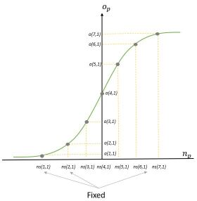
Figure 10: Sigmoid with Fixed Samples

figure 10 is the plot for a fixed piecewise sigmoid activation for net versus activations values where $7$ hinges are plotted on to the sigmoid curve. Now, for the final piecewise linear curve we remove the sigmoid curve and linearly join 2 points using linear interpolation technique.

Linear interpolation involves estimating a new value of a function between two known fixed points [75][76].

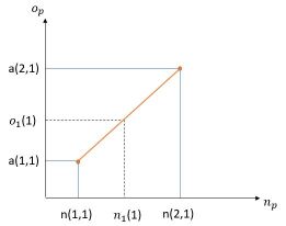
Figure 11: Linear interpolation between 2 points

figure 11 relates the use of linear interpolation between 2 fixed $ns$ points. We can say that if we have a new sample net value $n_{1}(1)$, its corresponding activation value is as shown in the figure. To find $o_{1}(1)$ between $a(1,1)$ and $a(2,1)$, we use the following equation.

$$o_{1}(1)=\frac{ns(2,1)-n_{1}(1,1)}{ns(2,1)-ns(1,1)}\cdot a(1,1)+\frac{n_{1}(1)-ns(1,1)}{ns(2,1)-ns(1,1)}\cdot a(2,1)$$ (46)

Finally, we use the equation 45 to find all the activation output, The plot of net versus activation is shown in figure 8.

4.4 PLA gradients

Above discussed PWL activations A are trained via steepest descent. The negative gradient matrix $\mathbf{G_{a}}$ with respect to $E_{ce}$ is calculated as,

$${g_{a}(k,m)}=-\frac{\partial E_{ce}}{\partial{a(k,m)}}$$ (47)

where $k$ is the hidden unit number and $m$ is the $H^{th}$ hinge.

$${g_{a}(k,m)}=\frac{2}{N_{v}}\sum_{p=1}^{N_{v}}\sum_{i=1}^{M}(t_{p}(i)-y_{p}(i))\cdot\frac{\partial y_{p}(i)}{\partial{a(u,m)}}$$ (48)

$$\frac{\partial y_{p}(i)}{\partial{a(u,m)}}=w_{oh}(i,u)\cdot\frac{\partial o_{p}(i)}{\partial{a(u,m)}}$$ (49)

$$\frac{\partial o_{p}(i)}{\partial{a(u,m)}}=w_{oh}(i,u)\cdot((\delta(m-m_{1})\cdot w_{1}(p,u))+(\delta(m-m_{2})\cdot w_{2}(p,u)))$$ (50)

where, for the $p^{th}$ pattern and $k^{th}$ hidden unit of the net value we find $m_{1}$ and $m_{2}$, where the $p^{th}$ pattern of $k^{th}$ hidden unit of the net value lies between the two fixed piecewise linear sample values $m_{1}$ and $m_{2}$ of the $u^{th}$ hidden unit as described in the search algorithm. Also we need to find $w_{1}(p,u)$ and $w_{2}(p,u)$ from equations 43 and 44. A search algorithm is used to find the correct $m$ sample for a particular pattern’s hidden unit is found[72]. The equation 50 solves for the $p^{th}$ patterns $u^{th}$ hidden unit of the piecewise linear activations and accumulates the gradient for all the $p^{th}$ patterns of their respective $u^{th}$ hidden units.

Adams optimizer[57] is used to find learning factor and update the weights of the activation. which are updated as follows

$$\mathbf{A}=\mathbf{A}+z\cdot\mathbf{G_{a}}$$ (51)

4.5 PLA OLF

Using the gradient $\mathbf{G_{a}}$, the optimal learning factor for activations training is calculated as, The activation function vector $\textbf{o}_{p}$ can be related to its gradient as,

$$\mathbf{o}_{p}(k)=w_{1}(p,k)\cdot[a(k,m_{1})+z\cdot g_{o}(k,m_{1})]+w_{2}(p,k)\cdot[a(k,m_{2})+z\cdot g_{o}(k,m_{2})]$$ (52)

The first partial derivative of E with respect to z is

$$\frac{\partial E}{\partial z}=\frac{2}{N_{v}}\sum_{p=1}^{N_{v}}\sum_{i=1}^{M}(t_{p}(i)-y_{p}(i))\cdot\frac{\partial y_{p}(i)}{\partial{z}}$$ (53)

where

$$\frac{\partial y_{p}(i)}{\partial{z}}=\sum_{k=1}^{N_{h}}w_{oh}(i,k)\cdot((w_{1}(p,k)\cdot g_{o}(k,m_{1}))+(w_{2}(p,k)\cdot g_{o}(k,m_{2})))$$ (54)

where, $m_{1}$ and $m_{2}$ for the $p^{th}$ pattern and $k^{th}$ hidden unit of the net vector $n_{p}(k)$ is again found, and find $g_{o}(k,m_{1})$ and $g_{o}(k,m_{2})$ from the gradient calculated from equations (48, 49, 50)

Also the Gauss-Newton[77] approximation of the second partial is

$$\frac{\partial^{2}E(z)}{\partial z^{2}}=\frac{2}{N_{v}}\sum_{p=1}^{N_{v}}\sum_{i=1}^{M}\left[\frac{\partial y_{p}(i)}{\partial{z}}\right]^{2}$$ (55)

Thus the learning factor is calculated as

$$z=\frac{\frac{-\partial^{2}E(z)}{\partial z^{2}}}{\frac{\partial E}{\partial z}}$$ (56)

After finding the optimal learning factor the piecewise linear activations, $\mathbf{A}$, are updated in a given iteration as

$$\mathbf{A}=\mathbf{A}+z\cdot\mathbf{G_{a}}$$ (57)

where $\mathbf{z}$ is a scalar optimal learning factor and $\mathbf{G_{a}}$ is the gradient matrix calculated in equation 56 and 47.

The ADAPT-ACT-OLF algorithm can be summarized as follows:

Algorithm 4 ADAPT-ACT-OLF algorithm

1:Initialize $\mathbf{W,W_{oi},W_{oh}}$, $N_{it}$

2:Initialize Fixed hinges $\mathbf{ns}$ and hinge activation $\mathbf{a}$ as described in sub section 4.3 , it$\leftarrow$ 0

3:while it $<$ $N_{it}$ do

4:     Find gradient $G$ and $G_{hwo}$ from equations 47 and 22.

5:     Find learning factor $z$

6:     Calculate gradient and learning factor for activation from equation 47 and equation 56 respectively and update the activations as in equation 57.

7:     OWO step : Solve equation (19) to obtain $\mathbf{W_{o}}$

8:     it $\leftarrow$ it + 1

9:end while

4.6 PLA adavantages(sine example with a theory on why it should be used with initialization of relu, leaky relu)

In this subsection, we demonstrate the advantage of adaptive activations using a simple sine data function and a more complicated rosenbrock function. We will be training the Basic MOLF-ADAPT algorithm explained in section. For each of the experiment, we will be using a constant activation from sigmoid,tanh,relu and leaky relu and will compare with ADAPT-ACT-OLF algorithm with initial activations as sigmoid, tanh, relu and leaky relu respectively.

4.6.1 Sinusoidal Approximation

The sine data is generated using one feature and 5000 uniformly distributed random samples in the range of $0$ to $4pi$. The output generated is the sine function of the uniformly distributed random samples.

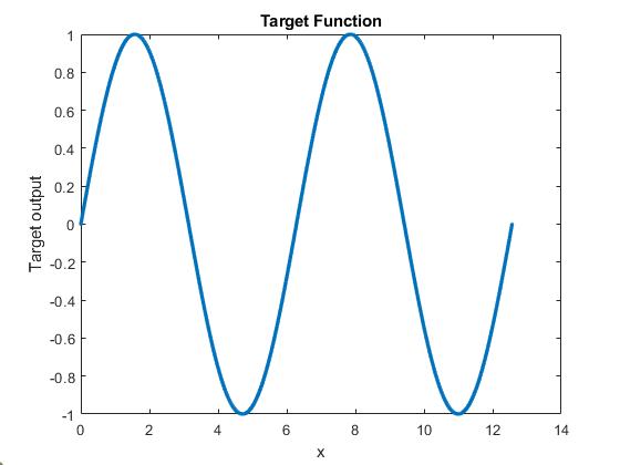
Figure 12: Sine Training Data

Fig 12 shows Input versus Target output plot where $x$ is the input which is in the range of $0$ to $4pi$ and the Target ouput is the sine of inputs. Looking at the plot one can assume that a sigmoid or a tanh activation would work better than relu or leaky relu.

In the following section, we will train a Basic MOLF-ADAPT algorithm with each of the above mentioned activations. Similarly, we will use ADAPT-ACT-OLF algorithm with respective initial activations. The number of hidden units we will be using is one and 10 respectively. From our understanding we believe that sigmoid and tanh activations will work better for the sinusoidal data with relu and leaky relu failing as compared to sigmoid and tanh. So we will start with relu and leaky relu followed by sigmoid and tanh activation results.

ReLU Activation

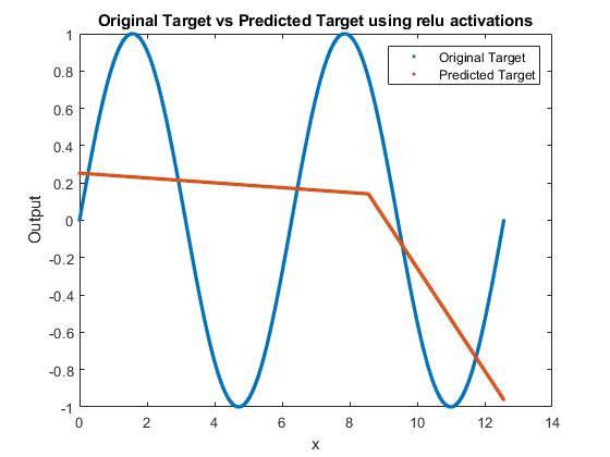
(a) ReLU Activations with 1 Nh

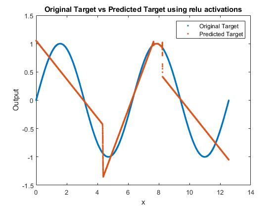
(b) ReLU Activations with 10 Nh

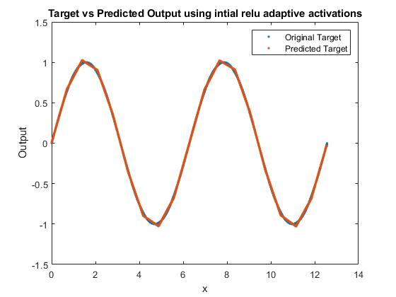
(c) ReLU Adaptive Activations with 20 samples

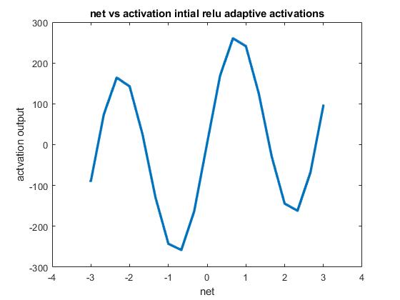
(d) Adaptive hidden unit using intial ReLU activation

Figure 13: Relu activations output

Figure 13 shows the Basic MOLF-ADAPT and ADAPT-ACT-OLF results using ReLU as the activation function where 13(a) is the input versus ouput using one fixed ReLU activation. We can observe that using one hidden unit ReLU activation cannot approximate the simple sinusoidal function. Now, we increase our hidden unit size to 10 and we can still observe from figure 13(b) that relu activation still cannot approximate the sinusoidal curve, This can be due to the fixed relu acitivation. Now we use relu as an initial activation function for adaptive activation and based on multiple experimentations we observed that to achieve better results for sinusoidal, more samples should be used. In this particular experimentation we used 20 samples. From figure 13(c) we we see that using adaptive activation the model was able to approximate better than fixed relu activations. From the figure we can also observe that adaptive activations fails to approximate the curve accurately. This problem can be elimiated by adding more samples. From our experimentation, we observed that by using 40 samples the approximation is similar to the fixed sigmoid activations, but this comes with the increase computational cost. But we can conclude that adaptive activation with relu as intital activation works better than the fixed activation. Next we will look at leaky relu activation with alpha value as 0.01. As it is similar to relu except for in negative net values, we should expect similar results. Also, figure 13(d) shows the single hidden unit after training and we can observe that the net vs activation output mimics the output curve but with high activations output

Leaky ReLU Activation

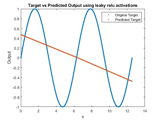
(a) Leaky ReLU Activations with 1 Nh

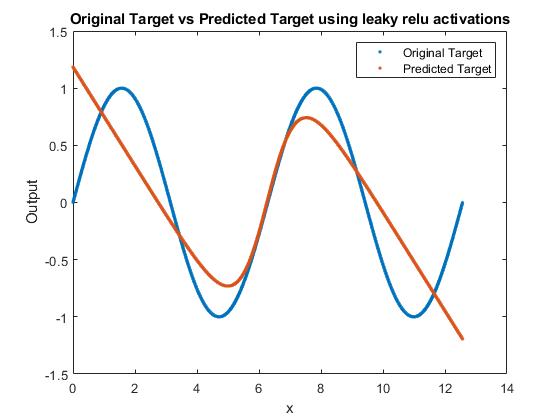
(b) Leaky ReLU Activations with 10 Nh

(c) Leaky ReLU Adaptive Activations with 20 samples

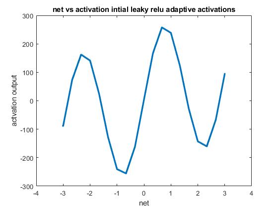
(d) Adaptive hidden unit using intial Leaky ReLU activation

Figure 14: Leaky Relu activations output

Figure 14 shows the Basic MOLF-ADAPT and ADAPT-ACT-OLF results using Leaky ReLU as the activation function where 13(a) is the input versus ouput using one fixed Leaky ReLU activation. We can observe from figure 14(a) and 14(b) leaky relu does not approximate the sinusoidal as similar to relu activation. But from figure 14(c) we can observe that adaptive activations work better again and almost similar to relu activations. Even the net vs activation output from figure 14(d) is similar to the relu activations.

Sigmoid Activation

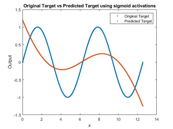
(a) Sigmoid Activations with 1 Nh

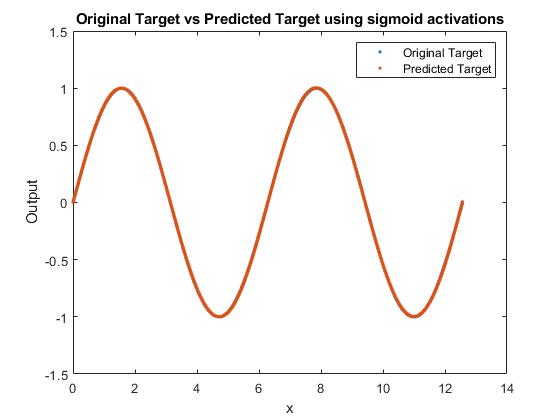
(b) Sigmoid Activations with 10 Nh

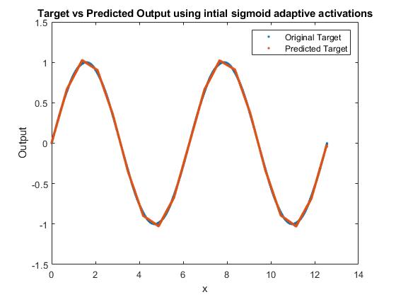
(c) Adaptive Activations with 20 samples

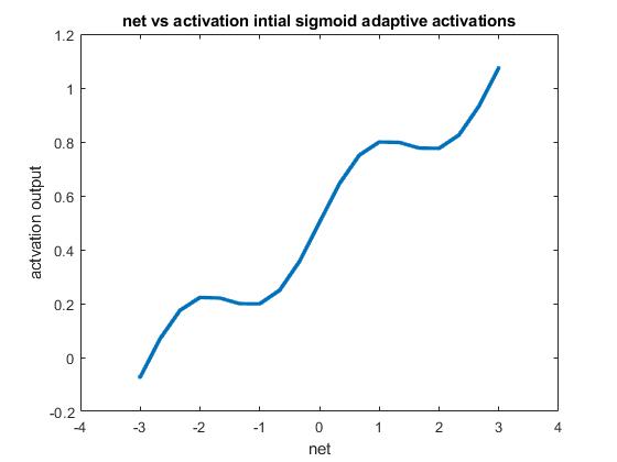
(d) Adaptive hidden unit using intial sigmoid activation

Figure 15: Sigmoid activations output

Figure 15 shows the Basic MOLF-ADAPT and ADAPT-ACT-OLF results where 15(a) is the input versus ouput using one fixed sigmoidal activation. We can observe that using one hidden unit is not sufficient to approximate the simple sinusoidal function. Now as we increase our hidden unit to 10 the training approximates a sinusoidal curve as it is evident from figure 15(b). Now we will discuss the results with adaptive activations where the initial hidden unit is sigmoid. For the number of samples we chose 20 samples as we observed that if the input output is a curve function, more number of samples are needed as our adaptive activation is piecewise linear. From figure 15(c) we can observe that the linear part of the sinusoidal curve is approximated well but because of the linearity of the adaptive activations it fails to approximate the curve accurately. This problem can be elimiated by adding more samples. From our experimentation, we observed that by using 40 samples the approximation is similar to the fixed sigmoid activations, but this comes with the increase computational cost. Figure 15(d) which shows the net vs activation graph which does not mimic exact similar graph to sigmoid but is close to sigmoid with smaller peaks at each of the positive and negative activation axis. Also thing to note is that the activation output values are very small as compared to the relu and leaky relu activations shown in paragraph 4.6.1 and 4.6.1

TanH Activation

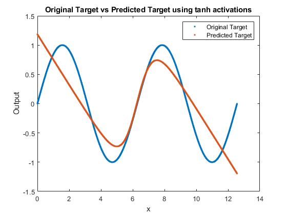
(a) Tanh Activations with 1 Nh

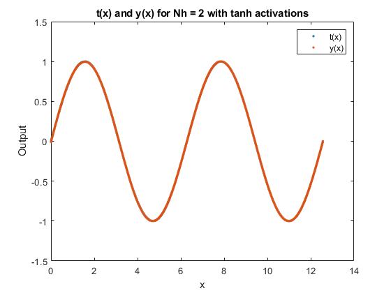
(b) Tanh Activations with 10 Nh

(c) Tanh Adaptive Activations with 20 samples

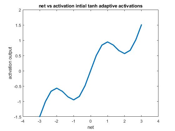
(d) Adaptive hidden unit using intial Tanh activation

Figure 16: Tanh activations output

Figure 16 shows the Basic MOLF-ADAPT and ADAPT-ACT-OLF results where 16(a) is the input versus ouput using one fixed Tanh activation. We can observe that using one hidden unit is not sufficient to approximate the simple sinusoidal function. Now as we increase our hidden unit to 10 the training approximates a sinusoidal curve as it is evident from figure 16(b). Now we will discuss the results with adaptive activations where the initial hidden unit is sigmoid. For the number of samples we chose 20 samples as we observed that if the input output is a curve function, more number of samples are needed as our adaptive activation is piecewise linear. From figure 16(c) we can observe that the linear part of the sinusoidal curve is approximated well but because of the linearity of the adaptive activations it fails to approximate the curve accurately. This problem can be elimiated by adding more samples. From our experimentation, we observed that by using 40 samples the approximation is similar to the fixed sigmoid activations, but this comes with the increase computational cost.Figure 16(d) which shows the net vs activation graph which does not mimic exact similar graph to sigmoid but is more closer to the sinusoidal curve than sigmoidal adaptive activation. Also thing to note is that the activation output values are very small as compared to the relu and leaky relu activations shown in paragraph 4.6.1 and 4.6.1

To conclude, Using fixed activation to approximates a sinusoidal curve does not yeild promising results for every activation especially the ones without curve in the function which according to our experimentation is relu and leaky relus. But using adaptive activation, the model converges to the same output with any initial activation with the hidden unit trying to mimic the output curve. After multiple experimentation we can conclude that to achieve sinusoidal curve, more samples are needed to achieve the smooth curve

4.6.2 Rosenbrock Approximation

In this subsection we demonstrate approximation of the rosenbrock[78]. The input is generated using constant values a= 1 and b = 100 and total of 1000 uniformly distributed random samples are generated for each of the two inputs. The output generated is the rosenbrock[78] function. Here we normalize both the inputs and outputs with zero mean and standard deviation on 1 for ease of training. We saw no difference in results

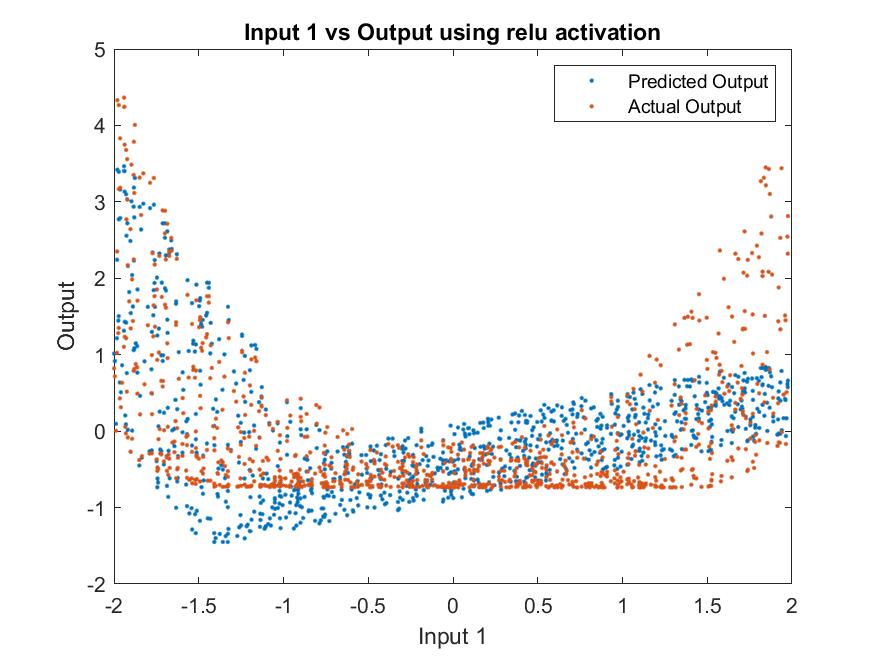
(a) ReLU Activations Input 1 vs Output

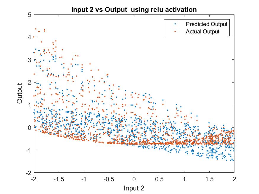
(b) ReLU Activations Input 2 vs Output

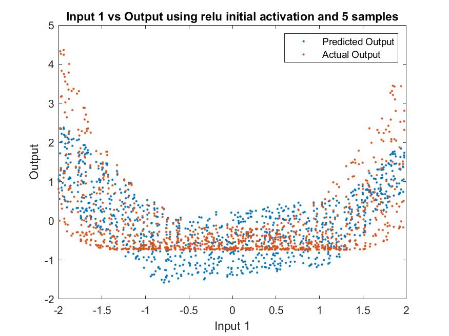
(c) Adaptive ReLU Activations Input 1 vs Output for 5 samples

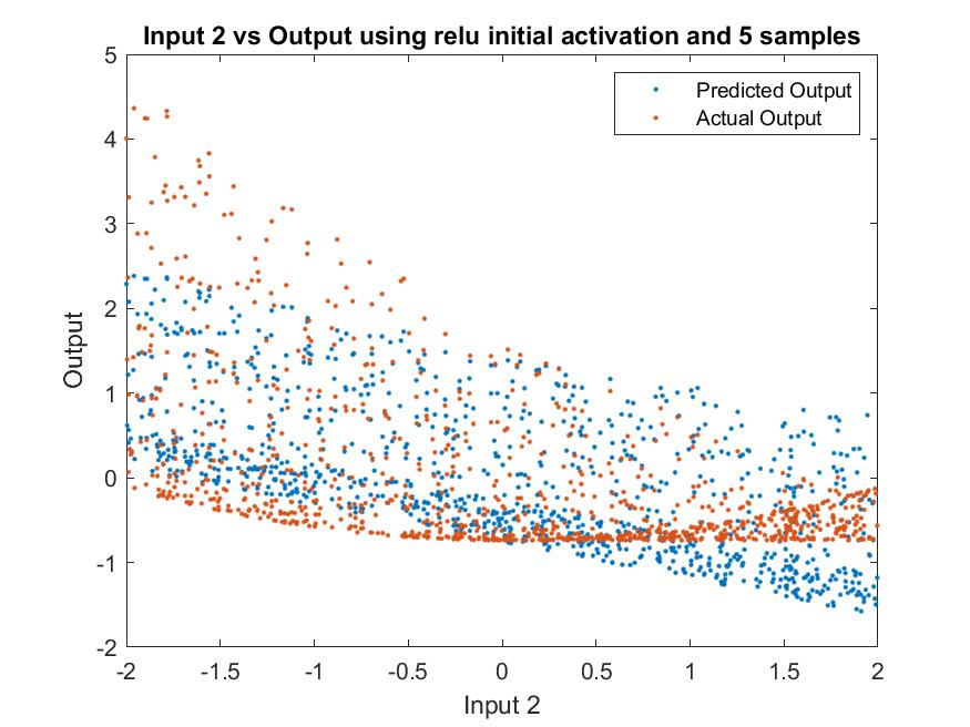
(d) Adaptive ReLU Activations Input 2 vs Output for 5 samples

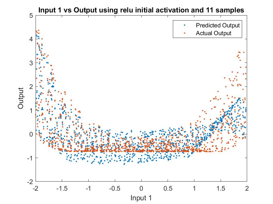
(e) Adaptive ReLU Activations Input 1 vs Output for 11 samples

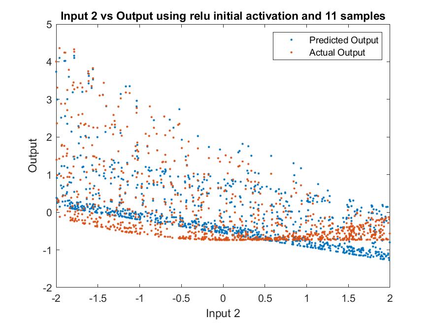
(f) Adaptive ReLU Activations Input 2 vs Output for 11 samples

Figure 17: Rosenbrock Approximation with ReLU Activations

Figure 17(a) shows input 1 versus Output for a MLP trained using ReLU activations. In 17(a), we can see a scatter plot of predicted versus the actual output. We can observe that it does not approximate accurately. But when we observe figure 17(c) and figure 17(f) which are the results for adaptive activations training with 5 samples and 11 samples respectively. The approximation there is not as accurate as the actual output but is better than the model trained using relu activation. Similarly, Figure 17(b) shows input 2 versus Output for a MLP trained using ReLU activations. Again, we can see that the approximation is not as accurate. But when we observe figure 17(d) and figure 17(d) which are the results for adaptive activations training with 5 samples and 11 samples respectively. The approximation there is not as accurate as the actual output but is better than the model trained using relu activation

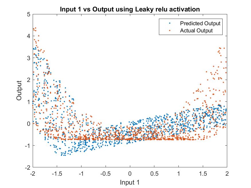
(a) Leaky ReLU Activations Input 1 vs Output

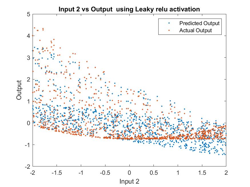
(b) Leaky ReLU Activations Input 2 vs Output

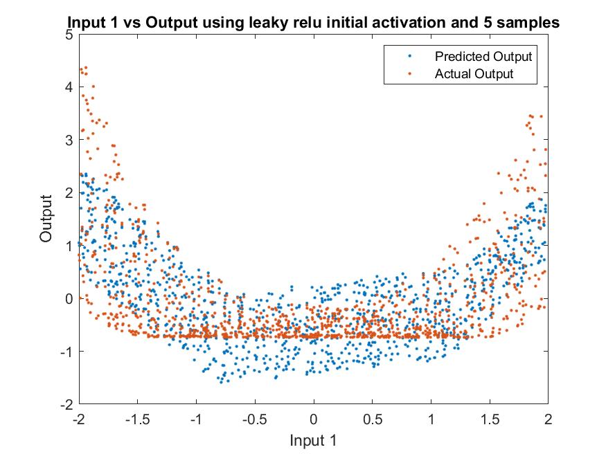
(c) Leaky Adaptive ReLU Activations Input 1 vs Output for 5 samples

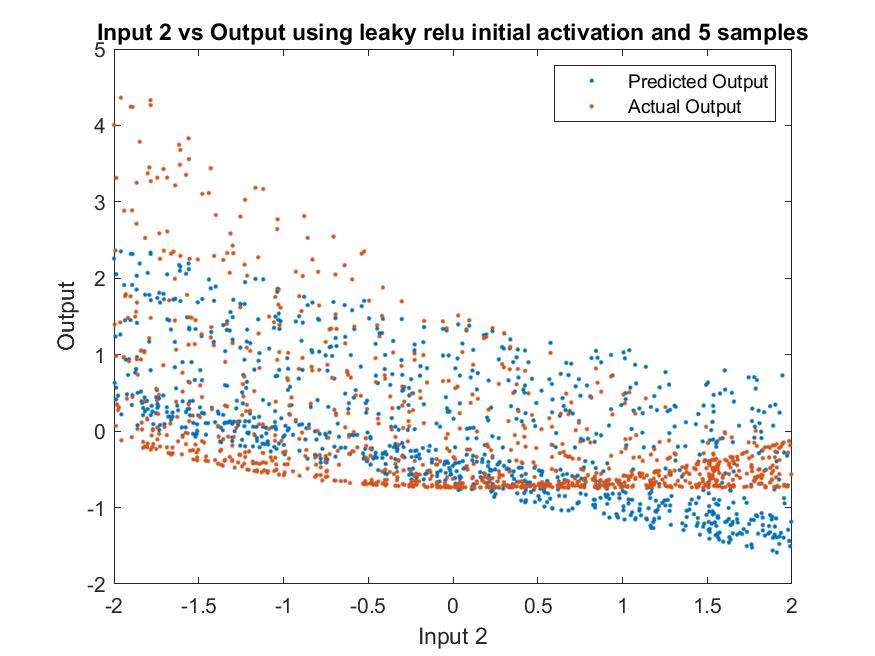
(d) Leaky Adaptive ReLU Activations Input 2 vs Output for 5 samples

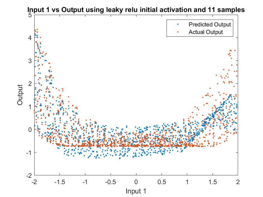
(e) Leaky Adaptive ReLU Activations Input 1 vs Output for 11 samples

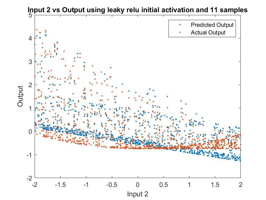
(f) Leaky Adaptive ReLU Activations Input 2 vs Output for 11 samples

Figure 18: Rosenbrock Approximation with Leaky ReLU Activations

Figure 18(a) shows input 1 versus Output for a MLP trained using Leaky ReLU activations. In 18(a), we can see a scatter plot of predicted versus the actual output. We can observe that it does not approximate accurately. But when we observe figure 18(c) and figure 18(f) which are the results for adaptive activations training with 5 samples and 11 samples respectively. The approximation there is not as accurate as the actual output but is better than the model trained using relu activation. Similarly, Figure 18(b) shows input 2 versus Output for a MLP trained using Leaky ReLU activations. Again, we can see that the approximation is not as accurate. But when we observe figure 18(d) and figure 18(d) which are the results for adaptive activations training with 5 samples and 11 samples respectively. The approximation there is not as accurate as the actual output but is better than the model trained using Leaky relu activation

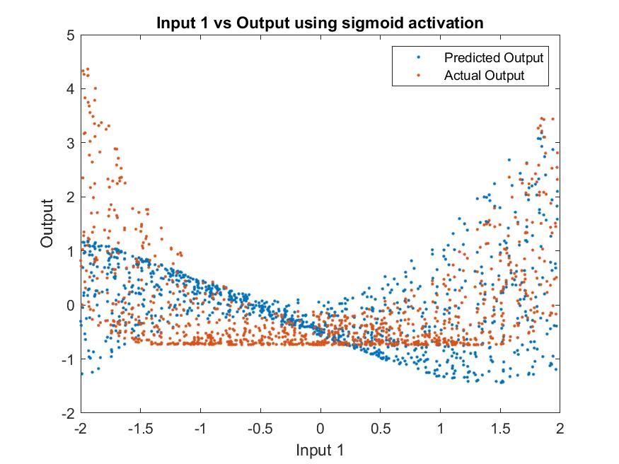
(a) Sigmoid Activations Input 1 vs Output

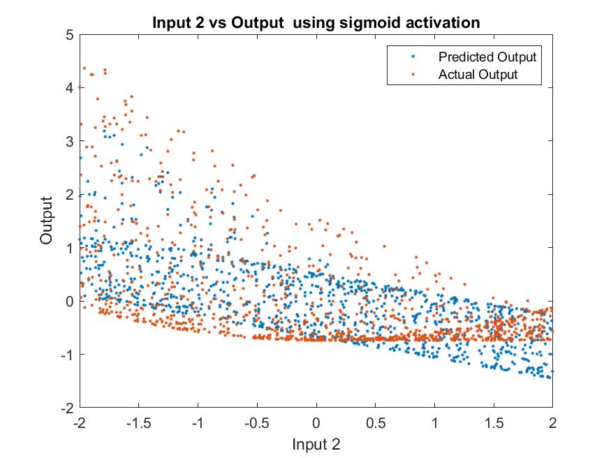
(b) Sigmoid Activations Input 2 vs Output

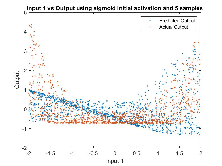
(c) Adaptive Sigmoid Activations Input 1 vs Output for 5 samples

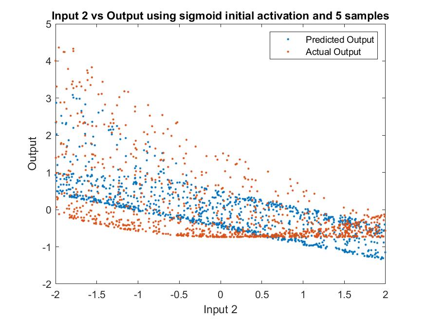
(d) Adaptive Sigmoid Activations Input 2 vs Output for 5 samples

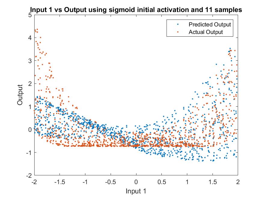
(e) Adaptive Sigmoid Activations Input 1 vs Output for 11 samples

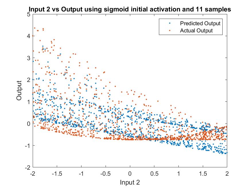
(f) Adaptive Sigmoid Activations Input 2 vs Output for 11 samples

Figure 19: Rosenbrock Approximation with Sigmoid Activations

Figure 19(a) shows input 1 versus Output for a MLP trained using Sigmoid activations. In 19(b), we can see a scatter plot of predicted versus the actual output. We can observe that it does not approximate accurately. But when we observe figure 19(c) and figure 19(d) which are the results for adaptive activations training with 5 samples and 11 samples respectively. The approximation rsults with 5 samples are not as good but results with 11 samples are better than the model trained using Sigmoid activation. Similarly, Figure 19(b) shows input 2 versus Output for a MLP trained using Sigmoid activations. Again, we can see that the approximation is not as accurate. But when we observe figure 19(e) and figure 19(f) which are the results for adaptive activations training with 5 samples and 11 samples respectively. The approximation there is not as accurate as the actual output but is better than the model trained using Sigmoid activation

(a) TahH Activations Input 1 vs Output

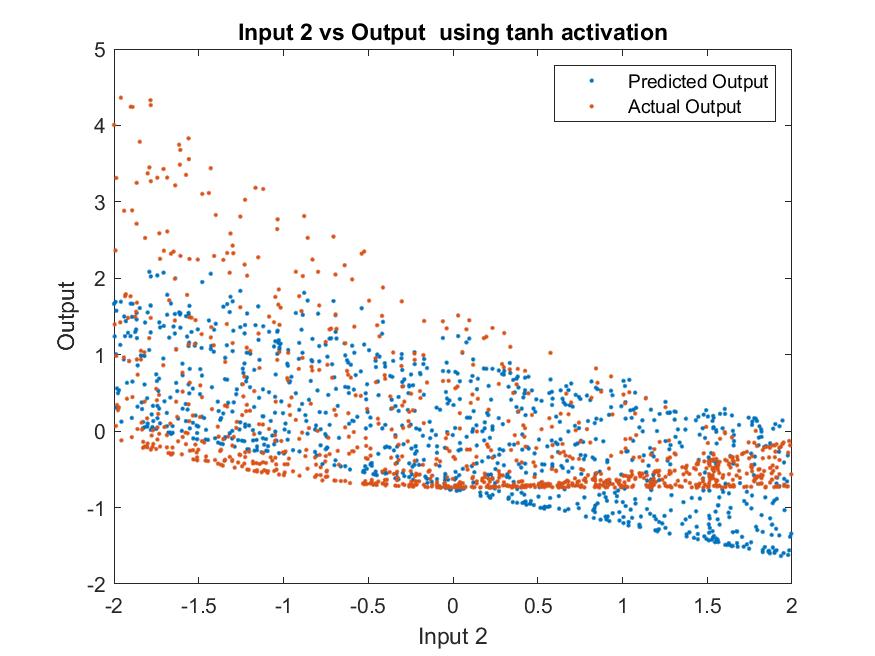
(b) TanH Activations Input 2 vs Output

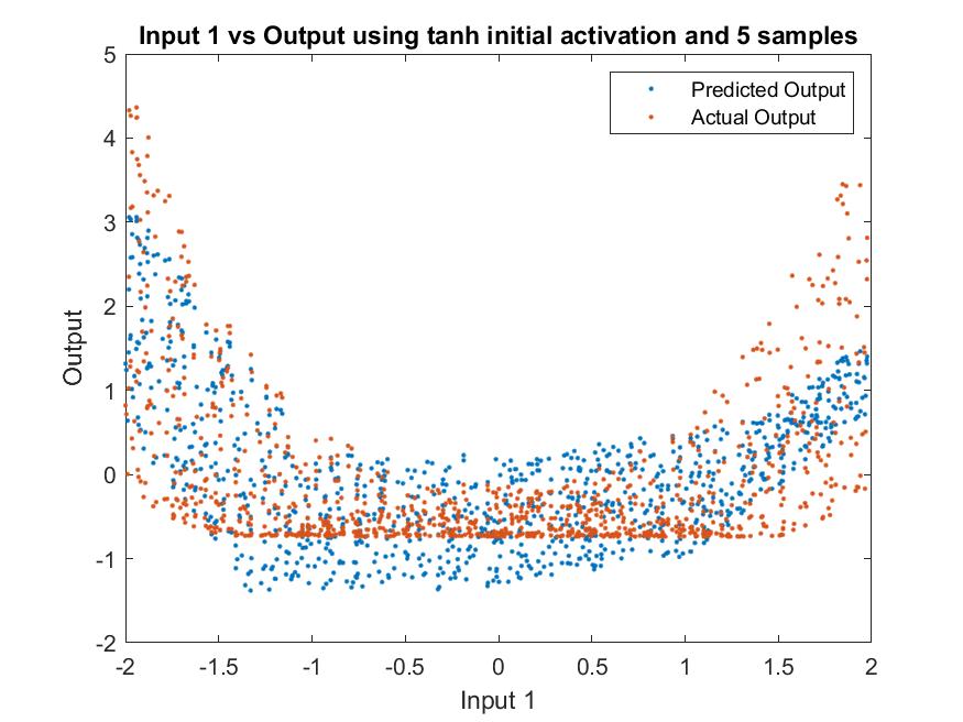
(c) Adaptive Tanh Activations Input 1 vs Output for 5 samples

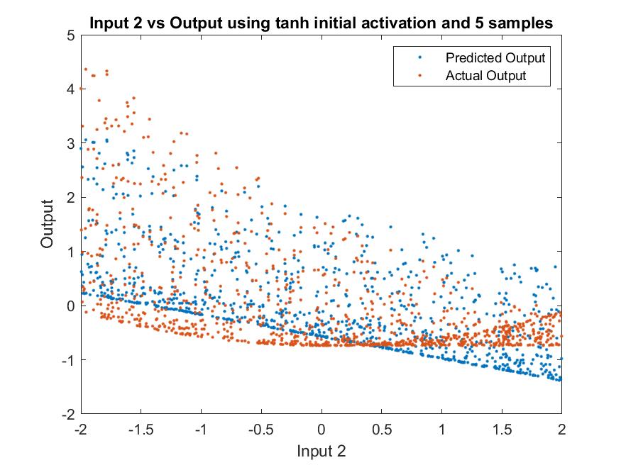
(d) Adaptive Tanh Activations Input 2 vs Output

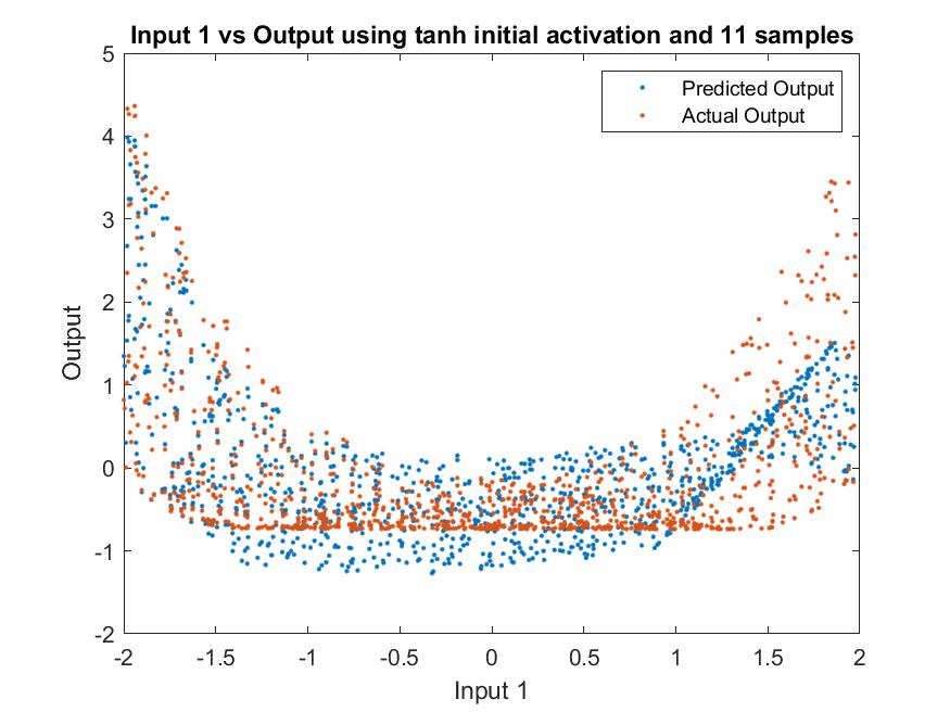
(e) Adaptive Tanh Activations Input 1 vs Output

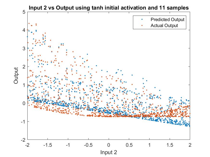
(f) Adaptive Tanh Activations Input 2 vs Output

Figure 20: Rosenbrock Approximation with Tanh Activations

Figure 20(a) shows input 1 versus Output for a MLP trained using TahH activations. In 20(b), we can see a scatter plot of predicted versus the actual output. We can observe that it does not approximate accurately. But when we observe figure 20(c) and figure 20(d) which are the results for adaptive activations training with 5 samples and 11 samples respectively. The approximation rsults with 5 samples are not as good but results with 11 samples are better than the model trained using TahH activation. Similarly, Figure 20(b) shows input 2 versus Output for a MLP trained using TahH activations. Again, we can see that the approximation is not as accurate. But when we observe figure 20(e) and figure 20(f) which are the results for adaptive activations training with 5 samples and 11 samples respectively. The approximation there is not as accurate as the actual output but is better than the model trained using TahH activation

5 Experimental Methods and Results

In this section, we discuss experiment results for the proposed algorithm in which we demonstrate relative testing results for widely available approximation and classification data. Finally, we show results for a shallow convolutional neural network architecture.The computational cost is measured on a Windows 10, Intel i-7, 3 Mhz CPU platform with 32 GB RAM.

In this section, we demonstrate network performance comparison between ADAPT-ACT-OLF, ADAPT-ACT-OLF,CG-MLP[79] [66][61] and LM [80][81] for approximation and classification data. We also show results for shallow convolution neural networks with custom networks and deep CNNs using transfer learning.

5.1 Approximation Datasets Results

Dataset	SCG/Nh	CG-MLP/Nh	LM/Nh	MOLF-ADAPT $L_{R}elu/Nh$	Adapt-OLF 3samples/Nh	Adapt-OLF 5 samples/Nh	Adapt-OLF 9samples/Nh
Oh7	1.971/30	1.52/100	${\mathbf{1.41}/30}$	1.51/15	1.49/20	1.46/20	1.44/15
White Wine	0.6/20	0.56/100	0.57/30	0.55/30	${\mathbf{0.54/100}}$	0.56/20	${\mathbf{0.54/100}}$
twod	0.5/30	0.23/100	0.17/15	${\mathbf{0.149/15}}$	${\mathbf{0.149/15}}$	0.18/15	0.15/15
Superconductor	230.91/15	180.21/100	170.2/100	144.46/100	142.53/100	${\mathbf{139.62/100}}$	142.53/100
F24	1.14/20	0.31/100	0.30/30	0.281/100	0.282/100	0.283/100	${\mathbf{0.279/100}}$
Concrete	61.11/5	34.64/30	32.12/20	32.29/100	${\mathbf{30.70/100}}$	34.34/10	35.56/100
Weather	316.68/15	283.23/30	286.27/30	${\mathbf{283.20/10}}$	284.39/15	284.34/15	284.73/15

Table 2: 10-fold cross validation mean square error (MSE) testing results for approximation dataset, (best testing MSE is in bold)

From the Table 2, we can observe that Adapt-OLF is the top performer in 5 out of the 7 data sets in terms of testing MSE. The following best-performing algorithm is MOLF-ADAPT for weather data which is with smaller margin and is also tied in comparison to testing MSE for twod dataset. Adapt-OLF has slightly more number of parameters depending on the number of samples but the testing MSE is substantial reduced. Next best performer is LM for the oh7 dataset. However, LM being a second-order method, its performance comes at a significant cost of computation – almost two orders of magnitude greater than the rest. of the models proposed

5.2 Classifier Datasets Results

Dataset	SCG/Nh	CG-MLP/Nh	LM/Nh	MOLF-ADAPT $L_{R}elu/Nh$	Adapt-OLF 3samples/Nh	Adapt-OLF 5 samples/Nh	Adapt-OLF 9samples/Nh
GongTrn	10.28/100	10.46/100	8.94/30	${\mathbf{8.62}}$/30	8.65/30	8.64/30	8.72/30
Comf18	15.69/100	14.50/100	12.63/5	11.83/20	11.93/30	11.87/30	${\mathbf{11.79/30}}$
f17c	3.22/100	3.69/100	3.96/100	2.45/100	2.38/100	2.41/100	${\mathbf{2.34/100}}$
Speechless	44.26/100	43.07/100	39.72/100	36.65/100	${\mathbf{35.96/100}}$	38.94/100	37.6/100
Cover	27.39/100	29.87/100	NA	20.1/30	19.43/30	19.47/30	${\mathbf{19.42/30}}$
Scrap	25.58/100	20.77/100	NA	19.9/100	19.57/100	${\mathbf{18.8/100}}$	19.2/100

Table 3: 10-fold cross validation Percentage of Error (PE) testing results for classification dataset, (best testing MSE is in bold)

From the Table 3, we can observe that Adapt-OLF is the top performer in 5 out of the 6 data sets in terms of testing MSE. The following best-performing algorithm is MOLF-ADAPT for weather data which is with smaller margin. As LM requires significant cost of computation it cannot be used for pixel based inputs hence loses out on majority of the image classification based use cases

5.3 CNN Results

5.3.1 Shallow CNN results

In this section, we demonstrate shallow CNN results with relu, leaky relu and adaptive activations. We will be using a one VGG block [82], two vggg block and three VGG block. We will also be using cifar 10 dataset for benchmarking our results. Figure 21 is the One VGG block.

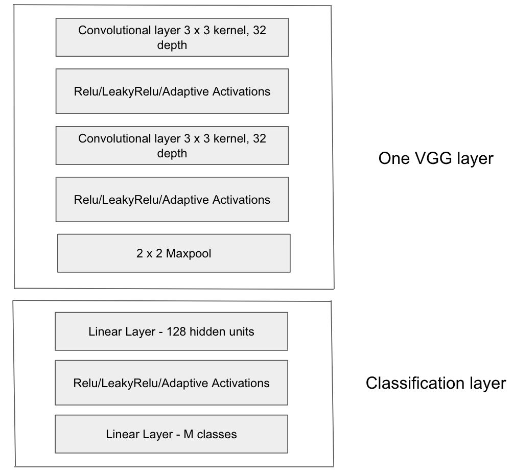
Figure 21: One VGG layer with classifier

From Figure 21 we can see that there is one VGG layer and a classification layer. The one VGG layer consists of 2 convolution layers with 3x3 kernel and 32 filters in the first and and 3rd layer and activations are in 2nd and 4th layer. The final layer is a 2 x 2 maxpool layer. Similarly two VGG layer has 2 vgg layers and one classification layer where the first vgg layer has the same configuration as in the figure with 32 filters and the 2nd vgg layer consists of convolution layers with 3 x 3 kernels and depth as 64 for each convolution layer as shown in Figure 22

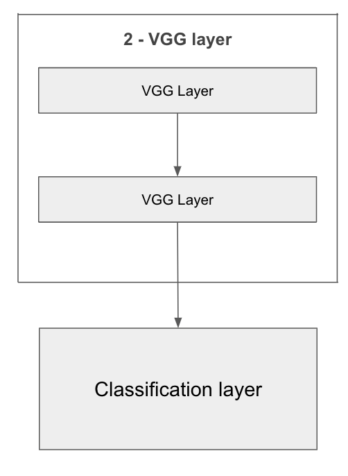
Figure 22: Two VGG layer with classifier

Similarly, in 3 VGG layer, we have 2 vgg layers as mentioned above and a 3rd vgg layer has the same configuration as the 2nd vgg layer with 3 x 3 kernels but the depth is 64 filters for each convolution layer as shown in Figure 23

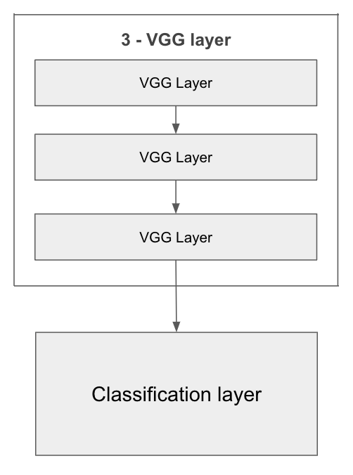
Figure 23: Three VGG layer with classifier

One thing to note here is that when the model is used with relu activations are used all the activations used are relu, similarly with leaky relu but in adaptive activations the last VGG layer activations are trained and the remaining are not trained and are either kept as relu or leaky relu. For example, In 2 - VGG layer, the 2nd VGG layer’s adaptive activation functions are trained and the first VGG layers adaptive activations are not used as trainable parameters. The number of samples(n) used in the activations for the below experiment are kept as 3 as follows [minimum value, 0, maximum value], where the first is the minimum value of the output of the convolution layer before the adaptive activation, the second value is 0 and the final value is maximum value of the output of the convolution layer before the adaptive activation layer. For example, if we are training a 2 VGG layer model, as described above, activations in the VGG1 layer are not trained. The out put of the VGG1 layer that is the 2 x 2 maxpool output is used a input to the 2nd VGG layer where th output of the first convolution layer’s maximum and minimum value in the 2nd VGG layer is used. The activation function used in the adaptivations where the activations are not trainable are leaky relu and also the initialization of the adaptive activaions are done using leaky relu. As suggested earlier, any activations can be used in the intialization. The decision here was taken based on the results seen in the Table 4 for the model with leaky relu activations.

Table 4 shows results for 1-vgg layers, 2-vgg layers, 3-vgg layers model on CIFAR10[46] dataset with Glorot normal initialization From the table we can observe that as the number of vgg layer increase, adaptive activation gives better accuracy. One thing to note is that in 3-VGG layer model only the 3rd vgg layer activations are trained and we can observe significant difference in the accuracy.

Dataset	Models	Weight Initialization	Adaptive Activations	ReLU Activations	LeakyReLU Activations
CIFAR10	1 - VGG layers	Glorot Normal	${\mathbf{67.8}}$	66.56	66.45
CIFAR10	2 - VGG layers	Glorot Normal	${\mathbf{74.2}}$	71.82	73.09
CIFAR10	3 - VGG layers	Glorot Normal	${\mathbf{75.53}}$	72.58	73.3

Table 4: 10-fold cross validation mean square error (MSE) testing results for classification dataset, (best testing MSE is in bold)

5.3.2 Transfer Learning using Deep CNN results

Models	Adaptive Activations	ReLU Activations
VGG11	${\mathbf{91.78}}$	91.44
Resnet18	${\mathbf{95.30}}$	95.1

Table 5: 10-fold cross validation mean square error (MSE) testing results for classification dataset, (best testing MSE is in bold)

In this section, we use 2 of the widely use Pretrained deep learning models, VGG11 and Resnet18. These models are pretrained using Image net data. We use transfer learning approach where we modify the final classification layer with a new linear layer with number of class equal to 10 which is the total number of classes in cifar10 and train the model for atleast 100 iterations. The importance of transfer learning is that the model already has learnt the important features which helps in generating good results with less number of data and iterations. Similarly, in the model with adaptive activations we change the final linear layer and also change some of the final layers, such as in resnet18 achitecture we replace the layer 4 basic blocks relu activation function with adaptive activations and in VGG11 the relu activation after the 7th and 8th convolution layer, which also are the last 2 activations in the feature layer with adaptive activations. Two main reasons for using adaptive activations in the final feature layer. 1st - less number of parameters and 2nd - more complex and abstract are in the deeper layer[83] . From the results shown in 5, we can observe that adaptive activations gives better results but with slight increase in parameters and hence training time

6 Conclusion and Future Work

A new adaptive piecewise linear activation(PLA) has been introduced. We demonstrate our results on simple and complex function and show that fixed activation functions cannot approximated any function. We also show results for various MLP structures in comparison with PLA activations and different set of samples with traditional fixed activations for approximation and classification data. Finally, we show shallow convolutional neural network results with fixed and PLA activations. From all the experiments we observed that adaptive activations gives better results. The drawback of PLA activations is that it needs more computations but results achieved are comparatively higher than the one with fixed activations. We also observed that applications with a curved output involve using more number of PWL samples to approximate.

Appendix A Training weights by orthogonal least squares

OLS is used to solve for the output weights, pruning of hidden units [69], input units [84] and deciding on the number of hidden units in a deep learner [56]. OLS is a transformation of the set of basis vectors into a set of orthogonal basis vectors thereby measuring the individual contribution to the desired output energy from each basis vector.

In an autoencoder, we are mapping from an (N+1) dimensional augmented input vector to it’s reconstruction in the output layer. The output weight matrix $\mathbf{W_{oh}}$ $\in$ $\Re^{N\times N_{h}}$ and $y_{p}$ in elements wise will be given as

$$y_{p}(i)=\sum_{n=1}^{N+1}w_{oh}(i,n)\cdot x_{p}(n)$$ (58)

To solve for the output weights by regression , we minimize the MSE as in (10). In order to achieve a superior numerical computation, we define the elements of auto correlation $\mathbf{R}$ $\in$ $\Re^{N_{h}\times N_{h}}$ and cross correlation matrix $\mathbf{C}$ $\in$ $\Re^{N_{h}\times M}$ as follows :

$$r(n,l)=\dfrac{1}{N_{v}}\sum_{p=1}^{N_{v}}O_{p}(n)\cdot O_{p}(l)~{}~{}~{}~{}~{}c(n,i)=\dfrac{1}{N_{v}}\sum_{p=1}^{N_{v}}O_{p}(n)\cdot t_{p}(i)$$ (59)

Substituting the value of $y_{p}(i)$ in (10) we get,

$$E=\frac{1}{N_{v}}\sum_{p=1}^{N_{v}}\sum_{m=1}^{M}[t_{p}(m)-\sum_{k=1}^{N_{h}}w_{o}h(i,k)\cdot O_{p}(k)]^{2}$$ (60)

Differentiating with respect to $\mathbf{W_{oh}}$ and using (59) we get

$$\dfrac{\partial E}{w_{oh}(m,l)}=-2[c(l,m)-\sum_{k=1}^{N_{h}+1}w_{oh}(m,k)r(k,l)]$$ (61)

Equating (61) to zero we obtain a $M$ set of $N_{h}+1$ linear equations in $N_{h}+1$ variables. In a compact form it can be written as

$$\mathbf{R}\cdot\mathbf{W}^{T}=\mathbf{C}$$ (62)

By using orthogonal least square, the solution for computation of weights in (62) will speed up. For convineance, let $N_{u}=N_{h}+1$ and the basis functions be the hidden units output $\mathbf{O}$ $\in$ $\Re^{(N_{h}+1)\times 1}$ augmented with a bias of $\mathbf{1}$. For an unordered basis function $\mathbf{O}$ of dimension $N_{u}$ , the $m^{th}$ orthonormal basis function $\mathbf{O^{{}^{\prime}}}$ is defines as << add reference >>

$$O_{m}^{{}^{\prime}}=\sum_{k=1}^{m}a_{mk}\cdot O_{k}$$ (63)

Here $a_{mk}$ are the elements of triangular matrix $\mathbf{A}$ $\in$ $\Re^{N_{u}\times N_{u}}$

For $m=1$

$$O_{1}^{{}^{\prime}}=a_{11}\cdot O_{1}~{}~{}~{}~{}a_{11}=\dfrac{1}{\lVert O\rVert}=\dfrac{1}{r(1,1)}$$ (64)

for $2\leq m\leq N_{u}$, we first obtain

$$c_{i}=\sum_{q=1}^{i}a_{iq}\cdot r(q,m)$$ (65)

for $1\leq i\leq m-1$. Second, we set $b_{m}=1$ and get

$$b_{jk}=-\sum_{i=k}^{m=1}c_{i}\cdot a_{ik}$$ (66)

for $1\leq k\leq m-1$. Lastly we get the coeffeicent $A_{mk}$ for the triangular matrix $\mathbf{A}$ as

$$a_{mk}=\dfrac{b_{k}}{[r(m,m)-\sum_{i=1}^{m-1}c_{i}^{2}]^{2}}$$ (67)

Once we have the orthonormal basis functions, the linear mapping weights in the orthonormal system can be found as

$$w^{{}^{\prime}}(i,m)=\sum_{k=1}^{m}a_{mk}c(i,k)$$ (68)

The orthonormal system’s weights $\mathbf{W^{{}^{\prime}}}$ can be mapped back to the original system’s weights $\mathbf{W}$ as

$$w(i,k)=\sum_{m=k}^{N_{u}}a_{mk}\cdot w_{o}^{{}^{\prime}}(i,m)$$ (69)

In an orthonormal system, the total training error can be written from (10) as

$$E=\sum_{i=1}^{M}\sum_{p=1}^{N_{v}}[\langle t_{p}(i),t_{p}(i)\rangle-\sum_{k=1}^{N_{u}}(w^{{}^{\prime}}(i,k))^{2}]$$ (70)

Orthogonal least square is equivalent of using the $\mathbf{QR}$ decomposition [70] and is useful when equation (62) is ill-conditioned meaning that the determinant of $\mathbf{R}$ is $\mathbf{0}$.

References

- [1] D. Rumelhart, Geoffrey E. Hinton, and R. J. Williams. Learning internal representations by error propagation. In Learning Internal Representations by Error Propagation, 1986.
- [2] Michael I. Jordan. Serial order: A parallel distributed processing approach. Advances in psychology, 121:471–495, 1997.
- [3] J J Hopfield. Neural networks and physical systems with emergent collective computational abilities. Proceedings of the National Academy of Sciences, 79(8):2554–2558, 1982.
- [4] Sepp Hochreiter and Jürgen Schmidhuber. Long short-term memory. Neural Comput., 9(8):1735–1780, November 1997.
- [5] Junyoung Chung, Çaglar Gülçehre, KyungHyun Cho, and Yoshua Bengio. Empirical evaluation of gated recurrent neural networks on sequence modeling. CoRR, abs/1412.3555, 2014.
- [6] Ashish Vaswani, Noam Shazeer, Niki Parmar, Jakob Uszkoreit, Llion Jones, Aidan N. Gomez, Lukasz Kaiser, and Illia Polosukhin. Attention is all you need. CoRR, abs/1706.03762, 2017.
- [7] Yann Lecun, Léon Bottou, Yoshua Bengio, and Patrick Haffner. Gradient-based learning applied to document recognition. In Proceedings of the IEEE, pages 2278–2324, 1998.
- [8] Wei Zhang. Shift-invariant pattern recognition neural network and its optical architecture. Proceedings of Annual Conference of the Japan Society of Applied Physics, 1988.
- [9] Wei Zhang, Kouichi Itoh, Jun Tanida, and Yoshiki Ichioka. Parallel distributed processing model with local space-invariant interconnections and its optical architecture. Applied optics, 29 32:4790–7, 1990.
- [10] Jeff Donahue, Lisa Anne Hendricks, Sergio Guadarrama, Marcus Rohrbach, Subhashini Venugopalan, Kate Saenko, and Trevor Darrell. Long-term recurrent convolutional networks for visual recognition and description. CoRR, abs/1411.4389, 2014.
- [11] Yun Liu, Guolei Sun, Yu Qiu, Le Zhang, Ajad Chhatkuli, and Luc Van Gool. Transformer in convolutional neural networks. CoRR, abs/2106.03180, 2021.
- [12] Xingjian Shi, Zhourong Chen, Hao Wang, Dit-Yan Yeung, Wai-Kin Wong, and Wang-chun Woo. Convolutional LSTM network: A machine learning approach for precipitation nowcasting. CoRR, abs/1506.04214, 2015.
- [13] Varun Gulshan, Lily Peng, Marc Coram, Martin C. Stumpe, Derek Wu, Arunachalam Narayanaswamy, Subhashini Venugopalan, Kasumi Widner, Tom Madams, Jorge Cuadros, Ramasamy Kim, Rajiv Raman, Philip C. Nelson, Jessica L. Mega, and Dale R. Webster. Development and Validation of a Deep Learning Algorithm for Detection of Diabetic Retinopathy in Retinal Fundus Photographs. JAMA, 316(22):2402–2410, 12 2016.
- [14] Paras Lakhani and Baskaran Sundaram. Deep learning at chest radiography: Automated classification of pulmonary tuberculosis by using convolutional neural networks. Radiology, 284(2):574–582, 2017. PMID: 28436741.
- [15] Richard Kijowski, Fang Liu, Francesco Caliva, and Valentina Pedoia. Deep learning for lesion detection, progression, and prediction of musculoskeletal disease. Journal of Magnetic Resonance Imaging, n/a(n/a), 1987.
- [16] Hardik Nahata and Satya P. Singh. Deep Learning Solutions for Skin Cancer Detection and Diagnosis, pages 159–182. Springer International Publishing, Cham, 2020.
- [17] Earnest Paul Ijjina and Krishna Mohan Chalavadi. Human action recognition using genetic algorithms and convolutional neural networks. Pattern Recognition, 59:199 – 212, 2016. Compositional Models and Structured Learning for Visual Recognition.
- [18] German I. Parisi. Human action recognition and assessment via deep neural network self-organization, 2020.
- [19] Patrik Kamencay, Miroslav Benco, Tomas Mizdos, and Roman Radil. A new method for face recognition using convolutional neural network. Advances in Electrical and Electronic Engineering, 15, 11 2017.
- [20] Harry Wechsler, P. Jonathon Phillips, Vicki Bruce, Françoise Fogelman Soulié, and Thomas S. Huang. Face Detection and Recognition, pages 174–185. Springer Berlin Heidelberg, Berlin, Heidelberg, 1998.
- [21] P.Y. Simard, D. Steinkraus, and J.C. Platt. Best practices for convolutional neural networks applied to visual document analysis. In Seventh International Conference on Document Analysis and Recognition, 2003. Proceedings., pages 958–963, 2003.
- [22] S. Marinai, M. Gori, and G. Soda. Artificial neural networks for document analysis and recognition. IEEE Transactions on Pattern Analysis and Machine Intelligence, 27:23–35, 2005.
- [23] David E Rumelhart, Geoffrey E Hinton, and Ronald J Williams. Learning representations by back-propagating errors. nature, 323(6088):533–536, 1986.
- [24] W. Kaminski and P. Strumillo. Kernel orthonormalization in radial basis function neural networks. IEEE Transactions on Neural Networks, 8(5):1177–1183, Sep. 1997.
- [25] R P Morgan Lippmann. An introduction to computing with neural nets. IEEE ASSP Magazine, 4:4–22, 1987.
- [26] Pramod Lakshmi Narasimha, Walter Delashmit, Michael Manry, Jiang Li, Francisco Maldonado, and Dr Zhang. An integrated growing-pruning method for feedforward network training. Neurocomputing, 71:2831–2847, 08 2008.
- [27] Magnus R. Hestenes and Eduard Stiefel. Methods of conjugate gradients for solving linear systems. Journal of research of the National Bureau of Standards, 49:409–435, 1952.
- [28] Jonathan R Shewchuk. An introduction to the conjugate gradient method without the agonizing pain. Technical report, Carnegie Mellon University, USA, 1994.
- [29] C. Charalambous. Conjugate gradient algorithm for efficient training of artificial neural networks. IEE Proceedings G (Circuits, Devices and Systems), 139:301–310(9), June 1992.
- [30] Roger Fletcher. Practical Methods of Optimization. John Wiley & Sons, New York, NY, USA, second edition, 1987.
- [31] Vinod Nair and Geoffrey E Hinton. Rectified linear units improve restricted boltzmann machines. In Proceedings of the 27th international conference on machine learning (ICML-10), pages 807–814, 2010.
- [32] Andrew L. Maas. Rectifier nonlinearities improve neural network acoustic models. In Semantic Scholar, 2013.
- [33] Chigozie Nwankpa, Winifred Ijomah, Anthony Gachagan, and Stephen Marshall. Activation functions: Comparison of trends in practice and research for deep learning, 2018.
- [34] Xavier Glorot, Antoine Bordes, and Y. Bengio. Deep sparse rectifier neural networks. In Proceedings of the 14th International Conference on Artificial Intelligence and Statistics (AISTATS), volume 15, 01 2010.
- [35] Ian Goodfellow, Yoshua Bengio, and Aaron Courville. Deep Learning. MIT Press, 2016. http://www.deeplearningbook.org.
- [36] Christopher M. Bishop. Pattern Recognition and Machine Learning. Springer, 2006.
- [37] Kamel Abdelouahab, Maxime Pelcat, and Francois Berry. Why tanh is a hardware friendly activation function for cnns. In Proceedings of the 11th International Conference on Distributed Smart Cameras, ICDSC 2017, page 199–201, New York, NY, USA, 2017. Association for Computing Machinery.
- [38] Sepp Hochreiter. The vanishing gradient problem during learning recurrent neural nets and problem solutions. Int. J. Uncertain. Fuzziness Knowl.-Based Syst., 6(2):107–116, April 1998.
- [39] George Cybenko. Approximation by superpositions of a sigmoidal function. Mathematics of control, signals and systems, 2(4):303–314, 1989.
- [40] Andrei Nicolae. PLU: the piecewise linear unit activation function. CoRR, abs/1809.09534, 2018.
- [41] Samantha Guarnieri, Francesco Piazza, and Aurelio Uncini. Multilayer feedforward networks with adaptive spline activation function. IEEE transactions on neural networks / a publication of the IEEE Neural Networks Council, 10:672–83, 02 1999.
- [42] Phillip J. Barry and Ronald N. Goldman. A recursive evaluation algorithm for a class of catmull-rom splines. In Proceedings of the 15th Annual Conference on Computer Graphics and Interactive Techniques, SIGGRAPH ’88, page 199–204, New York, NY, USA, 1988. Association for Computing Machinery.
- [43] P. Campolucci, F. Capperelli, S. Guarnieri, F. Piazza, and A. Uncini. Neural networks with adaptive spline activation function. In Proceedings of 8th Mediterranean Electrotechnical Conference on Industrial Applications in Power Systems, Computer Science and Telecommunications (MELECON 96), volume 3, pages 1442–1445 vol.3, 1996.
- [44] Ameya Dilip Jagtap, K. Kawaguchi, and G. Karniadakis. Locally adaptive activation functions with slope recovery for deep and physics-informed neural networks. Proceedings of the Royal Society A, 476, 2020.
- [45] Forest Agostinelli, M. Hoffman, Peter Sadowski, and P. Baldi. Learning activation functions to improve deep neural networks. CoRR, abs/1412.6830, 2015.
- [46] Alex Krizhevsky. Learning multiple layers of features from tiny images. In Semantic Scholar, 2009.
- [47] P. Baldi, P. Sadowski, and D. Whiteson. Enhanced higgs boson particle search with deep learning. Physical Review Letters, 114(11), Mar 2015.
- [48] Zhilu Zhang and Mert R. Sabuncu. Generalized cross entropy loss for training deep neural networks with noisy labels. In Proceedings of the 32nd International Conference on Neural Information Processing Systems, NIPS’18, page 8792–8802, Red Hook, NY, USA, 2018. Curran Associates Inc.
- [49] Claude Sammut and Geoffrey I. Webb, editors. Mean Squared Error, pages 653–653. Springer US, Boston, MA, 2010.
- [50] R. G. GORE, J. LI, M. T. MANRY, L. M. LIU, C. YU, and J. WEI. Iterative design of neural network classifiers through regression. International Journal on Artificial Intelligence Tools, 14(01n02):281–301, 2005.
- [51] Jiang Li, Michael Manry, Li-min Liu, Changhua Yu, and John Wei. Iterative improvement of neural classifiers. In Proceedings of the Seventeenth International Florida Artificial Intelligence Research Society Conference, FLAIRS 2004, volume 2, 01 2004.
- [52] C Lemaréchal. Cauchy and the gradient method. doc Math extra, pages 251–254, 2012.
- [53] C Lemaréchal. The method of steepest descent for non-linear minimization problems. Quart. Appl. Math. 2, pages 258–261, 1944.
- [54] Simon A Barton. A matrix method for optimizing a neural network. Neural Computation, 3(3):450–459, 1991.
- [55] Kanishka Tyagi, Chinmay Rane, Bito Irie, and Michael Manry. Multistage newton’s approach for training radial basis function neural networks. SN Computer Science, 2(5):1–22, 2021.
- [56] Kanishka Tyagi. Automated multistep classifier sizing and training for deep learners. PhD thesis, Department of Electrical Engineering, The University of Texas at Arlington, Arlington, TX, 2018.
- [57] Adam: A method for stochastic optimization, 2014. cite arxiv:1412.6980Comment: Published as a conference paper at the 3rd International Conference for Learning Representations, San Diego, 2015.
- [58] Yann LeCun, Léon Bottou, Genevieve B. Orr, and Klaus-Robert Müller. Efficient backprop. In Neural Networks: Tricks of the Trade, This Book is an Outgrowth of a 1996 NIPS Workshop, page 9–50, Berlin, Heidelberg, 1998. Springer-Verlag.
- [59] T Tieleman and G Hinton. Lecture 6.5-rmsprop: Divide the gradient by a running average of its recent magnitude. COURSERA: Neural networks for machine learning, 4(2), pages 26–31, 2012.
- [60] John Duchi, Elad Hazan, and Yoram Singer. Adaptive subgradient methods for online learning and stochastic optimization. Journal of Machine Learning Research, 12(Jul):2121–2159, 2011.
- [61] Kanishka Tyagi, Chinmay Rane, and Michael Manry. Supervised learning. In Artificial Intelligence and Machine Learning for EDGE Computing, pages 3–22. Elsevier, 2022.
- [62] Y. LeCun, L. Bottou, G. Orr, and K. Muller. Efficient backprop. In G. Orr and Muller K., editors, Neural Networks: Tricks of the trade, pages 9–50. Springer, 1998.
- [63] Stephen Boyd and Lieven Vandenberghe. Convex Optimization. Cambridge University Press, USA, 2004.
- [64] Quoc V Le, Jiquan Ngiam, Adam Coates, Abhik Lahiri, Bobby Prochnow, and Andrew Y Ng. On optimization methods for deep learning. In Proceedings of the 28th International Conference on International Conference on Machine Learning, pages 265–272, 2011.
- [65] Martin Fodslette Møller. A scaled conjugate gradient algorithm for fast supervised learning. Neural networks, 6(4):525–533, 1993.
- [66] Kanishka Tyagi, Nojun Kwak, and Michael T Manry. Optimal conjugate gradient algorithm for generalization of linear discriminant analysis based on l1 norm. In ICPRAM, pages 207–212, 2014.
- [67] Kenneth Levenberg. A method for the solution of certain non-linear problems in least squares. Quarterly of applied mathematics, 2(2):164–168, 1944.
- [68] Christopher M. Bishop. Pattern Recognition and Machine Learning (Information Science and Statistics). Springer-Verlag, Berlin, Heidelberg, 2006.
- [69] Kanishka Tyagi, Son Nguyen, Rohit Rawat, and Michael Manry. Second order training and sizing for the multilayer perceptron. Neural Processing Letters, 51(1):963–991, 2020.
- [70] Gene H Golub and Charles F Van Loan. Matrix computations, volume 3. JHU Press, 2012.
- [71] Richard O Duda, Peter E Hart, and David G Stork. Pattern classification. John Wiley & Sons, 2012.
- [72] Chinmay Appa Rane. Multilayer perceptron with adaptive activation function. Masters Thesis, 2016.
- [73] Andrew L. Maas. Rectifier nonlinearities improve neural network acoustic models. In Semantic Scholar, 2013.
- [74] Lu Lu. Dying ReLU and initialization: Theory and numerical examples. Communications in Computational Physics, 28(5):1671–1706, jun 2020.
- [75] Michiel Hazewinkel. "linear interpolation". In Encyclopedia of Mathematics, 2001.
- [76] P. J. Davis. Interpolation and approximationr. Blaisdell Pub, 1963.
- [77] Adrian J. Shepherd. Second-order methods for neural networks - fast and reliable training methods for multi-layer perceptrons. In Perspectives in neural computing, 1997.
- [78] H.H Rosenbrock. An automatic method for finding the greatest or least value of a function. The Computer Journal, pages 175–184, 1960.
- [79] Chinmay Rane, Kanishka Tyagi, Sanjeev Malalur, Yash Shinge, and Michael Manry. Optimal input gain: All you need to supercharge a feed-forward neural network, 2023.
- [80] Roberto Battiti. First-and second-order methods for learning: between steepest descent and newton’s method. Neural computation, 4(2):141–166, 1992.
- [81] Martin T Hagan and Mohammad B Menhaj. Training feedforward networks with the marquardt algorithm. IEEE transactions on Neural Networks, 5(6):989–993, 1994.
- [82] Karen Simonyan and Andrew Zisserman. Very deep convolutional networks for large-scale image recognition. CoRR, abs/1409.1556, 2014.
- [83] Matthew D. Zeiler and Rob Fergus. Visualizing and understanding convolutional networks. CoRR, abs/1311.2901, 2013.
- [84] Kanishka Tyagi and Michael Manry. Multi-step training of a generalized linear classifier. Neural Processing Letters, 50:1341–1360, 2019.