Surface Masked AutoEncoder: Self-Supervision for Cortical Imaging Data

Abstract

Self-supervision has been widely explored as a means of addressing the lack of inductive biases in vision transformer architectures, which limits generalisation when networks are trained on small datasets. This is crucial in the context of cortical imaging, where phenotypes are complex and heterogeneous, but the available datasets are limited in size. This paper builds upon recent advancements in translating vision transformers to surface meshes and investigates the potential of Masked AutoEncoder (MAE) self-supervision for cortical surface learning. By reconstructing surface data from a masked version of the input, the proposed method effectively models cortical structure to learn strong representations that translate to improved performance in downstream tasks. We evaluate our approach on cortical phenotype regression using the developing Human Connectome Project (dHCP) and demonstrate that pre-training leads to a 26% improvement in performance, with an 80% faster convergence, compared to models trained from scratch. Furthermore, we establish that pre-training vision transformer models on large datasets, such as the UK Biobank (UKB), enables the acquisition of robust representations for finetuning in low-data scenarios. Our code and pre-trained models are publicly available at https://github.com/metrics-lab/surface-vision-transformers.

1 Introduction

Vision transformer (ViT) architectures [9] have shown promising results on non-Euclidean manifolds [7, 17, 24, 15], which pose challenges for Convolution Neural Networks (CNNs) due to the non-trivial translation of convolution operations to domains without a global coordinate system [10, 4]. By re-framing image modelling as a sequence-to-sequence learning problem, Surface Vision Transformers (SiTs) [7] provide an effective solution for surface-based domains, increasingly utilised by neuroimaging and cardiac applications [3, 18, 22, 23].

Despite achieving remarkable performances, ViTs mostly rely on using large training datasets, to compensate for the lack of transformation equivariance and weight sharing of the model architecture. Therefore, self-supervised learning (SSL) has been widely explored as a means of addressing this issue. In the context of ViTs, SSL tasks have drawn inspiration from NLP counterparts, such as autoregressive models like GPT [21] or Masked Language Models (MLM) with denoising autoencoders [8], or implementing contrastive learning strategies that heavily rely on image data augmentation [5]. For instance, the original ViT [9] adapted the Masked Patch Pretraining (MPP) method from BERT [8], which involves first corrupting (masking or swapping) image patches, then training an encoder-decoder architecture to reconstruct these patches. More recently, [13] demonstrated improved performance with a Masked AutoEncoder (MAE) strategy that reconstructs sets of masked-out image patches using only the remaining unmasked patches. The MAE approach exhibits better image reconstruction and improved performance on downstream tasks relative to the MPP. Such SSL techniques have also been applied to non-Euclidean domains. For instance, in the context of irregular 3D meshes, an adapted MAE has shown promising results in mesh classification and segmentation [17]. Additionally, MAE pretraining has been successfully utilised in graph classification tasks, achieving competitive performance in molecular property predictions [14].

Pre-training with SSL offers particular potential for biomedical applications, where datasets can be small, and labels are not readily available as they require manual annotation by medical experts. Indeed, SSL has been broadly applied for pretraining medical CNNs, in order to take advantage of large-scale unannotated data [6, 2, 16, 11]. In this work, we therefore propose Surface Masked AutoEncoder (sMAE) pre-training of Surface Vision Transformers (SiTs) [7], extending the Masked AutoEncoder (MAE) methodology to the study of cortical features on regular surface meshes. Our results show that: 1) sMAE pre-training improves the performance of SiTs on cortical phenotype regression; 2) Remarkable performance levels are achieved on downstream tasks even in low-data regimes; and 3) these benefits are comparable whether the model is pre-trained on the same data used for prediction, or on an independently collected large dataset (UK Biobank). This suggests the potential of using sMAE to transfer the benefits of deep learning to much smaller datasets.

2 Methods

2.1 Transformer Architecture

The Vision Transformer (ViT) reformulates the image feature learning problem to a sequence-to-sequence learning paradigm, by regularly patching images into non-overlapping blocks. Typically, ViTs process images as sequences of ($16\times 16\times 3$ pixels) square image patches and pass them through a stack of encoder layers, applying self-attention to capture global dependencies among patches.

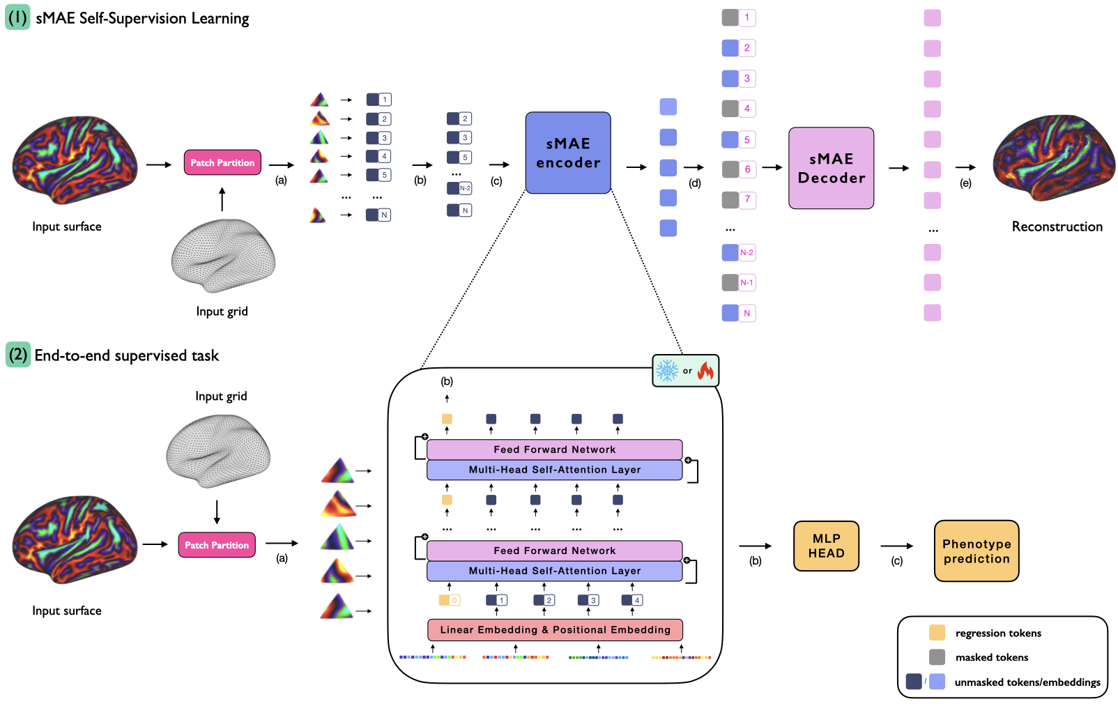
Figure 1: sMAE learning pipeline. The sMAE regime involves masking part of the input token sequence (1.b), before passing the unmasked tokens to the sMAE encoder (SiT-tiny) (1.c). Unmasked token embeddings and a set of mask tokens are then concatenated (1.d) and passed to the decoder to reconstruct the masked patches (1.e). End-to-end finetuning (2) involves extracting the sMAE encoder and performing supervised training for downstream tasks, by finetuning or freezing the entire encoder, alongside the MLP head.

Here, we adopt the SiT architecture [7], which translated the concept of ViTs to sphericalised cortical meshes by representing the cortical surface as a mesh structure on a sphere. Input data $X\in\mathbb{R}^{|V_{6}|\times C}$ ($C$ channels) is represented on a 6th-order icospheric (ico6) tessellation: $I_{6}=(V_{6},F_{6})$, with $|V_{6}|=40962$ vertices and $|F_{6}|=81920$ faces. Surface patching is achieved by tessellating ico6 surfaces according to the regular subdivisions of a low-resolution icosphere, typically ico3 $I_{3}=(V_{3},F_{3})$ ($|F_{3}|=1280$ and $|V_{3}|=642$), see Figure 1.a. This partition leads to a sequence of $|F_{3}|=1280$ non-overlapping triangular patches: $T_{3}=\{t^{1}_{3},t^{2}_{3},..t_{3}^{|F_{3}|}\}$ (with $t^{i}_{3}\subset V_{6};|t^{i}_{3}|=|t_{3}|=45$). Imaging features for each patch are then concatenated across channels, and flattened to produce an initial sequence of tokens: $\hat{\mathcal{X}}=\left[X^{0}_{1},...,X^{0}_{N}\right]\in\mathbb{R}^{N\times(|t_{3}|C)}$, where $N=|F_{3}|$. These are first projected onto a $D-$dimensional sequence using a trainable linear layer. Then, an extra $D$-dimensional token for regression or classification is concatenated ($X^{0}_{0}$) and positional embeddings ($E_{pos\_enc}\in\mathbb{R}^{(N+1)\times D}$) are added to encode patch location into a sequence of tokens such that $\mathcal{X}=\left[X^{0}_{0},...,X^{0}_{N}\right]+E_{pos\_enc}\in\mathbb{R}^{(N+1)\times D}$. In contrast to [7], we adopt positional embeddings in the form of 1D sine-cosine embeddings. Then, this sequence of tokens is processed by the SiT network which consists of $L$ consecutive transformer encoder blocks of Multi-Head Self-Attention (MHSA) and Feed Forward Network (FFN) layers, with residual layers in-between:

$$\mathcal{Z}^{(l)} =\textbf{\emph{MSHA}}(\mathcal{X}^{(l)})+\mathcal{X}^{(l)}$$ (1)

$$\mathcal{X}^{(l+1)} =\textbf{\emph{FFN}}(\mathcal{Z}^{(l)})+\mathcal{Z}^{(l)}$$

$$=\left[X^{(l+1)}_{0},...,X^{(l+1)}_{N}\right]\in\mathbb{R}^{(N+1)\times D}$$

In the last output sequence, the regression token ${X}^{(L)}_{0}$ is used as input to the final Multi-Layer Perceptron (MLP) for prediction (classification or regression).

2.2 Surface Masked AutoEncoder

The Masked AutoEncoder (MAE) [13] frames self-supervision of vision transformers as an image reconstruction problem. During training, a fraction of the input signal is randomly masked out, and the model aims to reconstruct the missing patches.

2.2.1 Pre-training network

Similarly to [13] the sMAE architecture follows an asymmetric encoder-decoder design (Fig 1). The encoder processes only the unmasked tokens of the input sequence, while the decoder receives input at the full resolution of the original embedded sequence. This includes the latent representations of the unmasked tokens and the masked tokens (empty embeddings). In this implementation, the encoder is a SiT-tiny (with $L=12$ transformer encoder layers, with 3 MHSA heads per layer), and the decoder is computationally lighter: built from 1/4 of the number of layers of a SiT-tiny model and the same number of MHSA heads. Finally, a linear layer is applied to project the tokens in the final sequence back into the input patch resolution (Figure 1.e). Here, the decoder is only used for pre-training, whereas the encoder is used for finetuning downstream tasks. Two different types of finetuning were performed: end-to-end finetuning where all encoder layers are retrained following SSL with the MLP head; or partial finetuning, in particular linear probing, where all encoder layers are kept frozen, and only the MLP head is trained.

2.2.2 Reconstruction Task

After adding positional embeddings $E_{pos\_enc}$ to the input sequence $\mathcal{X}$, a set of token indices $J_{mask}$ is randomly sampled to mask a fraction of the input sequence (see Fig 1.b) such that $J=J_{mask}\cup J_{unmasked}$, where $J=\{0,1...,N\}$ and $J_{mask}\cap J_{unmask}=\emptyset$. The sequence of unmasked tokens $\mathcal{X}_{unmasked}=\allowbreak\left\{X^{0}_{i}|i\in J_{unmasked}\right\}$ is first encoded (Fig 1.c); then the output $\mathcal{X}^{(L)}_{unmasked}$ (Eq.1) is concatenated to the set of masked embeddings and the entire sequence is unshuffled, to restore the original token order (Fig 1.d). Fixed positional embeddings $E_{pos\_dec}\in\mathbb{R}^{(N+1)\times D}$ are added to this sequence of embeddings, before passing it to the decoder, which seeks to output a full-resolution reconstruction of the image. Note, the loss (Mean Square Error, MSE) is computed only between the masked patches, following [13].

2.2.3 Masked Patch Prediction

The sMAE methodology is compared to the Masked Patch Prediction (MPP) task, used previously in [7], which in turn was adapted from [9, 8]. It employs an autoencoder architecture that is trained to reconstruct the entire image sequence while corrupting some of the input patches through masking or swapping. Following [9], we corrupt 50% of the input patches randomly: by replacing the patches with a masked (empty) token (40%), using another patch embedding from the sequence at random (5%), or preserving their original embeddings (5%). In contrast to sMAE, the MPP methodology optimises reconstruction by computing the MSE loss for all patches. In this approach, the SiT encoder processes the entire sequence of patches, and the decoder is limited to projecting the last encoder’s sequence to the input patch resolution.

3 Experiments and Results

We evaluate the performance of the sMAE framework for cortical phenotype regression from neonatal cortical surface features from the dHCP under three supervised training schemes: end-to-end finetuning on all data, end-to-end finetuning on a subset of the data, and linear probing on all data.

3.1 Dataset and Tasks

3.1.1 dHCP

Data from the dHCP consists of cortical surface meshes and metrics (sulcal depth, curvature, cortical thickness and T1w/T2w myelination) derived from T1- and T2-weighted magnetic resonance images (MRI) [19]. We use 580 scans from 419 term neonates (born after $37$ weeks gestation) and 111 preterm neonates (born prior to $37$ weeks gestation). 95 preterm neonates were scanned twice, once shortly after birth, and once at term-equivalent age. Phenotype regression was preformed on two tasks: prediction of postmenstrual age (PMA) at scan, and gestational age (GA) at birth. For PMA prediction training data was drawn from the scans of term-born neonates and preterm neonates’ first scans (26.71 to 44.71 weeks PMA) with a train:val:test split of 423:53:54 examples. The GA model predicts the degree of prematurity from the participants’ term-age scans (scans from term neonates and preterm neonate’s second scans) with a split of 411:51:52 examples. In both cases, balanced distribution of examples from each age bin was ensured. For the end-to-end finetuning of PMA with partial data, three subsets of the training data were generated with respectively 10%, 20%, and 50% of the full dHCP training dataset. The distribution of scan age across the full training set was preserved while generating the subsets.

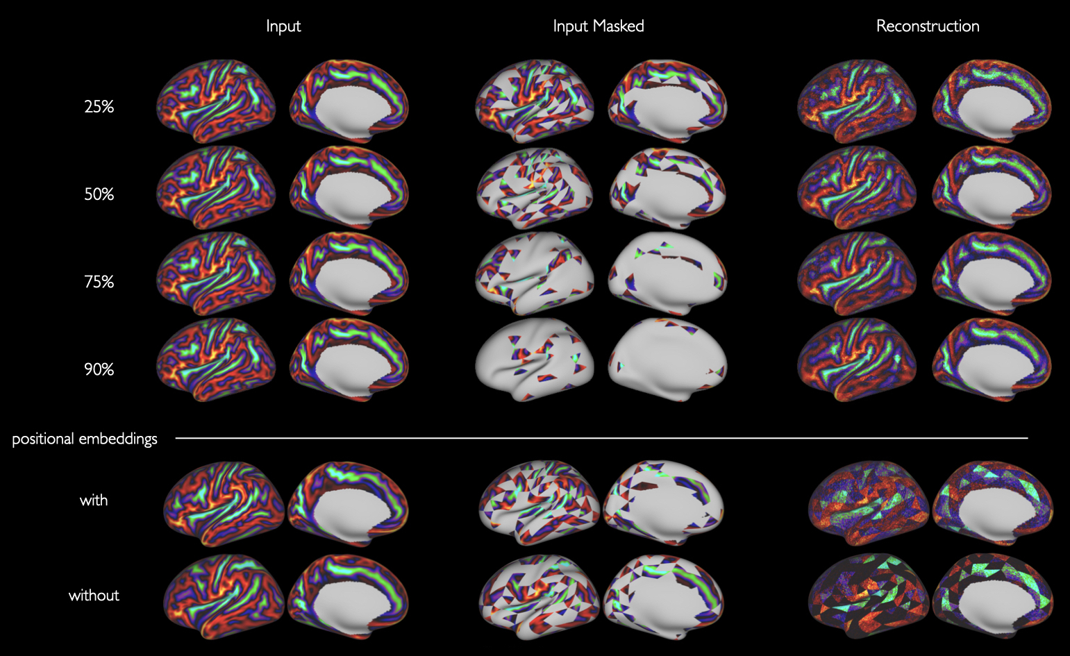
Figure 2: Sulcal depth reconstructions from the surface Masked AutoEncoder (sMAE) trained for different masking ratios (%). Below, we compare the outputs of two sMAE trained with 50% patching with and without using positional embeddings. sMAE networks were trained for a maximum of 100 epochs.

3.1.2 UK Biobank (UKB)

Data collected from 4063 subjects (1896 biological females) aged between 46 and 83 years [20, 1] was also used. In this case, cortical surfaces and metrics (similar to dHCP) were reconstructed using the HCP structural pipeline [12]. We split the dataset into train:val:test sets of respective size 2865:588:610.

Encoder	Pre-training	PMA at Scan		Gestational Age
architecture	method	error $\pm$ std	R2	error $\pm$ std	R2
	None	0.87 $\pm$ 0.08	0.92	1.65 $\pm$ 0.11	0.57
SiT-tiny ico3	MPP	0.66 $\pm$ 0.02	0.95	1.53 $\pm$ 0.07	0.60
	Ours (sMAE)	0.64 $\pm$ 0.03	0.96	1.22 $\pm$ 0.02	0.77

Table 1: Fine-tuning results of PMA and GA under different SSL frameworks: from scratch (None), after MPP and sMAE. Each SiT-tiny encoder is trained three times, averaged test prediction errors and stds are shown in the table.

Masking Ratio	Reconstruction Error	Gestational Age
25%	0.348	1.51 $\pm$ 0.10
50%	0.290	1.35 $\pm$ 0.02
75%	0.301	1.42 $\pm$ 0.04
90%	0.302	1.44 $\pm$ 0.07

Table 2: Masking ratio selection. Reconstruction errors (MSE) on validation set for masked patches only. For each masking ratio configuration, the sMAE encoder was fine-tuned for GA prediction and 200 epochs. Validation prediction errors with stds across three runs are reported.

3.1.3 Training Settings

Prior to training, data normalisation was performed on a per-subject and per-channel basis. Additionally, each channel was clipped to a range of values within $\pm 3$ standard deviations (std). All models were trained on a single RTX 3090 NVIDIA GPU using stochastic gradient descent (SGD) optimization with a momentum of 0.9 and a learning rate of $1e^{-4}$. For the linear probing experiments, the learning rate was reduced to $1e^{-5}$.

3.2 Results

3.2.1 Effect of Masking Ratio

We first evaluate the effect of the masking ratio hyperparameter of the sMAE framework. sMAE networks were trained with different masking ratios (25%, 50%, 75% and 90%) on dHCP data and evaluated for both reconstruction quality and prediction performance in a downstream task (GA regression). Table 2 reports the best MSE reconstruction errors and mean absolute error (referred to as prediction error in the following) on the validation set, averaged across three fine-tuning runs. Figure 2 shows an example of the reconstruction quality for the validation set for each sMAE masking ratio, indicating that sMAE models capture individual cortical features even with high masking ratios, which suggests some capabilities of self-attention to model complex dependencies between brain regions. Overall, the 50% masking ratio offered the best quantitative validation and was used in all following experiments. Such observations are aligned with those in [13], where it was noted that masking a high percentage of patches is necessary to reduce redundancy and create a challenging self-supervisory task which leads to learning more meaningful weights.

3.2.2 Performance on end-to-end finetuning.

We benchmark the use of the sMAE against the MPP for pre-training SiT-tiny models and compare against training models from scratch for 1000 epochs for the tasks of PMA at scan and GA at birth regression. Results in Table 1 show that sMAE on dHCP data improved performance in all cases compared to training from scratch and with an MPP: 26% and 3% respectively (on PMA prediction) and 26% and 20% respectively (GA regression). In addition to performance improvements, a major advantage of using SSL as pre-training for the SiT is the speed gain in the process of training the supervised task. Here, faster convergence is defined as no improvement in validation loss and prediction error for at least 20 consecutive epochs. Figure 3 a) and b) show the validation loss and prediction error across three fine-tuning runs of the sMAE encoder (SiT-tiny) for the task of GA prediction. On average, sMAE pre-training resulted in a 66% faster convergence on GA prediction and 80% on PMA, compared to training from scratch.

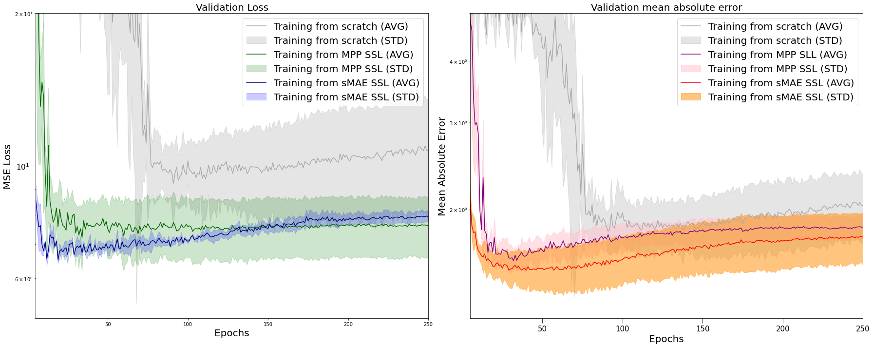
Figure 3: GA prediction results comparing training from scratch, finetuning from MPP and from sMAE. Left: validation loss; Right: validation error. Mean and std performances (across 3 runs) are plotted. The y-axis is shown in log-scale.

3.2.3 Evaluating transfer learning capabilities with sMAE.

To assess the potential of sMAE SSL for transfer learning on smaller datasets, we first investigate the effectiveness of end-to-end fine-tuning, using subsets of the entire dHCP dataset (10%, 20% or 50%). Results are reported for the PMA task in Table 3.a. Remarkably, even with only 20% of the samples for fine-tuning, the model pretrained on dHCP data achieved better results than training from scratch using the entire dataset (Table 1). Pre-training on UKB also benefits the end-to-end finetuning in all dHCP finetuning sizes, compared to training from scratch.

Next, a linear probing experiment was conducted using sMAE models pre-trained either with dHCP or UKB data (referred as sMAE (dHCP) and sMAE (UKB) in Table 3.a and 3.b). In both cases, finetuning is performed by training only the regression head (577 parameters) while keeping all encoder layers frozen, and demonstrates comparable performance to a full SiT-tiny (5M parameters) trained from scratch (Table 3.a).

% dHCP data	None	sMAE (UKB)	sMAE (dHCP)
10%	1.73	1.58	0.84
20%	1.48	1.36	0.76
50%	1.36	0.92	0.66
100%	0.81	0.70	0.61

(a) End-to-end finetuning on different dHCP dataset sizes from scratch (None); or following sMAE pre-training on UKB or dHCP data.

Pre-training (dataset)	Linear Probing
None	1.63
sMAE (UKB)	0.84
sMAE (dHCP)	0.78

(b) In linear probing, only 577 parameters are trained (MLP head). Finetuning is done on all available dHCP training data.

Table 3: Transfer Learning experiments on PMA prediction. In both tables, sMAE (dHCP) and sMAE (UKB) models are pre-trained on 100% of available training data. Best prediction errors on the PMA dHCP test set are reported.

4 Discussion

In conclusion, sMAE SSL pretraining of SiTs demonstrates improved performance relative to MPP pretraining and training from scratch on phenotype regression tasks, suggesting that image reconstruction with masked autoencoders learns robust cortical feature representations that generalise well to downstream tasks. Importantly, findings from finetuning on partial datasets, and linear probing of UKB, suggests that sMAE pre-training could generalise the application of SiTs to much smaller cortical imaging datasets. However, it is worth noting some drop in performance when moving from dHCP to UKB pre-training, which might point to issues of domain shift. Note that while data augmentation techniques were not employed in this study (to assess gains solely from pre-training) incorporating such techniques in future studies could further enhance generalisation performance.

References

- [1] Alfaro-Almagro, F., Jenkinson, M., Bangerter, N.K., Andersson, J.L., Griffanti, L., Douaud, G., Sotiropoulos, S.N., Jbabdi, S., Hernandez-Fernandez, M., Vallee, E., et al.: Image processing and quality control for the first 10,000 brain imaging datasets from uk biobank. Neuroimage 166, 400–424 (2018)
- [2] Azizi, S., Mustafa, B., Ryan, F., Beaver, Z., Freyberg, J., Deaton, J., Loh, A., Karthikesalingam, A., Kornblith, S., Chen, T., Natarajan, V., Norouzi, M.: Big Self-Supervised Models Advance Medical Image Classification (Apr 2021), http://arxiv.org/abs/2101.05224, arXiv:2101.05224 [cs, eess]
- [3] Bello, G.A., Dawes, T.J.W., Duan, J., Biffi, C., de Marvao, A., Howard, L.S.G.E., Gibbs, J.S.R., Wilkins, M.R., Cook, S.A., Rueckert, D., O’Regan, D.P.: Deep-learning cardiac motion analysis for human survival prediction. Nature Machine Intelligence 1(2), 95–104 (feb 2019). https://doi.org/10.1038/s42256-019-0019-2, https://doi.org/10.1038%2Fs42256-019-0019-2
- [4] Bronstein, M.M., Bruna, J., Cohen, T., Veličković, P.: Geometric deep learning: Grids, groups, graphs, geodesics, and gauges (2021). https://doi.org/10.48550/ARXIV.2104.13478, https://arxiv.org/abs/2104.13478
- [5] Caron, M., Touvron, H., Misra, I., Jégou, H., Mairal, J., Bojanowski, P., Joulin, A.: Emerging properties in self-supervised vision transformers (2021). https://doi.org/10.48550/ARXIV.2104.14294, https://arxiv.org/abs/2104.14294
- [6] Chen, L., Bentley, P., Mori, K., Misawa, K., Fujiwara, M., Rueckert, D.: Self-supervised learning for medical image analysis using image context restoration. Medical Image Analysis 58, 101539 (Dec 2019). https://doi.org/10.1016/j.media.2019.101539, https://www.sciencedirect.com/science/article/pii/S1361841518304699
- [7] Dahan, S., Fawaz, A., Williams, L.Z., Yang, C., Coalson, T.S., Glasser, M.F., Edwards, A.D., Rueckert, D., Robinson, E.C.: Surface vision transformers: Attention-based modelling applied to cortical analysis. arXiv preprint arXiv:2203.16414 (2022)
- [8] Devlin, J., Chang, M.W., Lee, K., Toutanova, K.: Bert: Pre-training of deep bidirectional transformers for language understanding (2019)
- [9] Dosovitskiy, A., Beyer, L., Kolesnikov, A., Weissenborn, D., Zhai, X., Unterthiner, T., Dehghani, M., Minderer, M., Heigold, G., Gelly, S., Uszkoreit, J., Houlsby, N.: An image is worth 16x16 words: Transformers for image recognition at scale. CoRR abs/2010.11929 (2020), https://arxiv.org/abs/2010.11929
- [10] Fawaz, A., Williams, L.Z., Alansary, A., Bass, C., Gopinath, K., da Silva, M., Dahan, S., Adamson, C., Alexander, B., Thompson, D., et al.: Benchmarking geometric deep learning for cortical segmentation and neurodevelopmental phenotype prediction. bioRxiv pp. 2021–12 (2021)
- [11] Ghesu, F.C., Georgescu, B., Mansoor, A., Yoo, Y., Neumann, D., Patel, P., Vishwanath, R.S., Balter, J.M., Cao, Y., Grbic, S., Comaniciu, D.: Self-supervised Learning from 100 Million Medical Images (Jan 2022), http://arxiv.org/abs/2201.01283, arXiv:2201.01283 [cs]
- [12] Glasser, M., Sotiropoulos, S., Wilson, J., Coalson, T., Fischl, B., Andersson, J., Xu, J., Jbabdi, S., Webster, M., Polimeni, J., DC, V., Jenkinson, M.: The minimal preprocessing pipelines for the human connectome project. NeuroImage 80, 105 (10 2013). https://doi.org/10.1016/j.neuroimage.2013.04.127
- [13] He, K., Chen, X., Xie, S., Li, Y., Dollár, P., Girshick, R.: Masked autoencoders are scalable vision learners (2021)
- [14] Hou, Z., Liu, X., Cen, Y., Dong, Y., Yang, H., Wang, C., Tang, J.: Graphmae: Self-supervised masked graph autoencoders (2022)
- [15] Kim, B.H., Ye, J.C., Kim, J.J.: Learning dynamic graph representation of brain connectome with spatio-temporal attention (2021). https://doi.org/10.48550/ARXIV.2105.13495, https://arxiv.org/abs/2105.13495
- [16] Krishnan, R., Rajpurkar, P., Topol, E.J.: Self-supervised learning in medicine and healthcare. Nature Biomedical Engineering 6(12), 1346–1352 (Dec 2022). https://doi.org/10.1038/s41551-022-00914-1, https://www.nature.com/articles/s41551-022-00914-1, number: 12 Publisher: Nature Publishing Group
- [17] Liang, Y., Zhao, S., Yu, B., Zhang, J., He, F.: Meshmae: Masked autoencoders for 3d mesh data analysis (2022)
- [18] Ma, Q., Robinson, E.C., Kainz, B., Rueckert, D., Alansary, A.: Pialnn: A fast deep learning framework for cortical pial surface reconstruction (2021). https://doi.org/10.48550/ARXIV.2109.03693, https://arxiv.org/abs/2109.03693
- [19] Makropoulos, A., Robinson, E.C., Schuh, A., Wright, R., Fitzgibbon, S., Bozek, J., Counsell, S.J., Steinweg, J., Vecchiato, K., Passerat-Palmbach, J., Lenz, G., Mortari, F., Tenev, T., Duff, E.P., Bastiani, M., Cordero-Grande, L., Hughes, E., Tusor, N., Tournier, J.D., Hutter, J., Price, A.N., Teixeira, R.P.A., Murgasova, M., Victor, S., Kelly, C., Rutherford, M.A., Smith, S.M., Edwards, A.D., Hajnal, J.V., Jenkinson, M., Rueckert, D.: The Developing Human Connectome Project: A Minimal Processing Pipeline for Neonatal Cortical Surface Reconstruction (apr 2018). https://doi.org/10.1101/125526, https://pubmed.ncbi.nlm.nih.gov/29409960/
- [20] Miller, K.L., Alfaro-Almagro, F., Bangerter, N.K., Thomas, D.L., Yacoub, E., Xu, J., Bartsch, A.J., Jbabdi, S., Sotiropoulos, S.N., Andersson, J.L., et al.: Multimodal population brain imaging in the uk biobank prospective epidemiological study. Nature neuroscience 19(11), 1523–1536 (2016)
- [21] Radford, A., Wu, J., Child, R., Luan, D., Amodei, D., Sutskever, I.: Language models are unsupervised multitask learners (2019)
- [22] Suliman, M.A., Williams, L.Z., Fawaz, A., Robinson, E.C.: A deep-discrete learning framework for spherical surface registration. In: International Conference on Medical Image Computing and Computer-Assisted Intervention. pp. 119–129. Springer (2022)
- [23] Xu, H., Williams, S.E., Williams, M.C., Newby, D.E., Taylor, J., Neji, R., Kunze, K.P., Niederer, S.A., Young, A.A.: Deep learning estimation of three-dimensional left atrial shape from two-chamber and four-chamber cardiac long axis views. European Heart Journal - Cardiovascular Imaging 24(5), 607–615 (02 2023). https://doi.org/10.1093/ehjci/jead010, https://doi.org/10.1093/ehjci/jead010
- [24] Yu, X., Tang, L., Rao, Y., Huang, T., Zhou, J., Lu, J.: Point-bert: Pre-training 3d point cloud transformers with masked point modeling (2022)