$\mathcal{G}^{2}Pxy$: Generative Open-Set Node Classification on Graphs with Proxy Unknowns

Abstract

Node classification is the task of predicting the labels of unlabeled nodes in a graph. State-of-the-art methods based on graph neural networks achieve excellent performance when all labels are available during training. But in real-life, models are often applied on data with new classes, which can lead to massive misclassification and thus significantly degrade performance. Hence, developing open-set classification methods is crucial to determine if a given sample belongs to a known class. Existing methods for open-set node classification generally use transductive learning with part or all of the features of real unseen class nodes to help with open-set classification. In this paper, we propose a novel generative open-set node classification method, i.e., $\mathcal{G}^{2}Pxy$, which follows a stricter inductive learning setting where no information about unknown classes is available during training and validation. Two kinds of proxy unknown nodes, inter-class unknown proxies and external unknown proxies are generated via mixup to efficiently anticipate the distribution of novel classes. Using the generated proxies, a closed-set classifier can be transformed into an open-set one, by augmenting it with an extra proxy classifier. Under the constraints of both cross entropy loss and complement entropy loss, $\mathcal{G}^{2}Pxy$ achieves superior effectiveness for unknown class detection and known class classification, which is validated by experiments on benchmark graph datasets. Moreover, $\mathcal{G}^{2}Pxy$ does not have specific requirement on the GNN architecture and shows good generalizations.

1 Introduction

Node classification is the task of assigning labels (categories) to unlabeled graph nodes. This task has many important applications such as traffic state prediction Zheng et al. (2020), and completing user profiles in social networks Wong et al. (2021). Graph Neural Network (GNN) based methods Zhu et al. (2022); Liu et al. (2021) achieve state-of-the-art performance for this problem. However, they generally assume that the full set of labels (known classes) is available for training. Unfortunately, this assumption does not hold in many practical scenarios because of unforeseen factors. For instance, a trained GNN may be applied on samples from a research social network where researchers may have published in new conferences that were unseen in training. When facing samples of unknown classes, typical GNN methods Kipf and Welling (2017); Veličković et al. (2018); Hamilton et al. (2017) will incorrectly label nodes using known classes, which can considerably degrade performance. Hence, building models that can classify samples from known classes and reject samples from unknown classes is a key issue, which is known as the open set classification problem.

Recent techniques that have been designed to address the open-set node classification problem Wu et al. (2021) presume that a model will be more confident in its predictions for closed-set samples than for open-set samples. Relying on this assumption, a threshold is applied on a model’s confidence scores to separate unknown samples from known ones. Though this approach is intuitive Hendrycks and Gimpel (2017), it often fails because deep neural networks tend to be over-confident in input samples and may output high confidence scores even for an unknown input Hein et al. (2019); Guo et al. (2017); Bendale and Boult (2016); Scheirer et al. (2012). Moreover, finding an optimal threshold to separate known from unknown classes is hard and time-consuming Perera et al. (2020); Ge et al. (2017).

Another critical challenge for open-set classification is the lack of open-set data. It is hard to collect open-set data due to the very large diversity. However, most of the prior solutions Wu et al. (2020) follow a transductive learning approach, i.e., suppose that part or all of the features of the real unseen class samples can be observed and used to help with open-set learning. This setting is not suitable for most real-world applications. To alleviate this issue, several studies on image classification have attempted to estimate the distribution of unknown classes and calibrate a network’s confidence. For example, G-OpenMax Ge et al. (2017) utilizes a GAN to generate unknown samples for training an image classifier. Neal et al. Neal et al. (2018) introduced a counterfactual image generation method to produce image samples lying between decision boundaries through GANs. Perera et al. Perera et al. (2020) combined self-supervision and a generative model to enhance the optimal closed-set features and to effectively identify open-set samples. PROSER Zhou et al. (2021) learns placeholders to prepare for unknown classes by allocating placeholders for both data and classifier, which yields high disparity.

Motivated by the above studies, we propose a novel Generative open-set node classification method on Graphs with Proxy unknowns ($\mathcal{G}^{2}Pxy$ for short). Under the constraints of not being able to obtain open-set data, $\mathcal{G}^{2}Pxy$ first generates pseudo unknown class nodes (unknown proxies) via mixup Verma et al. (2019); Han et al. (2022), to mimic the distribution of unknown classes using only the closed-set graph for learning. Two kinds of proxy unknown nodes, inter-class unknown proxies and external unknown proxies, are generated. Using the generated proxies, a closed-set classifier can be transformed into an open-set one, by augmenting it with an extra proxy classifier. The whole model is optimized under the supervision of cross entropy and tailored complement entropy loss Chen et al. (2018) together, and can then adaptively perform class-specific classification and detection during testing. Moreover, $\mathcal{G}^{2}Pxy$ can be adopted by different kinds of GNNs and shows good generalizations. The contributions of this paper are summarized as follows:

• A novel method $\mathcal{G}^{2}Pxy$ for open-set node classification is proposed with efficient unknown proxy generation and open-set classifier learning, under the constraint of both cross entropy and complement entropy loss. To the best of our knowledge, $\mathcal{G}^{2}Pxy$ is the first generative method for open-set graph learning.

• No open-set data (samples of unknown classes or any side information of unknown classes) is required during training and validation. $\mathcal{G}^{2}Pxy$ has an explicit classifier for unknown and does not require tuning a threshold.

• $\mathcal{G}^{2}Pxy$ does not have specific requirement on the GNN architecture, and shows good generalizations. Using mixup as the generative method also ensures the efficiency, due to the acceptable extra computation cost.

• Experiments on benchmark graph datasets demonstrate the good performance of $\mathcal{G}^{2}Pxy$.

2 Problem Definition & Preliminary

This paper focuses on the node classification problem for a graph. Consider a graph denoted as $G=(V,E,X)$, where $V=\{v_{i}|{i=1,\ldots,N}\}$ is a set of $N$ nodes in the graph. $E=\{e_{i,j}|i,j=1,\ldots,N.$ $i\neq j\}$ is a set of edges between pairs of nodes $v_{i}$ and $v_{j}$. $X\in\mathbb{R}^{N\times d}$ denotes the feature matrix of nodes, and $d$ is the dimension of node features. $x_{i}\in X$ indicates the feature vector associated with each node $v_{i}$. The topological structure of $G$ is represented as an adjacency matrix $A\in\mathbb{R}^{N\times N}$, where $A_{i,j}=1$ if the nodes $v_{i}$ and $v_{j}$ are connected, i.e., $\exists e_{i,j}\in E$, otherwise $A_{i,j}=0$. $Y\in\mathbb{R}^{N\times C}$ is the label matrix of $G$, where $C$ is the already-known node classes. If node $v_{i}\in V$ is associated with a label $c$, $y_{i,c}=1$, otherwise, $y_{i,c}=0$.

For a typical closed-set node classification problem, a GNN encoder $f_{\theta_{g}}$ takes node features $X$ and adjacency matrix $A$ as input, aggregates the neighborhood information and outputs representations. Then, a classifier $f_{\theta_{c}}$ is used to classify the nodes into $C$ already-known classes. The GNN encoder and the classifier are optimized to minimize the expected risk  Yu et al. (2017) in Eq. (1), with the assumption that test data $\mathcal{D}_{te}$ and train data $\mathcal{D}_{tr}$ share the same feature space and label space, i.e.,

$$f^{*}=arg\min_{f\in\mathcal{H}}\mathbb{E}_{(x,y)\sim\mathcal{D}_{te}}\mathbb{I}(y\neq f(\theta_{g},\theta_{c};x,A))$$ (1)

where $\mathcal{H}$ is the hypothesis space, $\mathbb{I}(\cdot)$ is the indicator function which outputs 1 if the expression holds and 0 otherwise. Generally, it can be optimized with cross-entropy to discriminate between known classes.

In open-set node classification problem, given a graph $G=(V,E,X)$, $\mathcal{D}_{tr}=(X,Y)$ denotes the train nodes. $\overline{\mathcal{D}}_{te}=(X_{te},Y_{te})$ is the test nodes, where $X_{te}=S\cup U$, $Y_{te}=\{1,\ldots,C,C+1,\ldots\}$. $S$ is the set of nodes that belong to seen classes that already appeared in $\mathcal{D}_{tr}$ and $U$ is the set of nodes that do not belong to any seen class (i.e., unknown class nodes). Open-set node classification aims to learn a $(C+1)$-$class$ classifier $f_{\overline{\theta}_{c}}$ that $f(\theta_{g},\overline{\theta}_{c};X_{te},\overline{A}):\{X_{te},\overline{A}\}\rightarrow\overline{\mathcal{Y}}$, $\overline{\mathcal{Y}}=\{1,\ldots,C,unknown\}$, with the minimization of the expected risk Yu et al. (2017):

$$\overline{f}^{*}=arg\min_{f\in\mathcal{H}}\mathbb{E}_{(x,y)\sim\mathcal{\overline{D}}_{te}}\mathbb{I}(y\neq f(\theta_{g},\overline{\theta}_{c};x,\overline{A}))$$ (2)

where $\overline{A}$ is the adjacency matrix for $X_{te}$. The predicted class $unknown\in\overline{\mathcal{Y}}$ contains a group of novel categories, which may contain more than one class. Thus, the overall risk aims to classify known classes while also detecting the samples from unseen categories as class $unknown$.

From close-set to open-set classifier, an intuitive way is thresholding Hendrycks and Gimpel (2017). Taking the max output probability as confidence score, i.e., $conf=max_{c=1,\ldots,C}f_{c}(x,A)$, it assumes the model is more confident in closed-set instances than open-set ones. Then we can extend a closed-set classifier by

$$\hat{y}_{i}=\left\{\begin{aligned} &\arg\max_{c=1,\ldots C}f_{c}(x_{i},A),\ conf>\tau\\ &unknown,\ \ \ \ \ \ \ \ \ \ \ \ otherwise.\end{aligned}\right.$$ (3)

where $\tau$ is a threshold. However, due to the overconfidence phenomena of deep neural networks, the output confidence of known and unknown is both high Bendale and Boult (2016). As a result, tuning a threshold that well separates known from unknown is hard and time-consuming.

Differently, the approach presented in this paper utilizes an additional proxy classifier to detect the unknown class nodes, with well-designed generated unknown proxies to facilitate the model training. There are advantages of adding a class instead of optimizing a threshold as in previous methods Shu et al. (2017); Wu et al. (2020); Bendale and Boult (2016), since it does not require real open-set samples in validation and also eliminates the difficulty of tuning the threshold.

3 Methodology

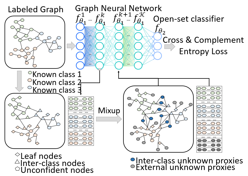
Figure 1: An overview of $\mathcal{G}^{2}Pxy$. Firstly, a graph with labeled nodes is input into the GNN model $f_{\theta_{1}}$. Inter-class and external unknown proxies are created in the middle of GNN (at the $k$-th layer). Then the generated proxies and the original training data are input into the rest of the neural network to learn an open-set classifier $f_{\theta_{2}}$, under the constraint of cross entropy and complement entropy loss.

Facing the difficulty of closed-set classifier calibration, we need proxy unknown nodes to foresee the distribution of unknown classes and prepare the open-set model for novel classes.

The overall framework of $\mathcal{G}^{2}Pxy$ is introduced in Fig. 1. Specifically, a GNN encoder $f_{\theta_{1}}$ takes node features $X$ and adjacency matrix $A$ as input, aggregates the neighborhood information and outputs representation $h_{i}^{k}$ for each node $v_{i}$ in its $k$-th layer, $k=1,\ldots,\mathcal{K}$. $\mathcal{K}$ is the total number of layers. Thus, in the $k$-th layer, for node $v_{i}$, the GNN encoder aggregates neighbor information from the $k$-$1$ layer into a neighborhood representation:

$$h_{i}^{k}=f^{k}(\theta_{1};h_{i}^{k-1},h_{j}^{k-1},j\in\mathcal{N}_{i})$$ (4)

where $h_{i}^{k}\in\mathbb{R}^{d_{k}}$ is the hidden representation at the $k$-th layer, $\mathcal{N}_{i}$ is the neighborhood of node $v_{i}$ and $h^{0}=X$.

Meanwhile, we mimic novel patterns by generating proxy unknown nodes through manifold mixup Verma et al. (2019); Han et al. (2022). Targeted node pairs are selected and mixed up at the middle layer of the GNN, and two kinds of proxies are created: inter-class unknown proxies that separate known classes from each other and external unknown proxies that separate known from unknown. Generated proxies and original known class nodes are input into the remaining layers together to learn discriminative representations. Then, a classifier $f_{\theta_{2}}$ is learned to classify the nodes into $C+1$ classes, achieving open-set node classification.

To conclude, the proposed $\mathcal{G}^{2}Pxy$ method consists of two main modules: 1) a proxy node generation module to create proxy unknown class nodes; 2) an open-set classifier learning module to guarantee the classification of known classes and the rejection of the unknown class. We introduce them in details.

3.1 Proxy Node Generation

As out-of-distribution nodes are unavailable during training, we propose an effective way of generating proxy unknown nodes, which are designed to be located at the boundaries between different classes. These nodes are utilized in the learning process to supervise and tell apart unknown nodes from known ones. Specifically, two different kinds of proxies are produced, inter-class unknown proxies and external unknown proxies. We adopt manifold mixup Verma et al. (2019) as our generation method, due to its efficiency and good interpretability  Han et al. (2022).

3.1.1 Inter-Class Unknown Proxies

For a well-trained classifier, features of nodes that belong to the same categories are close to each other, while those from different classes are distant. Ideally, clear boundaries separate the different classes. Since nodes whose features are close to the boundaries are more likely to be less representative to their own classes, we decided to generate proxy unknowns using nodes near the boundary regions. Thus, samples that belong to different classes but are close to each other are ideal node pairs for proxy generation, i.e., node pairs where the two nodes are in different classes but have an edge between them. In details, given two connected nodes from different categories, i.e., $\{(x_{i},y_{i}),(x_{j},y_{j})\}$, where $y_{i}\neq y_{j}$ and $a_{ij}=1$, their embeddings in the $k$-th layer are $h_{i}^{k}$ and $h_{j}^{k}$, obtained by giving the graph to the network $f_{\theta_{1}}^{1\sim k}$. The inter-class unknown proxy $(\tilde{x}_{i},\tilde{y}_{i})$ are calculated by Eq. (5).

$$\left\{\begin{aligned} &\tilde{x}_{i}=\alpha h_{i}^{k}(\theta_{1};x_{i},A)+\left(1-\alpha\right)h_{j}^{k}\left(\theta_{1};x_{j},A\right)\\ &\tilde{y}_{i}=C+1.\end{aligned}\right.$$ (5)

where $\alpha\in\left[0,1\right]$ is randomly sampled from a Beta distribution and the value of $\alpha$ is around $0.5$. $\tilde{y}_{i}=C+1$ is the category index of $\tilde{x}_{i}$, indicating it belongs to the unknown class. Two edges between $(x_{i},\tilde{x}_{i})$ and $(x_{j},\tilde{x}_{i})$ are also added into the graph. We denote the set of generated inter-class proxies samples as $X_{int}$. The purpose of $X_{int}$ is to simulate the distribution of unknown class nodes that exist between known classes. The mixed hidden representation $\tilde{x}_{i}$ is then passed to $f_{\theta_{1}}^{k+1\sim\mathcal{K}}$ to yield the final representation $\tilde{h}_{i}^{\mathcal{K}}=f_{\theta_{1}}^{\mathcal{K}}(\tilde{x}_{i})$.

3.1.2 External Unknown Proxies

Besides the inter-class unknown proxies, external unknown proxies are further generated to mimic the unknown distributions at the periphery. We use the peripheral nodes from each known class and their corresponding class center to generate the external unknown proxies.

Specifically, the peripheral nodes are selected according to two rules. Rule 1 is to select the leaf nodes of known classes, i.e., $x_{i}\in X_{tr},\ s.t.\ \sum_{j}A_{i,j}=1$. Rule 2 is to collect the nodes with low classification confidence, i.e., the nodes which have the top $T$ least confident scores are selected in each known class. In this way, both structure-based and semantic-based peripheral nodes are picked out. We record the set of peripheral nodes as $X_{per}$.

Moreover, the embedding of class centers in the $k$-th layer can be calculated according to the ground-truth annotations following Eq. (6):

$$h_{(c)}^{k}=\frac{1}{|X^{c}|}\sum_{x_{i}\in X^{c}}h_{i}^{k}(\theta_{1};x_{i},A),c=1,\ldots,C.$$ (6)

where $X^{c}$ denotes the nodes annotated with the class label $c$.

Then, the manifold mixup is applied on peripheral nodes and their corresponding reversed class centers $\{(x_{i},y_{i}),(x_{(y_{i})},y_{i}),x_{i}\in X_{per},y_{i}\in\{1,\ldots,C\}\}$ to obtain the external unknown proxies in the $k$-th layer, i.e.,

$$\left\{\begin{aligned} &\tilde{x}_{i}=h_{i}^{k}(\theta_{1};x_{i},A)+\alpha(-h_{(y_{i})}^{k})\\ &\tilde{y}_{i}=C+1.\end{aligned}\right.$$ (7)

where $\alpha>0$ is a hyperparameter to control the distance between the generated samples and the existing known class samples. Edges between $(x_{i},\tilde{x}_{i}),x_{i}\in X_{per}$ are also added into the graph. We denote the set of generated external unknown proxies as $X_{ext}$.

3.2 Open-Set Classifier Learning

To handle the diverse compositions of known-unknown categories, it is necessary to extract invariant information from the known and unknown classes. Thus, the backbone GNN network $f_{\theta_{1}}$ is shared by the $C+1$ classes to learn class distributions and node representations.

Further, to calibrate closed-set (known classes) classifier to open-set classifier, an extra category is added to the last classification layer for unknown prediction. Suppose that the weights of the closed-set classifier is $w_{close}\in\mathbf{R}^{d_{\mathcal{K}}\times C}$ where $d_{\mathcal{K}}$ is the dimension of the embeddings in the last layer of GNN, the open-set classifier is the combination of the closed-set classifier and the proxy classifier, i.e., ${\theta_{2}}=[w_{close},w_{proxy}]\in\mathbf{R}^{d_{\mathcal{K}}\times(C+1)}$, where $w_{proxy}\in\mathbf{R}^{d_{\mathcal{K}}\times 1}$ is the weights w.r.t. the proxy classifier. Here, the bias term is omitted for simplicity. Then, the integrated classifier is trained with the original known class samples and the generated proxy samples, i.e., $\overline{\mathcal{D}}_{tr}=\mathcal{D}_{tr}\cup(X_{pxy},Y_{C+1})$, $X_{pxy}=X_{int}\cup X_{ext}$, with the cross entropy loss in Eq. (8):

$$l_{1}=\sum_{(x_{i},y_{i})\in{\mathcal{D}}_{tr}}l_{CrE}(\hat{y}_{i},y_{i})+\lambda_{1}\sum_{x_{i}\in{X_{pxy}}}l_{CrE}(\hat{y}_{i},C+1)$$ (8)

where $\hat{y}_{i}=softmax(f_{\theta_{2}}(f_{\theta_{1}}(x_{i})))$ is the output vector of the open-set classifier for the input node $x_{i}$. $l_{CrE}$ denotes the cross entropy loss, i.e., $l_{CrE}(\hat{y}_{i},y_{i})=-y_{i}\log\hat{y}_{i}$.

Though the cross-entropy loss in Eq. (8) exploits mostly the information from the ground-truth class for maximizing data likelihood, the influence from complement classes (i.e., incorrect classes) has been largely ignored Chen et al. (2018). Thus, we further adopt complement entropy Chen et al. (2018) to complement the softmax cross entropy by neutralizing the effects of complement classes.

The complement entropy loss $L_{CoE}$ is defined as the average of sample-wise entropies over complement classes, i.e.,

$$l_{CoE}=-\sum_{c=1,c\neq y_{i}}^{C+1}\frac{\hat{y}_{i,c}}{1-\hat{y}_{i,y_{i}}}\log\frac{\hat{y}_{i,c}}{1-\hat{y}_{i,y_{i}}},\forall(x_{i},y_{i})\in\overline{D}_{tr}$$ (9)

where $\hat{y}_{i,c}$ denotes the predicted probability of node $x_{i}$ belonging to class $c$.

For the needs of the generative open-set classification method $\mathcal{G}^{2}Pxy$, we further modify the above complement entropy according to the data distribution so that it better fits the task. Specifically, for generated unknown proxies, we minimize their original complement entropy, i.e., minimize the average of entropy over the $C$ known classes, since the generated proxies could be adjacent to any of the known class. For the known class nodes, they are mostly adjacent to the generated proxies, i.e., the $C+1$ class, thus we push the proxy classifier to output the second-largest probability for nodes from known classes. According to this consideration, we propose a tailored complement entropy loss for $\mathcal{G}^{2}Pxy$ as follows:

$$l_{2}=\sum_{(x_{i},y_{i})\in{\mathcal{D}}_{tr}}l_{CrE}(\hat{y}_{i}/y_{i},C+1)+\sum_{x_{i}\in{X_{pxy}}}l_{CoE}(\hat{y}_{i},y_{i})$$ (10)

where $\hat{y}_{i}/y_{i}$ represents the prediction logits after removing the probability of its ground-truth label. The first term helps to reduce the misclassification of known class nodes for other known classes. It is believed that with the help of loss in Eq. (10), the open-world classifier $f_{\theta_{2}}$ can classify nodes of known classes to their real categories, and use the proxy classifier to set an appropriate boundary to tell apart the known and the unknown. Finally, the total loss of $\mathcal{G}^{2}Pxy$ is a combination of cross entropy and the tailored complement entropy loss, i.e.,

$$l_{total}=l_{1}+\lambda_{2}l_{2}$$ (11)

where $\lambda_{2}>0$ is the hyperparameter to balance these two losses.

In the test phase, the well learned open-set classifier will be applied to a test node $x_{i}\in\overline{\mathcal{D}}_{te}$, and outputs $C+1$ probabilities $\hat{y}_{i}\in\mathbb{R}^{(C+1)\times 1}$. We choose the largest probability and give the related class label as prediction. Thus, $x_{i}$ will be detected as unknown class sample if the predicted label is $C+1$.

4 Experiments

Experiments were conducted to validate the performance of $\mathcal{G}^{2}Pxy$. These experiments include: open-set node classification comparison, ablation study, and use case. Codes are available online.

Datasets.

Experiments to evaluate the performance for open-set node classification were mainly carried out on four benchmark graph datasets Wu et al. (2020); Zhu et al. (2022), namely Cora, Citeseer, DBLP, PubMed, which are widely used citation network datasets. Statistics are presented in Table 1.

Dataset	Nodes	Edges	Features	Labels
Cora	2708	5429	1433	7
Citeseer	3312	4732	3703	6
DBLP	17716	105734	1639	4
PubMed	19717	44325	500	3

Table 1: Statistics of the experimental datasets.

Metrics.

Accuracy and Macro-F1 are used for performance evaluation.

Implementation Details.

Generally, $\mathcal{G}^{2}Pxy$ adopts GCN Kipf and Welling (2017) as the backbone neural network for experimental evaluation unless otherwise specified. The GCN is configured with two hidden GCN layers in the dimensions of 512 and 128, followed by an additional multilayer perceptron layer of size 64. $\mathcal{G}^{2}Pxy$ is implemented with PyTorch and the networks are optimized using stochastic gradient descent with a learning rate of $1e^{-3}$. The balance parameters $\lambda_{1}$ and $\lambda_{2}$ are chosen by a grid search in the interval from $10^{-2}$ to $10^{2}$ with a step size of $10^{1}$.

The baseline methods are evaluated according to the instructions reported in the original papers with the same parameter configuration unless otherwise specified, and the best results are selected. For each experiment, the baselines and the proposed method were applied using the same training, validation, and testing datasets. The hyperparameters were tuned to get the best performance on the validation set.

All the experiments were conducted on a workstation equipped with an Intel(R) Xeon(R) Gold 6226R CPU and an Nvidia A100.

Test Settings.

Compared to existing studies focusing on open-set classification Wu et al. (2021); Tang et al. (2021); Wang et al. (2020), the evaluation framework is extended. Two kinds of open-set classification evaluations were conducted to consider short or long distances between known classes and unknown classes, i.e., near open-set classification and far open-set classification. Besides, a discussion is provided of different settings in terms of the availability of side information of unknown class samples during training and validation, i.e., the inductive learning setting and the transductive learning setting.

Specifically, in the near open-set classification experiment, for each dataset, the data of several classes were held out as the unknown classes for testing and the remaining classes were considered as the known classes. $70\%$ of the known class nodes were sampled for training, $10\%$ for validation and $20\%$ for testing. In the far open-set classification experiment, nodes from other datasets were used as unknown class samples for testing, instead of the nodes from the same dataset used in training. In experiments with inductive learning setting, there is not any information about the real unknown class (such as the features $x_{i}$ or side information of unknown classes) used during training or evaluation, while under the transductive learning setting, the whole graph (including unlabeled real unknown class nodes) are input during model training or validation.

Baselines.

The following methods are used as the baselines for the open-set classification comparison.

• GCN_soft: GCN Kipf and Welling (2017) is adopted for graph learning, where a softmax layer is used as the final output layer. It has no capability of recognizing the unknown classes.

• GCN_sig: This baseline replaces the softmax layer of GCN with multiple 1-vs-rest of sigmoids as the final output layer, which still does not have the capability of rejecting the unknown classes.

• GCN_soft_$\tau$: Based on GCN_soft, a probability threshold chosen in $\{0.1,0.2,\ldots,0.9\}$ is used for the classification of each class .

• GCN_sig_$\tau$: Similar to GCN_soft_$\tau$, a threshold is combined to GCN_sig.

• GCN_Opmax: Openmax Bendale and Boult (2016) is an open-set recognition model based on “activation vectors”. Extreme value distribution is used to calibrate softmax scores to Openmax scores, which are then used for open-set classification.

• GCN_DOC: DOC Shu et al. (2017) is an open-world classification method for text classification. It uses multiple 1-vs-rest of sigmoids as the final output layer and defines an automatic threshold setting mechanism. GCN is combined with DOC to allow comparison with the proposed model.

• GCN_PROSER: PROSER Zhou et al. (2021) is a novel and highly effective open-set recognition method used in the field of image processing. We paired it with GCN for graph-based comparison.

• OpenWGL: OpenWGL Wu et al. (2020) employs an uncertainty loss in the form of graph reconstruction loss on unlabeled data and using an adaptive threshold to detect the unknown class samples.

Methods	Cora		Citeseer		DBLP		Pubmed
	Acc	F1	Acc	F1	Acc	F1	Acc	F1
GCN_soft	70.6	67.6	44.6	38.9	63.8	59.2	28.9	29.9
GCN_sig	69.2	64.7	45.3	44.5	63.5	58.7	28.9	29.8
GCN_soft_$\tau$	73.6	73.8	57.3	54.5	65.0	62.4	49.7	48.6
GCN_sig_$\tau$	79.7	80.1	62.1	54.6	69.2	68.2	45.1	46.0
GCN_Opmax	74.6	75.1	56.2	54.5	67.2	67.2	49.1	48.7
GCN_DOC	77.8	78.1	66.0	56.7	69.9	69.2	45.6	46.2
GCN_PROSER	83.2	83.7	73.7	63.6	71.7	72.6	71.0	58.4
OpenWGL	78.1	78.9	64.1	60.8	71.4	72.2	65.3	63.4
$\mathcal{G}^{2}Pxy$	84.3	84.8	75.5	71.0	77.3	79.0	73.7	70.2

Table 2: Near open-set classification on four citation network datasets with one unknown class (u=1) in the inductive learning setting. The Numbers reported are all percentage (%).

Methods	Cora		Citeseer		DBLP		Pubmed
	Acc	F1	Acc	F1	Acc	F1	Acc	F1
GCN_soft	70.8	68.2	44.7	38.9	62.9	57.0	29.2	29.7
GCN_sig	68.8	64.5	44.6	40.1	63.4	59.2	29.0	29.5
GCN_soft_t	78.1	78.9	67.3	57.0	67.3	67.7	68.9	27.2
GCN_sig_t	78.3	78.5	65.4	55.3	71.4	71.5	69.0	27.2
GCN_Opmax	77.2	76.9	57.5	56.7	69.0	70.6	55.0	52.1
GCN_DOC	77.3	77.9	65.1	55.3	71.7	72.0	68.4	34.2
GCN_PROSER	84.7	83.6	74.3	66.6	75.3	71.6	72.8	60.8
OpenWGL	83.3	83.5	70.0	65.4	74.3	74.2	71.2	68.0
$\mathcal{G}^{2}Pxy$	90.7	89.7	76.3	71.8	77.5	79.5	78.0	73.4

Table 3: Near open-set classification on four citation network datasets with one unknown class (u=1) under in the transductive learning setting. Numbers reported are all percentage (%).

Methods	Cora		Citeseer		DBLP		Pubmed		Average
	ind	ood	ind	ood	ind	ood	ind	ood	ind	ood	overall
GCN_soft	89.7	00.0	71.8	00.0	92.9	00.0	93.2	00.0	86.9	00.0	52.0
GCN_sig	87.8	00.0	73.0	00.0	92.5	00.0	93.0	00.0	86.6	00.0	51.7
GCN_soft_$\tau$	87.2	23.3	61.4	50.5	85.6	19.2	70.4	40.3	76.2	33.3	61.4
GCN_sig_$\tau$	85.6	57.9	67.1	53.8	79.9	45.8	78.1	30.2	77.7	47.0	64.0
GCN_Opmax	86.6	30.0	60.4	49.4	85.4	27.6	73.4	38.1	76.4	36.3	61.8
GCN_DOC	84.0	54.9	67.7	63.2	79.8	48.1	78.8	30.7	77.6	49.2	64.8
GCN_PROSER	83.2	82.7	72.5	76.0	78.2	58.0	78.0	70.2	78.0	71.7	74.9
OpenWGL	83.4	58.6	66.4	59.9	76.6	60.0	87.9	55.2	78.6	58.4	69.7
$\mathcal{G}^{2}Pxy$	83.8	86.5	73.6	78.7	85.1	60.3	87.6	67.5	82.5	73.3	77.7

Table 4: Detailed classification accuracy in terms of known classes ( in-distribution, ind) and unknown classes (out-of-distribution, ood) for near open-set classification on four datasets with one unknown class under inductive learning. Numbers reported are all percentage (%).

4.1 Open-Set Node Classification Comparison

Since real-world scenarios are complex, where seen and unseen differs in diverse tasks, we evaluate our model from two aspects: near open-set classification, and far open-set classification.

4.1.1 Near Open-Set Classification

Table 2 and 3 list the accuracy and macro-F1 scores of the methods for the near open-set node classification task, where the last class of each dataset is set as the unknown class (i.e. u=1) and the remaining classes are used to train the model. The results in Table 2 were obtained under the inductive learning setting, where there is no side information about the real unknown class samples available during training or validation. The results in Table 3 are obtained under the transductive learning setting, i.e., the features of unknown class nodes are used to facilitate the model training or validation.

It is observed from these results that $\mathcal{G}^{2}Pxy$ outperforms the baselines on the datasets under both the inductive learning and transductive learning settings. This shows that $\mathcal{G}^{2}Pxy$ can better differentiate between a known class and an unknown class, though they are similar to each other. Specifically, $\mathcal{G}^{2}Pxy$ achieves an average of 3.70% improvement over the second-best method (GCN_PROSER) in terms of accuracy, and an average of 9.60% improvement in terms of F1 score on the four datasets, under the inductive learning setting. Also, $\mathcal{G}^{2}Pxy$ achieves 5.01% and 11.25% improvements on average in terms of accuracy and F1 on the four datasets under the transductive learning setting, respectively. Furthermore, by comparing Table 2 and Table 3, it is observed that the involving of real unknown class information during training or validation benefits the model, which is reasonable.

Besides, we show the detailed classification accuracy in terms of known classes (i.e. in-distribution classification, ind for short) and unknown classes (i.e. out-of-distribution classification, ood for short) respectively, in Table 4. The experiment was conducted under the same setting of Table 2. It shows that in order to gain the ability of unknown class detection, there is a slight decrease in the performance of known class classification, i.e. from 86.9% to 82.5% on average, comparing $\mathcal{G}^{2}Pxy$ to closed-set classification method GCN_soft. However, the unknown class detection accuracy is improved from 0% to 73.3% on average, which is remarkable. Compared to other open-set classification methods, such as the globally second best method GCN_PROSER, the average performance of unknown-class node detection is improved from 71.7% to 73.3% while the performance of the known-class classification still gain a certain increase from 78.0% to 82.5% on average.

4.1.2 Far Open-Set Classification

Following the protocol defined in Perera et al. (2020), the models are trained and validated by all training and validation instances of the original dataset (in-distribution data, IND data). While for testing, instances from another dataset are augmented to the original test set as open-set classes (Out-of-distribution data, OOD data). Specifically, three experiments were designed: Cora_Citeseer(i.e., Core as IND data and Citeseer as OOD data); Citeseer_DBLP (Citeseer as IND, DBLP as OOD), and DBLP_Pubmed (DBLP as IND, Pubmed as OOD), to evaluate the performance of the methods for the far open-set classification task. The known-unknown ratio is 1:1 by setting the number of test examples from the OOD dataset to the same number as in the IND dataset.

The results for far open-set classification are shown in Table 5. It is found that $\mathcal{G}^{2}Pxy$ can handle far out-of-distribution classes from diverse inputs and achieve a large performance improvement over state-of-the-art method GCN_PROSER. Surprisingly, the simple thresholding approach of GCN_soft_$\tau$ achieves comparable performance with $\mathcal{G}^{2}Pxy$. This inspires us to combine the generative methods with discriminative methods for far open-set classification in future work.

Methods	Cora_Citeseer		Citeseer_DBLP		DBLP_PubMed
	Acc	F1	Acc	F1	Acc	F1
GCN_soft	43.0	58.9	38.4	42.5	41.9	53.7
GCN_sig	41.6	57.5	36.3	42.1	41.6	45.2
GCN_soft_$\tau$	81.2	77.6	86.2	71.1	85.0	75.6
GCN_sig_$\tau$	69.4	51.8	68.7	48.0	79.8	69.1
GCN_Opmax	56.2	55.1	69.6	60.3	69.6	58.7
GCN_DOC	69.4	57.8	75.5	62.3	78.0	70.7
GCN_PROSER	78.5	79.1	81.5	66.4	78.6	69.0
OpenWGL	80.6	76.7	44.6	11.9	84.6	70.7
$\mathcal{G}^{2}Pxy$	81.3	80.5	87.5	74.4	86.5	72.3

Table 5: Accuracy and macro-F1 for far open-set classification on benchmark datasets. Numbers reported are all percentage (%).

4.2 Ablation Study

Methods	Cora		Citeseer		DBLP		Pubmed
	Acc	F1	Acc	F1	Acc	F1	Acc	F1
$\mathcal{G}^{2}Pxy$_$\tau$	79.6	80.5	71.4	62.8	67.1	67.1	70.0	56.5
$\mathcal{G}^{2}Pxy\_$int	84.2	84.7	75.3	70.8	75.3	76.9	73.4	68.7
$\mathcal{G}^{2}Pxy\_$ext	84.1	84.6	75.4	70.9	75.5	74.8	71.4	66.9
$\mathcal{G}^{2}Pxy\neg$CoE	84.2	84.7	75.2	69.0	76.5	77.7	70.1	47.3
$\mathcal{G}^{2}Pxy$	84.3	84.8	75.5	71.0	77.3	79.0	73.7	70.2

Table 6: Accuracy and macro-F1 scores of $\mathcal{G}^{2}Pxy$ and its variants. Numbers reported are all percentage (%).

We compare variants of $\mathcal{G}^{2}Pxy$ with respect to the generative strategy to demonstrate its effect. The following $\mathcal{G}^{2}Pxy$ variants are designed for comparison.

• $\mathcal{G}^{2}Pxy\_\tau$: In this variant, generative strategies are removed, so the proxy unknown class is not involved in training. Instead, a threshold $\tau$ is set to separate the known and the unknown, which is chosen in $\{0.1,0.2,\ldots,0.9\}$.

• $\mathcal{G}^{2}Pxy\_$int: A variant of $\mathcal{G}^{2}Pxy$ with only inter-class unknown proxies.

• $\mathcal{G}^{2}Pxy\_$ext: A variant of $\mathcal{G}^{2}Pxy$ with only external unknown proxies.

• $\mathcal{G}^{2}Pxy\neg$CoE: A variant of $\mathcal{G}^{2}Pxy$ that the complement entropy loss (Eq. (10)) is removed.

Table 6 illustrates the results of these four variants and the proposed method. It can be seen that both the generated inter-class unknown proxies and the external unknown proxies matter. The proposed $\mathcal{G}^{2}Pxy$ method achieves significant improvements over $\mathcal{G}^{2}Pxy\_\tau$ without unknown proxies, and also outperforms variants that only use a single type of unknown proxies. Meanwhile, the comparison between $\mathcal{G}^{2}Pxy$ and $\mathcal{G}^{2}Pxy\neg$CoE illustrates that the complement entropy loss is also indispensable.

4.3 Use Case

The proposed model does not have specific requirement on the GNN architecture for classification. Hence, when unknown classes are expected in testing, the proposed proxy node generation mechanism can be integrated and jointly optimized with convergence guarantee. The generated proxies can help find potential unknown class distributions and facilitate the rejection of unknown class samples.

Table 7 compares the performance of the proposed $\mathcal{G}^{2}Pxy$ with other open-set classification baselines, with different GNN architectures, including GCN, GAT and GraphSage. The results confirm the effectiveness and generalization ability of $\mathcal{G}^{2}Pxy$ for open-set node classification.

Methods	Cora		Citeseer		Dblp		PubMed
	Acc	F1	Acc	F1	Acc	F1	Acc	F1
GCN_$\tau$	73.6	73.8	57.3	54.5	65.0	62.4	49.7	48.6
GCN_DOC	77.8	78.1	66.0	56.7	69.9	69.2	45.6	46.2
GCN_Opmax	74.6	75.1	56.2	54.5	67.2	67.2	49.1	48.7
GCN_$\mathcal{G}^{2}Pxy$	84.3	84.8	75.5	71.0	77.3	79.0	73.7	70.2
GAT_$\tau$	71.6	69.2	58.9	51.1	65.4	66.6	43.2	43.7
GAT_DOC	71.1	72.6	62.4	59.5	64.2	61.8	42.1	42.9
GAT_Opmax	66.3	63.4	48.6	48.9	62.5	56.9	48.6	47.0
GAT_$\mathcal{G}^{2}Pxy$	80.4	81.0	75.2	70.9	72.9	73.7	71.7	47.0
G-Sage_$\tau$	72.7	72.9	63.5	51.2	64.3	64.0	46.6	46.9
G-Sage_DOC	76.0	75.4	63.6	59.9	68.9	72.2	44.6	45.7
G-Sage_Opmax	71.1	70.6	47.9	48.7	62.3	56.9	44.4	45.1
G-Sage_$\mathcal{G}^{2}Pxy$	87.2	87.3	78.6	76.9	74.4	74.7	72.8	64.9

Table 7: Accuracy and macro-F1 scores of open-set classification methods with different backbone neural network. Numbers reported are all percentage (%).

5 Conclusion

This paper introduced a novel generative method for open-set node classification, named $\mathcal{G}^{2}Pxy$. Unlike prior methods, it does not require side-information about unknown classes for model training and validation. Two kinds of proxy unknown nodes, inter-class unknown proxies and external unknown proxies are generated to foresee the distributions of unknown classes. Under constraint of both cross entropy loss and complement entropy loss, $\mathcal{G}^{2}Pxy$ achieves superior effectiveness for unknown class detection and known class classification, which is validated by experiments on benchmark graph datasets. Moreover, $\mathcal{G}^{2}Pxy$ also has good generalization since it has no specific requirement on the GNN architecture. In future work, we will try to find an effective combination of the generative model and discriminative model for near and far open-set node classification.

References

- Bendale and Boult [2016] Abhijit Bendale and Terrance E Boult. Towards open set deep networks. In IEEE conference on computer vision and pattern recognition, pages 1563–1572, 2016.
- Chen et al. [2018] Hao-Yun Chen, Pei-Hsin Wang, Chun-Hao Liu, Shih-Chieh Chang, Jia-Yu Pan, Yu-Ting Chen, Wei Wei, and Da-Cheng Juan. Complement objective training. In International Conference on Learning Representations, 2018.
- Ge et al. [2017] ZongYuan Ge, Sergey Demyanov, Zetao Chen, and Rahil Garnavi. Generative openmax for multi-class open set classification. In British Machine Vision Conference. BMVA Press, 2017.
- Guo et al. [2017] Chuan Guo, Geoff Pleiss, Yu Sun, and Kilian Q Weinberger. On calibration of modern neural networks. In International conference on machine learning, pages 1321–1330, 2017.
- Hamilton et al. [2017] Will Hamilton, Zhitao Ying, and Jure Leskovec. Inductive representation learning on large graphs. Neural information processing systems, 30, 2017.
- Han et al. [2022] Xiaotian Han, Zhimeng Jiang, Ninghao Liu, and Xia Hu. G-mixup: Graph data augmentation for graph classification. In International Conference on Machine Learning, pages 8230–8248. PMLR, 2022.
- Hein et al. [2019] Matthias Hein, Maksym Andriushchenko, and Julian Bitterwolf. Why relu networks yield high-confidence predictions far away from the training data and how to mitigate the problem. In IEEE/CVF Conference on Computer Vision and Pattern Recognition, pages 41–50, 2019.
- Hendrycks and Gimpel [2017] Dan Hendrycks and Kevin Gimpel. A baseline for detecting misclassified and out-of-distribution examples in neural networks. International Conference on Learning Representations, 2017.
- Kipf and Welling [2017] Thomas N Kipf and Max Welling. Semi-supervised classification with graph convolutional networks. In International Conference on Learning Representations, 2017.
- Liu et al. [2021] Zemin Liu, Yuan Fang, Chenghao Liu, and Steven CH Hoi. Relative and absolute location embedding for few-shot node classification on graph. In AAAI Conference on Artificial Intelligence, volume 35, pages 4267–4275, 2021.
- Neal et al. [2018] Lawrence Neal, Matthew Olson, Xiaoli Fern, Weng-Keen Wong, and Fuxin Li. Open set learning with counterfactual images. In European Conference on Computer Vision, pages 613–628, 2018.
- Perera et al. [2020] Pramuditha Perera, Vlad I Morariu, Rajiv Jain, Varun Manjunatha, Curtis Wigington, Vicente Ordonez, and Vishal M Patel. Generative-discriminative feature representations for open-set recognition. In IEEE/CVF Conference on Computer Vision and Pattern Recognition, pages 11814–11823, 2020.
- Scheirer et al. [2012] Walter J Scheirer, Anderson de Rezende Rocha, Archana Sapkota, and Terrance E Boult. Toward open set recognition. IEEE transactions on pattern analysis and machine intelligence, 35(7):1757–1772, 2012.
- Shu et al. [2017] Lei Shu, Hu Xu, and Bing Liu. Doc: Deep open classification of text documents. In Proceedings of the 2017 Conference on Empirical Methods in Natural Language Processing, pages 2911–2916, 2017.
- Tang et al. [2021] Yan Tang, Zhijin Zhao, Chun Li, and Xueyi Ye. Open set recognition algorithm based on conditional gaussian encoder. Mathematical Biosciences and Engineering, 18(5):6620–6637, 2021.
- Veličković et al. [2018] Petar Veličković, Guillem Cucurull, Arantxa Casanova, Adriana Romero, Pietro Liò, and Yoshua Bengio. Graph attention networks. In International Conference on Learning Representations, 2018.
- Verma et al. [2019] Vikas Verma, Alex Lamb, Christopher Beckham, Amir Najafi, Ioannis Mitliagkas, David Lopez-Paz, and Yoshua Bengio. Manifold mixup: Better representations by interpolating hidden states. In International Conference on Machine Learning, pages 6438–6447, 2019.
- Wang et al. [2020] Zifeng Wang, Batool Salehi, Andrey Gritsenko, Kaushik Chowdhury, Stratis Ioannidis, and Jennifer Dy. Open-world class discovery with kernel networks. In IEEE International Conference on Data Mining, pages 631–640, 2020.
- Wong et al. [2021] Randy Yee Man Wong, Christy MK Cheung, Bo Xiao, and Jason Bennett Thatcher. Standing up or standing by: Understanding bystanders’ proactive reporting responses to social media harassment. Information Systems Research, 32(2):561–581, 2021.
- Wu et al. [2020] Man Wu, Shirui Pan, and Xingquan Zhu. Openwgl: Open-world graph learning. In IEEE international conference on data mining, pages 681–690, 2020.
- Wu et al. [2021] Man Wu, Shirui Pan, and Xingquan Zhu. Openwgl: open-world graph learning for unseen class node classification. Knowledge and Information Systems, pages 1–26, 2021.
- Yu et al. [2017] Yang Yu, Wei-Yang Qu, Nan Li, and Zimin Guo. Open-category classification by adversarial sample generation. In International Joint Conference on Artificial Intelligence, pages 3357–3363, 2017.
- Zheng et al. [2020] Chuanpan Zheng, Xiaoliang Fan, Cheng Wang, and Jianzhong Qi. Gman: A graph multi-attention network for traffic prediction. In AAAI Conference on Artificial Intelligence, volume 34, pages 1234–1241, 2020.
- Zhou et al. [2021] Da-Wei Zhou, Han-Jia Ye, and De-Chuan Zhan. Learning placeholders for open-set recognition. In the IEEE/CVF Conference on Computer Vision and Pattern Recognition, pages 4401–4410, 2021.
- Zhu et al. [2022] Qi Zhu, Chao Zhang, Chanyoung Park, Carl Yang, and Jiawei Han. Shift-robust node classification via graph adversarial clustering. arXiv preprint arXiv:2203.15802, 2022.