Optimally weighted average derivative effects

Abstract

Inference for weighted average derivative effects (WADEs) usually relies on kernel density estimators, which introduce complicated bandwidth-dependant biases. By considering a new class of Riesz representers, we propose WADEs which require estimating conditional expectations only, and derive an optimally efficient WADE, also connected to projection parameters in partially linear models. We derive efficient estimators under the nonparametric model, which are amenable to machine learning of working models. We propose novel learning strategies based on the R-learner strategy. We perform a simulation study and apply our estimators to determine the effect of Warfarin dose on blood clotting function.

Keywords: Average partial effects; Continuous exposure; Debiased Machine Learning; Influence functions; Nonparametric methods

1 Introduction

Weighted average derivative effects (ADEs), also called average partial effects, were originally motivated for the estimation of parameters in index models (Härdle and Stoker,, 1989; Powell et al.,, 1989; Newey and Stoker,, 1993), a problem of substantial practical interest in econometrics, with additional uses in assessing the law of total demand in economics (Hardle et al.,, 1991) and in policy learning (Athey and Wager,, 2021). ADEs are often estimated under a parametric model for the conditional response function $\mu(\bm{x})=E(Y|\bm{X}=\bm{x})$, where $Y$ is an outcome and $\bm{X}$ is a covariate vector. Using the parametrised model, the derivative, $d\mu(\bm{x})/d\bm{x}$, may be computed. This forms the basis for several estimators of the weighted ADE vector, $\bm{\theta}=E\{w(\bm{X})d\mu(\bm{X})/d\bm{X}\}$, where $w(\bm{x})\geq 0$ is a weight function (Wooldridge and Zhu,, 2020; Hirshberg and Wager,, 2020).

The validity of parametric estimators, however, relies on correct specification of functional forms for $\mu(\bm{x})$, which may be hard in practice. For this reason, nonparametric approaches were developed based on the so-called Riesz representation $\bm{\theta}=E\{\bm{l}(\bm{X})\mu(\bm{X})\}=E\{\bm{l}(\bm{X})Y\}$ for some ‘Riesz representer’ $\bm{l}(\bm{X})$. Such representations are an alternative way of representing bounded, continuous and linear maps (in this case $\mu\mapsto\bm{\theta}$) the existence of which is guaranteed by Riesz’s representation theorem (see Hirshberg and Wager, (2017); Bennett et al., (2022) for other recent examples). Under some assumptions, integration by parts yields the Riesz representer

$$\bm{l}(\bm{x})=-\frac{dw(\bm{x})}{d\bm{x}}-\frac{w(\bm{x})}{f(\bm{x})}\frac{df(\bm{x})}{d\bm{x}},$$ (1)

where $f(\bm{x})$ is the density of $\bm{X}$ at $\bm{x}$. This result is well studied in the literature and is used to obtain plug-in estimators for $\bm{\theta}$ where $f(\bm{x})$ is replaced with a kernel density estimate (Härdle and Stoker,, 1989; Powell et al.,, 1989; Newey and Stoker,, 1993; Cattaneo et al.,, 2010, 2013). Estimators based on kernel methods, however, are sensitive to the choice of bandwidth, and the usual asymptotic linearity of the estimator breaks down when the bandwidth is too small, a problem referred to as ‘nonlinearity bias’ by Cattaneo et al., (2013).

Aside from the unitary weight $w(\bm{x})=1$, which implies the representer $\bm{l}(\bm{x})=-\{f(\bm{x})\}^{-1}df(\bm{x})/d\bm{x}$, the so-called density weight $w(\bm{x})=f(\bm{x})$ is also popular (Powell et al.,, 1989; Cattaneo et al.,, 2010). These weights are designed to avoid inverse density weighting in the Riesz representer, since, for this choice, $\bm{l}(\bm{x})=-2df(\bm{x})/d\bm{x}$.

In the current paper we also select weight functions to facilitate inference. Rather than focusing on inference of the weighted ADE vector $\bm{\theta}$, we consider optimal weighting strategies to infer a single component, $\theta\equiv\theta_{j}$. This problem is of particular interest since many practical analyses are interested in the main effect of a single continuous exposure, $A\equiv X_{j}$, (e.g. dose, duration, frequency), whilst accounting for other covariates (i.e. excluding the $j$th) $\bm{Z}\equiv\bm{X}_{-j}$, which may or may not be continuous. In Section 4 we highlight causal interpretations of weighted ADE estimands, and in Section 8 we illustrate how our estimands can be used to determine the effect of Warfarin dose on blood clotting function.

Our proposal shifts the emphasis away from specifying a weight function $w(\bm{x})$, towards specifying a Riesz representer $l_{j}(\bm{x})$ that represents a well-defined weighted ADE. We derive representers which are optimally efficient in the sense of delivering weighted ADEs with minimal efficiency bounds under the nonparametric model (Newey and Stoker,, 1993). Our efficiency arguments build on similar optimal weighting strategies for weighted average treatment effects (ATEs) (Crump et al.,, 2006, 2009). Specifically, we show that, when $A$ is continuous and $d\mu(\bm{X})/dA$ exists, two such weighted ADE estimands are

$$\psi =E\left\{\frac{\mathrm{cov}(A,Y|\bm{Z})}{\mathrm{var}(A|\bm{Z})}\right\}$$ (2)

and

$$\Psi =\frac{E\left\{\mathrm{cov}(A,Y|\bm{Z})\right\}}{E\left\{\mathrm{var}(A|\bm{Z})\right\}},$$ (3)

which we call ‘least squares estimands’; unlike conventional weighted ADEs, however, these estimands remain well defined even when $A$ is discrete or $\mu(\bm{x})$ is not differentiable. We motivate $\Psi$ as an optimally efficient weighted ADE, in a sense described in Section 5. In Section 6, estimators for $\psi$ and $\Psi$ are derived which attain the efficiency bound under the nonparametric model. These estimators do not require estimation of $f(\bm{x})$, thus alleviating the aforementioned concerns regarding kernel density estimation.

The fact that $\psi$ and $\Psi$ are weighted ADEs is a surprising and novel contribution of our work. Both estimands have been studied in various other contexts and in Section 4 we illustrate their connection to non-parametric model projections (Chambaz et al.,, 2012; Buja et al.,, 2019). Additionally: $\Psi$ appears in the context of partially-linear model estimators (Vansteelandt and Dukes,, 2022; Newey and Robins,, 2018); the numerator of $\Psi$ is the ‘generalised covariance measure’ for conditional independence testing (Shah and Peters,, 2020); $\psi$ has been used to estimate the ADE under conditionally linear modelling assumptions (Hirshberg and Wager,, 2020).

When $A\in\{0,1\}$ is binary, then $\psi$ and $\Psi$ respectively identify the average treatment effect (ATE) and the propensity overlap weighted effect of $A$ on $Y$ when $\bm{Z}$ is sufficient to adjust for confounding (Crump et al.,, 2006, 2009; Robins et al.,, 2008; Li et al.,, 2018; Kallus,, 2020). Overlap weights (also known as variance weights) are motivated for their utility in policy learning and for addressing limited overlap between the populations exposed to $A=1$ and $A=0$. Inspired by the binary setting, we propose estimators for $\psi$, based on the R-learner of the conditional ATE (Nie and Wager,, 2021; Robinson,, 1988).

2 Preliminaries

Suppose we have $n$ iid observations, $(\bm{o}_{1},...,\bm{o}_{n})$ of a random variable $\bm{O}$ distributed according to an unknown distribution $P$, such that $\bm{O}$ consists of $(Y,A,\bm{Z})$, where $Y\in\mathbb{R}$ is an outcome, $A\in\mathbb{R}$ is a continuous covariate of interest which we call an ‘exposure’ and $\bm{Z}\in\mathbb{R}^{p}$ is a $p$-dimensional vector of covariates. Define the weighted ADE, $\theta_{w}\equiv E\{w(A,\bm{Z})\mu^{\prime}(A,\bm{Z})\}$, where $\mu(A,\bm{Z})\equiv E(Y|A,\bm{Z})$, superscript prime denotes the derivative w.r.t. $A$, and $w(A,\bm{Z})\geq 0$ is a weight such that $k\equiv E\{w(A,\bm{Z})\}$ is positive and finite. We say that the weight is ‘normalised’ when $k=1$.

Define $w(\bm{Z})\equiv E\{w(A,\bm{Z})|\bm{Z}\}$, which implies an ‘exposure weight’ $w(A|\bm{Z})\geq 0$ such that $w(A,\bm{Z})=w(\bm{Z})w(A|\bm{Z})$ with $E\{w(A|\bm{Z})|\bm{Z}\}=1$. In this way, the contribution of the exposure to the weight $w(A,\bm{Z})$ can be considered separately to $w(\bm{Z})$. Also, by definition, $E\{w(\bm{Z})\}=k$.

Let $\mathcal{L}_{2}(A,\bm{Z})$ denote the L2 Hilbert space of functions $f:\mathbb{R}^{p+1}\mapsto\mathbb{R}$ such that the inner-product $\langle f,g\rangle\equiv E\{f(A,\bm{Z})g(A,\bm{Z})\}<\infty$ for all $f,g\in\mathcal{L}_{2}(A,\bm{Z})$. Further, let $\mathcal{H}\subseteq\mathcal{L}_{2}(A,\bm{Z})$ denote a Hilbert space such that $\mu\in\mathcal{H}$. Since $\mu\mapsto\theta_{w}$ is a bounded continuous linear map, there must exist a Riesz representer $\alpha_{\omega}\in\mathcal{H}$ such that $\theta_{w}=E\{\alpha_{w}(A,\bm{Z})\mu(A,\bm{Z})\}$, which reduces to $\theta_{w}=E\{\alpha_{w}(A,\bm{Z})Y\}$.

Invoking regularity conditions, Powell et al., (1989) used integration by parts (see Appendix) to derive the Riesz representer of the weighted ADE. These conditions require that $A$ is a continuous random variable and thus has a conditional density function, $f(a|\bm{z})$, given $\bm{Z}=\bm{z}$. We also require (C1) that the derivative of $w(a|\bm{z})f(a|\bm{z})$ w.r.t. $a$ exists, (C2) that $w(a|\bm{z})f(a|\bm{z})=0$ for $a$ on the boundary of the support of $A$, and (C3) that $f(a|\bm{z})=0$ implies $w(a|\bm{z})=0$. Under these conditions, $\alpha_{w}(A,\bm{Z})=w(\bm{Z})l(A|\bm{Z})$, where,

$$l(a|\bm{z}) =-w^{\prime}(a|\bm{z})-w(a|\bm{z})\frac{f^{\prime}(a|\bm{z})}{f(a|\bm{z})}.$$ (4)

We remark that $\alpha_{w}$ refers to a single component of the Riesz representer in (1), therefore the function $l(a|\bm{z})$ separates the contribution of $a$ towards $\alpha_{w}(a,\bm{z})$ in analogy to the the exposure weight $w(a|\bm{z})$, which separates the contribution of $a$ towards the weight $w(a,\bm{z})$.

3 Contrast Functions

A key contribution of the current paper is an inversion of (4), providing an expression for the exposure weight $w(a|\bm{z})$ associated with certain functions $l(a|\bm{z})$, which we call contrast functions. In particular, Theorem 1 below implies a set of Riesz representers $w(\bm{z})l(a|\bm{z})$, indexed by the functions $(w,l)$, which necessarily correspond to weighted ADEs (under regularity assumptions). This result is significant since it allows new weighted ADEs to be specified by their Riesz representers rather than their weight functions. Moreover, optimality results for weighted ADEs can be derived by considering Riesz representers in this set.

We define a contrast function as an arbitrary function $l(a|\bm{z})$ such that $E\{l(A|\bm{Z})|\bm{Z}\}=0$ and $E\{l(A|\bm{Z})A|\bm{Z}\}=1$ almost surely. The function in (4) satisfies these two conditions under assumptions (C1), (C2) and (C3).

Theorem 1.

Let $l(a|\bm{z})$ be a contrast function and let $F(a|\bm{z})$ be the distribution function of $A$ given $\bm{Z}=\bm{z}$. Assume that $f(a|\bm{z})>0$ for $a$ on the convex support of $A$. Define,

$$w(a|\bm{z})=-\frac{E\{l(A|\bm{Z})|A\leq a,\bm{Z}=\bm{z}\}F(a|\bm{z})}{f(a|\bm{z})}.$$ (5)

For all differentiable functions $h\in\mathcal{H}$,

$$E\{l(A|\bm{Z})h(A,\bm{Z})|\bm{Z}\}=E\{w(A|\bm{Z})h^{\prime}(A,\bm{Z})|\bm{Z}\}$$ (6)

almost surely. Proof in Appendix A.

Remark 1.

For $h(A,\bm{Z})=A$ in (6), we see that $E\{w(A|\bm{Z})|\bm{Z}\}=1$ almost surely. Hence, when $w(a|\bm{z})$ is also non-negative, then $w(a|\bm{z})f(a|\bm{z})$ is a density function, and $w(a|\bm{z})$ can be interpreted like a Radon-Nikodym derivative.

Corollary 1.1.

Let $w(\bm{Z})\geq 0$ be a weight such that $k=E\{w(\bm{Z})\}\in(0,\infty)$. The case $h(A,\bm{Z})=\mu(A,\bm{Z})$ implies,

$$E\{w(\bm{Z})l(A|\bm{Z})Y\}=E\{w(A,\bm{Z})\mu^{\prime}(A,\bm{Z})\}$$ (7)

where $w(a,\bm{z})=w(\bm{z})w(a|\bm{z})$ with $w(a|\bm{z})$ given in Theorem 1.

Corollary 1.1 is particularly significant, since it allows weighted ADEs to be defined by the Riesz representer $w(\bm{Z})l(A|\bm{Z})$ on the left hand side of (7), with limited restrictions on the function $l(a|\bm{z})$. The exposure weight implied in (5) however, is not necessarily non-negative for an arbitrary contrast function. This is addressed in Lemma 1.1 which guarantees non-negativity when the contrast function is constructed from a monotonic function. Consider that by centring and scaling some function, $v(a,\bm{z})$, one may construct the contrast function,

$$l(a|\bm{z})=\frac{v(a,\bm{z})-E\{v(A,\bm{Z})|\bm{Z}=\bm{z}\}}{\mathrm{cov}\{v(A,\bm{Z}),A|\bm{Z}=\bm{z}\}}$$ (8)

provided that $\mathrm{cov}\{v(A,\bm{Z}),A|\bm{Z}\}\neq 0$ almost surely. It is easy to verify that this is a contrast function in the sense that $E\{l(A|\bm{Z})|\bm{Z}\}=0$ and $E\{l(A|\bm{Z})A|\bm{Z}\}=1$. The weighted ADE associated with this contrast function, according to (7), is,

$$\theta_{w} =E\left\{w(\bm{Z})\frac{\mathrm{cov}\{v(A,\bm{Z}),Y|\bm{Z}\}}{\mathrm{cov}\{v(A,\bm{Z}),A|\bm{Z}\}}\right\}.$$ (9)

In Section 4 we motivate estimands of this type where $v(a,\bm{z})=a$. Trivially, when $v(a,\bm{z})$ is itself a contrast function then this expression recovers $\theta_{w}=E\{w(\bm{Z})v(A,\bm{Z})Y\}$ as in (7).

Lemma 1.1 (Sufficiency Condition for Weight Non-negativity).

Let $v(a,\bm{z})$ be a function which is monotonically increasing or decreasing in $a$ (but is not everywhere constant), for $a$ on the support of $A$. Then the contrast function in (8) implies a non-negative exposure weight as defined in (5). Proof in Appendix A.

We illustrate the connection between the contrast function and the exposure weight in three examples. Example 3 makes use of Corollary 1.1 and Lemma 1.1, to recover $\psi$ and $\Psi$ in (2) and (3). Both estimands have interesting connections to existing literature (see Section 4), however, here we illustrate that both estimands are weighted ADEs when $A$ is continuous.

Example 1 (Average derivative effect (ADE)).

The ADE with $w(A|\bm{Z})=w(\bm{Z})=1$ was originally proposed by Härdle and Stoker, (1989). This results in the ADE, $E\{\mu^{\prime}(A,\bm{Z})\}=E\{l(A|\bm{Z})Y\}$, where

$$l(a|\bm{z}) =-\frac{f^{\prime}(a|\bm{z})}{f(a|\bm{z})}=-\frac{d\log f(a|\bm{z})}{da}$$ (10)

is a contrast function. This estimand is normalised since $E\{w(A,\bm{Z})\}=1$.

Example 2 (Density weighted ADE).

Originally proposed by Powell et al., (1989), the density weighted ADE sets the weight to the joint density of $(A,\bm{Z})$, i.e. $w(a,\bm{z})=f(a,\bm{z})$. This results in the weight $w(\bm{z})=f(\bm{z})E\{f(A|\bm{Z})|\bm{Z}=\bm{z}\}$ and exposure weight $w(a|\bm{z})=f(a|\bm{z})/E\{f(A|\bm{Z})|\bm{Z}=\bm{z}\}$, where $f(\bm{z})$ denotes the density of $\bm{Z}$. The density weighted ADE is written $E\{w(A,\bm{Z})\mu^{\prime}(A,\bm{Z})\}=E\{w(\bm{Z})l(A|\bm{Z})Y\}$, where

$$l(a|\bm{z}) =-2\frac{f^{\prime}(a|\bm{z})}{E\{f(A|\bm{Z})|\bm{Z}=\bm{z}\}}$$

is a contrast function. This estimand is normalised to $k=E\{f(A,\bm{Z})\}$, hence the normalised density weighted ADE is obtained by rescaling $w(a,\bm{z})$ to $f(a,\bm{z})/E\{f(A,\bm{Z})\}$ in which case $w(\bm{z})=f(\bm{z})E\{f(A|\bm{Z})|\bm{Z}=\bm{z}\}/E\{f(A,\bm{Z})\}$ and $w(a|\bm{z})$ and $l(a|\bm{z})$ are unchanged. This gives the normalised estimand,

$$\frac{E\{f(A,\bm{Z})\mu^{\prime}(A,\bm{Z})\}}{E\{f(A,\bm{Z})\}}=-2\frac{E\{f^{\prime}(A,\bm{Z})Y\}}{E\{f(A,\bm{Z})\}}$$

Example 3 (Least Squares Estimands).

The main effect estimands $\psi$ and $\Psi$ in (2) and (3) are both weighted ADEs of the same type, in the sense that they share the same contrast function. We call these ‘least squares estimands’ due to their connection with the least squares problem (Section 4). Consider the construction in (9), where $v(a,\bm{z})=a$, implying the contrast function and estimand,

$$l(a|\bm{z}) =\frac{a-E(A|\bm{Z}=\bm{z})}{\mathrm{var}(A|\bm{Z}=\bm{z})}$$

$$\theta_{w} =E\left\{w(\bm{Z})\frac{\mathrm{cov}(A,Y|\bm{Z})}{\mathrm{var}(A|\bm{Z})}\right\}$$

where $w(\bm{Z})$ is a non-negative weight. By Theorem 1, and using the total law of expectation, this contrast function implies the exposure weight

$$w(a|\bm{z}) =\frac{F(a|\bm{z})\{1-F(a|\bm{z})\}}{f(a|\bm{z})\mathrm{var}(A|\bm{Z}=\bm{z})}\{E(A|A>a,\bm{Z}=\bm{z})-E(A|A\leq a,\bm{Z}=\bm{z})\}.$$ (11)

This exposure weight is non-negative by Lemma 1.1 and in Appendix B we examine how this weight looks for various parametric exposure distributions. There is, however, no need to characterise and estimate the exposure weight to use these estimands in practice.

The estimand $\theta_{w}=\psi$ is recovered by setting $w(\bm{z})=1$. Setting $w(\bm{z})=\mathrm{var}(A|\bm{Z}=\bm{z})$ gives the unnormalised estimand $\theta_{w}=E\{\mathrm{cov}(A,Y|\bm{Z})\}$, which is normalised by setting $w(\bm{z})=\mathrm{var}(A|\bm{Z}=\bm{z})/E\{\mathrm{var}(A|\bm{Z})\}$, i.e. the variance weight (Robins et al.,, 2008), recovering the estimand $\theta_{w}=\Psi$.

4 Related literature

4.1 Model projection

Here we describe how least squares estimands in Example 3 are connected to least squares projection, and discuss other related observations. Consider a semi-parametric partially linear model, of the type studied by Robinson, (1988), where the model, $\mathcal{M}_{i}$ is the set of functions of the form $\omega(\bm{z})+\beta a$, indexed by the infinite dimensional parameter $(\beta,\omega)$, where $\omega:\mathbb{R}^{p}\mapsto\mathbb{R}$ is a function and $\beta\in\mathbb{R}$ is a constant.

Our goal is to find the model projection $\tilde{\mu}_{(i)}\in\mathcal{M}_{i}$ that is ‘nearest’ to the unknown regression function $\mu(a,\bm{z})$ in the sense of minimising the $\mathcal{L}_{2}(A,\bm{Z})$ norm, $||\mu-\tilde{\mu}||=E[\{\mu(A,\bm{Z})-\tilde{\mu}(A,\bm{Z})\}^{2}]^{1/2}$. This notion of model projection is considered by Neugebauer and van der Laan, (2007) and Chambaz et al., (2012), who propose projections on to similar linear working models, and also by Buja et al., (2019) who consider likelihood based projections. Projecting the regression function on to $\mathcal{M}_{i}$ gives,

$$\tilde{\mu}_{(i)}(a,\bm{z}) \equiv\operatorname*{arg\,min}_{g\in\mathcal{M}_{i}}E\left[\{\mu(A,\bm{Z})-g(A,\bm{Z})\}^{2}\right]$$

$$=\mu(\bm{z})+\Psi\{a-\pi(\bm{z})\}.$$

where $\mu(\bm{z})\equiv E(Y|\bm{Z}=\bm{z})$, and $\pi(\bm{z})\equiv E(A|\bm{Z}=\bm{z})$. Hence we say the estimand $\Psi$ is a ‘least squares estimand’ as it is the coefficient in a partially linear projection model which minimises the mean squared remainder. Crucially the model $\mathcal{M}_{i}$ is used to interpret the nonparametrically defined estimand $\Psi$, but we do not assume that the model is ‘true’, in the sense that we do not require that $\mu\in\mathcal{M}_{i}$.

The projection view of least squares estimands is further extended by considering the (more flexible) conditionally linear working model $\mathcal{M}_{j}\supseteq\mathcal{M}_{i}$, which is the set of functions of the form $\omega(\bm{z})+\nu(\bm{z})a$, indexed by the infinite dimensional parameter $(\nu,\omega)$, where $\nu:\mathbb{R}^{p}\mapsto\mathbb{R}$ is a function. Projecting the regression function on to $\mathcal{M}_{j}$, as above gives,

$$\tilde{\mu}_{(j)}(a,\bm{z}) \equiv\operatorname*{arg\,min}_{g\in\mathcal{M}_{j}}E\left[\{\mu(A,\bm{Z})-g(A,\bm{Z})\}^{2}\right]$$

$$=\mu(\bm{z})+\lambda(\bm{z})\{a-\pi(\bm{z})\}$$

$$\lambda(\bm{z}) \equiv\frac{\mathrm{cov}(A,Y|\bm{Z}=\bm{z})}{\mathrm{var}(A|\bm{Z}=\bm{z})}.$$

Hence the effects described in Example 3 are ‘least squares estimands’ since they represent weighted averages over the conditional least squares function $\lambda(\bm{z})$, i.e. they are of the form $\theta_{w}=E\{w(\bm{Z})\lambda(\bm{Z})\}$. This function has particular relevance to the setting where $A\in\{0,1\}$ is a binary treatment indicator, since, in that setting it is generally true that $\mu\in\mathcal{M}_{j}$, and $\lambda(\bm{z})=\mu(1,\bm{z})-\mu(0,\bm{z})$ identifies the conditional ATE.

The estimand $\Psi$ also appears in Vansteelandt and Dukes, (2022) who consider inference for the constant term indexing $h\{\mu(a,\bm{z})\}\in\mathcal{M}_{i}$ where $h(.)$ represents a canonical link function. Rather than consider model projection explicitly, they set out desirable properties of an estimand under model mispecification, defining a nonparametric estimand which reduces to $\Psi$, in the case of an identity link. Similarly, $\Psi$ appears elsewhere in the partially linear model setting without reference to projection (Newey and Robins,, 2018; Robins et al.,, 2008).

The fact that least squares estimands are weighted ADEs is a novel contribution of this work, however, relates closely to three observations in the literature. The first, by Banerjee, (2007), is that an estimator of the vector ADE may be constructed by partitioning the support of $\bm{X}$ into disjoint bins, and applying a linear regression to each bin. An ADE estimate is obtained by taking the average of these regression coefficients, weighted by the number of observations in each bin. The second observation, by Buja et al., (2019) is that the ordinary least squares (OLS) coefficient may be interpreted as a weighted sum of ‘slopes’ between pairs of observations, without invoking differentiability. Thirdly, Hirshberg and Wager, (2020) show that when the response function is conditionally linear, i.e. $\mu\in\mathcal{M}_{j}$, then $\psi$ recovers the ADE. The key difference between Hirshberg and Wager, (2020) and the current work is that our interpretation does not rely on any functional form for $\mu(a,\bm{z})$ beyond differentiability, rather we interpret $\psi$ as an ADE with a certain kind of weighting.

4.2 Causal Inference

One of the main motivations to consider least squares estimands, and weighted ADEs more generally, is to evaluate the main effect of a continuous exposure on an outcome. In recent work, Rothenhäusler and Yu, (2019) propose a framework for so-called incremental treatment effects, and show that the ADE identifies their proposed estimand under limited causal assumptions. Here, we reframe their work to highlight the connection with weighted ADEs.

Let $Y^{a}$ denote the outcome that would be observed if exposure had taken the value $A=a$. We define the conditional incremental effect at $a$ as

$$\delta_{\epsilon}(a,\bm{z})\equiv\frac{E(Y^{a+\epsilon}-Y^{a}|\bm{Z}=\bm{z})}{\epsilon}$$

which represents the scaled difference in conditional mean outcome in two counterfactual worlds, where all treatment units receive exposure level $a+\epsilon$ and $a$ respectively. We further define the weighted average incremental treatment effect $\Gamma_{w,\epsilon}\equiv E\{w(A,\bm{Z})\delta_{\epsilon}(A,\bm{Z})\}$, and note that, for the weight $w(A,\bm{Z})=1$, this estimand reduces to

$$\Gamma_{1,\epsilon}=\frac{E(Y^{A+\epsilon})-E(Y^{A})}{\epsilon}.$$

Note that the introduction of the weight $w(a,\bm{z})$ represents a minor extension to the incremental treatment effects proposal.

One issue with incremental estimands of this type, is that it may be unclear which shift interventions $\epsilon$ should be considered, not least in the exploratory stage of an analysis where there may not be a particular intervention in mind. One option is to consider a curve such as, $\epsilon\mapsto\Gamma_{1,\epsilon}$, though there is no clear way to summarize the resulting curve once it has been obtained. Moreover, for large values of $\epsilon$, an exposure level of $A+\epsilon$ may be unrealistic for some treatment units, making the corresponding incremental treatment effect estimand $\Gamma_{1,\epsilon}$ scientifically uninteresting. Similar concerns also hold for so-called dose-response curves, i.e. the curve $a\mapsto E(Y^{a})$ which assigns the same exposure level for all treatment units (Robins et al.,, 2001; Neugebauer and van der Laan,, 2007; Kennedy et al.,, 2017).

In light of these concerns, Rothenhäusler and Yu, (2019) propose a causal derivative estimand defined through the limit $\Gamma_{1,0}\equiv\lim_{\epsilon\to 0}\Gamma_{1,\epsilon}$, and they show that the ADE $\theta_{1}$ identifies $\Gamma_{1,0}$ assuming: (i) $Y^{a}\perp\!\!\!\perp A|\bm{Z}$, (ii) $A=a\implies Y^{a}=Y$, (iii) continuity of $a\mapsto f(a|\bm{z})$, (iv) existence of $\lim_{\epsilon\to 0}\delta_{\epsilon}(a,\bm{z})$. See proposition 1 of Rothenhäusler and Yu, (2019) for details, which technically allows for a slightly weaker ‘local’ version of (i). We remark that (i) and (ii) are also used to identify the ATE of a binary exposure on outcome, with (iii) replaced with a binary analogue that $P(A=a|\bm{Z})>0$ almost surely, for $a\in\{0,1\}$.

This recent connection between causal inference and the literature on nonparametric derivative estimands motivates a deeper understanding of these estimands and their efficiency properties.

5 Efficiency optimisation

In this Section we consider choosing weights $w(A,\bm{Z})$ to optimise estimation of $\theta_{w}=E\{w(A,\bm{Z})\mu^{\prime}(A,\bm{Z})\}$. We draw heavily on inference methods that are based on efficient influence curves (ICs) under the nonparametric model, (see e.g. Hines et al., (2021); Fisher and Kennedy, (2020) for an introduction). In brief, an IC is a model-free, mean zero, functional of the true data distribution, which characterizes the sensitivity of a ‘pathwise differentiable’ estimand to small changes in the data distribution. As such, ICs are useful for constructing efficient estimators and for understanding their asymptotic efficiency bounds. This efficiency bound is a property of the estimand itself and is given by the variance of the IC, which is finite.

According to Newey and Stoker, (1993), when the weight function, $w(a,\bm{z})=w(\bm{z})w(a|\bm{z})$, is known and (C1) and (C2) are assumed, the IC of $\theta_{w}$ is

$$\phi_{\theta,w}(\bm{o})=\underbrace{w(\bm{z})l(a|\bm{z})}_{\text{Riesz representer}}\{y-\mu(a,\bm{z})\}+w(a,\bm{z})\mu^{\prime}(a,\bm{z})-\theta_{w}$$ (12)

where $l(a|\bm{z})$ is the contrast function in (4) and $\bm{o}=(y,a,\bm{z})$. In Examples 2 and 3 the exposure weight function is an unknown functional. However, the IC above, where the weight is known, offers some insight into optimal weight selection. Our approach to efficiency optimisation is analogous to that described in Crump et al., (2006, 2009) where optimal weights for the ATE are derived, and weights are assumed to be known. When the outcome is homoscedastic, they show that variance weights are optimal.

We derive a similar result here. Specifically we minimize the efficiency bound of an efficient estimator, $\hat{\theta}_{w}$, of the sample analogue of $\theta_{w}$,

$$\theta_{w,S} \equiv n^{-1}\sum_{i=1}^{n}w(a_{i},\bm{z}_{i})\mu^{\prime}(a_{i},\bm{z}_{i})$$

$$n^{1/2}(\hat{\theta}_{w}-\theta_{w,S}) \overset{d}{\to}\mathcal{N}\left(0,V\right)$$

$$V \equiv E\{w^{2}(\bm{Z})l^{2}(A|\bm{Z})\sigma^{2}(A,\bm{Z})\}$$

where $\sigma^{2}(A,\bm{Z})\equiv\mathrm{var}(Y|A,\bm{Z})$. The efficiency bound with respect to $\theta_{w,S}$, rather than $\theta_{w}$, is chosen so that the final two terms in (12) may be disregarded. Not only does this simplify the subsequent analysis, but these terms capture the difference between the ADE conditional on the sample distribution and that of the population as a whole, which depends on the unknown value of $\theta_{w}$. I.e.,

$$n^{1/2}(\hat{\theta}_{w}-\theta_{w}) \overset{d}{\to}\mathcal{N}\left(0,V+U\right)$$

$$U \equiv E[\{w(A,\bm{Z})\mu^{\prime}(A,\bm{Z})-\theta_{w}\}^{2}]$$

thus selecting weights to minimise $V+U$ is conceptually problematic as $\theta_{w}$ is itself the target estimand. Theorem 1, offers constraints on the contrast function under which $w(\bm{z})l(a|\bm{z})$ is the Riesz representer of a weighted ADE. Our goal, therefore, is to find $(w,l)$ which minimise $V$ subject to $E\{l(A|\bm{Z})|\bm{Z}\}=0$, $E\{l(A|\bm{Z})A|\bm{Z}\}=1$, and $E\{w(\bm{Z})\}=1$, with the final constraint ensuring that the resulting estimands are normalised.

The optimal solution is given in general by Theorem 2, however there is no guarantee that the optimal exposure weight is non-negative. When $Y$ is conditionally homoscedastic, as in Corollary 2.1, then the optimal exposure is non-negative by Lemma 1.1.

Theorem 2 (Optimally weighted ADE).

Minimizing the efficiency bound $V=n\mathrm{var}\{\hat{\theta}_{w}-\theta_{w,S}\}$, subject to the constraints, $E\{l(A|\bm{Z})|\bm{Z}\}=0$, $E\{l(A|\bm{Z})A|\bm{Z}\}=1$, and $E\{w(\bm{Z})\}=1$, has the solution

$$l(a|\bm{z}) =\frac{b_{1}-b_{0}a}{(b_{1}^{2}-b_{0}b_{2})\sigma^{2}(a,\bm{z})}$$

$$w(\bm{z}) =E\left(\frac{(b_{1}^{2}-b_{0}b_{2})^{2}}{b_{1}^{2}-2b_{0}b_{1}c_{1}+b_{0}^{2}c_{2}}\right)^{-1}\frac{(b_{1}^{2}-b_{0}b_{2})^{2}}{b_{1}^{2}-2b_{0}b_{1}c_{1}+b_{0}^{2}c_{2}}$$

where $b_{j}=b_{j}(\bm{z})=E\{A^{j}\sigma^{-2}(A,\bm{Z})|\bm{Z}=\bm{z}\}$ and $c_{j}=c_{j}(\bm{z})=E\{A^{j}|\bm{Z}=\bm{z}\}$. Proof in Appendix A.

Corollary 2.1 (Optimally weighted ADE under conditional homoscedasticity).

When $Y$ is homoscedastic conditional on $\bm{Z}$, i.e. $\sigma^{2}(a,\bm{z})=\sigma^{2}(\bm{z})\equiv\mathrm{var}(Y|\bm{Z}=\bm{z})$ then the estimand implied by Theorem 2 is

$$\frac{E\{\mathrm{cov}(A,Y|\bm{Z})/\sigma^{2}(\bm{Z})\}}{E\{\mathrm{var}(A|\bm{Z})/\sigma^{2}(\bm{Z})\}}.$$

For proof, observe that under conditional homoscedasticity, $b_{j}=c_{j}\sigma^{-2}(\bm{z})$. Furthermore, when $Y$ is homoscedastic, i.e. $\sigma^{2}(a,\bm{z})$ is constant, then this optimal estimand recovers $\Psi$.

Remark 2.

In practice, an estimate of the main effect of $A$ on $Y$ may be used to refute the null hypothesis that $Y$ is conditionally independent of $A$ given $\bm{Z}$. This hypothesis is hard to test, since any valid test has no power against any alternative (Shah and Peters,, 2020). Under the null, one is in the setting of Corollary 2.1. There is no reason, however, to prefer a test based on the main effect of $A$ on $Y$ rather than the main effect of $Y$ on $A$. The ‘Generalized Covariance Measure’ proposed by Shah and Peters, (2020) uses $E\{\mathrm{cov}(A,Y|\bm{Z})\}$ as a proxy to test for independence. This is also the optimal solution we propose when $\sigma^{2}(a,\bm{z})$ is constant and has the appealing property that it is invariant to swapping the roles of $A$ and $Y$. The hardness of conditional independence testing arises since it is possible that $A$ and $Y$ are not independent, but $E\{\mathrm{cov}(A,Y|\bm{Z})\}=0$. These tests therefore have no power to test against such alternatives.

6 Estimation

6.1 Efficient estimators

Here we focus on efficient estimation of $\psi$ and $\Psi$ as in (2) and (3). Both are derivative effects of the type described in Example 3 and share the same contrast function. The ICs of $\psi$ and $\Psi$ respectively are,

$$\phi_{\psi}(\bm{o}) =\frac{\{a-\pi(\bm{z})\}}{\beta(\bm{z})}\left[y-\mu(\bm{z})-\lambda(\bm{z})\{a-\pi(\bm{z})\}\right]+\lambda(\bm{z})-\psi$$

$$\phi_{\Psi}(\bm{o}) =\frac{\{a-\pi(\bm{z})\}}{E\{\beta(\bm{Z})\}}\left[y-\mu(\bm{z})-\Psi\{a-\pi(\bm{z})\}\right],$$

where $\beta(\bm{z})\equiv\mathrm{var}(A|\bm{Z}=\bm{z})$. These ICs may be used to construct efficient estimating equation estimators of $\psi$ and $\Psi$ by setting (an estimate of) the sample mean IC to zero. For $\psi$, this strategy is equivalent to the so-called one-step correction which we outline in Appendix C. For $\psi$ and $\Psi$, we thus obtain the estimators

$$\hat{\psi} =n^{-1}\sum_{i=1}^{n}\frac{\{a_{i}-\hat{\pi}(\bm{z}_{i})\}}{\hat{\beta}(\bm{z}_{i})}[y_{i}-\hat{\mu}(\bm{z}_{i})-\hat{\lambda}(\bm{z}_{i})\{a_{i}-\hat{\pi}(\bm{z}_{i})\}]+\hat{\lambda}(\bm{z}_{i})$$

$$\hat{\Psi} =\frac{\sum_{i=1}^{n}\{a_{i}-\hat{\pi}(\bm{z}_{i})\}\{y_{i}-\hat{\mu}(\bm{z}_{i})\}}{\sum_{i=1}^{n}\{a_{i}-\hat{\pi}(\bm{z}_{i})\}^{2}},$$

where superscript hat denotes consistent estimators. In practice, we recommend a cross-fitting approach of the type described in Section 6.3, to obtain the fitted models and evaluate the estimators using a single sample (Chernozhukov et al.,, 2018; Zheng and van der Laan,, 2011). We discuss the reasons for sample splitting with reference to Theorems 3 and 4, which give conditions under which $\hat{\psi}$ and $\hat{\Psi}$ are regular asymptotically linear (RAL).

Theorem 3.

Assume that there exists constants $\epsilon>0,K>0$ such that (almost surely) $\epsilon<\hat{\beta}(\bm{Z})$, $\beta(\bm{Z})\in(\epsilon,K)$, $\hat{\lambda}(\bm{Z})\in(-K,K)$, $\mathrm{var}(Y|\bm{Z})<K$, $E[\{Y-\mu(\bm{Z})\}^{4}|\bm{Z}]<K$, $E[\{A-\pi(\bm{Z})\}^{4}|\bm{Z}]<K$. Suppose also that at least one of the following two conditions hold:

1. (Sample-splitting) $\hat{\pi}(\bm{z}),\hat{\mu}(\bm{z}),\hat{\lambda}(\bm{z})$, and $\hat{\beta}(\bm{z})$ are obtained from a sample independent of the one used to construct $\hat{\psi}$.

2. (Donsker condition) The quantities $\hat{\lambda}(\bm{Z})$,

   $$\frac{\{A-\hat{\pi}(\bm{Z})\}\{Y-\hat{\mu}(\bm{Z})\}}{\hat{\beta}(\bm{Z})},\frac{\hat{\lambda}(\bm{Z})\{A-\hat{\pi}(\bm{Z})\}^{2}}{\hat{\beta}(\bm{Z})}$$

   fall within a $P$-Dosker class with probability approaching $1$.

Finally, letting $||.||$ denote the $\mathcal{L}_{2}(\bm{Z})$ norm, assume

1. $||\pi-\hat{\pi}||=o_{P}(n^{-\nu/4})$ and $||\mu-\hat{\mu}||=o_{P}(n^{-\tau/4})$ where $\nu\geq 1$, $\tau\geq 0$ and $\nu+\tau\geq 2$.

2. The product of $||\lambda-\hat{\lambda}||$ and $||\beta-\hat{\beta}||$ is $o_{P}(n^{-1/2})$.

Then $\hat{\psi}$ is RAL with IC, $\phi_{\psi}(\bm{\bm{O}})$, and hence $\hat{\psi}$ converges to $\psi$ in probability, and $n^{1/2}(\hat{\psi}-\psi)$ converges in distribution to a mean-zero normal random variable with variance $E\{\phi_{\psi}^{2}(\bm{\bm{O}})\}$. Proof in Appendix C.

Theorem 4.

Assume (A1) in Theorem 3, the quantity $n^{-1}\sum_{i=1}^{n}\{a_{i}-\hat{\pi}(\bm{z}_{i})\}^{2}>0$, and $E[\{A-\pi(\bm{Z})\}^{2}]>0$, there exists a constant $K>0$ such that $\mathrm{var}(Y|\bm{Z})<K$ and $\beta(\bm{Z})<K$ and suppose that at least one of the following two conditions hold:

1. (Sample-splitting) $\hat{\pi}(\bm{z})$ and $\hat{\mu}(\bm{z})$ are obtained from a sample independent of the one used to construct $\hat{\Psi}$.

2. (Donsker condition) The quantities $\{A-\hat{\pi}(\bm{Z})\}\{Y-\hat{\mu}(\bm{Z})\}$ and $\{A-\hat{\pi}(\bm{Z})\}^{2}$ fall within a $P$-Dosker class with probability approaching $1$.

Then $\hat{\Psi}$ is RAL with IC, $\phi_{\Psi}(\bm{\bm{O}})$, and hence $\hat{\Psi}$ converges to $\Psi$ in probability, and $n^{1/2}(\hat{\Psi}-\Psi)$ converges in distribution to a mean-zero normal random variable with variance $E\{\phi_{\Psi}^{2}(\bm{\bm{O}})\}$. Proof in Appendix C.

The estimator $\hat{\psi}$ requires learning the functions $\beta(.)$ and $\lambda(.)$, whereas the estimator $\hat{\Psi}$ does not, with Theorem 3 requiring (A2) to control the error in estimating $\beta(.)$ and $\lambda(.)$. This distinction makes $\Psi$ generally more straightforward to efficiently estimate than $\psi$. Assumption (A2) also demonstrates that $\hat{\psi}$ is ‘rate double robust’, in the sense that one may trade-off accuracy in $\hat{\lambda}(.)$ and $\hat{\beta}(.)$. In other words, the $\lambda(.)$ estimator can converge slowly, as long as the $\beta(.)$ estimator converges sufficiently quickly, and vice-versa.

Similar rate double robustness has been demonstrated previously for example in the augmented inverse probability weighted (AIPW) estimator of the ATE (Robins et al.,, 1994), where one can trade-off accuracy in the propensity score estimator and outcome estimator. With regards to (A1) and (A2), a similar robustness is observed, since the $\mu(.)$ estimator can converge slowly, as long as the $\pi(.)$ estimator converges sufficiently quickly. The converse, however, is not true, since (A1) requires that $\hat{\pi}(.)$ converges to $\pi(.)$ at least at $n^{1/4}$ rate.

The Donsker conditions in Theorems 3 and 4 are usually not guaranteed to hold when flexible machine learning methods are used to estimate nuisance functions. Fortunately, sample splitting/ cross fitting of nuisance functions offers a way of avoiding Donsker conditions, at the expense of making nuisance functions more computationally expensive to learn (Chernozhukov et al.,, 2018; Zheng and van der Laan,, 2011). Moreover, the estimator $\hat{\Psi}$ has been studied before in the context of partially linear models (Robinson,, 1988) and nonparametric estimation of GLM coefficients (Vansteelandt and Dukes,, 2022). Its properties are an active research topic with regards to the smoothness and convergence rates of nuisance estimators (Newey and Robins,, 2018; Balakrishnan et al.,, 2023).

Remark 3.

In a setting where $A\in\{0,1\}$ is a binary exposure then $\hat{\psi}$ reduces to the AIPW estimator of the ATE. In particular, if we estimate $\hat{\mu}(a,\bm{z}),\hat{\pi}(\bm{z})$, and let $\hat{\lambda}(\bm{z})=\hat{\mu}(1,\bm{z})-\hat{\mu}(0,\bm{z})$, $\hat{\beta}(\bm{z})=\hat{\pi}(\bm{z})\{1-\hat{\pi}(\bm{z})\}$, and $\hat{\mu}(\bm{z})=\hat{\mu}(0,\bm{z})+\hat{\lambda}(\bm{z})\hat{\pi}(\bm{z})$, then one obtains the AIPW estimator

$$n^{-1}\sum_{i=1}^{n}\frac{\{a_{i}-\hat{\pi}(\bm{z}_{i})\}}{\hat{\pi}(\bm{z}_{i})\{1-\hat{\pi}(\bm{z}_{i})\}}\{y_{i}-\hat{\mu}(a_{i},\bm{z}_{i})\}+\hat{\mu}(1,\bm{z}_{i})-\hat{\mu}(0,\bm{z}_{i}).$$

Hence, $\hat{\psi}$ represents a generalisation of the AIPW estimator to continuous exposures.

6.2 Nuisance function estimators

The estimator $\hat{\Psi}$ is indexed by the choice of estimator for $\hat{\mu}(.)$ and $\hat{\pi}(.)$, with the estimator $\hat{\psi}$ additionally indexed by the choice of estimator for $\hat{\lambda}(.)$ and $\hat{\beta}(.)$. Generally, we are not constrained to any particular learning method, making these estimators amenable to data adaptive/ machine learning estimation of these working models.

Data adaptive regression algorithms are well developed for the regularised regression of an observed variable on to a set of explanatory variables, e.g. for the functions $\mu(.)$, and $\pi(.)$ in the present context, which can be estimated by respectively regressing $Y$ and $A$ on $\bm{Z}$. For $\lambda(.)$ and $\beta(.)$, however, estimation methods are less well developed, and we propose so-called meta-learning approaches, which estimate $\lambda(.)$ and $\beta(.)$ by solving a series of regression problems.

In the setting where $A\in\{0,1\}$ is a binary exposure, $\lambda(.)$ represents the conditional ATE, estimation of which is a highly active area of research, with an emphasis on flexible machine learning methods (Abrevaya et al.,, 2015; Athey and Imbens,, 2016; Nie and Wager,, 2021; Kallus et al.,, 2018; Wager and Athey,, 2018; Künzel et al.,, 2019; Kennedy,, 2020). Also in the binary exposure setting, $\beta(\bm{z})=\pi(\bm{z})\{1-\pi(\bm{z})\}$ hence there is no need for a separate estimator of $\beta(.)$. The problem of estimating conditional variance functions more generally, however, has received some attention in the literature, with applications in constructing confidence intervals for the conditional mean function $\pi(.)$ and for estimating signal-to-noise ratios (Shen et al.,, 2020; Wang et al.,, 2008; Cai et al.,, 2009; Verzelen and Gassiat,, 2018). We will consider two approaches to estimating $\lambda(.)$ and $\beta(.)$.

The first approach, which we shall refer to as the direct learning approach, involves decomposing $\lambda(.)$ and $\beta(.)$ into functions of conditional expectations, each of which can be estimated using standard regression methods, with the estimates combined to produce $\hat{\lambda}(.)$ and $\hat{\beta}(.)$. Specifically, letting $\hat{E}\{YA|\bm{Z}=\bm{z}\}$ and $\hat{E}\{A^{2}|\bm{Z}=\bm{z}\}$ denote estimates obtained by respectively regressing $YA$ and $A^{2}$ on $\bm{Z}$, we define nuisance estimators

$$\hat{\lambda}(\bm{z}) =\frac{\hat{E}\{YA|\bm{Z}=\bm{z}\}-\hat{\mu}(\bm{z})\hat{\pi}(\bm{z})}{\hat{E}\{A^{2}|\bm{Z}=\bm{z}\}-\hat{\pi}^{2}(\bm{z})}$$ (13)

$$\hat{\beta}(\bm{z}) =\hat{E}\{A^{2}|\bm{Z}=\bm{z}\}-\hat{\pi}^{2}(\bm{z}).$$ (14)

The issue with this direct approach, however, is that whilst regularization methods can be used to control the smoothness of each individual regression function, there is no guarantee on the smoothness of $\hat{\lambda}(.)$ and $\hat{\beta}(.)$. In practice these may be erratic functions due to artefacts of the regularization of the individual regression functions. Additionally, there is no guarantee that $\hat{\beta}(.)$, which also represents the denominator of $\hat{\lambda}(.)$, is greater than zero.

Moreover, when $\lambda(.)$ or $\beta(.)$ are simple functions (e.g. constant), one might hope that they would be easy to learn at fast rates of convergence. The corresponding direct estimators, however, might inherit slow convergence rates from the estimators $\hat{\mu}(.),\hat{\pi}(.),\ldots$, which could be the case when these functions are, in truth, complex. These issues motivate an alternative approach where the complexities of $\hat{\lambda}(.)$ and $\hat{\beta}(.)$ can be controlled directly, and one can ensure that $\hat{\beta}(\bm{z})>0$.

The second approach, which we shall refer to as the quasi-oracle learning approach, is a meta-learning method based on the R-learner of the conditional ATE (Nie and Wager,, 2021; Robinson,, 1988). In our description we make use of the following Lemma.

Lemma 4.1.

Let $\bm{O}=(\bm{Z},V,W)$ be a random variable consisting of $\bm{Z}\in\mathbb{R}^{p}$, $V\in\mathbb{R}$, and $W\in\mathbb{R}$ with $W>0$ almost surely. Let $\mathcal{F}$ denote the set of all possible functions $g:\mathbb{R}^{p}\mapsto\mathbb{R}$. Then

$$\frac{E(V|\bm{Z}=\bm{z})}{E(W|\bm{Z}=\bm{z})}=\operatorname*{arg\,min}_{g\in\mathcal{F}}E\left[W\left\{\frac{V}{W}-g(\bm{Z})\right\}^{2}\right]$$ (15)

where we say the part in the square brackets is to equal 0 when $W=0$ and requisite moments of $\bm{O}$ are assumed to be finite. See Appendix A for proof.

This Lemma connects the problem of estimating a ratio of conditional expectations, with minimisation of a weighted mean squared error. For example, in the setting where $W=1$, this Lemma then the right hand side of (15) reduces to the familiar mean squared error loss. Similarly, the left hand side of (15) recovers $\lambda(\bm{z})$ in the setting where $W=\{A-\pi(\bm{Z})\}^{2}$ and $V=\{Y-\mu(\bm{Z})\}\{A-\pi(\bm{Z})\}$, suggesting that an estimator for $\lambda(.)$ is obtained by regressing $\{Y-\mu(\bm{Z})\}/\{A-\pi(\bm{Z})\}$ on $\bm{Z}$ with weights $\{A-\pi(\bm{Z})\}^{2}$.

We call this an ‘oracle estimator’ for $\lambda(.)$, since it is the regression problem that we would like to solve if these outcomes and weights were known. The R-learner of the conditional ATE essentially mimics the oracle learner by first estimating $\mu(.)$ and $\pi(.)$ using an independent sample, then using these to estimate the unobserved outcomes and weights. This method is referred to as ‘quasi-oracle’ since the error bound for the $\lambda(.)$ estimator may decay faster those of the $\mu(.)$ and $\pi(.)$ estimators (Nie and Wager,, 2021).

We propose a similar approach to learning $\beta(.)$, which appears in our target estimator $\hat{\psi}$ as an inverse weight. Such inverse weighting may be problematic when $\beta(\bm{z})$ is in truth small, since small errors in $\hat{\beta}(\bm{z})$ could result in large differences in the value of $1/\hat{\beta}(\bm{z})$. This extreme weighting problem is well documented in the context of inverse probability weighting estimators of the ATE (Kang and Schafer,, 2007). Concerns regarding extreme weights, however, could be mitigated by regularizing the function $1/\hat{\beta}(.)$ rather than $\hat{\beta}(.)$ itself. For this reason we consider that the left hand side of (15) recovers $1/\beta(\bm{z})$ in the setting where $V=1$ and $W=\{A-\pi(\bm{Z})\}^{2}$.

This suggests that an oracle estimator for $1/\beta(.)$ is obtained by regressing $\{A-\pi(\bm{Z})\}^{-2}$ on $\bm{Z}$ with weights $\{A-\pi(\bm{Z})\}^{2}$. Analogous to the the R-learner, we propose a quasi-oracle learner which mimics this oracle learner by first estimating $\pi(.)$ using an independent sample, then estimating the oracle outcomes and weights.

6.3 Proposed algorithms

The proposed working function estimators are implemented in Algorithms 1 and 2 below. The latter uses a cross fitting regime to ensure that $\hat{\mu}(\bm{z}_{i}),\hat{\pi}(\bm{z}_{i}),\hat{\lambda}(\bm{z}_{i})$, and $\hat{\beta}(\bm{z}_{i})$ are obtained using working models which are constructed from a dataset that does not include the $i$th observation. This is useful in controlling the so-called empirical process term (Chernozhukov et al.,, 2018; Zheng and van der Laan,, 2011).

Algorithms 1 and 2 return the estimates $\{\hat{\pi}_{i}\}_{i=1}^{n}$, $\{\hat{\mu}_{i}\}_{i=1}^{n}$, $\{\hat{\lambda}_{i}\}_{i=1}^{n}$, and $\{\hat{\beta}_{i}\}_{i=1}^{n}$, which can be used to obtain

$$\hat{\psi} =n^{-1}\sum_{i=1}^{n}\frac{(a_{i}-\hat{\pi}_{i})}{\hat{\beta}_{i}}\{y_{i}-\hat{\mu}_{i}-\hat{\lambda}_{i}(a_{i}-\hat{\pi}_{i})\}+\hat{\lambda}_{i}$$

$$\hat{\Psi} =\frac{\sum_{i=1}^{n}(a_{i}-\hat{\pi}_{i})(y_{i}-\hat{\mu}_{i})}{\sum_{i=1}^{n}(a_{i}-\hat{\pi}_{i})^{2}},$$

with variances respectively estimated by $n^{-2}\sum_{i=1}^{n}\phi_{\psi,i}^{2}$ and $n^{-2}\sum_{i=1}^{n}\phi_{\Psi,i}^{2}$ where

$$\phi_{\psi,i} =\frac{(a_{i}-\hat{\pi}_{i})}{\hat{\beta}_{i}}\{y_{i}-\hat{\mu}_{i}-\hat{\lambda}_{i}(a_{i}-\hat{\pi}_{i})\}+\hat{\lambda}_{i}-\hat{\psi}$$

$$\phi_{\Psi,i} =\frac{(a_{i}-\hat{\pi}_{i})}{\hat{\eta}}\{y_{i}-\hat{\mu}_{i}-\hat{\Psi}(a_{i}-\hat{\pi}_{i})\}$$

and $\hat{\eta}\equiv n^{-1}\sum_{i=1}^{n}(a_{i}-\hat{\pi}_{i})^{2}$ is an estimate of $E\{\beta(\bm{Z})\}$. We note that where the algorithms require regression estimates to be ‘fitted’, any suitable regression/ machine learning method can be used.

Both algorithms are also indexed by the choice of learner for $\hat{\lambda}(.)$ and $\hat{\beta}(.)$ in steps 2 and 3 of each algorithm respectively, with the substeps marked (A) and (B) referring to the direct, and quasi-oracle approaches. Note that the quasi-oracle methods in these algorithms do not use sample splitting to learn the unobserved outcomes and weights, this is due to the impracticality of the extra sample splitting required to do so. Substeps (A) and (B) do not need to be carried out for inference of $\hat{\Psi}$ only.

For estimators such as $\hat{\Psi}$, it has been suggested that faster convergence rates may be attained through additional sample splitting, which ensures that $\hat{\mu}(\bm{z}_{i})$ and $\hat{\pi}(\bm{z}_{i})$ are obtained from two different and independent datasets, neither of which containing the $i$th observation (Newey and Robins,, 2018). We do not consider such ‘double cross fitting’ here, since extensions, to estimate $\psi$, would require significant additional sample splitting to estimate $\{\hat{\lambda}_{i}\}_{i=1}^{n}$ and $\{\hat{\beta}_{i}\}_{i=1}^{n}$, which may be impractical in finite samples.

Algorithm 1 - Without sample splitting

1. Fit $\hat{\mu}(\bm{z})$ and $\hat{\pi}(\bm{z})$. Use these fitted models to obtain $\hat{\mu}_{i}\equiv\hat{\mu}(\bm{z}_{i})$ and $\hat{\pi}_{i}\equiv\hat{\pi}(\bm{z}_{i})$.

2. (A) Fit $\hat{E}\{YA|\bm{Z}=\bm{z}\}$ and $\hat{E}\{A^{2}|\bm{Z}=\bm{z}\}$ and use these to construct $\hat{\lambda}(\bm{z})$ and $\hat{\beta}(\bm{z})$ as in (13) and (14). Or (B) obtain $\hat{\lambda}(\bm{z})$ and $1/\hat{\beta}(\bm{z})$ respectively by regressing $\{Y-\hat{\mu}(\bm{Z})\}/\{A-\hat{\pi}(\bm{Z})\}$ and $\{A-\hat{\pi}(\bm{Z})\}^{-2}$ on $\bm{Z}$ with weights $\{A-\hat{\pi}(\bm{Z})\}^{2}$ using all the data. After doing (A) or (B), use the fitted models to obtain $\hat{\lambda}_{i}\equiv\hat{\lambda}(\bm{z}_{i})$ and $\hat{\beta}_{i}\equiv\hat{\beta}(\bm{z}_{i})$.

Algorithm 2 - With sample splitting

1. Split the data into $K$ folds.

2. For each fold $k$: Fit $\hat{\mu}(\bm{z})$ and $\hat{\pi}(\bm{z})$ using the data set excluding fold $k$. Use these fitted models to obtain $\hat{\mu}_{i}\equiv\hat{\mu}(\bm{z}_{i})$ and $\hat{\pi}_{i}\equiv\hat{\pi}(\bm{z}_{i})$ for $i$ in fold $k$.

3. (A) Fit $\hat{E}\{YA|\bm{Z}=\bm{z}\}$ and $\hat{E}\{A^{2}|\bm{Z}=\bm{z}\}$ using the data set excluding fold $k$, and use these to construct $\hat{\lambda}(\bm{z})$ and $\hat{\beta}(\bm{z})$ as in (13) and (14). Or (B) obtain $\hat{\lambda}(\bm{z})$ and $1/\hat{\beta}(\bm{z})$ respectively by regressing $\{Y-\hat{\mu}(\bm{Z})\}/\{A-\hat{\pi}(\bm{Z})\}$ and $\{A-\hat{\pi}(\bm{Z})\}^{-2}$ on $\bm{Z}$ with weights $\{A-\hat{\pi}(\bm{Z})\}^{2}$ using the data set excluding fold $k$. After doing (A) or (B), use the fitted models to obtain $\hat{\lambda}_{i}\equiv\hat{\lambda}(\bm{z}_{i})$ and $\hat{\beta}_{i}\equiv\hat{\beta}(\bm{z}_{i})$ for $i$ in fold $k$. End for.

7 Simulation study

In our simulation study we compared Algorithms 1 and 2 for estimating $\Psi$ and Algorithms 1A, 1B, 2A and 2B for estimating $\psi$ on generated data in finite samples, using $K=5$ fold sample splitting. Reproduction code for this study is available at github.com/ohines/alse. We generated $1000$ datasets of size $n\in\{500,1000,...,4000\}$ from the following structural equation model

$$Z_{1},Z_{2},Z_{3} \sim\text{Uniform}(-1,1)$$

$$\epsilon_{1},\epsilon_{2} \sim\mathcal{N}\left(0,1\right)$$

$$A =Z_{1}+0.5Z_{1}^{3}-2Z_{2}^{2}+Z_{1}^{2}Z_{2}+(1+Z_{1}^{2})\epsilon_{1}$$

$$Y =A(1+Z_{1}-Z_{1}^{2}-0.5Z_{2}^{2})-Z_{1}^{2}Z_{2}+Z_{2}Z_{3}+\epsilon_{2}$$

with the least squares estimands taking the true values $\psi=0.5$ and $\Psi=107/294\approx 0.36$.

For each dataset, $\hat{\psi}$ and $\hat{\Psi}$ were estimated along with their variance and associated Wald based (95%) confidence intervals. Two regression model approaches were considered, the first used generalised additive models, as implemented through the mgcv package in R (Wood et al.,, 2016). These models use flexible spline smoothing including pairwise interaction terms. The second regression modelling approach used random forest learners available through the ranger package in R (Wright and Ziegler,, 2017).

Figure 1 shows empirical estimates of the empirical bias and empirical variance of $\hat{\psi}$ and $\hat{\Psi}$ scaled by $n^{1/2}$ and $n$ respectively, as well as the empirical coverage probability of a Wald based 95% confidence-interval. Comparing Algorithms 1 and 2 (i.e. no sample splitting vs sample splitting) for the estimation of $\hat{\psi}$, we notice that sample splitting generally improves confidence interval coverage.

Additionally, for estimation of $\psi$ the quasi-oracle approach (Algorithm B) outperforms the direct approach (Algorithm A) in terms of reduced bias, variance and improved CI coverage. This is achieved since the quasi-oracle approach controls the smoothness of $\hat{\lambda}(.)$ and the inverse weights $1/\hat{\beta}(.)$, whereas Algorithm A does not, leading to the possibility of extreme inverse weighting in the estimator. Indeed, the spurious results presented for (Algorithm A) are due to extreme negative estimates of $1/\beta(\bm{Z})$. On the basis of these results, we recommend Algorithm 2B for estimation of $\psi$ and Algorithm 2 for estimation of $\Psi$.

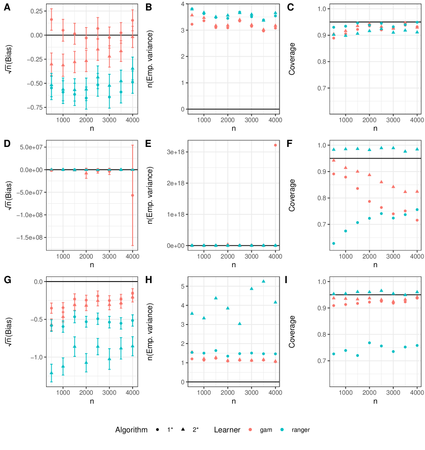
Figure 1: Sample size against Bias (1st column), variance (2nd) and 95% Wald CI coverage (3rd) for $\hat{\Psi}$ (plots A,B,C), $\hat{\psi}$ using the direct approach (plots D,E,F), and $\hat{\psi}$ using the quasi-oracle approach (plots G,H,I). We highlight that the y-axis limits change between row of the bias and variance plots. The black horizontal line represents 0 bias and variance, and 95% coverage respectively.

8 Warfarin dose example

We illustrate the proposed estimators using the IWPC (International Warfarin Pharmacogenetics Consortium,, 2009) dataset, which has also been reanalysed several times in literature on dynamic treatment rule estimation (Schulz and Moodie,, 2021; Wallace et al.,, 2018; Chen et al.,, 2016). Reproduction code for this analysis is available at github.com/ohines/alse. The data consists of $n=1732$ patients receiving Warfarin therapy, which is a commonly prescribed anticoagulant used to treat thrombosis and thromboembolism. We consider least squares estimands for the effect of Warfarin dose $(A)$ on international normalised ratio (INR) $(Y)$, which is a measure of blood clotting function, given 13 other patient characteristics $(\bm{Z})$, including genetic data, as described in International Warfarin Pharmacogenetics Consortium, (2009).

Fitted models were obtained using the Super Learner (van der Laan et al.,, 2007), an ensemble learning method, implemented in the SuperLearner package in R. This used 20 cross validation folds, and a ‘learner library’ containing various routines (glm, glmnet, gam, xgboost, ranger). Additional results which use the ‘discrete’ Super Learner for model fitting are presented in Appendix D. The discrete Super Learner selects the regression algorithm in the learner library which minimises a cross validated estimate of e.g. the mean squared error loss, whereas the Super Learner minmizes the same loss by taking a convex combination of learners. For the sample splitting algorithms (Algorithm 2), $K=20$ folds were chosen (between 10 to 20 folds is typical for cross-fitting procedures).

The results, presented in Table 1, suggest that increased Warfarin is associated with an increase in INR. We see that the estimators for $\Psi$ tend to have narrower confidence intervals than estimators for $\psi$, with commensurately smaller Wald based P-values for the corresponding ‘zero-effect’ null (i.e. the null hypothesis that $\Psi=0$ vs. the null hypothesis that $\psi=0$). This type of difference is to be expected, based on the efficiency arguments presented in Section 5. Additionally, the estimators for $\psi$, which use the R-learner for conditional effect estimation (Algorithms 1B and 2B) give more credible estimates than those that use the direct approach (Algorithms 1A and 2A), in the sense that they are of a similar order of magnitude to the $\Psi$ estimates. Moreover, we see that sample splitting leads to more credible estimates, compared with no sample splitting, as evident in Algorithms 2A versus 1A. This difference is because sample splitting helps to control for overfitting of the functional estimators.

Table 1: Least squares estimands applied to IWPC data. Values indicate point estimates, given in INR/(mg/week), with 95% Wald confidence intervals given in parentheses. P-values represent those obtained from a Wald based test of the null hypothesis that the estimand is 0.

Estimand	Algorithm	Result
$\Psi$	1	2.01$\times 10^{-3}$ (0.731$\times 10^{-3}$,3.28$\times 10^{-3}$) p=0.002
$\Psi$	2	1.91$\times 10^{-3}$ (0.70$\times 10^{-3}$,3.12$\times 10^{-3}$) p=0.002
$\psi$	1A	-6.39 (-19.4,6.65) p=0.33
$\psi$	2A	0.611 (-0.664,1.89) p=0.35
$\psi$	1B	1.59$\times 10^{-3}$ (-0.0660$\times 10^{-3}$,3.25$\times 10^{-3}$) p=0.06
$\psi$	2B	1.55$\times 10^{-3}$ (-0.329$\times 10^{-3}$,3.42$\times 10^{-3}$) p=0.11

9 Extensions

We showed that least squares estimands are weighted ADEs with non-negative exposure weights, using Theorem 1 and Lemma 1.1. Here we apply these results again to propose other weighted ADEs that reduce to the ADE (Example 1) when $A$ follows one of a three standard parametric distributions given $\bm{Z}$.

We consider the form of (10) when the distribution of $A$ given $\bm{Z}=\bm{z}$ follows a normal, gamma $(A>0)$ or asymmetric Laplace distribution (Yu and Zhang,, 2005) with the respective density functions

$$f_{1}(a|\mu,\sigma) =\frac{1}{\sqrt{2\pi}\sigma}\exp\left\{-\frac{(a-\mu)^{2}}{2\sigma^{2}}\right\}$$

$$f_{2}(a|\alpha,\beta) =\frac{\beta}{\Gamma(\alpha)}a^{\alpha-1}\exp(-\beta a)$$

$$f_{3}(a|p,\sigma,x_{0}) =\frac{p(1-p)}{\sigma}\exp\left\{-(a-a_{0})\frac{\Theta(a-a_{0})-p}{\sigma}\right\}$$

where $a_{0}$ is a known value and the parameters $\mu,\sigma>0,\alpha>0,\beta>0,p\in(0,1)$ are all constant given $\bm{Z}=\bm{z}$. Also, $\Gamma(.)$ represents the gamma function and $\Theta(u)$ is a step function which takes the value 1 when $u>0$ and $0$ otherwise. Plugging these density functions, in turn, into (10) gives

$$-\frac{d\log f_{1}(a|\mu,\sigma^{2})}{da} =\frac{a-\mu}{\sigma^{2}}$$

$$-\frac{d\log f_{2}(a|\alpha,\beta)}{da} =(1-\alpha)a^{-1}+\beta$$

$$-\frac{d\log f_{3}(a|p,\sigma,x_{0})}{da} =\frac{\Theta(a-a_{0})-p}{\sigma}.$$

Technically the third equation above describes the derivative for $a\neq a_{0}$, since $f_{3}(a|p,\sigma,a_{0})$ is not differentiable at this point. This is not problematic, however, since these expressions are used only to inspire well defined contrast functions. It is readily seen that all three are of the form of a known function of $a$ up to centring and scaling by parameters which are constant given $\bm{z}$. In particular, they are of the form in (8) where $v(a,\bm{z})$ is replaced with the known functions, $a,a^{-1}$ and $\Theta(a-a_{0})$ respectively. According to (9), therefore, these choices imply the weighted ADEs,

$$\theta_{w,1} =E\left\{w(\bm{Z})\frac{\mathrm{cov}(A,Y|\bm{Z})}{\mathrm{var}(A|\bm{Z})}\right\}$$

$$\theta_{w,2} =E\left\{w(\bm{Z})\frac{\mathrm{cov}(A^{-1},Y|\bm{Z})}{\mathrm{cov}(A^{-1},A|\bm{Z})}\right\}$$

$$\theta_{w,3} =E\left\{w(\bm{Z})\frac{E(Y|A>a_{0},\bm{Z})-E(Y|A\leq a_{0},\bm{Z})}{E(A|A>a_{0},\bm{Z})-E(A|A\leq a_{0},\bm{Z})}\right\}$$

which, for $w(\bm{Z})=1$, reduce to the ADE when $A$ respectively follows the normal, gamma, and asymmetric Laplace distribution conditional on $\bm{Z}$. The estimand $\theta_{w,1}$ is the least squares estimand studied in this paper, and is thus further motivated by its connection to normally distributed exposures. These estimands, however, are nonparametrically well defined, even when the exposure does not follow the associated parametric distribution or indeed when it is not continuous or $\mu^{\prime}(a,\bm{z})$ does not exist. This raises the questions of the extent to which $\theta_{w,2}$ and $\theta_{w,3}$ are useful and interpretable estimands in their own right, in what contexts one might use them, how $w(\bm{Z})$ should be chosen, and how best they should be estimated. Such questions are beyond the scope of the current work. We remark that $\theta_{w,3}$ with the (unnormalised) weight $w(\bm{Z})=E(A|A>a_{0},\bm{Z})-E(A|A\leq a_{0},\bm{Z})$ reduces to

$$E\left\{E(Y|A>a_{0},\bm{Z})-E(Y|A\leq a_{0},\bm{Z})\right\},$$

which identifies the ATE of a dichotomised exposure on outcome when $\bm{Z}$ is sufficient to adjust for confounding between exposure and outcome.

10 Discussion

The current work makes several contributions to the literature on weighted ADEs for a single covariate (exposure). In particular we derive sufficiency conditions on a pair of functions $(w,l)$, such that the product $w(\bm{z})l(a|\bm{z})$ is the Riesz representer of a weighted ADE.

We next show that least squares estimands, which are estimands connected to partially linear model projections, are in fact weighted ADEs for a particular choice of weight function. We further motivate least squares estimands by considering the Riesz representer that minimises the nonparametric efficiency bound of the weighted ADE, when the representer is known and the outcome is homoscedastic. Our efficiency analysis extends the methods of Crump et al., (2006) to the setting of a continuous exposures.

We further use the influence curves of the proposed least squares estimands to derive efficient one-step estimators, $\hat{\Psi}$ and $\hat{\psi}$, the latter of which generalises the AIPW to the setting of a continuous exposure. To estimate the working models we recommend a quasi-oracle approach based on the R-learner (Nie and Wager,, 2021). Our proposal involves a novel quasi-oracle learner for the inverse variance, $1/\mathrm{var}(A|\bm{Z})$, which is designed to mitigate extreme weighting in the estimator.

Our recommendation is that the least squares estimands $\psi$ and $\Psi$ be inferred for the exploratory analysis of the main effect of an exposure on an outcome. The resulting quantities may be interpreted as weighted ADEs with data-adaptive exposure weights $w(a|\bm{z})$. These weights happen to equal $1$ when the exposure is conditionally normally distributed. Additionally, a causal interpretation related to infinitesimal shift interventions may be ascribed to weighted ADEs (and hence least squares estimands), as described by Rothenhäusler and Yu, (2019).

Appendix A Supplementary Materials

Derivation of (4)

Assume (C1), $\tilde{f}(a|\bm{z})\equiv w(a|\bm{z})f(a|\bm{z})$ is differentiable, and (C2), $\tilde{f}(s|\bm{z})=\tilde{f}(t|\bm{z})=0$, where $s$ and $t$ denote the boundary of the support of $A$. Integration by parts gives

$$E\{w(A|\bm{Z})\mu^{\prime}(A,\bm{Z})|\bm{Z}=\bm{z}\} =\int_{s}^{t}\mu^{\prime}(a,\bm{z})\tilde{f}(a|\bm{z})da$$

$$=\mu(t,\bm{z})\tilde{f}(t|\bm{z})-\mu(s,\bm{z})\tilde{f}(s|\bm{z})-\int_{s}^{t}\mu(a,\bm{z})\tilde{f}^{\prime}(a|\bm{z})da$$

$$=E\{l(A|\bm{Z})\mu(A,\bm{Z})|\bm{Z}=\bm{z}\}$$

where we let $l(a|\bm{z})=-\tilde{f}^{\prime}(a|\bm{z})/f(a|\bm{z})$, as in (4). To motivate Theorem 1, note that inverting (4) gives

$$\tilde{f}(a|\bm{z}) =-\int_{s}^{a}l(a^{*}|\bm{z})f(a^{*}|\bm{z})da^{*}=-E\{l(A|\bm{Z})|A\leq a,\bm{Z}=\bm{z}\}F(a|\bm{z})$$

Proof of Theorem 1

Theorem 1 essentially follows by the integration by parts argument above. Rather than work with the exposure weight in (5) directly, we consider the function $\tilde{f}(a|\bm{z})\equiv w(a|\bm{z})f(a|\bm{z})$. Our goal is to show that this integrates to 1, i.e. $E\{w(A|\bm{Z})|\bm{Z}\}=1$, and that it satisfies (C2). Note (C1) is satisfied since $\tilde{f}^{\prime}(a|\bm{z})=-l(a|\bm{z})f(a|\bm{z})$ by the fundamental theorem of calculus. To do so, let $\Theta(u)$ denote a step function which is 1 for $u\geq 0$ and 0 for $u<0$ and hence,

$$\tilde{f}(a|\bm{z}) =-\int_{s}^{t}\Theta(a-a^{*})l(a^{*}|\bm{z})dP(a^{*}|\bm{z})$$

where $dP(a|\bm{z})$, is the probability measure of $A$ given $\bm{Z}$. Integrating over $a$, gives

$$\int_{s}^{t}\tilde{f}(a|\bm{z})da =\int_{s}^{t}\left[\int_{s}^{t}-\Theta(a-a^{*})da\right]l(a^{*}|\bm{z})dP(a^{*}|\bm{z})$$

For the part in the square brackets,

$$\int_{s}^{t}-\Theta(a-a^{*})da=\int_{a^{*}}^{t}-1dx=a^{*}-t$$

Hence,

$$\int_{s}^{t}\tilde{f}(a|\bm{z})da =E\{l(A|\bm{Z})A|\bm{Z}=\bm{z}\}-tE\{l(A|\bm{Z})|\bm{Z}=\bm{z}\}=1$$

Thus $\tilde{f}(a|\bm{z})$ integrates to $1$. We remark that when the exposure weight is non-negative then $\tilde{f}(a|\bm{z})$ is a density function. Next we show $\tilde{f}(a|\bm{z})$ satisfies (C2) when $A$ is a continuous random variable. Since $a^{*}\leq t$, then $\Theta(t-a^{*})=1$, hence

$$\tilde{f}(t|\bm{z}) =-\int_{s}^{t}l(a^{*}|\bm{z})dP(a^{*}|\bm{z})=-E\{l(A|\bm{Z})|\bm{Z}=\bm{z}\}=0$$

Similarly, since $a^{*}\geq s$, then $\Theta(s-a^{*})=1$ only for $a^{*}=s$,

$$\tilde{f}(s|\bm{z}) =-\int_{s}^{s}l(a^{*}|\bm{z})dP(a^{*}|\bm{z})=-l(s|\bm{z})P(A=s|\bm{Z}=\bm{z})$$

Since $A$ is continuous, $P(A=s|\bm{Z}=\bm{z})=0$. This completes the proof.

Proof of Lemma 1.1

First we prove that Theorem 1 is satisfied when $l(a|\bm{z})$ is monotonically increasing and (D1) $E\{l(A|\bm{Z})|\bm{Z}\}=0$ and (D2) $E\{l(A|\bm{Z})A|\bm{Z}\}=1$ almost surely. We split $l(a|\bm{z})$ into a positive and negative part by defining two non-negative functions, $l^{+}(a|\bm{z})=\max\{l(a|\bm{z}),0\}$ and $l^{-}(a|\bm{z})=\max\{-l(a|\bm{z}),0\}$ such that, $l(a|\bm{z})=l^{+}(a|\bm{z})-l^{-}(a|\bm{z})$. It follows from (D1) that,

$$E\{l^{+}(A|\bm{Z})|\bm{Z}\} =E\{l^{-}(A|\bm{Z})|\bm{Z}\}.$$

This equality is satisfied by $l^{+}(a|\bm{z})=l^{-}(a|\bm{z})=0$, however this solution violates (D2), hence the positive and negative parts are both non-zero. Since, $l(a|\bm{z})$ is monotonically increasing there must be some value, $c=c(\bm{z})$, on the support of $A$, such that the positive part is zero for $a<c$ and the negative part is zero for $a\geq c$, i.e.

$$l(a|\bm{z}) =l^{+}(a|\bm{z})\Theta(a-c)-l^{-}(a|\bm{z})\{1-\Theta(a-c)\}.$$

First consider the inequality in (5) when $a<c$,

$$\int_{s}^{a}l(a^{*}|\bm{z})dP(a^{*}|\bm{z}) =-\int_{s}^{a}l^{-}(a^{*}|\bm{z})dP(a^{*}|\bm{z})\leq 0.$$

When $a\geq c$,

$$\int_{s}^{a}l(a^{*}|\bm{z})dP(a^{*}|\bm{z}) =\int_{c}^{a}l^{+}(a^{*}|\bm{z})dP(a^{*}|\bm{z})-\int_{s}^{c}l^{-}(a^{*}|\bm{z})dP(a^{*}|\bm{z}).$$

The first part on the right hand side is $\leq E\{l^{+}(A|\bm{Z})|\bm{Z}=\bm{z}\}$ and the second part is $=E\{l^{-}(A|\bm{Z})|\bm{Z}=\bm{z}\}$ therefore, in both cases,

$$\int_{s}^{a}l(a^{*}|\bm{z})dP(a^{*}|\bm{z}) \leq 0$$

Hence $\tilde{f}(a|\bm{z})\geq 0$, so the inequality in (5) is satisfied. The proof is completed by verifying that the contrast function in (8) is monotonically increasing when $v(a,\bm{z})$ is monotonically increasing or decreasing but not constant. This is fairly straight forward and we note that the decreasing case follows from the increasing case since (8) is invariant to replacing $v(a,\bm{z})$ with $-v(a,\bm{z})$.

Proof of Theorem 2

An efficient estimator of $\theta_{w}$ is regular asymptotically linear, such that

$$\hat{\theta}_{w}=\theta_{w}+n^{-1}\sum_{i=1}^{n}\phi_{\theta,w}(\bm{o}_{i})+o_{p}(n^{-1/2})$$

where $\phi_{\theta,w}(\bm{o})$ is the influence curve of $\theta_{w}$ in (12). Hence,

$$n^{1/2}(\hat{\theta}_{w}-\theta_{w,S})=n^{-1/2}\sum_{i=1}^{n}w(\bm{z}_{i})l(a_{i}|\bm{z}_{i})\{y_{i}-\mu(a_{i},\bm{z}_{i})\}+o_{p}(1)$$

By the central limit theorem, $n^{1/2}(\hat{\theta}_{w}-\theta_{w,S})\overset{d}{\to}\mathcal{N}\left(0,V\right)$, where the efficiency bound is

$$V =E\left\{w(\bm{Z})^{2}l(A|\bm{Z})^{2}\{Y-\mu(A,\bm{Z})\}^{2}\right\}$$

$$=E\left\{w(\bm{Z})^{2}l(A|\bm{Z})^{2}E\left(\{Y-\mu(A,\bm{Z})\}^{2}|X,\bm{Z}\right)\right\}$$

$$=E\left\{w(\bm{Z})^{2}l(A|\bm{Z})^{2}\sigma^{2}(A,\bm{Z})\right\}$$

$$=E\left\{w(\bm{Z})^{2}E[l(A|\bm{Z})^{2}\sigma^{2}(A,\bm{Z})|\bm{Z}]\right\}$$

Minimizing $E\{l^{2}(A|\bm{Z})\sigma^{2}(A,\bm{Z})|\bm{Z}=\bm{z}\}$ subject to $E\{l(A|\bm{Z})|\bm{Z}=\bm{z}\}=0$ and $E\{l(A|\bm{Z})A|\bm{Z}=\bm{z}\}=1$. Using Lagrange multipliers, $\lambda_{1}$, $\lambda_{2}$, which are both constant given $\bm{Z}=\bm{z}$,

$$\int l^{2}(a|\bm{z})\sigma^{2}(a,\bm{z})-2\lambda_{1}l(a|\bm{z})-2\lambda_{2}\{l(a|\bm{z})a-1\}dP(a|\bm{z})$$

Differentiating the Lagrangian with respect to $l(a|\bm{z})$ and setting equal to zero gives.

$$l(a|\bm{z})=\frac{\lambda_{1}+\lambda_{2}a}{\sigma^{2}(a,\bm{z})}$$

Applying the two constraints fixes $\lambda_{1}$ and $\lambda_{2}$, giving the contrast function stated in the main theorem. Next we consider optimizing for $w(\bm{z})$ under the constraint $E\{w(\bm{Z})\}=1$. Again, the use of Lagrange multipliers gives

$$\int w(\bm{z})^{2}E\{l^{2}(A|\bm{Z})\sigma^{2}(A,\bm{Z})|\bm{Z}=\bm{z}\}-2\lambda_{3}\{w(\bm{z})-1\}dP(\bm{z})$$

and differentiating the Lagrangian with respect to $w(\bm{z})$ and setting equal to zero gives

$$w(\bm{z})=\frac{\lambda_{3}}{E\{l^{2}(A|\bm{Z})\sigma^{2}(A,\bm{Z})|\bm{Z}=\bm{z}\}}$$

The constant, $\lambda_{3}$ is fixed by the constraint, completing the proof.

Proof of Lemma 4.1

Let $\alpha(w)$ be a function such that $\alpha(w)=0$ for $w=0$ and $\alpha(w)=1/w$ otherwise. Consider the expectation

$$E\left[W\left\{V\alpha(W)-g(\bm{Z})\right\}^{2}\right] =E\left\{V^{2}\alpha^{2}(W)W\right\}+E\left\{g^{2}(\bm{Z})W-2g(\bm{Z})VW\alpha(W)\right\}$$

$$=E\left\{V^{2}\alpha^{2}(W)W\right\}+E\left\{g^{2}(\bm{Z})E(W|\bm{Z})-2g(\bm{Z})E\{VW\alpha(W)|\bm{Z}\}\right\}$$

For the purposes of minimization over $g(.)$ the first term on the right hand side can be discarded since it does not depend on $g(.)$. Hence

$$\operatorname*{arg\,min}_{g\in\mathcal{F}}E\left[W\left\{V\alpha(W)-g(\bm{Z})\right\}^{2}\right] =\operatorname*{arg\,min}_{g\in\mathcal{F}}E\left\{g^{2}(\bm{Z})E(W|\bm{Z})-2g(\bm{Z})E\{VW\alpha(W)|\bm{Z}\}\right\}$$

By the calculus of variations, the minimiser $g^{*}(\bm{z})$ satisfies,

$$g^{*}(\bm{z})E(W|\bm{Z}=\bm{z})=E\{VW\alpha(W)|\bm{Z}=\bm{z}\}$$

Since $W\neq 0$ almost surely,

$$E\{VW\alpha(W)|\bm{Z}\} =E\{VW\alpha(W)|W\neq 0,\bm{Z}\}$$

$$=E(V|W\neq 0,\bm{Z})$$

$$=E(V|\bm{Z}).$$

Hence the result follows provided that $E(W|\bm{Z})\neq 0$ which is true since $W>0$ almost surely.

Appendix B Exposure weight for the least squares estimand

Here we examine the exposure weight $w(a|\bm{z})$ in (11), which is associated with the least squares estimands, $\psi$ and $\Psi$ in the main text. We remark that the this weight depends on the unknown distribution $P_{0}$ through the distribution of $A$ given $Z$, like the density weight in Example 2 of the main text. The exposure weight for least squares estimands is therefore data-adaptive, though it is not necessary to compute this weight to estimate $\psi$ or $\Psi$.

We consider the form of this exposure weight under various parametric distributions $f(a|\bm{z})$ in Pearson’s distribution family. Table 2 summarises the functional form of the “unnormalised” exposure weight, with details provided in Examples 3 to 9 below. We say that the unnormalised exposure weight is the exposure weight $w(a|\bm{z})$ up to multiplicative factors which are constant given $\bm{z}$, i.e. which ensure that $E\{w(A|\bm{Z})|\bm{Z}\}=1$. In particular, for each distribution in Table 2, the “normalised” weight is obtained as $w(a|\bm{z})=\tilde{w}(a|\bm{z})/E\{\tilde{w}(A|\bm{Z})|\bm{Z}=\bm{z}\}$.

Table 2: “Unnormalised” exposure weight $\tilde{w}(a|\bm{z})$ for least squares estimands when the distribution of $A$ given $Z$ follows a parametric distribution. Proofs below.

Exposure Distribution	Support	$\tilde{w}(a|z)$
Normal	$A\in(-\infty,\infty)$	$1$
Gamma	$A>0$	$a$
Inverse-Gamma	$A>0$	$a^{2}$
Beta	$A\in(0,1)$	$a(1-a)$
Beta Prime	$A>0$	$a(1+a)$
t-distribution (d.o.f. $=\nu(\bm{z})$)	$A\in(-\infty,\infty)$	$1+\frac{a^{2}}{\nu(\bm{z})}$

When deriving the results in Table 2, it is helpful to consider the function $\tilde{f}(a|\bm{z})\equiv w(a|\bm{z})f(a|\bm{z})$. Since the exposure weight is non-negative (by Lemma 1.1), and $E\{w(A|\bm{Z})|\bm{Z}\}=1$, it follows that $\tilde{f}(a|\bm{z})$ is a density function. Letting $s$ denote the lower boundary of the support of $A$ then we write this density function as

$$\tilde{f}(a|\bm{z})=\int_{s}^{a}\frac{\mu(\bm{z})-a^{*}}{\beta(\bm{z})}f(a^{*}|\bm{z})da$$

We use this function as a tool to derive the exposure weight in the following examples. Each example requires verifying a derivative result, which follows from standard calculus and the Gamma function property $\nu\Gamma(\nu)=\Gamma(\nu+1)$.

Example 4 (Normal distribution).

Letting $f(a|\mu,\beta)$ denote the normal distribution, with mean $\mu=\mu(\bm{z})$ and variance $\beta=\beta(\bm{z})$, we claim that $\tilde{f}(a|\mu,\beta)=f(a|\mu,\beta)$, which implies an exposure weight $w(a|\bm{z})=\tilde{f}(a|\mu,\beta)/f(a|\mu,\beta)=1$. To verify this claim, note that

$$\frac{d}{da}f(a|\mu,\beta)=\frac{\mu-a}{\beta}f(a|\mu,\beta).$$

Hence,

$$\tilde{f}(a|\bm{z})=\int_{-\infty}^{a}\left\{\frac{d}{da^{*}}f(a^{*}|\mu,\beta)\right\}da^{*}$$

and the result follows by the fundamental theorem of calculus. The unitary weight of the normal distribution implies that the least squares estimand $\psi$ recovers the average derivative effect when the exposure $A$ is normally distributed given $Z$.

Example 5 (Gamma distribution).

The Gamma distribution, with shape parameter, $\nu=\nu(\bm{z})>0$, and rate parameter $\tau=\tau(\bm{z})>0$, has the density

$$f(a|\nu,\tau)=\frac{\tau^{\nu}}{\Gamma(\nu)}a^{\nu-1}\exp(-\tau a)$$

for $a>0$ and 0 otherwise.

We claim that, for the gamma distribution, $\tilde{f}(a|\nu,\tau)=f(a|\nu+1,\tau)$. As in Example 3, it is sufficient to verify that

$$\frac{d}{da}f(a|\nu+1,\tau)=\frac{\mu-a}{\beta}f(a|\nu,\tau)$$

where the mean and variance are $\mu=\nu/\tau$ and $\beta=\nu/\tau^{2}$. Therefore, the exposure weight is

$$w(a|\bm{z})=\frac{f(a|\nu+1,\tau)}{f(a|\nu,\tau)}=\frac{a}{\mu}.$$

This linear weight assigns unitary weight to the mean value $a=\mu$, with larger weight given to values above the mean.

Example 6 (Inverse Gamma distribution).

The Inverse Gamma distribution, with shape parameter, $\nu=\nu(\bm{z})>0$, and scale parameter $\tau=\tau(\bm{z})>0$, has the density

$$f(a|\nu,\tau)=\frac{\tau^{\nu}}{\Gamma(\nu)}a^{-\nu-1}\exp(-\tau/a)$$

for $a>0$ and 0 otherwise. We claim that, for the inverse-gamma distribution, $\tilde{f}(a|\nu,\tau)=f(a|\nu-2,\tau)$. As before, it is sufficient to verify that

$$\frac{d}{da}f(a|\nu-2,\tau)=\frac{\mu-a}{\beta}f(a|\nu,\tau)$$

where the mean and variance are $\mu=\tau/(\nu-1)$ and

$$\beta=\frac{\tau^{2}}{(\nu-1)^{2}(\nu-2)}.$$

Therefore, the exposure weight is

$$w(a|\bm{z})=\frac{f(a|\nu-2,\tau)}{f(a|\nu,\tau)}=\frac{a^{2}}{\beta+\mu^{2}}.$$

Example 7 (Beta distribution).

The beta distribution, with shape parameters, $\nu=\nu(\bm{z})>0$, and $\tau=\tau(\bm{z})>0$, has the density

$$f(a|\nu,\tau)=\frac{\Gamma(\nu+\tau)}{\Gamma(\nu)\Gamma(\tau)}a^{\nu-1}(1-a)^{\tau-1}$$

for $a\in[0,1]$ and 0 otherwise. We claim that, for the beta distribution, $\tilde{f}(a|\nu,\tau)=f(a|\nu+1,\tau+1)$. As before, it is sufficient to verify that

$$\frac{d}{da}f(a|\nu+1,\tau+1)=\frac{\mu-a}{\beta}f(a|\nu,\tau)$$

where the mean and variance are $\mu=\nu/(\nu+\tau)$ and

$$\beta=\frac{\nu\tau}{(\nu+\tau)^{2}(\nu+\tau+1)}.$$

Therefore, the exposure weight is

$$w(a|\bm{z})=\frac{f(a|\nu+1,\tau+1)}{f(a|\nu,\tau)}=\frac{a(1-a)}{\mu(1-\mu)-\beta}.$$

This quadratic weight is at a maximum when $a=1/2$, with very little weight assigned to values close to $a=0,1$.

Example 8 (Beta-prime distribution).

The beta-prime distribution, with shape parameters, $\nu=\nu(\bm{z})>2$, and $\tau=\tau(\bm{z})>0$, has the density

$$f(a|\nu,\tau)=\frac{\Gamma(\nu+\tau)}{\Gamma(\nu)\Gamma(\tau)}a^{\nu-1}(1+a)^{-\nu-\tau}$$

for $a\geq 0$. We claim that, for the beta-prime distribution, $\tilde{f}(a|\nu,\tau)=f(a|\nu+1,\tau-2)$. As before, it is sufficient to verify that

$$\frac{d}{da}f(a|\nu+1,\tau-2)=\frac{\mu-a}{\beta}f(a|\nu,\tau)$$

where the mean and variance are $\mu=\nu/(\tau-1)$ and

$$\beta=\frac{\nu(\nu+\tau-1)}{(\tau-2)(\tau-1)^{2}}.$$

Therefore, the exposure weight is

$$w(a|\bm{z})=\frac{f(a|\nu+1,\tau-2)}{f(a|\nu,\tau)}=\frac{a(1+a)}{\mu(1+\mu)+\beta}.$$

Example 9 (Student’s t-distribution).

The t-distribution, with $\nu=\nu(\bm{z})>2$ degrees of freedom, location parameter $\mu=\mu(\bm{z})$, and scale parameter $\tau=\tau(\bm{z})$ has the density

$$f(a|\nu,\mu,\tau^{2})=\frac{\Gamma\left(\frac{\nu+1}{2}\right)}{\sqrt{\nu\pi}\tau\Gamma\left(\frac{\nu}{2}\right)}\left(1+\frac{(a-\mu)^{2}}{\nu\tau^{2}}\right)^{-\frac{\nu+1}{2}}$$

We claim that, for the t-distribution,

$$\tilde{f}(a|\nu,\mu,\tau^{2})=f(a|\nu-2,\mu,\beta)$$

where $\beta=\tau^{2}\nu/(\nu-2)$ is the variance of the t-distribution. As before, it is sufficient to verify that

$$\frac{d}{da}f(a|\nu-2,\mu,\beta)=\frac{\mu-a}{\beta}f(a|\nu,\mu,\tau^{2}).$$

Therefore, the exposure weight is

$$w(a|\bm{z})=\frac{f(a|\nu-2,\mu,\beta)}{f(a|\nu,\mu,\tau^{2})}=\frac{\left(1+\frac{(a-\mu)^{2}}{\nu\tau^{2}}\right)}{\left(1+\frac{1}{\nu-2}\right)}.$$

As $\nu\to\infty$ then $w(a|\bm{z})\to 1$. This is expected since the the t-distribution tends to a normal distribution, with mean $\mu$, and variance $\tau^{2}$ in this limit. Note that in Table 2, this weight is reported for $\mu=0,\tau=1$.

Appendix C Estimator Asymptotic Distribution

In this Appendix we use a common empirical processes notation, where we define linear operators $P$ and $\mathbb{P}_{n}$ such that for some function $h(\bm{O})$, $P\{h(\bm{O})\}\equiv E\{h(\bm{O})\}$ and $\mathbb{P}_{n}\{h(\bm{O})\}\equiv n^{-1}\sum_{i=1}^{n}h(\bm{o}_{i})$.

C.1 Proof of Theorem 3

Define

$$\hat{\phi}_{\psi}(\bm{o}) =\frac{\{y-\hat{\mu}(\bm{z})\}\{a-\hat{\pi}(\bm{z})\}-\hat{\lambda}(\bm{z})\{a-\hat{\pi}(\bm{z})\}^{2}}{\hat{\beta}(\bm{z})}+\hat{\lambda}(\bm{z})-\hat{\psi}_{0}$$

where $\hat{\psi}_{0}=\mathbb{P}_{n}\{\hat{\lambda}(\bm{Z})\}$ denotes an initial estimate of $\psi$. Without making any restrictions we write

$$\hat{\psi}-\psi =(\mathbb{P}_{n}-P)\{\phi_{\psi}(\bm{O})\}+R_{n}+H_{n}$$ (16)

$$\hat{\psi} \equiv\hat{\psi}_{0}+\mathbb{P}_{n}\{\hat{\phi}_{\psi}(\bm{O})\}$$ (17)

$$R_{n} \equiv\hat{\psi}_{0}-\psi+P\{\hat{\phi}_{\psi}(\bm{O})\}$$ (18)

$$H_{n} \equiv(\mathbb{P}_{n}-P)\{\hat{\phi}_{\psi}(\bm{O})-\phi_{\psi}(\bm{O})\}.$$ (19)

We will show that the remainder therm $R_{n}=o_{P}(n^{-1/2})$ and the empirical process term $H_{n}=o_{P}(n^{-1/2})$, and hence the result follows since $P\{\phi_{\psi}(\bm{O})\}=0$.

The remainder term

To simplify notation, we will omit function arguments, e.g. $\mu=\mu(\bm{Z})$ with similar for $\hat{\mu},\lambda,\hat{\lambda},\pi,\hat{\pi},\hat{\beta},\beta$. Since $\psi=E[\lambda]$ we can write the remainder term as

$$R_{n} =E\left[\frac{(Y-\hat{\mu})(A-\hat{\pi})-\hat{\lambda}(A-\hat{\pi})^{2}}{\hat{\beta}}+\hat{\lambda}-\lambda\right]$$

Note that

$$E[(Y-\hat{\mu})(A-\hat{\pi})|\bm{Z}] =\lambda\beta+(\mu-\hat{\mu})(\pi-\hat{\pi})$$

$$E[(A-\hat{\pi})^{2}|\bm{Z}] =\beta+(\pi-\hat{\pi})^{2}$$

and hence

$$R_{n} =E\left[\frac{(\pi-\hat{\pi})\{\mu-\hat{\mu}-\hat{\lambda}(\pi-\hat{\pi})\}+(\lambda-\hat{\lambda})(\beta-\hat{\beta})}{\hat{\beta}}\right]$$

Using the inequality, $(a+b)^{2}\leq 2(a^{2}+b^{2})$,

$$\frac{R_{n}^{2}}{2} \leq\underbrace{E\left[\frac{(\pi-\hat{\pi})\{\mu-\hat{\mu}-\hat{\lambda}(\pi-\hat{\pi})\}}{\hat{\beta}}\right]^{2}}_{\text{first remainder}}+\underbrace{E\left[\frac{(\lambda-\hat{\lambda})(\beta-\hat{\beta})}{\hat{\beta}}\right]^{2}}_{\text{second remainder}}$$ (20)

We will show that the two remainder terms on the right hand side are $o_{p}(n^{-1})$. For the first remainder, the Cauchy-Schwarz inequality gives

$$E\left[\frac{(\pi-\hat{\pi})\{\mu-\hat{\mu}-\hat{\lambda}(\pi-\hat{\pi})\}}{\hat{\beta}}\right]^{2} \leq E\left[\frac{(\pi-\hat{\pi})^{2}}{\hat{\beta}}\right]E\left[\frac{\{\mu-\hat{\mu}-\hat{\lambda}(\pi-\hat{\pi})\}^{2}}{\hat{\beta}}\right]$$

$$\leq\left(\frac{1}{\epsilon^{2}}\right)E\left[(\pi-\hat{\pi})^{2}\right]E\left[\{\mu-\hat{\mu}-\hat{\lambda}(\pi-\hat{\pi})\}^{2}\right]$$

$$\leq\left(\frac{2}{\epsilon^{2}}\right)E\left[(\pi-\hat{\pi})^{2}\right]\left\{E\left[(\mu-\hat{\mu})^{2}\right]+E\left[\hat{\lambda}^{2}(\pi-\hat{\pi})^{2}\right]\right\}$$

$$\leq\left(\frac{2}{\epsilon^{2}}\right)E\left[(\pi-\hat{\pi})^{2}\right]\left\{E\left[(\mu-\hat{\mu})^{2}\right]+K^{2}E\left[(\pi-\hat{\pi})^{2}\right]\right\}$$

To obtain the second inequality above, we choose $\epsilon>0$ such that $\hat{\beta}\geq\epsilon$ almost surely, and to obtain the third inequality we once again apply the inequality $(a+b)^{2}\leq 2(a^{2}+b^{2})$. It therefore follows from (A1) that the first remainder in (20) is $o_{p}(n^{-1})$.

For the second remainder in (20), the Cauchy-Schwarz inequality gives

$$E\left[\frac{(\lambda-\hat{\lambda})(\beta-\hat{\beta})}{\hat{\beta}}\right]^{2} \leq E\left[\frac{(\lambda-\hat{\lambda})^{2}}{\hat{\beta}}\right]E\left[\frac{(\beta-\hat{\beta})^{2}}{\hat{\beta}}\right]$$

$$\leq\left(\frac{1}{\epsilon^{2}}\right)E\left[(\lambda-\hat{\lambda})^{2}\right]E\left[(\beta-\hat{\beta})^{2}\right]$$

which is $o_{P}(n^{-1})$ under (A2). Hence $R_{n}=o_{P}(n^{-1/2})$.

The empirical process term

First write the empirical process term as the sum of four terms

$$H_{n} =(\mathbb{P}_{n}-P)\{\psi-\hat{\psi}_{0}\}$$

$$+(\mathbb{P}_{n}-P)\{\hat{\lambda}-\lambda\}$$

$$+(\mathbb{P}_{n}-P)\left\{\frac{\hat{u}(\bm{O})}{\hat{\beta}}-\frac{u(\bm{O})}{\beta}\right\}$$

$$+(\mathbb{P}_{n}-P)\left\{\frac{\hat{\lambda}\hat{v}(\bm{O})}{\hat{\beta}}-\frac{\lambda v(\bm{O})}{\beta}\right\}$$

where

$$\hat{u}(\bm{O}) \equiv(Y-\hat{\mu})(A-\hat{\pi})$$

$$u(\bm{O}) \equiv(Y-\mu)(A-\pi)$$

$$\hat{v}(\bm{O}) \equiv(A-\hat{\pi})^{2}$$

$$v(\bm{O}) \equiv(A-\pi)^{2}$$

Note that the first term is zero since $(\mathbb{P}_{n}-P)\{\psi-\hat{\psi}_{0}\}=(\psi-\hat{\psi}_{0})(\mathbb{P}_{n}-P)\{1\}=0$. When the Donsker condition holds, then, by Lemma 19.24 of van der Vaart, (2013), the second term is $o_{P}(n^{-1/2})$ provided (i) that $E\{(\hat{\lambda}-\lambda)^{2}\}=o_{p}(1)$, the third term is $o_{P}(n^{-1/2})$ provided (ii) that $E\left[\left\{\frac{\hat{u}(\bm{O})}{\hat{\beta}}-\frac{u(\bm{O})}{\beta}\right\}^{2}\right]=o_{p}(1)$, and the fourth term is $o_{P}(n^{-1/2})$ provided (iii) that $E\left[\left\{\frac{\hat{\lambda}\hat{v}(\bm{O})}{\hat{\beta}}-\frac{\lambda v(\bm{O})}{\beta}\right\}^{2}\right]=o_{p}(1)$. Similarly, under sample splitting then by Chebyshev’s inequality, (i), (ii), and (iii) are also sufficient conditions for $H_{n}$ to be $o_{P}(n^{-1/2})$. Note that condition (i) holds since $\hat{\lambda}(\bm{z})$ is a consistent estimator of $\lambda(\bm{z})$, therefore, we must only show that (ii) and (iii) hold.

For (ii) we write

$$\frac{\hat{u}(\bm{O})}{\hat{\beta}}-\frac{u(\bm{O})}{\beta} =\frac{\hat{u}(\bm{O})-u(\bm{O})}{\hat{\beta}}+\left\{\frac{1}{\hat{\beta}}-\frac{1}{\beta}\right\}u(\bm{O})$$

$$=\frac{(Y-\mu)\epsilon_{\pi}+(A-\pi)\epsilon_{\mu}+\epsilon_{\mu}\epsilon_{\pi}}{\hat{\beta}}-\frac{\epsilon_{\beta}(Y-\mu)(A-\pi)}{\beta\hat{\beta}}$$

where $\epsilon_{\mu}=\hat{\mu}-\mu$, $\epsilon_{\pi}=\hat{\pi}-\pi$, and $\epsilon_{\beta}=\hat{\beta}-\beta$. Hence, conditioning on the sample that delivered the nuisance parameter estimators (which we do not make explicit in our notation)

$$E\left[\left\{\frac{\hat{u}(\bm{O})}{\hat{\beta}}-\frac{u(\bm{O})}{\beta}\right\}^{2}\Big{|}\bm{Z}\right] =\frac{k_{2,0}(\bm{Z})\epsilon_{\pi}^{2}+k_{0,2}(\bm{Z})\epsilon_{\mu}^{2}+2k_{1,1}(\bm{Z})\epsilon_{\mu}\epsilon_{\pi}+\epsilon^{2}_{\mu}\epsilon_{\pi}^{2}}{\hat{\beta}^{2}}$$

$$+\frac{\epsilon_{\beta}^{2}k_{2,2}(\bm{Z})}{\beta^{2}\hat{\beta}^{2}}$$

$$+\frac{2\epsilon_{\beta}}{\beta\hat{\beta}^{2}}\left\{k_{2,1}(\bm{Z})\epsilon_{\pi}+k_{1,2}(\bm{Z})\epsilon_{\mu}+k_{1,1}(\bm{Z})\epsilon_{\pi}\epsilon_{\mu}\right\}$$

where $k_{i,j}(\bm{Z})=E\{(Y-\mu)^{i}(A-\pi)^{j}|\bm{Z}\}$. By Cauchy-Schwarz, $k_{i,j}^{2}(\bm{Z})\leq E\{(Y-\mu)^{2i}|\bm{Z}\}E\{(A-\pi)^{2j}|\bm{Z}\}$ hence each of the $k_{i,j}^{2}(\bm{Z})\leq K^{2}$ in the expression above

$$\Bigg{|}E\left[\left\{\frac{\hat{u}(\bm{O})}{\hat{\beta}}-\frac{u(\bm{O})}{\beta}\right\}^{2}\Big{|}\bm{Z}\right]\Bigg{|}\leq\frac{K}{\epsilon^{2}}\{\epsilon_{\pi}^{2}+\epsilon_{\mu}^{2}+2|\epsilon_{\mu}\epsilon_{\pi}|\}+\frac{\epsilon_{\pi}^{2}\epsilon_{\mu}^{2}}{\epsilon^{2}}+\frac{K}{\epsilon^{4}}\epsilon_{\beta}^{2}+\frac{2K}{\epsilon^{3}}|\{\epsilon_{\pi}+\epsilon_{\mu}+\epsilon_{\pi}\epsilon_{\mu}\}|$$

Since each of $\pi,\mu,\beta$ are consistent, the right hand side above tends to zero, as does (ii) by the dominated convergence theorem. The proof of (iii) proceeds in a similar way,

$$\frac{\hat{\lambda}\hat{v}(\bm{O})}{\hat{\beta}}-\frac{\lambda v(\bm{O})}{\beta} =\frac{\hat{\lambda}\epsilon_{\pi}\{2(A-\pi)+\epsilon_{\pi}\}}{\hat{\beta}}+\frac{\{\epsilon_{\lambda}\beta-\lambda\epsilon_{\beta}\}(A-\pi)^{2}}{\beta\hat{\beta}}$$

$$E\left[\left\{\frac{\hat{\lambda}\hat{v}(\bm{O})}{\hat{\beta}}-\frac{\lambda v(\bm{O})}{\beta}\right\}^{2}\Big{|}\bm{Z}\right] =\frac{\hat{\lambda}^{2}}{\hat{\beta}^{2}}\epsilon_{\pi}^{2}\{2\beta+\epsilon_{\pi}^{2}\}$$

$$+\frac{\{\epsilon_{\lambda}\beta-\lambda\epsilon_{\beta}\}^{2}E\{(A-\pi)^{4}|\bm{Z}\}}{\beta^{2}\hat{\beta}^{2}}$$

$$+\frac{2\hat{\lambda}\epsilon_{\pi}[2E\{(A-\pi)^{3}|\bm{Z}\}+\epsilon_{\pi}\beta]\{\epsilon_{\lambda}\beta-\lambda\epsilon_{\beta}\}}{\beta\hat{\beta}^{2}}$$

Note that Cauchy-Schwarz implies $E\{(A-\pi)^{3}|\bm{Z}\}^{2}\leq E\{(A-\pi)^{4}|\bm{Z}\}\beta<K^{2}$, and $\lambda^{2}\leq\beta\mathrm{var}(Y|\bm{Z})<K^{2}$.

C.2 Proof of Theorem 4

Let

$$\gamma \equiv P\left[\{Y-\mu(\bm{Z})\}\{A-\pi(\bm{Z})\}\right]$$

$$\eta \equiv P\left[\{A-\pi(\bm{Z})\}^{2}\right]$$

$$\hat{\gamma} \equiv\mathbb{P}_{n}\left[\{Y-\hat{\mu}(\bm{Z})\}\{A-\hat{\pi}(\bm{Z})\}\right]$$

$$\hat{\eta} \equiv\mathbb{P}_{n}\left[\{A-\hat{\pi}(\bm{Z})\}^{2}\right]$$

$$\phi_{\gamma}(\bm{O}) \equiv\{Y-\mu(\bm{Z})\}\{A-\pi(\bm{Z})\}-\gamma$$

$$\phi_{\eta}(\bm{O}) \equiv\{A-\pi(\bm{Z})\}^{2}-\eta$$

$$\hat{\phi}_{\gamma}(\bm{O}) \equiv\{Y-\hat{\mu}(\bm{Z})\}\{A-\hat{\pi}(\bm{Z})\}-\hat{\gamma}$$

$$\hat{\phi}_{\eta}(\bm{O}) \equiv\{A-\hat{\pi}(\bm{Z})\}^{2}-\hat{\eta}$$

Without making any restrictions we write

$$\hat{\gamma}-\gamma =(\mathbb{P}_{n}-P)\{\phi_{\gamma}(\bm{O})\}+R_{n}+H_{n}$$

$$R_{n} \equiv\hat{\gamma}-\gamma+P\{\hat{\phi}_{\gamma}(\bm{O})\}$$

$$H_{n} \equiv(\mathbb{P}_{n}-P)\{\hat{\phi}_{\gamma}(\bm{O})-\phi_{\gamma}(\bm{O})\}.$$

We will show that the remainder therm $R_{n}=o_{P}(n^{-1/2})$ and the empirical process term $H_{n}=o_{P}(n^{-1/2})$. Since $P\{\phi_{\gamma}(\bm{O})\}=0$, we therefore obtain the RAL results

$$\hat{\gamma}-\gamma =\mathbb{P}_{n}\{\phi_{\gamma}(\bm{O})\}+o_{p}(n^{-1/2})$$

$$\hat{\eta}-\eta =\mathbb{P}_{n}\{\phi_{\eta}(\bm{O})\}+o_{p}(n^{-1/2})$$

where the result for $\hat{\eta}$ follows as a special case ($Y=A$) of the result for $\hat{\gamma}$. Our goal is to consider the estimator $\hat{\Psi}=\hat{\gamma}/\hat{\eta}$, which estimates $\Psi=\gamma/\eta$. It follows by algebraic manipulations that,

$$n^{1/2}(\hat{\Psi}-\Psi) =\frac{\eta}{\hat{\eta}}\left[n^{1/2}\mathbb{P}_{n}\{\phi_{\Psi}(\bm{O})\}+o_{p}(1)\right]$$

where $\phi_{\Psi}(\bm{o})=\{\phi_{\gamma}(\bm{o})-\Psi\phi_{\eta}(\bm{o})\}/\eta$ is the IC of $\Psi$. Next we use Slutsky’s Theorem and the fact that $\hat{\eta}/\eta$ converges to 1 in probability, to write,

$$\lim_{n\to\infty}n^{1/2}(\hat{\Psi}-\Psi) =\lim_{n\to\infty}n^{1/2}\mathbb{P}_{n}\{\phi_{\Psi}(\bm{O})\}$$

which is the desired result.

The remainder term

To simplify notation, we will omit function arguments, e.g. $\mu=\mu(\bm{Z})$ with similar for $\hat{\mu},\pi,\hat{\pi}$. Evaluating the remainder gives

$$R_{n} =E\left[(Y-\hat{\mu})(A-\hat{\pi})-(Y-\mu)(A-\pi)\right]$$

$$=E\left[(\mu-\hat{\mu})(\pi-\hat{\pi})\right].$$

By the Cauchy-Schwarz inequality $R_{n}^{2}\leq E\left[(\mu-\hat{\mu})^{2}\right]E\left[(\pi-\hat{\pi})^{2}\right]$, which is $o_{P}(n^{-1})$ under (A1).

The empirical process term

First write the empirical process term as the sum of four terms

$$H_{n} =(\mathbb{P}_{n}-P)\{\gamma-\hat{\gamma}\}+(\mathbb{P}_{n}-P)\{\hat{u}(\bm{O})-u(\bm{O})\}$$

where

$$\hat{u}(\bm{O}) \equiv(Y-\hat{\mu})(A-\hat{\pi})$$

$$u(\bm{O}) \equiv(Y-\mu)(A-\pi)$$

Note that the first term is zero since $(\mathbb{P}_{n}-P)\{\gamma-\hat{\gamma}\}=(\gamma-\hat{\gamma})(\mathbb{P}_{n}-P)\{1\}=0$. When the Donsker condition holds, then, by Lemma 19.24 of van der Vaart, (2013), the second term is $o_{P}(n^{-1/2})$ provided (i) that $E\left[\left\{\hat{u}(\bm{O})-u(\bm{O})\right\}^{2}\right]=o_{p}(1)$. Similarly, under sample splitting then by Chebyshev’s inequality, (i) is also sufficient conditions for $H_{n}$ to be $o_{P}(n^{-1/2})$. First note that

$$\hat{u}(\bm{O})-u(\bm{O}) =(Y-\mu)\epsilon_{\pi}+(A-\pi)\epsilon_{\mu}+\epsilon_{\mu}\epsilon_{\pi}$$

$$E\left[\{\hat{u}(\bm{O})-u(\bm{O})\}^{2}\Big{|}\bm{Z}\right] =\mathrm{var}(Y|\bm{Z})\epsilon_{\pi}^{2}+\mathrm{var}(A|\bm{Z})\epsilon_{\mu}^{2}+2\mathrm{cov}(Y,A|\bm{Z})\epsilon_{\mu}\epsilon_{\pi}+\epsilon^{2}_{\mu}\epsilon_{\pi}^{2}$$

where $\epsilon_{\mu}=\hat{\mu}-\mu$, and $\epsilon_{\pi}=\hat{\pi}-\pi$. Since $\hat{\mu}$ and $\hat{\pi}$ are consistent, we therefore require that the other parts are finite, i.e. that there exists a constant $K$ such that $\mathrm{var}(A|\bm{Z})<K$ and $\mathrm{var}(Y|\bm{Z})<K$, which implies that $\mathrm{cov}(A,Y|\bm{Z})\in(-K,K)$.

Appendix D Additional illustrated results

Table 3: Least squares estimands applied to IWPC data, using the discrete superlearner algorithm for model fitting. Values indicate point estimates, given in INR/(mg/week), with 95% Wald confidence intervals given in parentheses. P-values represent those obtained from a Wald based test of the null hypothesis that the estimand is 0.

Estimand	Algorithm	Result
$\Psi$	1	1.87$\times 10^{-3}$ (0.648$\times 10^{-3}$,3.09$\times 10^{-3}$) p=0.003
$\Psi$	2	1.87$\times 10^{-3}$ (0.661$\times 10^{-3}$,3.08$\times 10^{-3}$) p=0.002
$\psi$	1A	-9.23$\times 10^{-2}$ (-1.84,1.65) p=0.92
$\psi$	2A	-0.704 (-1.74,0.335) p=0.18
$\psi$	1B	1.47$\times 10^{-3}$ (-0.125$\times 10^{-3}$,3.06$\times 10^{-3}$) p=0.07
$\psi$	2B	1.51$\times 10^{-3}$ (-0.136$\times 10^{-3}$,3.17$\times 10^{-3}$) p=0.07

References

• Abrevaya et al., (2015) Abrevaya, J., Hsu, Y. C., and Lieli, R. P. (2015). Estimating Conditional Average Treatment Effects. Journal of Business and Economic Statistics, 33(4):485–505.
• Athey and Imbens, (2016) Athey, S. and Imbens, G. (2016). Recursive partitioning for heterogeneous causal effects. Proceedings of the National Academy of Sciences of the United States of America, 113(27):7353–7360.
• Athey and Wager, (2021) Athey, S. and Wager, S. (2021). Policy Learning With Observational Data. Econometrica, 89(1):133–161.
• Balakrishnan et al., (2023) Balakrishnan, S., Kennedy, E. H., and Wasserman, L. (2023). The Fundamental Limits of Structure-Agnostic Functional Estimation.
• Banerjee, (2007) Banerjee, A. N. (2007). A method of estimating the average derivative. Journal of Econometrics, 136(1):65–88.
• Bennett et al., (2022) Bennett, A., Kallus, N., Mao, X., Newey, W., Syrgkanis, V., and Uehara, M. (2022). Inference on Strongly Identified Functionals of Weakly Identified Functions.
• Buja et al., (2019) Buja, A., Brown, L., Berk, R., George, E., Pitkin, E., Traskin, M., Zhang, K., and Zhao, L. (2019). Models as approximations I: Consequences illustrated with linear regression. Statistical Science, 34(4):523–544.
• Cai et al., (2009) Cai, T. T., Levine, M., and Wang, L. (2009). Variance function estimation in multivariate nonparametric regression with fixed design. Journal of Multivariate Analysis, 100(1):126–136.
• Cattaneo et al., (2010) Cattaneo, M. D., Crump, R. K., and Jansson, M. (2010). Robust data-driven inference for density-weighted average derivatives. Journal of the American Statistical Association, 105(491):1070–1083.
• Cattaneo et al., (2013) Cattaneo, M. D., Crump, R. K., and Jansson, M. (2013). Generalized jackknife estimators of weighted average derivatives. Journal of the American Statistical Association, 108(504):1243–1256.
• Chambaz et al., (2012) Chambaz, A., Neuvial, P., and van der Laan, M. J. (2012). Estimation of a non-parametric variable importance measure of a continuous exposure. Electronic Journal of Statistics, 6:1059–1099.
• Chen et al., (2016) Chen, G., Zeng, D., and Kosorok, M. R. (2016). Personalized Dose Finding Using Outcome Weighted Learning. Journal of the American Statistical Association, 111(516):1509–1521.
• Chernozhukov et al., (2018) Chernozhukov, V., Chetverikov, D., Demirer, M., Duflo, E., Hansen, C., Newey, W., and Robins, J. (2018). Double/debiased machine learning for treatment and structural parameters. Econometrics Journal, 21(1):C1–C68.
• Crump et al., (2006) Crump, R. K., Hotz, V. J., Imbens, G. W., and Mitnik, O. A. (2006). Moving the Goalposts: Addressing Limited Overlap in the Estimation. National Bureau of Economic Research.
• Crump et al., (2009) Crump, R. K., Hotz, V. J., Imbens, G. W., and Mitnik, O. A. (2009). Dealing with limited overlap in estimation of average treatment effects. Biometrika, 96(1):187–199.
• Fisher and Kennedy, (2020) Fisher, A. and Kennedy, E. H. (2020). Visually Communicating and Teaching Intuition for Influence Functions. The American Statistician, pages 1–11.
• Hardle et al., (1991) Hardle, W., Hildenbrand, W., and Jerison, M. (1991). Empirical Evidence on the Law of Demand. Econometrica, 59(6):1525.
• Härdle and Stoker, (1989) Härdle, W. and Stoker, T. M. (1989). Investigating smooth multiple regression by the method of average derivatives. Journal of the American Statistical Association, 84(408):986–995.
• Hines et al., (2021) Hines, O., Dukes, O., Diaz-Ordaz, K., and Vansteelandt, S. (2021). Demystifying statistical learning based on efficient influence functions. pages 1–27.
• Hirshberg and Wager, (2017) Hirshberg, D. A. and Wager, S. (2017). Augmented Minimax Linear Estimation.
• Hirshberg and Wager, (2020) Hirshberg, D. A. and Wager, S. (2020). Debiased Inference of Average Partial Effects in Single-Index Models: Comment on Wooldridge and Zhu. Journal of Business & Economic Statistics, 38(1):19–24.
• International Warfarin Pharmacogenetics Consortium, (2009) International Warfarin Pharmacogenetics Consortium (2009). Estimation of the Warfarin Dose with Clinical and Pharmacogenetic Data. New England Journal of Medicine, 360(8):753–764.
• Kallus, (2020) Kallus, N. (2020). More Efficient Policy Learning via Optimal Retargeting. Journal of the American Statistical Association, 0(0):1–34.
• Kallus et al., (2018) Kallus, N., Mao, X., and Zhou, A. (2018). Interval estimation of individual-level causal effects under unobserved confounding. arXiv, pages 1–32.
• Kang and Schafer, (2007) Kang, J. D. and Schafer, J. L. (2007). Demystifying double robustness: A comparison of alternative strategies for estimating a population mean from incomplete data. Statistical Science, 22(4):523–539.
• Kennedy, (2020) Kennedy, E. H. (2020). Optimal doubly robust estimation of heterogeneous causal effects. pages 1–35.
• Kennedy et al., (2017) Kennedy, E. H., Ma, Z., McHugh, M. D., and Small, D. S. (2017). Non-parametric methods for doubly robust estimation of continuous treatment effects. Journal of the Royal Statistical Society. Series B: Statistical Methodology, 79(4):1229–1245.
• Künzel et al., (2019) Künzel, S. R., Sekhon, J. S., Bickel, P. J., and Yu, B. (2019). Metalearners for estimating heterogeneous treatment effects using machine learning. Proceedings of the National Academy of Sciences of the United States of America, 116(10):4156–4165.
• Li et al., (2018) Li, F., Morgan, K. L., and Zaslavsky, A. M. (2018). Balancing Covariates via Propensity Score Weighting. Journal of the American Statistical Association, 113(521):390–400.
• Neugebauer and van der Laan, (2007) Neugebauer, R. and van der Laan, M. (2007). Nonparametric causal effects based on marginal structural models. Journal of Statistical Planning and Inference, 137(2):419–434.
• Newey and Robins, (2018) Newey, W. K. and Robins, J. M. (2018). Cross-fitting and fast remainder rates for semiparametric estimation. arXiv, pages 1–43.
• Newey and Stoker, (1993) Newey, W. K. and Stoker, T. M. (1993). Efficiency of Weighted Average Derivative Estimators and Index Models. Econometrica, 61(5):1199.
• Nie and Wager, (2021) Nie, X. and Wager, S. (2021). Quasi-oracle estimation of heterogeneous treatment effects. Biometrika, 108(2):299–319.
• Powell et al., (1989) Powell, J. L., Stock, J. H., and Stoker, T. M. (1989). Semiparametric Estimation of Index Coefficients. Econometrica, 57(6):1403.
• Robins et al., (2008) Robins, J., Li, L., Tchetgen, E., and van der Vaart, A. (2008). Higher order influence functions and minimax estimation of nonlinear functionals. Probability and Statistics: Essays in Honor of David A. Freedman, 2:335–421.
• Robins et al., (1994) Robins, J. M., Rotnitzky, A., and Zhao, L. P. (1994). Estimation of Regression Coefficients When Some Regressors Are Not Always Observed. Journal of the American Statistical Association, 89(427):846.
• Robins et al., (2001) Robins, R. D., M, G., and James. (2001). Causal Inference for Complex Longitudinal Data : The Continuous Case. Annals of Statistics, 29(6):1785–1811.
• Robinson, (1988) Robinson, P. M. (1988). Root-N-Consistent Semiparametric Regression. Econometrica, 56(4):931.
• Rothenhäusler and Yu, (2019) Rothenhäusler, D. and Yu, B. (2019). Incremental causal effects. pages 1–34.
• Schulz and Moodie, (2021) Schulz, J. and Moodie, E. E. (2021). Doubly Robust Estimation of Optimal Dosing Strategies. Journal of the American Statistical Association, 116(533):256–268.
• Shah and Peters, (2020) Shah, R. D. and Peters, J. (2020). The hardness of conditional independence testing and the generalised covariance measure. The Annals of Statistics, 48(3).
• Shen et al., (2020) Shen, Y., Gao, C., Witten, D., and Han, F. (2020). Optimal estimation of variance in nonparametric regression with random design. The Annals of Statistics, 48(6):3589–3618.
• van der Laan et al., (2007) van der Laan, M. J., Polley, E. C., and Hubbard, A. E. (2007). Super learner. Statistical Applications in Genetics and Molecular Biology, 6(1).
• van der Vaart, (2013) van der Vaart, A. W. (2013). Empirical Processes. Asymptotic Statistics, (May):265–290.
• Vansteelandt and Dukes, (2022) Vansteelandt, S. and Dukes, O. (2022). Assumption-lean inference for generalised linear model parameters. Journal of the Royal Statistical Society. Series B: Statistical Methodology, 84(3):657–685.
• Verzelen and Gassiat, (2018) Verzelen, N. and Gassiat, E. (2018). Adaptive estimation of high-dimensional signal-to-noise ratios. 24:3683–3710.
• Wager and Athey, (2018) Wager, S. and Athey, S. (2018). Estimation and Inference of Heterogeneous Treatment Effects using Random Forests. Journal of the American Statistical Association, 113(523):1228–1242.
• Wallace et al., (2018) Wallace, M. P., Moodie, E. E., and Stephens, D. A. (2018). Reward ignorant modeling of dynamic treatment regimes. Biometrical Journal, 60(5):991–1002.
• Wang et al., (2008) Wang, L., Brown, L. D., Cai, T. T., and Levine, M. (2008). Effect of mean on variance function estimation in nonparametric regression. The Annals of Statistics, 36(2):646–664.
• Wood et al., (2016) Wood, S. N., Pya, N., and Säfken, B. (2016). Smoothing Parameter and Model Selection for General Smooth Models. Journal of the American Statistical Association, 111(516):1548–1563.
• Wooldridge and Zhu, (2020) Wooldridge, J. M. and Zhu, Y. (2020). Inference in Approximately Sparse Correlated Random Effects Probit Models With Panel Data. Journal of Business and Economic Statistics, 38(1):1–18.
• Wright and Ziegler, (2017) Wright, M. N. and Ziegler, A. (2017). Ranger: A fast implementation of random forests for high dimensional data in C++ and R. Journal of Statistical Software, 77(1).
• Yu and Zhang, (2005) Yu, K. and Zhang, J. (2005). A three-parameter asymmetric laplace distribution and its extension. Communications in Statistics - Theory and Methods, 34(9-10):1867–1879.
• Zheng and van der Laan, (2011) Zheng, W. and van der Laan, M. J. (2011). Cross-Validated Targeted Minimum-Loss-Based Estimation. In Targeted Learning, pages 459–474. Springer New York, New York, NY.