Optimizing Reconfigurable Intelligent Surfaces for Improved Space-based Communication Amidst Phase Shift Errors

Abstract

Reconfigurable Intelligent Surfaces (RISs) have emerged as a promising technology for enhancing satellite communication systems by manipulating the phase of electromagnetic waves. This study addresses optimising phase shift values ( $\phi_{R}$) in RIS networks under ideal and non-ideal conditions. For ideal scenarios, we introduce a novel approach that simplifies the traditional optimisation methods for determining the optimal value. Leveraging trigonometric identities and the law of cosines, we create a more tractable formulation for the received power that allows for efficient optimisation of $\phi_{R}$. However, practical applications often grapple with non-ideal conditions. These conditions can introduce phase errors, significantly affecting the received signal and overall system performance. To accommodate these complexities, our optimisation framework extends to include phase errors, which are modelled as a uniform distribution. To solve this optimisation problem, we propose a stochastic framework that harnesses the Monte Carlo method to consider all plausible phase error values. Furthermore, we employ the Broyden–Fletcher–Goldfarb–Shanno (BFGS) algorithm, an iterative method known for its efficacy. This algorithm systematically updates $\phi_{R}$ values, incorporating the gradient of the objective function and Hessian matrix approximations. The algorithm also monitors convergence to balance computational complexity and accuracy. The results of the theoretical analysis are illustrated with several examples. As herein demonstrated, the proposed solution offers profound insights into the impacts of phase errors on RIS system performance. It also unveils innovative optimisation strategies for real-world satellite communication scenarios under diverse conditions.

I Introduction

Satellite-based communications are crucial in modern wireless communication systems, offering wide coverage and reliable connectivity across vast geographical areas. As the demand for higher data rates and improved signal quality continues to grow, researchers are exploring innovative approaches to enhance the performance and efficiency of satellite communication links. However, physical barriers and long-distance transmissions can cause significant signal reception quality at terrestrial receivers. These challenges can significantly reduce the performance of satellite-based communication systems [1]. Several studies have proposed to address these challenges, such as [2], who model path loss of satellite to terrestrial channels and channel models for the satellite to terrestrial channels, and [3] proposed terrestrial relays to enhance communication between the satellite and its destination. The emergence of RISs as a pioneering technology has opened new frontiers in the design and optimization of wireless propagation environments, enabling an unprecedented level of control over electromagnetic wave propagation [4, 5, 6]. An RIS consists of a planar array of passive elements, which can intelligently manipulate the wireless signals by adjusting their phase. Using RISs in wireless communication systems introduces new opportunities for signal enhancement and coverage improvement. By optimizing the phase shifts introduced by the RIS, it becomes possible to control the direction, amplitude, and phase of the reflected signals, thereby enabling intelligent beamforming, signal shaping, and interference management. [7, 8]. The early body of research into RIS-assisted wireless communications provided invaluable insights into the potential benefits of this technology. Studies by leading researchers in the field have shed light on the impact of RISs on diverse aspects of wireless communications, from enhancing coverage and capacity to improving energy efficiency and mitigating interference [9, 10]. However, most existing works have focused on optimizing the RIS phase under ideal conditions, neglecting the impact of non-ideal scenarios where phase errors and uncertainties may arise [11, 12]. The reality of deploying RISs in practical environments inevitably introduces an array of uncertainties and imperfections that can fundamentally impact their performance [13, 14, 15]. Hardware limitations, environmental variability, and inaccuracies in phase control are among the myriad challenges that can give rise to phase errors during the phase-shifting process. Such errors, while often downplayed or entirely ignored in idealized theoretical models, can have a significant bearing on system performance, posing tangible barriers to the practical implementation of RIS-assisted wireless communications [16, 17, 18]. This recognition of the potential gap between theory and practice has fueled the development of [19, 20] optimization techniques designed to account for such phase errors and provide a more accurate assessment of system performance under realistic conditions [21, 22]. These techniques embody a shift away from the conventional wisdom of seeking optimal solutions under ideal conditions toward an approach that acknowledges and embraces the inherent uncertainties and worst-case scenarios in system design and operation [23, 24]. The quest for more robust, reliable, and practical approaches to the design and optimization of RIS-assisted wireless communication systems has elicited a growing body of research exploring various aspects of this technology. Studies have delved into diverse deployment scenarios and investigated a wide range of system parameters and performance metrics. These include the potential of RISs in massive MIMO systems, their role in enhancing millimetre-wave communications, and their impact on energy efficiency, among others [25, 26, 27]. However, despite these strides, there remains considerable scope for further exploration, particularly in the realm of robust optimization methods. Existing research has often focused on specific scenarios or assumed simplistic error models, thereby overlooking the complexity and diversity of real-world wireless environments [28, 29]. In light of this, the present study comprehensively explores the optimisation of phase shift values ($\phi_{R}$), a fundamental attribute of RIS networks, under both ideal and non-ideal conditions. Specifically, we investigate the received signal power at a ground-based receiver from a satellite, considering both the direct and indirect paths reflected by the RIS. The main objective of optimising the phase shifts is to maximise the overall received power. For the ideal scenarios devoid of errors, we introduce a novel approach using a new analytical scheme for the received power. This technique simplifies traditional optimisation methods and renders a more tractable formulation for the optimisation of $\phi_{R}$, improving the efficiency and manageability of the process. On the other hand, recognising that practical applications are often subjected to non-ideal conditions and potential errors, we extend our optimisation framework to these scenarios. To this end, we propose a stochastic optimisation framework and employ the Monte Carlo method to estimate the expected received power, considering all possible phase error values. Further, we utilise the Broyden–Fletcher–Goldfarb–Shanno (BFGS) algorithm, a powerful iterative method for numerical optimisation. Our study demonstrates through extensive simulations the effectiveness of both the novel approach for ideal conditions and the robust method for non-ideal conditions. We pay particular attention to the powerful approach’s capability to mitigate the effects of phase errors under non-ideal conditions, showing its practical value in deploying RIS technology. Our work represents a significant advancement towards practical applications of RISs in satellite communication systems, contributing valuable insights to address ongoing challenges in this rapidly evolving field. To the best of our knowledge, this paper is the first to present a unique analytical scheme for the received power model and propose an optimisation method that comprehensively considers both ideal and non-ideal conditions in RIS-assisted satellite communications. This inclusive approach serves as a pioneering and effective strategy to handle the complexities of optimising RIS-assisted communication systems across various operational scenarios.

The remainder of this paper is structured as follows: Section II presents the system model, providing a detailed description of the setup and components involved in the RIS-assisted communication system; Section III focuses on optimizing the phase shift ($\phi_{\mathrm{R}}$) under ideal conditions. It demonstrates the methodology and techniques used to achieve maximum optimization of the RIS phase in an error-free environment; Section IV the received power under non-ideal conditions of $\phi_{\mathrm{R}}$ is examined. This section explores the impact of non-ideal scenarios on the received power and highlights the challenges that arise due to phase errors and uncertainties; Section V introduces a proposed scheme to tackle the challenges posed by non-ideal conditions. This section elaborates on the methodology used to optimize the RIS phase under non-ideal scenarios, taking into account the variability and uncertainties in $\phi_{\mathrm{R}}$; Finally, the paper concludes with a summary of the findings and suggestions for future work in Section VI outlining potential directions for further research and improvements in RIS-assisted wireless communication systems.

II System Model

In this section, a communication system is introduced that enables the transmission of data from a satellite to a user on Earth. The system utilizes a ground RIS to relay the signal from the satellite to the user, providing an indirect path for signal transmission alongside the direct line-of-sight (LOS) link. The entities involved, namely the Satellite (S), Reflecting Intelligent Surface (RIS), and User receiver (U), form a triangle, as shown in Fig. (1). The signal propagation paths between these entities are defined by $d_{\mathrm{SR}}$ (S to RIS), $d_{\mathrm{SU}}$ (S to U directly), and $d_{\mathrm{RU}}$ (RIS to U). Given the global scale of satellite communications and the spherical nature of the Earth, spherical trigonometry is employed to estimate the distances involved in signal propagation. The elevation angles from the satellite to the RIS and the user are represented by $\theta_{sr}$ and $\theta_{su}$, respectively. These angles are in radian measure and can be obtained from the known positions (latitudes and longitudes) of the satellite, RIS, and user receiver [30].

Given the Cartesian coordinates of the RIS at ($x_{r},y_{r},z_{r}$) and the user at ($x_{u},y_{u},z_{u}$), we can determine their corresponding geographic coordinates (latitude and longitude) as follows The RIS coordinates are given by:

$$x_{r}=R\cos(\text{lat}_{r})\cos(\text{lon}_{r})$$

$$y_{r}=R\cos(\text{lat}_{r})\sin(\text{lon}_{r})$$

$$z_{r}=R\sin(\text{lat}_{r}),$$ (1)

Similarly, for the user:

$$x_{u}=R\cos(\text{lat}_{u})\cos(\text{lon}_{u})$$

$$y_{u}=R\cos(\text{lat}_{u})\sin(\text{lon}_{u})$$

$$z_{u}=R\sin(\text{lat}_{u})$$ (2)

where lat and lon represent the latitude and longitude of the respective points, and R is the Earth’s radius.

By considering the Cartesian coordinates of the RIS and the user, the Euclidean distance $d_{\mathrm{RU}}$ between the RIS and the user receiver can be computed as follows:

$$d_{\mathrm{RU}}=\sqrt{(x_{r}-x_{u})^{2}+(y_{r}-y_{u})^{2}+(z_{r}-z_{u})^{2}}$$ (3)

To determine the total power received from both paths, we can start by calculating the power of the direct path arriving at the ground receiver $\mathit{U}$. This calculation depends on factors such as the distance traveled by the waves $d_{SU},$ transmission frequency, and atmospheric attenuation. Thus, the complex signal arrives at $\mathit{U}$ is obtained by using the Friis transmission equation as follows

$$S_{\mathrm{SU}}=\sqrt{\frac{P_{\mathrm{t}}G_{\mathrm{t}}G_{\mathrm{U}}}{L_{SU}}}e^{-j\phi_{\mathrm{SU}}},$$ (4)

where $P_{\mathrm{t}}$ is the power of the transmitted signal, $G_{\mathrm{t}}$ and $G_{\mathrm{U}}$ are the transmitter and receiver antennas gains, respectively, $\phi_{\mathrm{SU}}$ is the phase of the direct received signal equals to $\frac{2\pi}{\lambda}\mathit{d_{\mathrm{SU}}}$, where $L_{\mathrm{SU}}$ is the path loss between S and U, which is mainly due to free space propagation, and defined as $\mathit{L_{\mathrm{SU}}\mathrm{(dB)}=\mathrm{20\,log_{10}\left(4\pi d_{\mathrm{SU}}/\lambda\right),}}$here $\lambda$ is the wavelength. It is worth mentioning here that the path loss of satellite direct link includes excess path loss [2] due to ground clutter (buildings, vegetation, and terrain). However, the RIS would typically have an unobstructed path towards the satellite; the shadowing part (excess PL) can be ignored. Furthermore, we assume that unobstructed between RIS and U, and thus the shadowing of it can be very low and ignored accordingly. The path of an incident signal that reaches a RIS depends on the distance, $d_{\mathrm{SR}}$. It can be expressed as

$$S_{SRi}=\sqrt{P_{t}G_{\mathrm{t}}\mathrm{\mathrm{G(\varphi_{sr_{\mathit{i}}})}}/L_{\mathrm{SR}}}e^{-j\phi_{\mathrm{SR}}},$$ (5)

where $\mathrm{G}_{\mathrm{sr_{\mathit{i}}}}$ signifies the antenna gain at the $\mathit{i}$^th incident port of the RIS with angles of incidence $\varphi_{sr_{i}}$. The path loss between the S and the RIS is given by $L_{\mathrm{SR}}\mathrm{(dB)}=\mathrm{20\,log10\left(4\pi d_{\mathrm{SR}}/\lambda\right)}.$ Upon interacting with the RIS, the signal’s departure relies on factors like angle of incidence, signal polarization, and the $d_{\mathrm{SR}}$, as well as $d_{\mathrm{RU}}$. The outgoing signal from the RIS, $S_{SR_{o}}$, is then calculated using the formula

$$S_{SR_{o}}=S_{SR_{i}}\sum_{n=1}^{N}\sqrt{G(\varphi_{sri_{n}})G(\varphi_{sro_{n}})|\Gamma_{n}|^{2}}e^{-j\theta_{n}},$$ (6)

here, $G(\varphi_{\mathrm{sro_{\mathit{n}}}})$ denotes the antenna gain at the $\mathit{n}$^th reflected port of the RIS with a reflected angle $\varphi_{\mathrm{sro_{\mathit{n}}}}$, $N$ represents the total number of RIS elements, $\Gamma_{n}$ represents the reflection coefficient of the $\mathit{n}$^th element, and $\phi_{n}$ denotes the phase shift introduced by the $N$ RIS element. The reflection coefficient, $\Gamma_{n}$, signifies the proportion of incident signal power reflected by the $\mathit{i}$^th RIS element. For passive RIS, the reflection coefficient is an actual number between 0 and 1, while the active RIS elements, $|\Gamma_{n}|>1$ [31]. Each RIS element can modify the phase of the incident signal. This phase shift ability of the RIS is crucial as it can manipulate the signal phase to generate constructive or destructive interference at the receiver’s end. Assuming that no multi-path arriving from RIS at the receive, the signal arrived from RIS to the receiver U is expressed as

$$S_{\mathrm{RU}}=\sum_{n=1}^{N}\sqrt{\frac{P_{t}G(\varphi_{\mathrm{sri_{\mathit{n}}}})G(\varphi_{\mathrm{sro_{\mathit{n}}}})G_{\mathrm{t}}}{L_{\mathrm{SR}}}}$$

$$\left|\Gamma_{\mathrm{n}}\right|\sqrt{\frac{G_{\mathrm{u}}}{L_{\mathrm{RU}}}}e^{-j\left(\phi_{\mathrm{RU}}+\phi_{\mathrm{SR}}+\phi_{\mathrm{\mathit{n}}}\right)}$$ (7)

where $L_{\mathrm{RU}}$ is the path-loss between RIS and U, and it is given by $L_{\mathrm{RU}}\mathrm{(dB)}=\mathrm{20\,log10\left(4\pi d_{\mathrm{RU}}/\lambda\right).}$

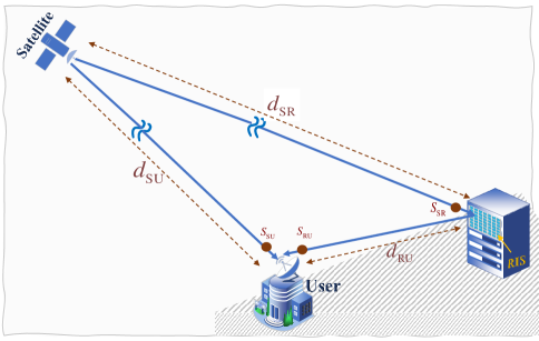
Figure 1: System model

The vector summation in (7) can be simplified to represent the overall magnitude and phase impact of each RIS. Formally, we can define: $\Gamma_{\mathrm{R}}=\sum_{n=1}^{N}\Gamma_{n}e^{-j\phi_{n}}$. Consequently,

$$S_{\mathrm{RU}}=\,\sqrt{\frac{G_{\mathrm{t}}G_{\mathrm{U}}\mathrm{\mathrm{G}_{\varphi_{\mathrm{sr}}}}\mathrm{G}_{\mathrm{\varphi_{\mathrm{ru}}}}}{L_{\mathrm{SR}}L_{\mathrm{RD}}}}\left|\Gamma_{\mathrm{R}}\right|e^{-j\left(\phi_{\mathrm{RU}}+\phi_{\mathrm{SR}}+\phi_{\mathrm{\mathit{R}}}\right)}.$$ (8)

Here, $\varphi_{\mathrm{sr}}$ and $\varphi_{\mathrm{ru}}$ are the common angles of incidence, $\left|\Gamma_{R}\right|$denotes the combined magnitude of individual reflection coefficients, and $\phi_{\mathrm{\mathit{R}}}$ represents the overall phase change due to the RIS. The total received power from both direct and reflected paths can be expressed as $P_{\mathrm{R}}=\left|S_{\mathrm{RU}}+S_{\mathrm{SU}}\right|^{2}$. This can be further simplified as follows

$$P_{\mathrm{R}}=P_{\mathrm{t}}\left|\sqrt{\frac{G_{\mathrm{u}}G_{\mathrm{t}}}{L_{\mathrm{SU}}}}e^{-j\phi_{\mathrm{SU}}}+\sqrt{\frac{G_{\mathrm{t}}G_{\mathrm{U}}\mathrm{\mathrm{G}_{\varphi_{\mathrm{sr}}}}\mathrm{G}_{\mathrm{\varphi_{\mathrm{ru}}}}}{L_{\mathrm{SR}}L_{\mathrm{RU}}}}\right.$$

$$\left.\left|\Gamma_{R}\right|e^{-j\left(\phi_{\mathrm{RU}}+\phi_{\mathrm{SR}}+\phi_{\mathrm{R}}\right)}\right|^{2}.$$ (9)

The expression for the received power $P_{\mathrm{R}}$ includes two paths, namely a direct path and a reflected path via the RIS. Each path is associated with a specific field strength, phase shift, and path loss. The direct path from the satellite $S$ to the user, U, is characterized by a complex amplitude of the electric field $A_{\mathrm{SU}}$ and phase shift $-\phi_{\mathrm{RU}}-\phi_{\mathrm{SR}}$. On the other hand, the reflected path via the RIS is characterized by a complex amplitude of the electric field $A_{\mathrm{RU}}$ and a total phase shift $-\left(\phi_{\mathrm{RU}}+\phi_{\mathrm{SR}}+\phi_{\mathrm{R}}\right)$. Note that these phase shifts are negative as they represent the shift experienced by the signal while traversing the respective paths. The complex amplitude $A_{\mathrm{SU}}$ and $A_{\mathrm{RU}}$ have been defined as follows:

$$A_{\mathrm{SU}}=P_{t}\sqrt{\frac{G_{\mathrm{u}}G_{\mathrm{t}}}{L_{\mathrm{SU}}}}$$ (10)

$$A_{\mathrm{RU}}=P_{t}\sqrt{\frac{G_{\mathrm{t}}}{L_{\mathrm{SR}}}}\sqrt{\mathrm{\mathrm{G}_{\varphi_{\mathrm{sr}}}}\mathrm{G}_{\mathrm{\varphi_{\mathrm{ru}}}}}\left|\Gamma_{\mathrm{R}}\right|\sqrt{\frac{G_{\mathrm{u}}}{L_{\mathrm{RU}}}}$$ (11)

We define two new phase terms, $\phi_{1}$ and $\phi_{2}$, where $\phi_{1}=-\phi_{\mathrm{SU}}$ and $\phi_{2}=-\left(\phi_{\mathrm{RU}}+\phi_{\mathrm{SR}}+\phi_{\mathrm{R}}\right).$ The minus signs here are due to the convention of treating outgoing signals as having a negative phase. Now, the total received signal is $A_{\mathrm{SU}}e^{\phi_{1}}+A_{\mathrm{RU}}e^{\phi_{2}}.$ The received power $P_{\mathrm{R}}$ is then the square of the magnitude of the total received signal, then (13) can be re-expressed as

$$P_{\mathrm{R}}=\,\left|A_{\mathrm{SU}}e^{\phi_{1}}+A_{\mathrm{RU}}e^{\phi_{2}}\right|^{2}$$ (12)

Convert the exponential parts in (12) using Euler’s formula, we get

$$P_{R}=P_{t}\,\left|A_{\mathrm{SU}}\left(\cos(\phi_{1})+j\sin(\phi_{1})\right)\right.$$

$$+\left.A_{\mathrm{RU}}\left(\cos(\phi_{2})+j\sin(\phi_{2})\right)\right|^{2}$$ (13)

By applying the formula for the square of the magnitude of a complex number, consider the absolute modulus of a complex number and using the trigonometric identity, (13) yielding as

$$P_{R}=P_{t}\left[A_{\mathrm{SU}}^{2}+A_{\mathrm{RU}}^{2}+2A_{\mathrm{SU}}A_{\mathrm{RU}}\cos(\phi_{1}-\phi_{2})\right]$$ (14)

Expression (14), captures the contributions to the received power from both the direct link (Satellite to User) and the reflected link (RIS to User), as well as their interference.

III Optimize $\phi_{\mathrm{R}}$ under ideal conditions

The objective of the proposed method is to optimize the phase shift $\phi_{\mathrm{R}}$ to maximize the power received $P_{R}$ at a given range distance $d_{\mathrm{RU}}$. By doing so, the coverage of a wide range of users or areas is achieved more effectively. Now, using expression (14), and rearrange $\phi_{1}$ and $\phi_{2}$ , we get

$$P_{R}(\phi_{\mathrm{R}})=P_{t}\left[A_{\mathrm{SU}}^{2}+A_{\mathrm{RU}}^{2}+2A_{\mathrm{SU}}A_{\mathrm{RU}}\cos(\phi_{\mathrm{\mathit{R}}}-\Theta)\right]$$ (15)

where $\Theta=\phi_{\mathrm{SU}}-\phi_{\mathrm{SR}}-\phi_{\mathrm{RU}}.$ Under ideal conditions where the influences of RIS and other communication factors between the transmitter and the receiver are assumed to be optimal, the objective of maximizing $P_{R}$ by finding the optimal value of $\phi_{\mathrm{R}}$ can be formulated as follows:

$$Maximize\,P_{R}(\phi_{\mathrm{R}})$$ (16)

$$\mathrm{s.t\quad 0\leq\phi_{R}\leq 2\pi}$$

To solve this optimization problem, we need to find the value of $\phi_{\mathrm{R}}$ that makes the derivative $\frac{dP_{R}}{d\phi_{R}}$ equal to zero, meaning there is no change in $P_{R}$ with a small change in $\phi_{\mathrm{R}}$. Mathematically, this condition is expressed by setting the derivative to zero:

$$0=\mathrm{-P_{S}}\left(A_{\mathrm{SU}}^{2}+A_{\mathrm{RU}}^{2}+2A_{\mathrm{SU}}A_{\mathrm{RU}}\sin(\phi_{\mathrm{R}}-\Theta)\right),$$ (17)

Solving the equation yields that sin$(\phi_{R}-\Theta)=0$. The sin function equals zero at multiples of $\pi$, therefore we can set $\phi_{R}-\Theta=\pi\mathfrak{n}$, where $\mathfrak{n}$ is an integer representing the number of complete cycles around the unit circle. Consequently, we can express $\phi_{R}$ as:

$$\phi_{R}=\Theta+\pi\mathfrak{n}\text{ for }\mathfrak{n}\in\mathbb{Z}$$ (18)

This equation gives all possible values of $\phi_{R}$ that satisfy sin$(\phi_{R}-\Theta)=0.$ Notably, each phase component in $\Theta$ is influenced linearly by the corresponding distance, with $\Theta$ being particularly sensitive to changes in $d_{\mathrm{RU}}$. As such, any variations in $d_{\mathrm{RU}}$ result in changes to the optimal value of$\phi_{R}$ needed to maximize the received power. Moreover, the maximization of $P_{R}$ also involves a constraint on the range of $\phi_{R}$, which limits it to the interval [$0,2\pi$]. To ensure that $\phi_{R}$ always falls within this interval, even if $\Theta$ does not, we employ the modulo operation. Therefore, the optimal solution for $\phi_{R}$, denoted as $\overset{*}{\phi}_{R}$, can be expressed as:

$$\overset{*}{\phi}_{R}=\Theta-2\pi\left\lfloor\frac{\Theta}{2\pi}\right\rfloor$$ (19)

Here, $\lfloor.\rfloor$ denotes the floor function, which returns the largest integer less than or equal to its argument. In this case, it subtracts the largest multiple of $2\pi$ that is less than or equal to $\Theta$ from $\Theta$ itself, ensuring that the resulting $\phi_{R}$ falls within the required range [$0,2\pi$]. The plot in Fig. 2 shows a 3D surface plot, representing how the total received power $P_{R}$ changes with both the distance from the RIS to the user $d_{\mathrm{RU}}$ and the phase shift at the RIS $\phi_{R}$. The horizontal axes (x and y) represent $d_{RU}$ and $\phi_{R}$ respectively, and the vertical axis ($z$) represents $P_{R}$. The coloured surface thus gives us a way of visualizing how $P_{R}$ varies across a range of $d_{\mathrm{RU}}$ and $\phi_{R}$ values. Each point on the surface corresponds to a specific combination of $d_{\mathrm{RU}}$ and $\phi_{R}$, and the height of the point from the base plane indicates the value of $P_{R}$ for that combination. The colour of each point on the surface represents its $P_{R}$ value, with colours varying from dark blue (for the lowest $P_{R}$ values) to dark red (for the highest $P_{R}$ values). The colorbar on the side of the plot provides a guide to understanding what $P_{R}$ value each colour represents. In addition to the surface, we also have a line plot (the red line) superimposed on the surface. This line represents the optimal phase shift $\overset{*}{\phi}_{R}$ that maximizes $P_{R}$ for each $d_{\mathrm{RU}}$ value. The points on this line correspond to the points on the surface where $P_{R}$ reaches its maximum value for the corresponding $d_{\mathrm{RU}}$. So, in a nutshell, this plot helps us understand how $P_{R}$ varies with $d_{RU}$ and $\phi_{R}$, and it shows us the optimal $\phi_{R}$ values that maximize $P_{R}$ for each $d_{RU}$. The colour of the surface helps us quickly visualize the $P_{R}$ value at any given combination of $d_{RU}$ and $\phi_{R}$, and the red line helps us see the optimal $\phi_{R}$ values at a glance.

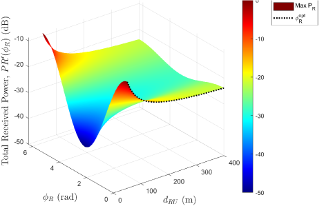
Figure 2: Total received power with RIS as a function of $d_{RU}$ and $\phi_{R}$

In Fig. 3, comparing the two distinct scenarios that are plotted: one with the aid of an RIS and another without its involvement. The $x$-axis of the graph represents the distance from the RIS to the user, termed as $d_{\mathrm{RU}}$. This axis effectively maps the changing physical proximity between the RIS and the user. On the other hand, the $y$-axis denotes the total received power, denoted as $P_{R}$. The first scenario, delineated by the red line, showcases a system devoid of an RIS. Interestingly, in this setup, the received power at the user’s end remains constant, irrespective of any changes in the distance $d_{\mathrm{RU}}$. This serves to highlight the limitations of a system lacking the deployment of an RIS, with its inability to capitalize on the user’s proximity for improving the received power. Contrastingly, the second scenario, depicted by the blue line, incorporates the role of an RIS in the system. This plot clearly exhibits a correlation between the distance $d_{\mathrm{RU}}$ and the total received power $P_{R}$. Here, the total power received by the user evidently increases with the optimal adjustment of the RIS’s phase shift at closer distances. The graphical comparison plot underscores the pivotal role of a RIS in leveraging spatial context to enhance the total power received by the user. The contrast between the two scenarios emphasizes the substantial advantages of incorporating a RIS into the system, particularly its capability to adapt dynamically to the user’s location and optimize the received power.

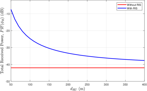
Figure 3: Comparison of total received power with and without RIS

IV $\mathit{P_{R}}$ under non-ideal conditions $\phi_{\mathrm{R}}$

The preceding section discussed the optimization of phase shift values ($\phi_{R}$) under ideal network conditions. However, in real-world scenarios, non-ideal situations arise, introducing phase errors in reconfigurable intelligent surfaces (RISs) [16]. These errors can originate from various factors such as hardware imperfections, quantization errors, channel condition or calibration inaccuracies, significantly impacting the received signal and overall system performance [32]. To account for these challenges in the received power equation (14), we, can rearrange the phases in equation (14) as assume that the main error primarily affects the phase component of the signal . Now, to incorporate the phase errors into (14), the phase $(\phi_{1}-\phi_{2})$ can be modeled considering an error effect ($\delta)$. The error factor $\delta$ can be perceived as an additive or multiplicative error [33]. The additive error model assumes that the phase error adds to the desired phase; thus, the RIS-added phase is $(\phi_{1}-\phi_{2})+\delta$. Conversely, the multiplicative error model postulates that the phase error multiplies the desired phase, rendering the RIS-added phase as $(\phi_{1}-\phi_{2})(1+\delta)$. The chosen model should fit the system better according to the RIS application. Both models can spur intricate mathematical analysis, typically beginning with statistical properties of the phase error (such as mean and variance), using them to derive the statistical properties of the received signal or the system performance metric of interest (such as Signal-to-Noise Ratio ), Bit Error Rate (BER), etc). However, the additive error model, indicative of phase shift or perturbation is more commonly used [33]. Therefore, our proposed mathematical model that considers phase errors adopts the additive error model. Assume the phase errors follows a uniform distribution in the interval $[-\sigma,\sigma]$, denoted as $\delta\sim\mathcal{U}(-\sigma,\sigma)$. The uniform distribution is characterized by its mean ($\mu$) and variance ($\sigma^{2}$), and its probability density function (PDF) is given by:

$$f(\delta)=\begin{cases}\frac{1}{2\sigma},&\text{if }-\sigma\leq\delta\leq\sigma\\ 0,&\text{otherwise}\end{cases}$$ (20)

Since the phase errors are modelled as a random variable with a known distribution, the expectation value of $P_{\mathrm{R}}(\Phi_{1})$ can be applied to examine the phase error’s impact on system performance. The expectation value is given as

$$E\left[P_{\mathrm{R}}\right]=P_{S}\left(A_{\mathrm{SU}}^{2}+A_{\mathrm{RU}}^{2}+2A_{\mathrm{SU}}A_{\mathrm{RU}}\>E\left[\cos\bigl{(}\phi_{1}-\phi_{2}+\delta\bigr{)}\right]\right),$$ (21)

where $E\left[.\right]$ is the expectation symbol which is effect only on $\cos\bigl{(}\phi_{1}-\phi_{2}+\delta\bigr{)}$ when we want to find the expectation of $P_{\mathrm{R}}$ over all phase errors $\delta$. The challenge here is that the expectation of a non-linear function of a random variable i.e., cosine of a random variable. However, we can apply the law of the unconscious statistician (LOTUS), which states that if g(x) is a function of a random variable $X$, then $E[g(X)]=\intop g(x)f_{X}(x)dx$, where $f_{X}(x)$ is the PDF of $X$. Using LOTUS for the cos term (21) as follows

$$E\left[\cos\bigl{(}\phi_{1}-\phi_{2}+\delta\bigr{)}\right]=\frac{1}{2\sigma}\intop_{-\sigma}^{\sigma}\cos\bigl{(}\phi_{1}-\phi_{2}+\delta\bigr{)}\>d\delta.$$ (22)

This gives

$$E\left[P_{\mathrm{R}}\right]=P_{S}\left(A_{\mathrm{SU}}^{2}+A_{\mathrm{RU}}^{2}+2A_{\mathrm{SU}}A_{\mathrm{RU}}\right.\>$$

$$\left.\frac{1}{2\sigma}\left[\sin\bigl{(}\phi_{1}-\phi_{2}+\sigma\bigr{)}-\sin\bigl{(}\phi_{1}-\phi_{2}-\sigma\bigr{)}\right]\right)$$ (23)

Further simplifying (23) is obtained by applying the trigonometric identity for the difference between two sine functions. This gives

$$E\left[P_{\mathrm{R}}\right]=P_{S}\left(A_{\mathrm{SU}}^{2}+A_{\mathrm{RU}}^{2}+2A_{\mathrm{SU}}A_{\mathrm{RU}}\>\mathrm{sinc}(\sigma)\cos(\phi_{1}-\phi_{2})\right)$$ (24)

where $\mathrm{sinc}$ is the sine cardinal function and it is defined as

$$\text{sinc}\,\sigma\equiv\left\{\begin{array}[]{cc}1&\text{ for }\sigma=0\\ \frac{\sin\sigma}{\sigma}&\text{ otherwise,}\end{array}\right.$$ (25)

So the term $\text{sinc}\,\sigma$ in Equation (23) provides an insight into how phase errors influence the system’s performance. This can be shown in Fig. 4, when the magnitude of the error (i.e., $\sigma$) equals zero, there is no error, and $\text{sinc}\,\sigma$ equals 1. This means that the effect of the cosine term in the expected power equation is at its maximum. As $\sigma$ increases (meaning the error gets larger), $\text{sinc}\,\sigma$ starts decreasing. As $\text{sinc}\,\sigma$ oscillates and gradually decreases as $\sigma$ moves away from zero, this implies that the larger the phase error, the smaller the $\mathrm{sinc}$ function, and thus the smaller the effect of the cosine term in your expected power equation. This decrease will be most significant when $\sigma$ starts to increase but will decrease less dramatically for larger $\sigma$ because of the sinc function’s shape (it oscillates and approaches zero as $\sigma$ goes to infinity, but the oscillations become less significant). This indicates that phase errors reduce the contribution of the constructive interference term in the power equation. However, due to the nature of the $\mathrm{sinc}$ function, small phase errors have a more noticeable impact than large ones.

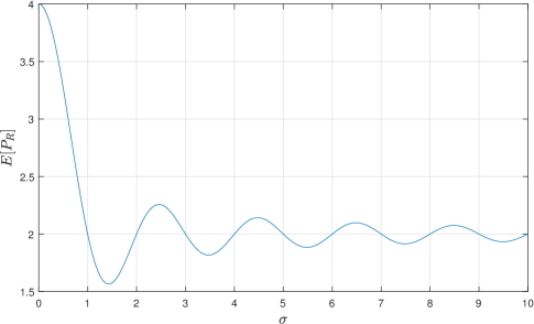
Figure 4: Impact of phase errors on received power

Figure 5 represents a 3D plot showing the relationship between the expected received power $E\left[P_{\mathrm{R}}\right]$, the RIS phase shift $\phi_{R}$ (which is a a part of $\phi_{2})$, and the phase error value ($\sigma$). The diagram reveals that as the phase error $\sigma$ increases, the received power $E\left[P_{\mathrm{R}}\right]$ correspondingly decreases. This can be attributed to the interference caused by the phase error between the desired signal and the reflected signal at the destination. Moreover, the plot reveals that certain values of phase shift $\phi_{R}$ can counterbalance the negative impacts of phase error and augment the received power. These particular phase shift values facilitate the alignment of the desired and reflected signals at the destination, causing constructive interference and consequently increasing the received power. Through the analysis of this 3D plot, we can comprehend how various combinations of phase shifts and phase errors influence the received power. Such understanding is pivotal in the context of system performance evaluation and understanding the resilience of the system to phase errors.

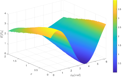
Figure 5: Relationship between $\phi_{R}$, $\sigma$, and $E[P_{R}]$

V Optimize $\phi_{\mathrm{R}}$ under non-ideal conditions

As delineated in section III, the optimization of phase shift values for RIS networks is traditionally applied under ideal conditions. However, with the introduction of non-ideal conditions expounded upon in section V, we are necessitated to augment our received power equation to encompass phase errors. These errors, treated as random variables, adhere to a uniform distribution thereby adding complexity to the optimization of the expected received power, $E[P_{R}]$. This transition engenders a shift in the optimization problem from determining a deterministic optimal phase shift value, $\phi_{R}$, to identifying an optimal $\phi_{R}$ that maximizes the expected received power, taking into account all plausible phase error values. To confront this complexity, stochastic optimization is proposed as a viable approach. In the realm of stochastic optimization, the objective function, denoted as $E[P_{R}]$ in our context, is characterized as a random variable. The aim, in this case, is to maximize its expected value as opposed to direct optimization. This leads us to formulate our stochastic optimization problem as:

$$\underset{\mathrm{0\,\leq\phi_{R}\leq 2\pi}}{\mathrm{max}}\left\{E[P_{R}(\phi_{R})]\right\}=\int_{-\sigma}^{\sigma}P_{R}(\phi_{R},\delta)f(\delta)\,d_{\delta}$$ (26)

where $P_{R}(\phi_{R},\delta)$ embodies the received power, inclusive of the phase shift value $\phi_{R}$ and the phase error $\delta$. Additionally, $f(\delta)$ denotes the probability density function of the phase error $\delta$, conforming to a uniform distribution.

To tackle the aforementioned problem, we apply the Monte Carlo method, a statistical technique that inherently consists of four steps. The first step, Monte Carlo Sampling, involves the generation of a set of $K$ samples for the random phase error $\delta$, represented as $\left\{\delta_{1},\delta_{2},...,\delta_{K}\right\}$. Each $\delta_{i}$ is independently drawn from the uniform distribution $\mathcal{U}(-\sigma,\sigma)$. The second step is the computation of the received power for each sample. For a specified phase shift $\phi_{R}$, we calculate the received power $P_{R}(\phi_{R},\delta_{i})$ for each sample $\delta_{i}$. This is accomplished using the formula

$$P_{R}(\phi_{R},\delta_{i})=P_{S}(A_{SU}^{2}+A_{RU}^{2}+2A_{SU}A_{RU}\text{sinc}(\sigma)\cos(\phi_{\mathrm{\mathit{R}}}-\Theta+\delta_{i}))$$ (27)

Once we have computed the received power for each sample, the third step is the estimation of the expected received power. This is performed by calculating the average over all samples, represented by the formula

$$E[P_{R}]\approx\frac{1}{K}\sum_{i=1}^{K}P_{R}(\phi_{R},\delta_{i})$$ (28)

The final stage in this process is the optimization of the phase shift. The objective here is to ascertain the phase shift $\phi_{R}$ that optimizes the estimated expected received power. This optimization of the problem can be formally represented as

$$\phi_{R}^{*}=\arg\max_{\phi_{R}}E[P_{R}]$$ (29)

Input: $K$ samples, Uniform distribution $\mathcal{U}(-\sigma,\sigma)$, Phase shift $\phi_{R}$

Output: Optimal phase shift $\phi_{R}^{*}$ that maximizes the estimated expected received power

for $i=1$ to $K$ do

       // Generate samples for phase error

       Draw $\delta_{i}$ independently from $\mathcal{U}(-\sigma,\sigma)$;

      

end for

for $i=1$ to $K$ do

       // Compute received power for each sample

       Compute $P_{R}(\phi_{R},\delta_{i})$ using $P_{S}(A_{SU}^{2}+A_{RU}^{2}+2A_{SU}A_{RU}\text{sinc}(\sigma)\cos(\phi_{R}-\Theta+\delta_{i}))$;

      

end for

// Estimate expected received power

Compute $E[P_{R}]$ using $E[P_{R}]\approx\frac{1}{K}\sum_{i=1}^{K}P_{R}(\phi_{R},\delta_{i})$;

// Optimize phase shift

Find $\phi_{R}^{*}$ using $\phi_{R}^{*}=\arg\max_{\phi_{R}}E[P_{R}]$;

Algorithm 1 Monte Carlo Estimation of Expected Received Power

The (29) problem can be solved using numerical optimization methods, as the exact analytical solution may be challenging to obtain due to the integral in the expected power and the stochastic nature of $\delta$. It’s noteworthy that larger $K$ generally leads to a more accurate estimation but incurs increased computational costs. Thus, a balance between accuracy and computational complexity should be considered. One common method is the Broyden–Fletcher–Goldfarb–Shanno (BFGS) algorithm, which is a powerful iterative method used to solve nonlinear optimization problems, and in our case, to optimize the phase shift $\phi_{R}$ for maximizing the expected received power $E[P_{R}]$. The algorithm starts with an initialization phase, where the initial guess for the phase shift $\phi_{R}$ is set to $\phi_{R}{}_{0}$. An initial approximation of the Hessian matrix, denoted as $H_{0}$, is also chosen, along with a convergence tolerance $\epsilon$, which helps stop the optimization when the change in$\phi_{R}$ becomes negligible. The main loop of the algorithm begins by computing the objective function, which, in this case, is the expected received power $E[P_{R}]$ for the current value of $\phi_{R}$. Following this, the gradient of the objective function with respect to $\phi_{R}$, denoted as $\nabla E[P_{R}]$, is computed. This gradient is an essential part of the update rule for $\phi_{R}$.

To update $\phi_{R}$, the BFGS algorithm computes the search direction using the formula

$$d_{j}=-H_{j}^{-1}\nabla E[P_{R}].$$ (30)

Here, $H_{j}^{-1}$ is the inverse of the current approximation to the Hessian matrix and $\nabla E[P_{R}]$ is the current gradient, and $j$ is the variable used as an iteration counter. The value of $\phi_{R}$ is then updated using the calculated search direction and a chosen step size $\alpha$, with the formula $\phi_{R}{}_{j+1}=\phi_{R}{}_{j}+\alpha d_{j}$. In the next step, a direction vector $s_{j}$ is computed, tracking the change in $\phi_{R}$ with the formula $s_{j}=\phi_{R}{}_{j+1}-\phi_{R}{}_{j}$. Alongside this, the step size $\alpha$ is determined. This step size should satisfy the Wolfe conditions or other line search criteria to ensure a sufficient reduction in the objective function. Once the direction vector and step size are calculated, the algorithm updates the approximation of the Hessian matrix, $H_{j+1}$, which is central to the BFGS method. The change in the gradient, $y_{j}$, is calculated as

$$y_{j}=\nabla E[P_{R}]_{j+1}-\nabla E[P_{R}]_{j}.$$ (31)

The Hessian approximation is then updated using the BFGS formula:

$$H_{j+1}=H_{j}+\frac{y_{j}y_{j}^{T}}{y_{j}^{T}s_{j}}-\frac{H_{j}s_{j}s_{j}^{T}H_{j}}{s_{j}^{T}H_{j}s_{j}}$$ (32)

This new Hessian approximation is used in the next iteration of the algorithm. The algorithm then checks for convergence. The convergence criteria could be the norm of the gradient becoming sufficiently small or the change in the objective function becoming negligible. If these criteria are satisfied, the optimization terminates. Otherwise, the algorithm returns to the beginning of the loop, repeating the process with the updated values of $\phi_{R}$, the gradient, and the Hessian approximation matrix. The termination of the algorithm results in the final value of $\phi_{R}$, which is the optimized solution $\phi_{R}^{*}$ that maximizes the expected received power. It’s important to underline that the efficiency and accuracy of the BFGS algorithm heavily depends on several factors such as the choice of the step size, the method for handling any constraints or regularization, and the careful initialization of the algorithm.

Input: $\phi_{R_{0}}$: Initial guess for $\phi_{R}$; $H_{0}$: Initial approximation of the Hessian matrix; $\epsilon$: Convergence tolerance

Output: $\phi_{R}^{*}$: Optimized value of $\phi_{R}$

Initialize: $j\leftarrow 0$;

while not converged do

       Compute the objective function $E[P_{R}]$ for $\phi_{R_{j}}$;

       Compute the gradient $\nabla E[P_{R}]$ for $\phi_{R_{j}}$;

       Compute the search direction: $d_{j}\leftarrow-H_{j}^{-1}\nabla E[P_{R_{j}}]$;

       Choose the step size $\alpha_{j}$ using line search;

       Update $\phi_{R_{j+1}}\leftarrow\phi_{R_{j}}+\alpha_{j}d_{j}$;

       Compute the direction vector: $s_{j}\leftarrow\phi_{R_{j+1}}-\phi_{R_{j}}$;

       Compute the change in gradient: $y_{j}\leftarrow\nabla E[P_{R_{j+1}}]-\nabla E[P_{R_{j}}]$;

       Update the Hessian approximation: $H_{j+1}\leftarrow H_{j}+\frac{y_{j}y_{j}^{T}}{y_{j}^{T}s_{j}}-\frac{H_{j}s_{j}s_{j}^{T}H_{j}}{s_{j}^{T}H_{j}s_{j}}$;

       $j\leftarrow j+1$;

      

end while

$\phi_{R}^{*}\leftarrow\phi_{R_{j}}$;

Algorithm 2 BFGS Algorithm for Optimizing $\phi_{R}^{*}=\arg\max_{\phi_{R}}E[P_{R}]$

Figure 6 presents a visual exploration of the impact of the phase shift ($\phi_{R}$) on the expected received power ($E[P_{R}]$), under varying levels of phase error standard deviation ($\sigma$). The expected received power is depicted as a function of the phase shift, and the plots are constructed for three distinct sigma values, which correspond to different degrees of phase error. In the figure, the x-axis represents the phase shift $\phi_{R}$ in radians, and the y-axis represents the expected received power $E[P_{R}]$. The curves clearly indicate that the expected received power is not uniform across the range of phase shifts but reaches a peak at certain optimal points. These peaks are marked by red circles, representing the optimal phase shifts that yield the maximum expected received power for the respective sigma values. The figure illustrates the sensitivity of the system’s performance to variations in the phase shift. It can be observed that the optimal phase shift for maximizing the expected received power varies with the degree of phase error standard deviation, indicating the interplay between the phase shift and phase error in determining system performance. Notably, as the phase error standard deviation increases, the optimal phase shift that maximizes the expected received power also changes. This analysis offers valuable insights into the optimization of phase shifts in the presence of phase errors. It reveals that for different levels of phase error standard deviation, different phase shifts might be optimal for achieving the maximum expected received power. These findings emphasize the importance of considering phase error characteristics in the design and optimization of phase shift-based communication systems, shedding light on system behavior under non-ideal conditions.

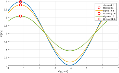
Figure 6: Optimization of total received power with varying phase shift

Fig. 7 presents the expected received power $E[P_{R}]$ as a function of the standard deviation of phase error sigma. Two distinct lines are plotted, representing the optimal and suboptimal cases of phase shift optimization. The x-axis of the plot corresponds to the values of sigma, representing the standard deviation of phase error introduced in the system. It ranges from a small non-zero value to a larger one, indicating an increasing level of phase error deviation. The y-axis represents the expected received power, which is the average power expected at the receiver given a particular phase shift. This is a critical parameter, as it directly influences the performance and reliability of the wireless communication system. The first line plot (labelled as ’Optimal Case’) illustrates the maximum expected received power for each value of sigma. It provides a clear picture of how phase shift optimization can improve the received power under various levels of phase errors. It reveals the best-case scenario for the system when the phase shift is optimally chosen to maximize the received power. The second line plot (labelled as ’Suboptimal Case’) shows the expected received power immediately before the maximum is reached for each value of sigma, and this case is illustrated in the 4. This presents the system’s performance just before the optimal phase shift is applied, essentially demonstrating the system’s performance under near-optimal conditions. By comparing these two lines, the plot clearly illustrates the improvements gained from optimal phase shift selection. It demonstrates how phase shift optimization helps in maintaining a higher expected received power even when the system is subjected to phase errors. The plot effectively underscores the significance of phase shift optimization in the performance of a wireless communication system subjected to phase errors. As a result, this plot serves as a vital tool for system designers, offering valuable insights into how phase errors and phase shift optimizations impact the performance of a wireless communication system.

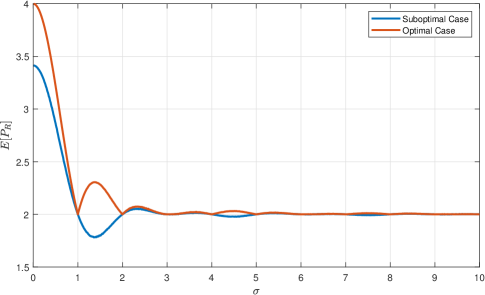
Figure 7: Relationship between Phase Error and Optimal $P_{R}^{\boldsymbol{{}^{\prime}}}$

VI Conclusion

This study investigated the application and optimization of Reconfigurable Intelligent Surfaces (RISs) in satellite communication systems, shedding light on the potential of RIS technology in enhancing system performance. The study’s central focus was the optimization of phase shift values, a crucial component of RIS functionality. To this end, we proposed novel methods that simplified the process under ideal conditions, resulting in more efficient and tractable solutions. However, recognizing that real-world scenarios often deviate from ideal conditions, we also accounted for the potential presence of phase errors. These errors can introduce substantial challenges to the received signal quality and overall system performance. In response, we extended our optimization framework to encompass these phase errors, demonstrating the robustness of our approach even in non-ideal conditions. The utilization of the Monte Carlo method and the BFGS algorithm was instrumental in our proposed solution. These tools allowed us to iteratively optimize the phase shift values while effectively handling the introduced uncertainties. The inclusion of these advanced methods in our study reinforces the practical feasibility and applicability of our approach. Through numerous illustrative examples, we showed that our proposed strategies can effectively optimize the system performance in various scenarios. Furthermore, the insights derived from the impact of phase errors provide valuable guidance for the design and optimization of future RIS-enhanced satellite communication systems. Overall, our work highlights the potential and flexibility of RISs in satellite communication systems and proposes robust strategies for optimizing their performance under a range of conditions. The findings serve as a solid foundation for further exploration and advancement in this emerging field, enabling the development of more efficient and reliable satellite communication systems.

References

- [1] Y. Seyedi, M. Shirazi, A. Moharrer, S. M. Safavi, and H. Amindavar, “Use of shadowing moments to statistically model mobile satellite channels in urban environments,” IEEE Transactions on Wireless Communications, vol. 12, no. 8, pp. 3760–3769, 2013.
- [2] A. Al-Hourani and I. Guvenc, “On modeling satellite-to-ground path-loss in urban environments,” IEEE Communications Letters, vol. 25, no. 3, pp. 696–700, 2021.
- [3] B. Evans, M. Werner, E. Lutz, M. Bousquet, G. Corazza, G. Maral, and R. Rumeau, “Integration of satellite and terrestrial systems in future multimedia communications,” IEEE Wireless Communications, vol. 12, no. 5, pp. 72–80, 2005.
- [4] E. Basar, M. Di Renzo, J. De Rosny, M. Debbah, M.-S. Alouini, and R. Zhang, “Wireless communications through reconfigurable intelligent surfaces,” IEEE Access, vol. 7, pp. 116 753–116 773, 2019.
- [5] M. A. ElMossallamy, H. Zhang, L. Song, K. G. Seddik, Z. Han, and G. Y. Li, “Reconfigurable intelligent surfaces for wireless communications: Principles, challenges, and opportunities,” IEEE Transactions on Cognitive Communications and Networking, vol. 6, no. 3, pp. 990–1002, 2020.
- [6] Q. Wu and R. Zhang, “Towards smart and reconfigurable environment: Intelligent reflecting surface aided wireless network,” IEEE Communications Magazine, vol. 58, no. 1, pp. 106–112, 2020.
- [7] W. Tang, M. Z. Chen, X. Chen, J. Y. Dai, Y. Han, M. Di Renzo, Y. Zeng, S. Jin, Q. Cheng, and T. J. Cui, “Wireless communications with reconfigurable intelligent surface: Path loss modeling and experimental measurement,” IEEE Transactions on Wireless Communications, vol. 20, no. 1, pp. 421–439, 2021.
- [8] H. Ren, Z. Zhang, Z. Peng, L. Li, and C. Pan, “Energy minimization in ris-assisted uav-enabled wireless power transfer systems,” IEEE Internet of Things Journal, pp. 1–1, 2022.
- [9] S. Zhang and R. Zhang, “Capacity characterization for intelligent reflecting surface aided mimo communication,” IEEE Journal on Selected Areas in Communications, vol. 38, no. 8, pp. 1823–1838, 2020.
- [10] H. Chen, G. Yang, and Y.-C. Liang, “Joint active and passive beamforming for reconfigurable intelligent surface enhanced symbiotic radio system,” IEEE Wireless Communications Letters, vol. 10, no. 5, pp. 1056–1060, 2021.
- [11] S. V. Hum and J. Perruisseau-Carrier, “Reconfigurable reflectarrays and array lenses for dynamic antenna beam control: A review,” IEEE Transactions on Antennas and Propagation, vol. 62, no. 1, pp. 183–198, 2014.
- [12] K.-T. Nguyen, T.-H. Vu, and S. Kim, “Exploiting reconfigurable intelligent surface-based uplink/downlink wireless systems,” IEEE Access, vol. 10, pp. 91 059–91 072, 2022.
- [13] Y. Liu, X. Liu, X. Mu, T. Hou, J. Xu, M. Di Renzo, and N. Al-Dhahir, “Reconfigurable intelligent surfaces: Principles and opportunities,” IEEE Communications Surveys Tutorials, vol. 23, no. 3, pp. 1546–1577, 2021.
- [14] Y. Shang, Q. Zeng, W. Cui, X. Wang, and G. Zheng, “Design of pattern reconfigurable patch antenna array based on reflective phase-shifter,” International Journal of Antennas and Propagation, vol. 2022, pp. 1–10, 02 2022.
- [15] C. Pan, H. Ren, K. Wang, J. F. Kolb, M. Elkashlan, M. Chen, M. Di Renzo, Y. Hao, J. Wang, A. L. Swindlehurst, X. You, and L. Hanzo, “Reconfigurable intelligent surfaces for 6g systems: Principles, applications, and research directions,” IEEE Communications Magazine, vol. 59, no. 6, pp. 14–20, 2021.
- [16] W. Khalid, M. A. Ur Rehman, T. Van Chien, and H. Yu, “Simultaneously transmitting and reflecting-reconfigurable intelligent surfaces with hardware impairment and phase error,” in 2023 International Conference on Artificial Intelligence in Information and Communication (ICAIIC), 2023, pp. 654–656.
- [17] E. Björnson, Ö. Özdogan, and E. G. Larsson, “Reconfigurable intelligent surfaces: Three myths and two critical questions,” CoRR, vol. abs/2006.03377, 2020. [Online]. Available: https://arxiv.org/abs/2006.03377
- [18] G. C. Trichopoulos, P. Theofanopoulos, B. Kashyap, A. Shekhawat, A. Modi, T. Osman, S. Kumar, A. Sengar, A. Chang, and A. Alkhateeb, “Design and evaluation of reconfigurable intelligent surfaces in real-world environment,” IEEE Open Journal of the Communications Society, vol. 3, pp. 462–474, 2022.
- [19] W. Xu, Y. Cui, H. Zhang, G. Y. Li, and X. You, “Robust beamforming with partial channel state information for energy efficient networks,” IEEE Journal on Selected Areas in Communications, vol. 33, no. 12, pp. 2920–2935, 2015.
- [20] Y. Bian, D. Dong, J. Jiang, and K. Song, “Performance analysis of reconfigurable intelligent surface-assisted wireless communication systems under co-channel interference,” IEEE Open Journal of the Communications Society, vol. 4, pp. 596–605, 2023.
- [21] D. Li, “Ergodic capacity of intelligent reflecting surface-assisted communication systems with phase errors,” IEEE Communications Letters, vol. 24, no. 8, pp. 1646–1650, 2020.
- [22] I. Trigui, E. K. Agbogla, M. Benjillali, W. Ajib, and W.-P. Zhu, “Bit error rate analysis for reconfigurable intelligent surfaces with phase errors,” IEEE Communications Letters, vol. 25, no. 7, pp. 2176–2180, 2021.
- [23] W. Zhang, J. Xu, W. Xu, X. You, and W. Fu, “Worst-case design for ris-aided over-the-air computation with imperfect csi,” IEEE Communications Letters, vol. 26, no. 9, pp. 2136–2140, 2022.
- [24] X. Liu, Y. Yu, B. Peng, X. B. Zhai, Q. Zhu, and V. C. M. Leung, “Ris-uav enabled worst-case downlink secrecy rate maximization for mobile vehicles,” IEEE Transactions on Vehicular Technology, vol. 72, no. 5, pp. 6129–6141, 2023.
- [25] R. Li, S. Sun, Y. Chen, C. Han, and M. Tao, “Ergodic achievable rate analysis and optimization of ris-assisted millimeter-wave mimo communication systems,” IEEE Transactions on Wireless Communications, vol. 22, no. 2, pp. 972–985, 2023.
- [26] S. Ma, W. Shen, X. Gao, and J. An, “Robust channel estimation for ris-aided millimeter-wave system with ris blockage,” IEEE Transactions on Vehicular Technology, vol. 71, no. 5, pp. 5621–5626, 2022.
- [27] X. Yu, K. Yu, X. Huang, X. Dang, K. Wang, and J. Cai, “Computation efficiency optimization for ris-assisted millimeter-wave mobile edge computing systems,” IEEE Transactions on Communications, vol. 70, no. 8, pp. 5528–5542, 2022.
- [28] B. Zhao, M. Lin, S. Xiao, M. Cheng, W.-P. Zhu, and N. Al-Dhahir, “Robust beamforming for ris enhanced transmissions in cognitive radio networks,” IEEE Transactions on Vehicular Technology, vol. 72, no. 5, pp. 6800–6804, 2023.
- [29] Y. Xu, H. Xie, Q. Wu, C. Huang, and C. Yuen, “Robust max-min energy efficiency for ris-aided hetnets with distortion noises,” IEEE Transactions on Communications, vol. 70, no. 2, pp. 1457–1471, 2022.
- [30] D. Vallado and W. McClain, Fundamentals of Astrodynamics and Applications, ser. Fundamentals of Astrodynamics and Applications. Microcosm Press, 2001. [Online]. Available: https://books.google.com.au/books?id=OCkGmwEACAAJ
- [31] M. I. Khalil, “Enhancing active reconfigurable intelligent surface,” Intelligent and Converged Networks, vol. 3, no. 4, pp. 351–363, 2022.
- [32] I. Yildirim, A. Uyrus, and E. Basar, “Modeling and analysis of reconfigurable intelligent surfaces for indoor and outdoor applications in future wireless networks,” IEEE Transactions on Communications, vol. 69, no. 2, pp. 1290–1301, 2021.
- [33] G. Tang, “Characterization of the systematic and random errors in satellite precipitation using the multiplicative error model,” IEEE Transactions on Geoscience and Remote Sensing, vol. 59, no. 7, pp. 5407–5416, 2021.