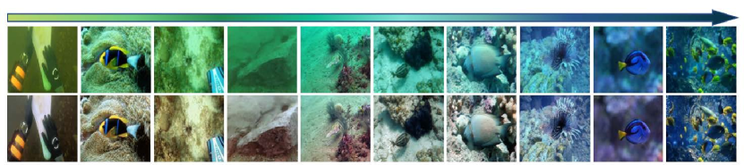
Figure 1. Visual results of our GUPDM on various underwater image types. The first row displays a series of degraded underwater images ranging from yellow to blue and the second row shows the enhanced results with our method.

A Generalized Physical-knowledge-guided Dynamic Model for Underwater Image Enhancement

Abstract.

Underwater images often suffer from color distortion and low contrast resulting in various image types, due to the scattering and absorption of light by water. While it is difficult to obtain high-quality paired training samples with a generalized model. To tackle these challenges, we design a Generalized Underwater image enhancement method via a Physical-knowledge-guided Dynamic Model (short for GUPDM), consisting of three parts: Atmosphere-based Dynamic Structure (ADS), Transmission-guided Dynamic Structure (TDS), and Prior-based Multi-scale Structure (PMS). In particular, to cover complex underwater scenes, this study changes the global atmosphere light and the transmission to simulate various underwater image types (e.g., the underwater image color ranging from yellow to blue) through the formation model. We then design ADS and TDS that use dynamic convolutions to adaptively extract prior information from underwater images and generate parameters for PMS. These two modules enable the network to select appropriate parameters for various water types adaptively. Besides, the multi-scale feature extraction module in PMS uses convolution blocks with different kernel sizes and obtains weights for each feature map via channel attention block and fuses them to boost the receptive field of the network. The source code will be available at https://github.com/shiningZZ/GUPDM.

1. Introduction

Due to the scattering and absorbing effects of the water on light, underwater images generally suffer from low contrast, color shift and blur. The quality of underwater images can directly or indirectly affect the accuracy of underwater robots in performing tasks such as detection, segmentation, tracking and classification. Therefore, Underwater Image Enhancement (UIE) plays an important role in underwater tasks.

The existing UIE methods can be coarsely divided into two categories: traditional and deep learning-based ones. Traditional UIE methods includes prior-based (Galdran et al., 2015; Drews et al., 2013; Akkaynak and Treibitz, 2018; Chiang and Chen, 2011; Li et al., 2016; Akkaynak and Treibitz, 2019a, b; Peng and Cosman, 2017; Wang et al., 2017) and model-free (Ancuti et al., 2012; Ghani and Isa, 2015; Ancuti et al., 2019; Iqbal et al., 2010; Zhang et al., 2017) approaches. Prior-based ones utilize rich priors and estimate the parameters of underwater image formation model to generate the enhanced images. For example, (Drews et al., 2013; Akkaynak and Treibitz, 2018; Chiang and Chen, 2011; Li et al., 2016) focus on the estimation of medium transmittance to restore underwater images. Although these methods make full use of prior information, they are less practical in complex scenarios, which often leads to over-enhancement of images and thus cannot be applied to real underwater scenes. Model-free methods often rely on the spatial relationship between pixel values of the original underwater image to improve the brightness, contrast and saturation of the image, such as Gray World (Buchsbaum, 1980), Max RGB (Land, 1977) and White Balance(Liu et al., 1995). However, these methods tend to ignore the details and depth information of the image, resulting in artifacts and poor adaptation to the complex underwater degradations.

Deep learning has introduced new strategies for UIE task (Li et al., 2020; Fu et al., 2022b; Li et al., 2021; Fu et al., 2022a; Mu et al., 2022; Guo et al., 2022; Huang et al., 2023; Jiang et al., 2022a; Liu et al., 2022a; Lin et al., 2021; Jiang et al., 2022b; Lin et al., 2021). Those methods can achieve complex non-systematic end-to-end modeling or combine physical priors with networks to solve the existing problems. These methods have better feature representation capacity, benefiting from large data they utilized to train. Hypernet (Ha et al., 2016; Lin et al., 2020; Yin et al., 2022; Liu et al., 2020b, 2022b) is one of the great works among deep learning-based approaches, which uses a relatively small network to generate weights for target network. These methods have better feature representation capacity, as they leverage large data to train. However, the main challenge is the high cost and difficulty of acquiring large-scale underwater datasets, which forces most methods to use small-scale datasets. Consequently, many GAN-based approaches focus on unsupervised UIE (Li et al., 2019b; Guo et al., 2019; Islam et al., 2020b; Fabbri et al., 2018; Jiang et al., 2022b) models, aiming to synthesize underwater images by learning a realistic representation of underwater conditions from unlabeled images. Nevertheless, a significant gap between the synthesized underwater images and the real ones still remains, in terms of plausibility and scene diversity.

Overall, we summarize the challenges existing in underwater image enhancement as follows. 1) Underwater images often suffer from color distortion and low contrast, due to the scattering and absorption of light by water. Moreover, the water quality and the distance of light transmission also affect the image clarity, making the underwater images blurry. 2) The scarcity of high-quality paired training samples constrains the performance of learning-based models. 3) Model generalization is a critical task for UIE task, which is important but has been neglected by many researches, as shown in Fig. 2. For example, a model obtained through training one dataset maybe not suitable for another water types.

Contributions: To tackle these challenges, this work designs a Generalized Underwater image enhancement method via Physical-knowledge-guided Dynamic Model (short for GUPDM), consisting of three parts: Atmosphere-based Dynamic Structure (ADS), Transmission-guided Dynamic Structure (TDS) and Prior-based Multi-scale Structure (PMS), as shown in Fig. 3. In particular, to cover complex underwater scenes, this study varies the global atmosphere and the transmission, reaching various underwater image types (e.g., the underwater image color ranging form yellow to blue) through the formation model. Then, we design a ADS that uses dynamic convolutions to adaptively extract prior information of underwater images and generate parameters for PMS. In addition, to force our model to pay more attention to various details in images, this work introduces a TDS to enable our network to adaptively select suitable parameters. Thus, the whole network can obtain appropriate parameters according to the water type of underwater image, making the proposed model more robust. Besides, the Multi-scale Feature Extraction (MFE) module in PMS uses convolution blocks with different kernel sizes and obtain weights for each feature map via channel attention block and then fuses them to boost the receptive field of network. We summarize the main contributions as follows:

• This work designs a generalized underwater image enhancement method via physical-knowledge-guided (i.e., various atmosphere and transmission) dynamic model to adaptively enhance the underwater images with different water types (as shown in Fig. 1).

• To cover complex underwater scene, by varying global atmosphere light, we design a ADS that uses dynamic convolutions to adaptively extract prior information of underwater images and generates parameters for base network structure. This also allows the entire model to adjust the parameters according to the degradation level of input image, improving the generalization capacity of network.

• The proposed TDS uses medium transmittance-based prior to prompt the network to pay more attention to areas with the most quality degradation, enabling the network to adaptively select appropriate parameters according to water quality.

• Extensive experiments demonstrate that our method achieves superior performance and the best generalization capacity, reaching the state-of-the-art level on multiple test datasets.

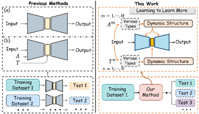
Figure 2. Schematic description of previous deep-learning methods (left) and our model (right).

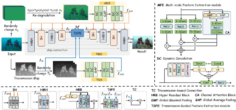
Figure 3. Overall illustration of the proposed GUPDM framework. GUPDM is composed of three components: Atmosphere-based Dynamic Structure (ADS), Transmission-guided Dynamic Structure (TDS) and Prior-based Multi-scale Structure (PMS).

2. Related Works

We briefly review previous related works regarding the traditional UIE models and deep learning-based UIE approaches.

Traditional UIE Models: The Traditional UIE Models can be summarized as prior-based approaches and model-free approaches. The prior-based approaches are grounded on physical model intended to estimate the parameters of underwater image formation model by using visual cues and then reconstruct a clean image by applying these parameters in reverse. For instance, in (Galdran et al., 2015), researchers propose a variant of DCP which uses red channel information to estimate the transmission map of underwater images. UDCP (Drews et al., 2013) estimates the transmission map by considering the blue and green color channels. Moreover, Sea-thru (Akkaynak and Treibitz, 2019a) estimates the back scatter and attenuation coefficient by using RGBD images as input.

Another type of traditional methods is model-free approach which improve the chromatic aberration and contrast by modifying the overall pixel values of underwater images, including histogram equalization (Pizer, 1990), white balance (Liu et al., 1995) and Retinex (Rahman et al., 1996). To fully enhance the image details and colors, (Ghani and Isa, 2015) proposes a method that integrates global and local contrast stretching. To handle the artifacts caused by the severely uneven color spectrum distribution, 3C (Ancuti et al., 2019) reconstructs the lost channel based on opponent color. These traditional methods can improve the visual effect to some extent. However, these methods may result in color distortions and artifacts when encountered with sophisticated illumination conditions.

UIE Approaches based on Deep-learning: Deep learning methods are trained on large scale underwater images and can automatically extract relevant features from them to improve the quality of enhanced images. For example, methods use Generative Adversarial Network (GAN) for image enhancement includes FGAN (Li et al., 2019b), DenseGAN (Guo et al., 2019), UGAN (Fabbri et al., 2018) and FUnIE-GAN (Islam et al., 2020b). The main purpose of GAN strategy is to expand the source of pairing data through generative networks, but there is still a lack of high-quality training samples that truly match real underwater scenarios and diverse degradation. Due to the nonavailability of ground truth high-quality images, a novel probabilistic network PUIE-Net (Fu et al., 2022b) is proposed to learn the enhanced distribution of degraded underwater images. These end-to-end methods can produce visually pleasing results. However, they usually require a specific model for each dataset and lack generalization ability and flexibility in handling different underwater scenarios, due to the complexity of underwater environments. The methods trained on real data can produce visually pleasing results. However, they cannot restore the color and structure of specific objects well and tend to produce inauthentic results since the reference images are not the actual ground truths. To tackle these problems, some models (Liu et al., 2019, 2018; Li et al., 2020, 2021; Qian et al., 2022) integrate the priors like transmission map and atmosphere light to deal with the environmental information. For instance, UWCNN (Li et al., 2020) is trained on synthesize datasets with underwater scene prior. Instead of estimating the parameters of underwater imaging model, UWCNN directly reconstructs clear enhanced images. Ucolor (Li et al., 2021) uses medium transmission-guided multi-color embedding to solve the color casts and low contrast issues. DDNet (Qian et al., 2022) uses medium transmission maps and global atmosphere light to form the haze and scene-adaptive convolutions.

3. Our Developed Framework

This section detailed introduces the developed framework as shown in Fig. 3. Subsection 3.1 first present the motivation and the problem formulation of this work. Subsection 3.2 describes the detailed structure of GUPDM and Subsection 3.3 presents the loss functions and training procedure.

3.1. Motivation and Problem Formulation

Following Akkaynak’s light scattering model (Akkaynak and Treibitz, 2019a), the degraded underwater images can be expressed as

(1) $$\mathbf{I}_{c}(x)=\mathbf{J}_{c}(x)e^{-\bm{\beta}d(x)}+\left(1-e^{-\bm{\beta}d(x)}\right)\mathbf{A}_{c},c\in\{r,g,b\}$$

where $x$ indicates the spatial location of each pixel, $\mathbf{I}_{c}$ is the observed image, $\mathbf{J}_{c}$ is the restored haze-free image and $\mathbf{A}_{c}$ means the global background light, $d(x)$ is the scene depth at pixel $x$ and $\bm{\beta}$ is the channel-wise extinction coefficient depending on the water quality. $\mathbf{T}_{c}(x):=e^{-\bm{\bm{\beta}}d(x)}$ is the medium transmission map representing the percentage of scene spoke brightness that reaches the camera after reflection from point $x$ in the underwater scene, which also reflect the water type.

Due to the color cast caused by varying light attenuation with different wavelengths and haze effect caused by scattering, there exist various types of degraded underwater images (see Fig. 4). In other words, we can roughly simulate complex underwater scene with the global atmosphere light $\mathbf{A}_{c}$ and the transmission map $\mathbf{T}_{c}$. Inspired by aforementioned information, we change the original input underwater images by adjusting the two parameters. We aim to reduce the color cast of underwater images through making such changes so that our encoders can learn more information about the color. This operation can also help to augment the data to better handle the deficient data problem of underwater image. Thus, we generate the input images as is shown in Fig. 4. We summarize the re-degradation types as $\mathbf{I}_{c}(x)\stackrel{{\scriptstyle(a),(b)}}{{\longrightarrow}}\mathbf{I}_{c}^{m,n}(x)$, where

• Varing $\mathbf{A}_{c}\to\mathbf{A}_{c}^{m}$, based on Eq. (1), we obtain $\mathbf{I}_{c}^{m}(x)$;

• If we further vary $\mathbf{T}_{c}(x)\to\mathbf{T}_{c}^{n}(x)$, we obtain $\mathbf{I}_{c}^{n}(x)$.

Motivated by the above analysis, this work aims to restore various underwater images using a generalized model. Therefore, the key is to enable the designed network ot estimate the features of varied types. We design an Atmosphere-based Dynamic Structure $\mathcal{A}$ (i.e., ADS) and a Transmission-based Dynamic Structure $\mathcal{T}$ (i.e., TDS) to jointly guide the Prior-based Multi-scale Structure $\mathcal{N}$ (i.e., PMS). Actually, the $\mathcal{N}$ acts as a base network structure for UIE while $\mathcal{A}$ and $\mathcal{T}$ are two hyper-guided modules with different level. Thus, we formulate this problem in the following forms:

(2) $$\begin{array}[]{l}\min\limits_{\bm{\theta},\bm{\phi}}L\left(\widehat{\mathbf{J}}_{c}(x),\bar{\mathbf{J}}_{c}(x);\mathbf{I}_{c}^{m}(x),\mathbf{I}_{c}^{n}(x)\right)\\ s.t.,\bm{\omega}\in\arg\min\limits_{\bm{\omega}}F(\widetilde{\mathbf{J}}_{c}(x);\mathbf{I}_{c}(x)),\end{array}$$

where $\bm{\theta},\bm{\phi}$ and $\bm{\omega}$ are the parameters of module ADS, TDS and PMS, respectively; $L$ and $F$ are the loss functions; $\widetilde{\mathbf{J}}_{c}(x)$, $\widehat{\mathbf{J}}_{c}(x)$ and $\bar{\mathbf{J}}_{c}(x)$ are respectively estimated by:

$$\begin{array}[]{l}\widetilde{\mathbf{J}}_{c}(x)\leftarrow\mathcal{N}(\bm{\omega};\mathcal{A}(\bm{\theta},\mathbf{A}_{c}),\mathcal{T}(\bm{\phi},\mathbf{T}_{c});\mathbf{I}_{c}(x)),\\ \widehat{\mathbf{J}}_{c}(x)\leftarrow\mathcal{N}(\bm{\omega};\mathcal{A}(\bm{\theta},\mathbf{A}_{c}^{m}),\mathcal{T}(\bm{\phi},\mathbf{T}_{c}(x);\mathbf{I}_{c}(x)),\\ \bar{\mathbf{J}}_{c}(x)\leftarrow\mathcal{N}(\bm{\omega};\mathcal{A}(\bm{\theta},\mathbf{A}_{c}^{m}),\mathcal{T}(\bm{\phi},\mathbf{T}_{c}^{n}(x);\mathbf{I}_{c}(x)).\end{array}$$

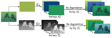
Figure 4. Generating various re-degraded underwater images.

3.2. Physical Knowledge-guided Dynamic Network

In this part, we introduce the developed model in detail, as shown in Fig. 3. The proposed GUPDM mainly consists of three parts: atmosphere-based dynamic structure, transmission-guided dynamic structure and prior-based multi-scale structure. ADS and TDS use dynamic convolutions to adaptively extract prior information from underwater images and generate parameters for PMS. We combine the meta-learning strategy to train our physical knowledge-based networks. This procedure can prompt our GUPDM to attend to different water types. Thus, the whole network can adaptively select appropriate parameters according to the water types of input images, achieving more robustness and generalization capacity.

Atmosphere-guided Dynamic Structure. With the degraded underwater model in Eq. (1), this work varies the atmosphere light $\mathbf{A}_{c}$ to different values, i.e., $\mathbf{A}_{c}^{m},\ m=1,\cdots,M$, obtaining $M$ degraded underwater types:

$$\mathbf{I}_{c}^{m}=\mathcal{G}_{\mathbf{A}}(\mathbf{A}_{c})=\lambda_{c}^{m}\mathbf{A}_{c}.$$

where $c\in\{r,g,b\}$ and $\lambda_{c}^{m}\in(0.3,0.6)$ is randomly generated degradation level. Then, to adaptively extract atmosphere-based prior information, we design ADS (i.e., $\mathcal{A}(\bm{\theta})$) with dynamic convolutions. We formulate this procedure as:

$$\mathbf{f}_{\text{ADS}}=\mathcal{A}(\bm{\theta},\mathbf{A}_{c}^{m};\{\mathbf{I}_{c}^{m}\}),\ m=1,\cdots,M.$$

The ADS consists of duplicated blocks composed of two Dynamic Convolutions (DC) (Chen et al., 2020) and one Global Average Pooling (GAP) module. The schematic of DC is depicted in Fig.3 where DC aggregates multiple parallel convolution kernels dynamically based upon their attentions, boosting the model complexity without increasing the network depth or width.

Algorithm 1 GUPDM Updating Framework

0:  Paired underwater data, necessary initialization parameters.

1:  $t=1$;

2:  while Not Converge do

3:     Use a batch of images $\mathbf{I}_{c}(x)$ as input :

4:     $\widetilde{\mathbf{J}}_{c}(x)\leftarrow\mathcal{N}(\bm{\omega};\mathcal{A}(\bm{\theta},\mathbf{A}_{c}),\mathcal{T}(\bm{\phi},\mathbf{T}_{c});\mathbf{I}_{c}(x))$

5:     Evaluate the total loss in $L_{\text{total}}=L(\widehat{\mathbf{J}},\mathbf{I}_{\text{gt}};\mathbf{I}_{c}(x))$

6:     $\#$ Update the parameters $\bm{\omega}$ of PMS

7:     $\bm{\omega}\leftarrow\bm{\omega}-\rho_{0}\nabla_{\bm{\omega}}L_{\text{total}}$

8:     if $(t\ Mod\ t_{0})=0$ then

9:        Generating $M$ patches degraded underwater images by $\mathcal{G}_{\mathbf{A}}$ as input $\mathbf{I}_{c}^{m}(x)$:

10:        $\widehat{\mathbf{J}}_{c}(x)\leftarrow\mathcal{N}(\bm{\omega};\mathcal{A}(\bm{\theta},\mathbf{A}_{c}^{m}),\mathcal{T}(\bm{\phi},\mathbf{T}_{c}(x);\mathbf{I}_{c}(x))$

11:        Evaluate the total loss in

12:        $L_{\text{total}}^{A}=\sum_{m=1}^{M}L(\widehat{\mathbf{J}},\mathbf{I}_{\text{gt}};\mathbf{I}_{c}^{m}(x),\mathbf{I}_{c}(x))$

13:        $\#$ Update the parameters $\bm{\theta}$ of ADS

14:        $\bm{\theta}\leftarrow\bm{\theta}-\rho_{1}\nabla_{\bm{\theta}}L_{\text{total}}^{A}$

15:     end if

16:     if $(t\ Mod\ t_{1})=0$ then

17:        Generating $N$ patches degraded underwater images by $\mathcal{G}_{\mathbf{T}}$ as input $\mathbf{I}_{c}^{n}(x)$:

18:        $\bar{\mathbf{J}}_{c}(x)\leftarrow\mathcal{N}(\bm{\omega};\mathcal{A}(\bm{\theta},\mathbf{A}_{c}^{m}),\mathcal{T}(\bm{\phi},\mathbf{T}_{c}^{n}(x);\mathbf{I}_{c}(x))$

19:        Evaluate the total loss in

20:        $L_{\text{total}}^{T}=\sum_{n=1}^{N}L(\bar{\mathbf{J}},\mathbf{I}_{\text{gt}};\mathbf{I}_{c}^{n}(x),\mathbf{I}_{c}(x))$

21:        $\#$ Update the parameters $\bm{\phi}$ of TDS

22:        $\bm{\phi}\leftarrow\bm{\phi}-\rho_{2}\nabla_{\bm{\phi}}L_{\text{total}}^{T}$

23:     end if

24:     $t=t+1$

25:  end while

Transmission-guided Dynamic Structure. We first estimate the transmission map $\mathbf{T}_{c}(x)$ via general dark channel prior (UDCP (Drews et al., 2013)). Since the transmission $\mathbf{T}_{c}(x)$ can reflect water types, we vary it through multiplying $\mathbf{T}_{c}(x)$ with randomly generated coefficients:

$$\mathbf{T}_{c}^{n}(x)=\mathcal{G}_{\mathbf{T}}(\mathbf{T}_{c}(x))=\gamma_{c}^{n}\cdot\mathbf{T}_{c}(x),n=1,\cdots,N,$$

where $\gamma_{c}^{n}\in(0.5,1.1)$ is the random coefficient. We then introduce a TDS (i.e., $\mathcal{T}(\bm{\phi})$) to enable our model to adaptively select appropriate parameters according to water types while paying more attention to various image details. We formulate this step as:

$$\mathbf{f}_{\text{TDS}}=\mathcal{T}(\bm{\phi},\mathbf{T}_{c}^{n};\{\mathbf{I}_{c}^{n}\}),\ n=1,\cdots,N.$$

Specifically, $\mathbf{f}_{\text{TDS}}$ and the transmission map $\mathbf{f}_{\text{m}}$ are integrated in Transmission Guided Feature Extraction module $\mathcal{M}$ (i.e., TGFE). The TDS has the same base structure with ADS.

Table 1. Quantitative comparisons on datasets with reference. We employ experiment on four datasets and three metrics, and achieve the best performance under most settings. We highlight the best result in black bold and underline the second ones.

Datasets	Metrics	UDCP (Drews et al., 2013)	Fusion (Ancuti et al., 2012)	Water-Net (Li et al., 2019a)	UGAN (Fabbri et al., 2018)	FUnIEGAN (Islam et al., 2020b)	Ucolor (Li et al., 2021)	USUIR (Fu et al., 2022a)	PUIE_net (Fu et al., 2022b)	Uranker-NU2Net (Guo et al., 2022)	Semi-UIR (Huang et al., 2023)	Ours
	PSNR$\uparrow$	16.38	17.61	20.14	21.89	18.43	22.23	18.2	17.7	23.92	18.7	25.48
Test-E515	SSIM$\uparrow$	0.64	0.75	0.68	0.8	0.76	0.83	0.74	0.76	0.84	0.73	0.86
	MSE$\downarrow$	1990	1331	826	556	1115	492	1153	1424	368	1015	254
	PSNR$\uparrow$	13.05	17.6	19.11	20.51	16.81	15.52	20.64	19.21	20.47	22.42	21.53
Test-U90	SSIM$\uparrow$	0.62	0.77	0.79	0.79	0.74	0.67	0.85	0.87	0.85	0.89	0.86
	MSE$\downarrow$	3779	1331	1220	911	1778	2217	716	966	879	522	721
	PSNR$\uparrow$	12.66	14.48	17.73	24.43	19.43	17.92	19.35	19.61	24.66	22.36	25.36
Test-L504	SSIM$\uparrow$	0.62	0.79	0.82	0.86	0.81	0.75	0.85	0.86	0.92	0.86	0.93
	MSE$\downarrow$	4529	3501	1361	285	891	1596	933	840	296	522	261
	PSNR$\uparrow$	18.26	14.58	22.46	21.93	18.35	21.79	17.87	17.09	23.09	18.68	24.34
Test-U120	SSIM$\uparrow$	0.72	0.54	0.79	0.77	0.73	0.76	0.72	0.72	0.77	0.72	0.79
	MSE$\downarrow$	1249	2968	458	525	1172	495	1222	1633	370	1005	297

Table 2. Averaged unsupervised scores (i.e., PS, UIQM, UCIQE, NIQE and URanker) on three real-world underwater datasets without reference images (i.e., Test-C60, Test-R300 and Test-S16).

Datasets	Test-C60					Test-R300					Test-S16
	PS$\uparrow$	UIQM$\downarrow$	UCIQE$\uparrow$	NIQE$\downarrow$	Uranker $\uparrow$	PS$\uparrow$	UIQM$\downarrow$	UCIQE$\uparrow$	NIQE$\downarrow$	Uranker$\uparrow$	PS$\uparrow$	UIQM$\downarrow$	UCIQE$\uparrow$	NIQE$\downarrow$	Uranker$\uparrow$
Water-Net (Li et al., 2019a)	6.45	2.86	27.39	4.97	0.93	4.45	2.58	27.49	4.91	2.17	6.18	2.11	24.66	6.41	1.99
FUnIEGAN (Islam et al., 2020b)	4.58	4.54	30.05	6.21	1.67	4.22	4.00	28.58	4.89	2.25	6.51	3.27	27.81	6.49	2.02
USUIR (Fu et al., 2022a)	3.94	4.71	32.04	5.74	1.14	3.66	3.34	20.34	4.68	1.83	5.31	3.30	28.24	6.37	0.42
Fusion (Ancuti et al., 2012)	4.73	2.67	32.26	5.29	1.24	3.18	3.06	31.58	4.36	2.34	7.86	2.01	31.35	12.19	0.91
Ucolor (Li et al., 2021)	6.26	4.31	24.27	5.34	0.63	4.40	3.36	20.48	4.83	0.77	8.90	3.11	27.51	11.85	0.58
UDCP (Drews et al., 2013)	6.66	1.54	32.55	5.44	0.62	4.88	2.30	28.72	5.41	0.46	7.47	1.02	33.92	9.05	0.26
UGAN (Fabbri et al., 2018)	4.53	4.69	31.08	6.81	1.91	4.03	4.29	29.44	5.22	2.61	6.01	3.29	28.26	6.98	2.02
PUIE_NET (Fu et al., 2022b)	4.54	3.64	27.25	6.22	1.05	4.27	4.00	26.83	4.90	1.77	6.99	3.34	27.81	7.97	0.99
Uranker-NU2Net (Guo et al., 2022)	4.26	4.57	28.90	5.79	1.18	4.65	4.18	28.63	4.69	2.30	5.84	3.26	30.17	6.66	2.11
Semi-UIR (Huang et al., 2023)	3.97	4.74	30.63	5.77	1.69	4.52	4.11	29.23	4.52	2.45	5.79	2.63	30.00	6.43	1.98
Ours	6.45	4.88	32.36	4.76	1.94	4.95	4.35	31.05	4.26	2.64	8.06	3.52	31.78	6.18	2.22

Prior-based Multi-scale Structure. This structure is a basic part of our underwater image enhancement. First, to mine the physical knowledge and features of depth-texture information at different scales, we adopt the prior-based multi-scale structure to estimate the preliminary pixel feature $\mathbf{f}_{\text{PMS}}$ in this branch.

$$\mathbf{J}_{c}(x)\leftarrow\mathcal{N}(\bm{\omega};\mathcal{A}(\bm{\theta},\mathbf{A}_{c}),\mathcal{T}(\bm{\phi},\mathbf{T}_{c});\mathbf{I}_{c}(x)).$$

As for $\mathcal{N}$, it mainly consists of a series of HMH and 3H modules with a tailored Transmission-Guided Feature Extraction (TGFE) module at its bottleneck. HMH comprises a Hyper Residual Block (HRB), a Multi-scale Feature Extraction module (MFE) and another HRB, while 3H consists of three HRBs. The HRB converts input parameters (i.e. $\mathbf{f}_{\text{ADS}}$ or $\mathbf{f}_{\text{TDS}}$) to weights of convolution block via a Fully Connected (FC) layers. The detailed structure of the MFE module is shown in top right of Fig. 3. To improve the receptive field of the framework, we utilize three convolution blocks with different kernel sizes $1\times 1$, $3\times 3$ and $5\times 5$, generating three feature maps. We then employ global max pooling and average pooling in channel attention block to automatically extract and fuse the main features from three feature maps at different scales. TGFE consists of a HRB, a TC, a MFE and another HRB sequentially, integrating the transmission feature $\mathbf{f}_{m}$ to tackle the blur and haze.

3.3. Loss Functions and Training Procedure

We carefully design the training loss functions to guide the model to produce enhanced results with minimum color artifacts, blurriness and the closest details to reference images. Firstly, we use pretrained VGG16 network to extract the feature in $3^{th},8^{th}$ and $15^{th}$ layers to formulate the perceptional loss $L_{per}$:

(3) $$L_{\text{per}}(\mathbf{J},\mathbf{I}_{\text{gt}})=L_{\text{MSE }}\left(\operatorname{VGG}_{3,8,15}(\mathbf{J}),\mathrm{VGG}_{3,8,15}\left(\mathbf{I}_{\text{gt}}\right)\right),$$

where $L_{\text{MSE }}$ denotes the Mean Square Error (MSE). We also impose the smooth $L_{1}-\operatorname{loss}$ as reconstruction loss since we notice that unnecessary interference often occurs from the background color:

(4) $$L_{1}(\mathbf{J},\mathbf{I}_{\text{gt}})=\frac{1}{n}\sum_{i=1}^{n}|\mathbf{J}(i)-\mathbf{I}_{\text{gt}}(i)|,$$

where $n=H\times W$ is the overall pixel number. We furthermore apply the SSIM loss to focus more on the structural details. Thus, the total loss function can be summarized as follows:

(5) $$L(\mathbf{J},\mathbf{I}_{\text{gt}})=\ell_{1}+\lambda_{1}\mathcal{L}_{\text{SSIM }}+\lambda_{2}\mathcal{L}_{\text{per }}$$

where $\lambda_{1}$ and $\lambda_{2}$ stand for the weights of each loss functions.

We illustrate the training procedure of proposed method in Algorithm  1. In particular, we first train the base-net PMS with given atmosphere $\mathbf{A}_{c}$ and transmission $\mathbf{T}_{c}$ and loss function $L(\widetilde{\mathbf{J}},\mathbf{I}_{\text{gt}};\mathbf{I}_{c}(x))$. Next, we fix the base-net PMS and update parameter of ADS (i.e., $\bm{\theta}$) which is optimized with loss $L(\widehat{\mathbf{J}},\mathbf{I}_{\text{gt}};\mathbf{I}_{c}^{m}(x),\mathbf{I}_{c}(x))$. Similarly, the parameter of TDS (i.e., $\bm{\phi}$ ) is updated through optimizing $L(\bar{\mathbf{J}},\mathbf{I}_{\text{gt}};\mathbf{I}_{c}^{n}(x),\mathbf{I}_{c}(x))$. The ADS, TDS and PMS are trained in an alternate manner until they converge.

4. Experimental Results

This section first introduces the implementation details in Subsection 4.1. Then, to evaluate the performance when comparing with existing state-of-the-art approaches, a series of qualitative and quantitative assessments are conducted in Subsection 4.2. To analyze the developed method, we conduct various ablation studies to verify the effectiveness of different branches in Subsection 4.3. More experimental results are provided in our supplementary material.

4.1. Implantation Details

Datasets. Our model is trained on LSUI (Peng et al., 2023), a real underwater dataset, which consisting 4500 training pairs and 504 test pairs (i.e. Test-504). In order to evaluate the effectiveness and robustness of our proposed method, we test it on six real world datasets: Test-U90 (i.e. UIEB (Li et al., 2019a)), Test-L504 (i.e. LSUI (Peng et al., 2023)), Test-U120 (i.e. UFO (Islam et al., 2020a)), Test-S16 (i.e. SQUID (Berman et al., 2020)), Test-R300 (i.e. RUIE (Liu et al., 2020a)) and Test-C60 (Li et al., 2019a), and a synthetic one: Test-E515 (i.e. EUVP (Islam et al., 2020c)). There are two categories of testing datasets: those that have reference images (either real or generated by another method) and those that don’t. The first type includes Test-E515, Test-U90, Test-L504 and Test-U120 datasets, where Test-E515 uses synthetic images created by a CycleGAN-based model. The second type includes Test-C60, Test-R300 and Test-S16 datasets. Specifically, Test-C60 contains 60 difficult images from UIEB and Test-S16 has 16 images from its original dataset without references.

EUVP
UIEB
LSUI
UFO
	FUnIEGAN	USUIR	Ucolor	PUIENet	Uranker-NU2Net	Semi-UIR	Ours	Reference

Figure 5. Visual comparison with different methods on synthesis dataset (EUVP) and real-world datasets (UIEB, LSUI and UFO). Comparing with FUnIEGAN, USUIR, Ucolor, PUIENet, URanker, Semi-UIR, our developed method (i.e., SIM-Net) achieves an natural color and preserves more details, performing the best visual quality.

Test-C60
Test-R300
Test-S16
	Input	FUnIEGAN	USUIR	Ucolor	PUIENet	Uranker-NU2Net	Semi-UIR	Ours

Figure 6. Visual comparison on datasets with no references (Test-C60, Test-R300, Test-S16) with Uranker metric value annotated. Comparing with FUnIEGAN, USUIR, Ucolor, PUIENet, URanker, Semi-UIR, our developed method performs the best visual quality.

Settings. PyTorch is utilized to implement proposed network and we use NVIDIA RTX 3090 cards to perform all the experiments. We use Adam as optimizer while training all the models we compare. All the images are resized to $256\times 256$. During the training process, we set the total epoch to 200, the batchsize to 8 and the initial learning rate of PMS, ADS and TDS are 1e-4, 1e-4 and 1e-6. Moreover, in Algorithm 1 the update step $t_{0}$ is 10 and $t_{1}$ is 11. The coefficientes $\lambda_{1},\lambda_{2}$ of Eq. 5 are 0.04 and 0.02.

Evaluation Metrics. We adopt both reference-dependent and non-reference evaluation measurements to comprehensively assess the performance of our model. For reference-dependent metrics, we select Peak Signal to Noise Ratio (PSNR), Structural Similarity (SSIM) and Mean Square Error (MSE). As for the non-reference metrics, we employ Underwater Color Image Quality Evaluation (UCIQE (Yang and Sowmya, 2015)), Underwater Image Quality Measure (UIQM (Panetta et al., 2015)) and Perceptual Scores (PS) which reflect the visual quality of the image from a human perspective. We also adopt Natural Image Quality Evaluator (NIQE (Mittal et al., 2012)), which evaluates the naturalness of generated images. Furthermore, we utilize URanker (Guo et al., 2022), an UIQA method based on the Transformer. We apply these metrics on real-world underwater challenge datasets.

4.2. Comparing with Other UIE Methods

In this section, we make comparisons with traditional methods (i.e., Fusion (Ancuti et al., 2012) and UDCP (Drews et al., 2013) ), GAN-based methods (i.e., UGAN (Fabbri et al., 2018), FUnIEGAN (Islam et al., 2020b)) and CNN-based approaches (i.e, Water-Net (Li et al., 2019a), Ucolor (Li et al., 2021), USUIR (Fu et al., 2022a), PUIE_net (Fu et al., 2022b), Uranker-NU²Net (Guo et al., 2022) and Semi-UIR (Huang et al., 2023)). All of the competitive models are retrained with their public codes on LSUI dataset for fair comparison.

Quantitative Comparisons. We first evaluate the capacity of our method quantitatively and summarize the comparisons results in Tab. 1 and Tab. 2 where the best result is highlighted in black bold and the second one is marked underline. From Tab. 1, we can observe that, our proposed method ranks the first in Test-E515, Test-L504 and Test-U120 datasets in all three metrics. We achieve the percentage gain of 6.5%, 2.8% and 5.4% regarding PSNR and obtain leading 30.9%, 8.4% and 19.7% percentage improvement regarding MSE metric in three datasets, respectively, indicating our results are more consistent with ground-truth images and our superior performance compared to other methods. Besides, we are only slightly behind Semi-UIR in Test-U90 dataset, with a minor gap. Moreover, Tab. 2 demonstrates that we can achieve the best result in UIQM, NIQE and Uranker metrics, and gain the second performance in all other evaluation cases. These indicate that our method is equipped with superior performance when compared to other methods on challenge dataset using unsupervised metrics.

Qualitative Comparisons. We display the results on synthesized datasets in Fig. 5 and the images from datasets with no references in Fig. 6 where we manually pick one picture from each dataset. Besides, we annotate the corresponding PSNR, MSE results of each image in the right bottom in Fig. 5 and the Uranker metric in Fig. 6. In general, our method provides images with more natural color, abundant details, and less blurs. We have the closest overall chroma to references and the best metrics as in all four rows in Fig. 5. In Fig. 6, FGAN, USUIR, Ucolor and PUIENet fail to predict the plausible color, suffering from over or under enhancement results. Uranker-NU²Net and Semi-UIR achieve good performance but obtain lower value of Uranker metric as depicted in the right bottom. Our method attains the best results both visually and metrically.

Input	w/o ADS	w/o TDS	w/ ADS, w/o $\mathcal{G}_{\mathbf{A}}$	w/ TDS, w/o $\mathcal{G}_{\mathbf{T}}$	Ours	Reference

Figure 7. Visual results of ablation on ADS, TDS, $\mathcal{G}_{\mathbf{A}}$ and $\mathcal{G}_{\mathbf{T}}$. The second row show the corresponding heat feature map.

Input	w/o 3H	w/o HMH	Ours

Figure 8. Ablation study on 3H and HMH module. We show the corresponding histogram distance between enhanced images and references images in the second row.

Table 3. Analyzing the effectiveness of ADS, TDS, $\mathcal{G}_{\mathbf{A}}$ and $\mathcal{G}_{\mathbf{T}}$.

Baselines	PSNR$\uparrow$	SSIM$\uparrow$	MSE$\downarrow$
w/o ADS	0.84	19.90	912
w/o TDS	0.85	20.67	789
w/ ADS, w/o $\mathcal{G}_{\mathbf{A}}$	0.85	20.69	774
w/ TDS, w/o $\mathcal{G}_{\mathbf{T}}$	0.84	20.30	830
Ours	0.86	21.53	721

Table 4. Analyzing the effectiveness of different Modules (including TGFE, 3H and HMH) on UIEB dataset.

Modules	Ablation	Metrics
		PSNR$\uparrow$	SSIM$\uparrow$	MSE$\downarrow$
TGFE	w/o TGFE	19.82	0.83	941
	w/o TC	21.01	0.85	745
	w/o MFE	20.86	0.85	780
	w/o HRB	20.92	0.85	727
3H	w/o 3H	20.86	0.85	764
HMH	w/o HMH	18.41	0.78	1143
Ours	-	21.53	0.86	721

Table 5. Analyzing the effectiveness of $\mathbf{f}_{\text{ADS}}$ and $\mathbf{f}_{\text{TDS}}$.

Modules	Baselines	Average Metrics
		PSNR$\uparrow$	SSIM$\uparrow$	MSE$\downarrow$
3H	w/o $\mathbf{f}_{\text{ADS}}$	0.85	23.87	404
HMH	w/o $\mathbf{f}_{\text{ADS}}$	0.85	23.85	411
TGFE	w/o $\mathbf{f}_{\text{TDS}}$	0.84	23.65	427
Full Model	w/o $\mathbf{f}_{\text{ADS}}$, w/o $\mathbf{f}_{\text{TDS}}$	0.84	22.99	491
	w/ $\mathbf{f}_{\text{ADS}}$, w/ $\mathbf{f}_{\text{TDS}}$	0.86	24.17	383

Table 6. Analyzing the effectiveness of training schema.

Baselines	PSNR$\uparrow$	SSIM$\uparrow$	MSE$\downarrow$
(a) end-to-end	0.84	20.09	901
(b) ADS and TDS together	0.85	20.95	726
(c) ADS, TDS and PMS together	0.85	20.89	743
(d) ADS, TDS and PMS separate	0.86	21.53	721

4.3. Ablation Study

Analysis the effectiveness of ADS and TDS. We investigate the effectiveness of physical knowledge-based dynamic structure (i.e., ADS and TDS). We show the statistical results in Tab. 3 and visual images in Fig. 7. Without the whole ADS branch, the model cannot capture the atmosphere information. Without TDS branch providing ample transmission information, the performance of our model also deteriorates, resulting in less vivid images. Besides, ablating $\mathcal{G}_{\mathbf{A}}$ and $\mathcal{G}_{\mathbf{T}}$ that generates various degraded priors deprives the model from learning diverse atmosphere and transmission scenarios in ADS and TDS, respectively. Thus the produced images lack detail as shown in the body of fish in the heat map in second row of Fig. 7.

Analysis the components of PMS. To verify how each module in our method plays a irreplaceable role, we ablate: the Transmission-map Guided Feature Extraction (TGFE), 3H and HMH. Furthermore, we exam the Transmission-based Connection (TC) block, Multi-scale Feature extraction (MFE) module and Hyper Residual Block (HRB) in TGFE to dig the effectiveness of each module. Note that when ablating the 3H and HMH module, we change all four modules posed in PMS. The corresponding results are listed in Tab. 4.

Without MFE module extracting multiple feature from distinct scales, the performance of our model decreases which is reflected in reported scores. 3H module, consisting of three hyper residual block, obtains weights from dynamic prior hyper net and serves as a color optimizer. Thus removing them leads to suboptimal scores. Furthermore, we display the visual results in Fig. 8 which demonstrates that, without 3H and HMH integrating prior knowledge, the generated images are more blur and dull, the histogram distance to references is also worsen.

Influence of $\mathbf{f}_{\text{ADS}}$ and $\mathbf{f}_{\text{TDS}}$ to generalization capacity. We discuss the impact of $\mathbf{f}_{\text{ADS}}$ and $\mathbf{f}_{\text{TDS}}$ here. Note that removing them means that the weights of res-blocks in each setting are directly learned form training phrase, not obtained from hyper-nets. We perform experiments on res-blocks in 3H, HMH and TGFE. All ablations are conducted on LSUI dataset for training and evaluated on four datasets: Test-E515, Test-U90, Test-L504 and Test-U120. We compute the average scores regarding the PSNR, SSIM and MSE metrics on four datasets and report them in Tab. 5.

We observe that, the full model ranks the first in all three measurements, indicating that we achieve the best generalization ability among datasets. Without $\mathbf{f}_{\text{ADS}}$ or $\mathbf{f}_{\text{TDS}}$ in any position, the performance deteriorates. Therefore, we keep $\mathbf{f}_{\text{ADS}}$ and $\mathbf{f}_{\text{TDS}}$ in those modules to ensure a better generalization capability.

Analysis on training strategy. We list different training methods and their results in Tab.  6. Specifically, (a) means that we train two hypernets and PMS in an end-to-end manner. (b) means that we optimize ADS and TDS together, and then optimize PMS alternately. (c) means that we optimize three networks (ADS, TDS and PMS) all together. (d) is our strategy which separately optimizes three networks. It can be seen that the our training strategy is of great important. We argue that this can be attributed to the inconsistent convergence speed of the hyper-nets and the main net. Thus, we train and optimize three nets in an alternate and separate way.

5. Conclusion

In this work we developed a novel approach named GUPDM for underwater image enhancement. We tailored ADS and TDS as hyper-nets to generate parameters for PMS via varied global atmosphere and transmission to cover complex underwater scenes. Experimental results illustrated our superior performance in terms of quantitative scores, visual results and generalization ability.

- (1)
- Akkaynak and Treibitz (2018) Derya Akkaynak and Tali Treibitz. 2018. A revised underwater image formation model. In Proceedings of the IEEE conference on Computer Vision and Pattern Recognition. 6723–6732.
- Akkaynak and Treibitz (2019a) Derya Akkaynak and Tali Treibitz. 2019a. Sea-thru: A method for removing water from underwater images. In Proceedings of the IEEE/CVF conference on Computer Vision and Pattern Recognition. 1682–1691.
- Akkaynak and Treibitz (2019b) Derya Akkaynak and Tali Treibitz. 2019b. Sea-thru: A method for removing water from underwater images. In Proceedings of the IEEE/CVF conference on Computer Vision and Pattern Recognition. 1682–1691.
- Ancuti et al. (2012) Cosmin Ancuti, Codruta Orniana Ancuti, Tom Haber, and Philippe Bekaert. 2012. Enhancing underwater images and videos by fusion. In 2012 IEEE conference on Computer Vision and Pattern Recognition. IEEE, 81–88.
- Ancuti et al. (2019) Codruta O Ancuti, Cosmin Ancuti, Christophe De Vleeschouwer, and Mateu Sbert. 2019. Color channel compensation (3C): A fundamental pre-processing step for image enhancement. IEEE Transactions on Image Processing 29 (2019), 2653–2665.
- Berman et al. (2020) Dana Berman, Deborah Levy, Shai Avidan, and Tali Treibitz. 2020. Underwater single image color restoration using haze-lines and a new quantitative dataset. IEEE Transactions on Pattern Analysis and Machine Intelligence 43, 8 (2020), 2822–2837.
- Buchsbaum (1980) Gershon Buchsbaum. 1980. A spatial processor model for object colour perception. Journal of the Franklin institute 310, 1 (1980), 1–26.
- Chen et al. (2020) Yinpeng Chen, Xiyang Dai, Mengchen Liu, Dongdong Chen, Lu Yuan, and Zicheng Liu. 2020. Dynamic convolution: Attention over convolution kernels. In Proceedings of the IEEE/CVF conference on Computer Vision and Pattern Recognition. 11030–11039.
- Chiang and Chen (2011) John Y Chiang and Ying-Ching Chen. 2011. Underwater image enhancement by wavelength compensation and dehazing. , 1756–1769 pages.
- Drews et al. (2013) Paul Drews, Erickson Nascimento, Filipe Moraes, Silvia Botelho, and Mario Campos. 2013. Transmission estimation in underwater single images. In Proceedings of the IEEE international conference on computer vision workshops. 825–830.
- Fabbri et al. (2018) Cameron Fabbri, Md Jahidul Islam, and Junaed Sattar. 2018. Enhancing Underwater Imagery Using Generative Adversarial Networks. In 2018 IEEE International Conference on Robotics and Automation (ICRA). 7159–7165. https://doi.org/10.1109/ICRA.2018.8460552
- Fu et al. (2022a) Zhenqi Fu, Huangxing Lin, Yan Yang, Shu Chai, Liyan Sun, Yue Huang, and Xinghao Ding. 2022a. Unsupervised Underwater Image Restoration: From a Homology Perspective. In Proceedings of the AAAI Conference on Artificial Intelligence. 643–651.
- Fu et al. (2022b) Zhenqi Fu, Wu Wang, Yue Huang, Xinghao Ding, and Kai-Kuang Ma. 2022b. Uncertainty Inspired Underwater Image Enhancement. In Computer Vision–ECCV 2022: 17th European Conference, Tel Aviv, Israel, October 23–27, 2022, Proceedings, Part XVIII. Springer, 465–482.
- Galdran et al. (2015) Adrian Galdran, David Pardo, Artzai Picón, and Aitor Alvarez-Gila. 2015. Automatic red-channel underwater image restoration. Journal of Visual Communication and Image Representation 26 (2015), 132–145.
- Ghani and Isa (2015) Ahmad Shahrizan Abdul Ghani and Nor Ashidi Mat Isa. 2015. Enhancement of low quality underwater image through integrated global and local contrast correction. Applied Soft Computing 37 (2015), 332–344.
- Guo et al. (2022) Chunle Guo, Ruiqi Wu, Xin Jin, Linghao Han, Zhi Chai, Weidong Zhang, and Chongyi Li. 2022. Underwater ranker: learn which is better and how to be better. arXiv preprint arXiv:2208.06857 (2022).
- Guo et al. (2019) Yecai Guo, Hanyu Li, and Peixian Zhuang. 2019. Underwater image enhancement using a multiscale dense generative adversarial network. IEEE Journal of Oceanic Engineering 45, 3 (2019), 862–870.
- Ha et al. (2016) David Ha, Andrew Dai, and Quoc V Le. 2016. Hypernetworks. arXiv preprint arXiv:1609.09106 (2016).
- Huang et al. (2023) Shirui Huang, Keyan Wang, Huan Liu, Jun Chen, and Yunsong Li. 2023. Contrastive Semi-supervised Learning for Underwater Image Restoration via Reliable Bank. arXiv preprint arXiv:2303.09101 (2023).
- Iqbal et al. (2010) Kashif Iqbal, Michael Odetayo, Anne James, Rosalina Abdul Salam, and Abdullah Zawawi Hj Talib. 2010. Enhancing the low quality images using unsupervised colour correction method. In 2010 IEEE International Conference on Systems, Man and Cybernetics. IEEE, 1703–1709.
- Islam et al. (2020a) Md Jahidul Islam, Peigen Luo, and Junaed Sattar. 2020a. Simultaneous enhancement and super-resolution of underwater imagery for improved visual perception. arXiv preprint arXiv:2002.01155 (2020).
- Islam et al. (2020b) Md Jahidul Islam, Youya Xia, and Junaed Sattar. 2020b. Fast Underwater Image Enhancement for Improved Visual Perception. IEEE Robotics and Automation Letters 5, 2 (2020), 3227–3234.
- Islam et al. (2020c) Md Jahidul Islam, Youya Xia, and Junaed Sattar. 2020c. Fast underwater image enhancement for improved visual perception. IEEE Robotics and Automation Letters 5, 2 (2020), 3227–3234.
- Jiang et al. (2022a) Zhiying Jiang, Zhuoxiao Li, Shuzhou Yang, Xin Fan, and Risheng Liu. 2022a. Target Oriented Perceptual Adversarial Fusion Network for Underwater Image Enhancement. IEEE Transactions on Circuits and Systems for Video Technology (2022).
- Jiang et al. (2022b) Zhiying Jiang, Zengxi Zhang, Yiyao Yu, and Risheng Liu. 2022b. Bilevel modeling investigated generative adversarial framework for image restoration. The Visual Computer (2022), 1–13.
- Land (1977) Edwin H Land. 1977. The retinex theory of color vision. Scientific american 237, 6 (1977), 108–129.
- Li et al. (2021) Chongyi Li, Saeed Anwar, Junhui Hou, Runmin Cong, Chunle Guo, and Wenqi Ren. 2021. Underwater image enhancement via medium transmission-guided multi-color space embedding. IEEE Transactions on Image Processing 30 (2021), 4985–5000.
- Li et al. (2020) Chongyi Li, Saeed Anwar, and Fatih Porikli. 2020. Underwater scene prior inspired deep underwater image and video enhancement. Pattern Recognition 98 (2020), 107038.
- Li et al. (2019a) Chongyi Li, Chunle Guo, Wenqi Ren, Runmin Cong, Junhui Hou, Sam Kwong, and Dacheng Tao. 2019a. An underwater image enhancement benchmark dataset and beyond. IEEE Transactions on Image Processing 29 (2019), 4376–4389.
- Li et al. (2016) Chong-Yi Li, Ji-Chang Guo, Run-Min Cong, Yan-Wei Pang, and Bo Wang. 2016. Underwater image enhancement by dehazing with minimum information loss and histogram distribution prior. IEEE Transactions on Image Processing 25, 12 (2016), 5664–5677.
- Li et al. (2019b) Hanyu Li, Jingjing Li, and Wei Wang. 2019b. A fusion adversarial underwater image enhancement network with a public test dataset. arXiv preprint arXiv:1906.06819 (2019).
- Lin et al. (2021) Runjia Lin, Jinyuan Liu, Risheng Liu, and Xin Fan. 2021. Global structure-guided learning framework for underwater image enhancement. The Visual Computer (2021), 1–16.
- Lin et al. (2020) Xi Lin, Zhiyuan Yang, Qingfu Zhang, and Sam Kwong. 2020. Controllable pareto multi-task learning. arXiv preprint arXiv:2010.06313 (2020).
- Liu et al. (2018) Risheng Liu, Xin Fan, Minjun Hou, Zhiying Jiang, Zhongxuan Luo, and Lei Zhang. 2018. Learning aggregated transmission propagation networks for haze removal and beyond. IEEE transactions on neural networks and learning systems 30, 10 (2018), 2973–2986.
- Liu et al. (2020a) Risheng Liu, Xin Fan, Ming Zhu, Minjun Hou, and Zhongxuan Luo. 2020a. Real-world underwater enhancement: Challenges, benchmarks, and solutions under natural light. IEEE Transactions on Circuits and Systems for Video Technology 30, 12 (2020), 4861–4875.
- Liu et al. (2019) Risheng Liu, Minjun Hou, Jinyuan Liu, Xin Fan, and Zhongxuan Luo. 2019. Compounded layer-prior unrolling: A unified transmission-based image enhancement framework. In 2019 IEEE International Conference on Multimedia and Expo (ICME). IEEE, 538–543.
- Liu et al. (2022a) Risheng Liu, Zhiying Jiang, Shuzhou Yang, and Xin Fan. 2022a. Twin adversarial contrastive learning for underwater image enhancement and beyond. IEEE Transactions on Image Processing 31 (2022), 4922–4936.
- Liu et al. (2020b) Risheng Liu, Pan Mu, Xiaoming Yuan, Shangzhi Zeng, and Jin Zhang. 2020b. A generic first-order algorithmic framework for bi-level programming beyond lower-level singleton. In International Conference on Machine Learning. PMLR, 6305–6315.
- Liu et al. (2022b) Risheng Liu, Pan Mu, Xiaoming Yuan, Shangzhi Zeng, and Jin Zhang. 2022b. A general descent aggregation framework for gradient-based bi-level optimization. IEEE Transactions on Pattern Analysis and Machine Intelligence 45, 1 (2022), 38–57.
- Liu et al. (1995) Yung-Cheng Liu, Wen-Hsin Chan, and Ye-Quang Chen. 1995. Automatic white balance for digital still camera. IEEE Transactions on Consumer Electronics 41, 3 (1995), 460–466.
- Mittal et al. (2012) Anish Mittal, Rajiv Soundararajan, and Alan C Bovik. 2012. Making a “completely blind” image quality analyzer. IEEE Signal processing letters 20, 3 (2012), 209–212.
- Mu et al. (2022) Pan Mu, Haotian Qian, and Cong Bai. 2022. Structure-Inferred Bi-level Model for Underwater Image Enhancement. Proceedings of the 30th ACM International Conference on Multimedia (MM) (2022).
- Panetta et al. (2015) Karen Panetta, Chen Gao, and Sos Agaian. 2015. Human-visual-system-inspired underwater image quality measures. IEEE Journal of Oceanic Engineering 41, 3 (2015), 541–551.
- Peng et al. (2023) Lintao Peng, Chunli Zhu, and Liheng Bian. 2023. U-shape transformer for underwater image enhancement. In Computer Vision–ECCV 2022 Workshops: Tel Aviv, Israel, October 23–27, 2022, Proceedings, Part II. Springer, 290–307.
- Peng and Cosman (2017) Yan-Tsung Peng and Pamela C Cosman. 2017. Underwater image restoration based on image blurriness and light absorption. IEEE Transactions on Image Processing 26, 4 (2017), 1579–1594.
- Pizer (1990) Stephen M Pizer. 1990. Contrast-limited adaptive histogram equalization: Speed and effectiveness stephen m. pizer, r. eugene johnston, james p. ericksen, bonnie c. yankaskas, keith e. muller medical image display research group. In Proceedings of the first conference on visualization in biomedical computing, Atlanta, Georgia, Vol. 337. 1.
- Qian et al. (2022) Haotian Qian, Wentao Tong, Pan Mu, Zheyuan Liu, and Hanning Xu. 2022. Real-world Underwater Image Enhancement via Degradation-aware Dynamic Network. In PRICAI 2022: Trends in Artificial Intelligence: 19th Pacific Rim International Conference on Artificial Intelligence, PRICAI 2022, Shanghai, China, November 10–13, 2022, Proceedings, Part III. Springer, 530–541.
- Rahman et al. (1996) Zia-ur Rahman, Daniel J Jobson, and Glenn A Woodell. 1996. Multi-scale retinex for color image enhancement. In Proceedings of 3rd IEEE International Conference on Image Processing, Vol. 3. IEEE, 1003–1006.
- Wang et al. (2017) Yi Wang, Hui Liu, and Lap-Pui Chau. 2017. Single underwater image restoration using adaptive attenuation-curve prior. IEEE Transactions on Circuits and Systems I: Regular Papers 65, 3 (2017), 992–1002.
- Yang and Sowmya (2015) Miao Yang and Arcot Sowmya. 2015. An underwater color image quality evaluation metric. IEEE Transactions on Image Processing 24, 12 (2015), 6062–6071.
- Yin et al. (2022) Guanghao Yin, Wei Wang, Zehuan Yuan, Wei Ji, Dongdong Yu, Shouqian Sun, Tat-Seng Chua, and Changhu Wang. 2022. Conditional hyper-network for blind super-resolution with multiple degradations. IEEE Transactions on Image Processing 31 (2022), 3949–3960.
- Zhang et al. (2017) Shu Zhang, Ting Wang, Junyu Dong, and Hui Yu. 2017. Underwater image enhancement via extended multi-scale Retinex. Neurocomputing 245 (2017), 1–9.