Numerical Investigation of the Local Thermo-Chemical State in a Thermo-Acoustically Unstable Dual Swirl Gas Turbine Model Combustor

In this work, the thermo-acoustic instabilities of a gas turbine model combustor, the so-called SFB606 combustor, are numerically investigated using Large Eddy Simulation (LES) combined with tabulated chemistry and Artificial Thickened Flame (ATF) approach. The main focus is a detailed analysis of the thermo-acoustic cycle and the accompanied equivalence ratio oscillations and their associated convective time delay. In particular, the variations of the thermo-chemical state and flame characteristics over the thermo-acoustic cycle are investigated. For the operating point flame B ($P_{th}=25kW$, $\Phi=0.7$), the burner exhibits thermo-acoustic instabilities with a dominant frequency of $392\text{\,}\mathrm{Hz}\text{/}$, the acoustic eigenmode of the inner air inlet duct. These oscillations are accompanied by an equivalence ratio oscillation, which exhibits a convective time delay between the injection in the inner swirler and the flame zone. Two LES, one adiabatic and one accounting for heat losses at the walls by prescribing the wall temperatures from experimental data and Conjugated Heat Transfer (CHT) simulations, are conducted. Results with the enthalpy-dependent table are found to predict the time-averaged flow field in terms of velocity, major species, and temperature with higher accuracy than in the adiabatic case. Further, they indicate, that heat losses should be accounted for to correctly predict the flame position. Subsequently, the thermo-chemical state variations over the thermo-acoustic cycle for the enthalpy-dependant case are analyzed in detail and compared with experimental data in terms of phase-conditioned averaged profiles and conditional averages. An overall good prediction is observed, although an overestimation of the oscillation amplitude yields a slight over-prediction of the velocity field in the low-pressure phases. The results provide a detailed quantitative analysis of the thermo-acoustic feedback mechanism of this burner.

1 Introduction

To achieve high efficiency and low emission levels, modern gas turbines (GTs) are designed with swirl burners operating in the lean premixed or partially-premixed combustion regime [1, 2]. These burner configurations are, however, prone to hydrodynamic instabilities, such as Precessing Vortex Cores (PVC) [3, 1], and thermo-acoustic instabilities, that may affect the combustor operations and even damage GT components [4]. Multiple thermo-acoustic feedback loop mechanisms have been identified and discussed in several studies. Acoustic modes can induce oscillations on the flame front kinematics, which can lead to variations of the flame surface [5] and the flame positions [6] resulting in heat release rate oscillations. Thermo-acoustic modes can also be excited by vortex shedding as discussed in [7, 8]. Hydrodynamic instabilities and PVC may affect the thermo-acoustic cycle as well as the flame shape, as shown in [9, 10]. Furthermore, pressure oscillations in the air or fuel supply can yield equivalence ratio oscillations: they are convected into the flame zone causing heat release rate fluctuations [11, 12].

Although significant progress has been made in the understanding and prediction of combustion instabilities [2], accurately estimating their amplitude and frequency remains a challenge [4]. To enhance the understanding of combustion instabilities, gas turbine model combustors (GTMCs) have been intensively studied. Kim et al. [13] experimentally examined the response of a swirl-stabilized partially-premixed flame subjected to acoustic velocity and equivalence ratio oscillations. They found a dependency in the phase difference between the two perturbations determining the linear or non-linear flame response. Non-linear response in swirl stabilized flames are studied in [14] for various oscillation amplitudes and a flame transfer function model was developed to determine the limit cycle behavior. It was observed that a saturation of the equivalence ratio perturbation is achieved already at relatively small amplitudes due to the increased turbulent mixing. The DLR dual swirl burner [15, 16] and the PRECCINSTA burner [17, 12] are further examples of partially-premixed swirl GTMCs designed to investigate combustion instabilities, which have been used as benchmark configurations for numerical simulations and model development in numerous studies.

In the last decades, Large Eddy Simulations (LES) have become a fundamental resource for understanding complex three-dimensional turbulent reacting flows in combustors [18], both in stable and unstable regimes, see e.g. [19, 20, 21, 22, 23, 2]. Many of these studies applied simple kinetic mechanisms combined with the artificially thickened flame (ATF) approach [19, 20] or flamelet-based tabulated chemistry with ATF or presumed probability density function[24, 21, 22, 23]. Few studies were performed considering reduced finite-rate chemistry with the stochastic fields method as in [25]. One fundamental aspect in numerical simulations of GTs is the modeling of heat losses for both steady [26, 24, 27] and oscillating operating points [28, 29]. Major heat transfer phenomena include the heat transfer from the hot product upstream, towards the swirler and the plenum, which can preheat the unburned mixture, and heat losses at the combustor walls [28]. Accounting for heat transfer processes improves predictions of the temperature as well as major and minor species, not only in regions close to the walls but in the whole burner, compared to simulations with an adiabatic wall treatment [26, 24, 27, 30]. However, numerous studies demonstrated that adiabatic LES are able to reasonably predict the thermo-acoustic cycle in a combustor, see e.g. [19, 20]. Further studies indicated that the inclusion of heat losses increases the prediction accuracy of the combustion instabilities [29, 31, 32], results in more dynamic flames [33] and an altered flame shape due to additional flame anchoring in the outer shear layer [34] with effects on the flame dynamics.

Recently, the SFB606 Gas Turbine Model Combustor [35, 36, 37, 38, 28] was experimentally investigated at three operating conditions, one stable (flame A) and two unstable (flame B and C). Phase-averaged PIV and Raman measurements [35], as well as 2-D phosphor thermometry measurements at the burner wall [39], were carried out. This burner configuration features a similar dual swirler design as the DLR dual swirl burner [15, 16]. However, the DLR dual swirl burner introduces the fuel directly into the combustion chamber between the two concentric swirlers, while the SFB606 burner features fuel injection inside the swirler [16, 35]. Furthermore, the SFB606 was designed with several improvements to reduce uncertainty in the inflow boundary conditions [35].

Experimental observations [35, 36] indicate that the thermo-acoustic feedback mechanism of the SFB606 burner is excited by oscillations of the equivalence ratio and the convective time delay. Previous numerical studies of the SFB606 GTMC focused on the unstable operating point flame C ($P_{th}=$ 30 kW, $\Phi=$ 0.83, $L=$ 1.6) [28, 29]. The effects of different heat transfer modeling approaches and isothermal boundary conditions on acoustic behavior were investigated using LES with a two-step kinetic mechanism and the ATF approach. The studies showed that heat losses must be taken into account to obtain an adequate prediction of the experimentally observed thermo-acoustic mode.

The feedback mechanism based on equivalence rate oscillations and convective time delay has been largely described in the literature, e.g., in [11, 13, 14], and was reproduced for the PRECCINSTA burner with LES [20, 40]. Nevertheless, there has not yet been a detailed quantitative comparison of the flow field and flame characteristics over the oscillation phases with the experimental data. Therefore, the objective of this study is twofold: (1) to numerically investigate the thermo-acoustic unstable flame B ($P_{th}=$25\text{\,}\mathrm{kW}\text{/}$$, $\Phi=$0.7\text{\,}\text{/}$$, $L=$1.6\text{\,}\text{/}$$) of the SFB606 GTMC with a flamelet-based combustion model using both adiabatic and non-adiabatic tabulated manifolds: in addition to time-averaged data, also phase-averaged data is compared to the simulations results for the first time. This allows for an additional level of detail compared to previous studies; (2) to show the benefit in terms of predictions capabilities of LES considering heat losses compared to adiabatic LES. The numerical results discussed in this work are obtained using LES combined with a flamelet progress variable combustion model and the ATF approach.

2 Experimental Setup

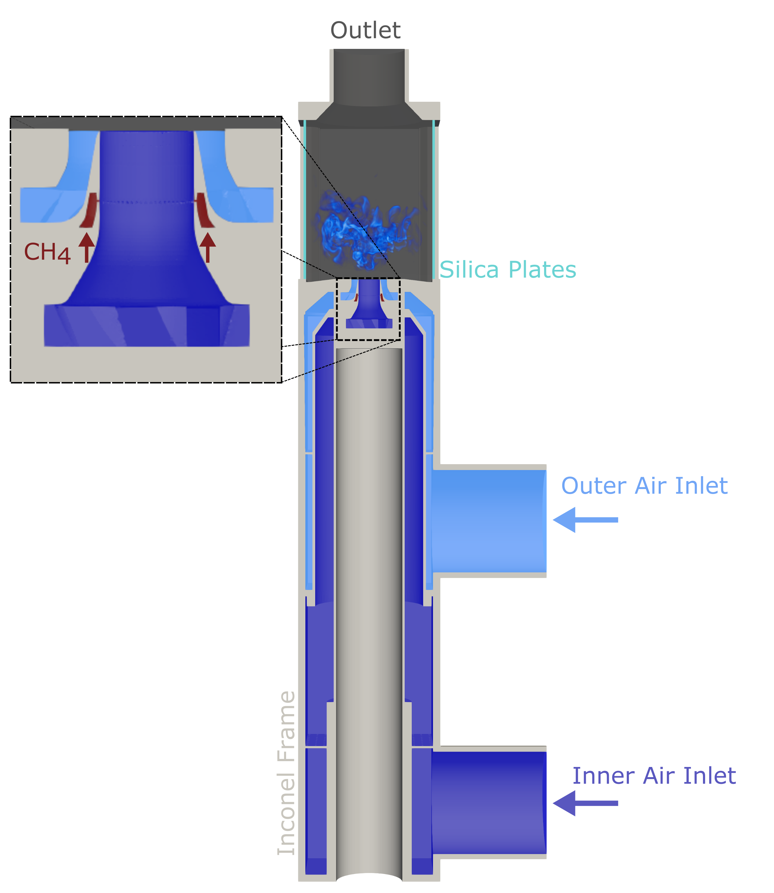
Figure 1: SCHEMATIC OF THE SFB606 GTMC BURNER SHOWING THE DOMAIN USED FOR THE CFD SIMULATIONS.

In this study, the unstable operation point (flame B) of the SFB606 dual swirl GTMC is simulated and compared with experimental data from Arndt et al. [35, 39]. A detailed description of the combustor can be found in [35, 38, 37, 28]; only a brief summary is given here.

A schematic of the burner is shown in Fig. 1. The combustion chamber, with a square cross-section ($$89\text{\,}\mathrm{mm}\text{/}$\times$89\text{\,}\mathrm{mm}\text{/}$$), features a dual swirl injector where each swirler is fed by an individual air intake. Each of these intakes is equipped with a sonic nozzle (not displayed in Fig. 1). The inflow gases are injected into the combustion chamber at ambient pressure and temperature. CH4 is injected into the inner swirler ($D=$15\text{\,}\mathrm{mm}\text{/}$$) $12\text{\,}\mathrm{mm}\text{/}$ below the chamber inlet through 60 holes arranged in a circle with a diameter of $0.5\text{\,}\mathrm{mm}\text{/}$ [35, 38]. The annular outer swirler ($D_{i}=$15.2\text{\,}\mathrm{mm}\text{/}$$, $D_{o}=$24\text{\,}\mathrm{mm}\text{/}$$) provides air only. At the outlet, the burner is connected to the ambient environment through a circular pipe, while optical access is provided by four windows. Pressure oscillations were measured using microphone probes in the combustion chamber and both air inlets. Velocities were measured with stereoscopic particle image velocimetry (PIV) in the centerplane [35]. Single-shot laser Raman scattering was used to deduce the temperature and mass fractions of O2, N2, CH4, H2, CO, CO2 and H2O [35]. The inner wall temperature $T_{w}$ of the silica plates and the metal frame were measured by Arndt et al. [39] using 2D phosphor thermometry.

3 Numerical Model

The LES are performed with an in-house solver integrated into the OpenFOAM framework [41]. For combustion modeling, a flamelet-based tabulated chemistry approach, using premixed manifolds is employed [42] to retrieve the thermo-chemical state during the simulation. The solver was successfully validated in previous works on LES combined with tabulated chemistry[43, 44, 45]. The flow field is described by the Favre-filtered Navier-Stokes equations. Additional transport equations are solved for the mixture fraction $\widetilde{Z}$, the progress variable $\widetilde{Y}_{c}=\widetilde{Y}_{CO_{2}}+\widetilde{Y}_{H_{2}O}$ and the enthalpy $\widetilde{h}$ for the non-adiabatic simulation only. These variables are employed to perform the flamelet table lookup $\widetilde{\Phi}=\Phi^{table}(\widetilde{Z},\widetilde{Y}_{c})$ or $\widetilde{\Phi}=\Phi^{table}(\widetilde{Z},\widetilde{h},\widetilde{Y}_{c})$ in the adiabatic/non-adiabatic LES, respectively. The operator $\widetilde{\cdot}$ denotes the Favre-filtered nature of the solved equations. To account for heat losses in the enthalpy-dependent table, the procedure outlined in [46, 47] is used. Since the reported pressure oscillations are below $1\text{\,}\mathrm{kPa}\text{/}$ [35], the effect of pressure variations on the chemical composition and temperature is assumed negligible [23, 24]. Flamelet tables are generated with the in-house solver ULF [48] from calculations of freely-propagating premixed flames with the GRI-3.0 mechanism[49]. For the adiabatic table, flames are calculated for different mixture fractions and parameterized by $Z$ and the normalized progress variable $Y_{c}^{norm}=(Y_{c}-Y_{c,min})/(Y_{c,max}-Y_{c,min})$. For the enthalpy-dependent table, this step is repeated for different enthalpy levels, which are normalized to $h^{norm}$ analogous to $Y_{c}^{norm}$. The different enthalpy levels are obtained by varying the inlet temperature between $300\text{\,}\mathrm{K}\text{/}$ and $900\text{\,}\mathrm{K}\text{/}$, and by a variable ratio of cooled exhaust gases, which are recirculated and mixed with the unburned mixture at $300\text{\,}\mathrm{K}\text{/}$ in the flamelet calculation. The procedure is explained in detail in [47]. The tables contain 444$\times$101($\times$101 points) in the $Z$, $Y_{c}^{norm}$ and $h^{norm}$ space. Unity Lewis number is assumed for all species.

The effects of unresolved turbulence are accounted for by the $\sigma$ sub-grid model [50] with $c_{\sigma}=1.5$. The turbulence-chemistry interaction is modeled using the ATF approach, following the procedure presented in [51]. In the ATF approach, the flame front is artificially thickened using the thickening factor $\mathcal{F}$, enabling it to be resolved on coarse grids, while preserving the flame propagation. The effect of unresolved flame wrinkling is accounted for by the efficiency function $\mathcal{E}$. Here, the efficiency function formulation developed by Charlette et al. [52] is used. To keep regions of pure mixing unaltered and only thickening the regions where combustion takes place the flame sensor formulated in [53] is used. A grid-adaptive thickening with six grid points in the flame zone is applied following [52].

To account for heat conduction through the solid combustion chamber and the swirler, a loosely coupled simulation of the solid and fluid domain is performed. Calculations of the solid domain were carried out with the OpenFOAM solver chtMultiRegionFoam (v2006), where the enthalpy equation is solved in the solid. Previous studies  [29] showed, that the solid domain is in a steady state as the heat release fluctuations in the fluid are too fast to alter the temperature distribution in the solid. Therefore, the solid domain is simulated separately from the fluid domain, drastically reducing the computational cost. To reach equilibrium between the solid and the time-averaged fluid domain 4 iterations of 30 ms of fluid simulation and a consecutive solid simulation with the fluid heat flux as boundary condition were performed. Further iterations did not alter the resulting temperature field in the solid.

4 Numerical Setup

The numerical domain contains both air inlet sections and the combustion chamber as shown in Fig. 1. The grid contains 17 million cells (mostly hexahedra). A slice of the mesh is shown on top of the time-averaged temperature $\langle\tilde{T}\rangle$ field in Fig. 2. At the inlets, air and methane are injected into the domain at $300\text{\,}\mathrm{K}\text{/}$. The mass flows are $\dot{m}_{air,i}=$282\text{\,}\mathrm{g}\mathrm{/}\min$$, $\dot{m}_{air,o}=$451\text{\,}\mathrm{g}\mathrm{/}\min$$ and $\dot{m}_{CH_{4}}=$30\text{\,}\mathrm{g}\mathrm{/}\min$$ for the inner, outer air and methane inlets, respectively [35]. The pressure $\overline{p}_{far}=$1\text{\,}\mathrm{a}\mathrm{t}\mathrm{m}$$ is prescribed at the outlet with the approximate waveTransmissive boundary condition[41], which models the impedance of an open duct. LES with adiabatic walls are performed using the adiabatic table, while the simulation with isothermal boundary conditions at the chamber walls requires the enthalpy-dependent table. The wall temperature $T_{w}$ on the silica plates and the chamber corners are interpolated from the phosphor thermometry measurements from [39], while the temperature at the burner plate and the swirler wall is determined by CHT calculation.

The solid domain is discretized with 13 million cells. In the CHT calculation, the heat conduction is solved in the solid parts of the burner, namely the silica plates and the Inconel frame. Where available, wall temperatures are interpolated from measurements [39], while the time-averaged heat flux from the fluid domain is used as a boundary condition for the inner wall. At the outer walls of the solid, a heat transfer coefficients of $h=$112\text{\,}\mathrm{W}\text{/}\text{(}{\mathrm{m}}^{2}\text{\,}\mathrm{K}\text{)}$$ and an ambient temperature of $T_{amb}=$300\text{\,}\mathrm{K}\text{/}$$ are set. Both are estimated from the reported heat loss in [39]. The resulting steady-state $T_{w}$ distribution from the solid simulation is mapped onto the fluid simulation and employed as a temperature boundary condition. This procedure was repeated until the temperature distribution in the solid reached a steady state. Afterwards the sampling was conducted over $80\text{\,}\mathrm{m}\mathrm{s}$. Simulations are solved using second-order schemes for space and time discretization.

5 Results

In this section, the time-averaged flow field quantities are first analyzed for both the adiabatic (Adi.) and enthalpy-dependent LES (Enth.). The latter is characterized by isothermal boundary conditions, requiring an enthalpy-depended table. Subsequently, the phase-averaged variables and acoustic cycle obtained in the enthalpy-dependent LES are discussed. The time-averaged temperature $\langle\tilde{T}\rangle$ field of the enthalpy-dependent LES is plotted in Fig. 2. Also shown are the mesh and the coordinate system, which has its origin in the center of the swirler at the burner exit plane. The white lines mark the axial positions at which quantitative comparisons are presented in the following.

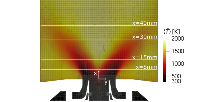
Figure 2: SLICE OF THE TIME-AVERAGED TEMPERATURE FIELD $\langle\tilde{T}\rangle$ OF THE ENTH. DEPENDENT LES. ALSO SHOWN ARE THE COORDINATE SYSTEM, THE GRID AND AXIAL POSITIONS OF QUANTITATIVE COMPARISONS.

5.1 Time-averaged flow field

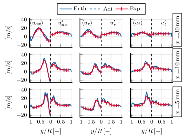
Figure 3: COMPARISON OF TIME-AVERAGED (LEFT) AND RMS (RIGHT) VELOCITY PROFILES BETWEEN SIMULATIONS AND EXPERIMENTAL DATA AT FOUR AXIAL LOCATIONS ($x=$5\text{\,}\mathrm{mm}\text{/}$$, $x=$10\text{\,}\mathrm{mm}\text{/}$$, $x=$20\text{\,}\mathrm{mm}\text{/}$$ AND $x=$30\text{\,}\mathrm{mm}\text{/}$$). FROM LEFT TO RIGHT: AXIAL $u_{ax}$, RADIAL $u_{r}$ AND TANGENTIAL $u_{t}$ VELOCITY COMPONENTS.

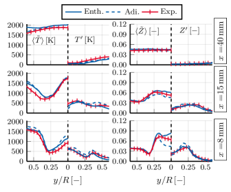
Figure 4: COMPARISON OF TIME-AVERAGED AND RMS TEMPERATURE (LEFT) AND MIXTURE FRACTION (RIGHT) PROFILES BETWEEN SIMULATION AND EXPERIMENTAL DATA AT THREE AXIAL LOCATIONS ($x=$8\text{\,}\mathrm{mm}\text{/}$$, $x=$15\text{\,}\mathrm{mm}\text{/}$$ AND $x=$40\text{\,}\mathrm{mm}\text{/}$$).

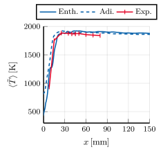
Figure 5: COMPARISON OF TIME-AVERAGED TEMPERATURE PROFILES BETWEEN SIMULATIONS AND EXPERIMENTAL DATA ALONG THE CENTERLINE OF THE COMBUSTOR.

In Fig. 3, the time-averaged velocity profiles obtained by the LES and the experimental measurements are compared at three axial locations (left half of the plots). Good agreement is observed for all velocity components. The position and the value of the velocity peaks are correctly predicted at all axial locations. The simulations accurately reproduce the inner recirculation zone (IRZ) indicated by the negative velocities at $y/R=0$, and the outer recirculation zones (ORZ), marked by negative velocities at $y/R=\pm 1$. The RMS profiles of the velocity are also shown in Fig. 3 (right half of the plots). Overall a very good prediction is observed for both adiabatic and enthalpy-dependent LES.

Figure 4 shows the time-averaged temperature $\langle\widetilde{T}\rangle$ and mixture fraction profile $\langle\widetilde{Z}\rangle$ at three axial positions (left) as well as the RMS values of both variables (right). The adiabatic LES overestimates the temperature in the ORZ regions since heat losses are not accounted for. Furthermore, the flame anchoring is predicted much closer to the inlet as indicated also in the mean temperature profile along the centerline shown in Fig. 5. At $x=$8\text{\,}\mathrm{mm}\text{/}$$ $\langle\tilde{Z}\rangle$ is underpredicted by the adiabatic LES in the center, indicating that the mixture field is not captured accurately. Regarding the enthalpy-dependent LES, it can be seen that at $x=$8\text{\,}\mathrm{mm}\text{/}$$ the temperature at the center of the burner is slightly overestimated due to the prediction of the hot IRZ slightly closer to the chamber inlet. This has also been observed in Fig. 5, which indicates that the profile shifts slightly upstream, towards the inlet, for the enthalpy-dependent LES , although the general shape is well captured.

Figure 6 shows the time-averaged profiles of CO2, CH4, and H2O mass fractions. At $x=$8\text{\,}\mathrm{mm}\text{/}$$, CH4 is severely underpredicted by the adiabatic LES. This is partially caused by an altered mixing field, which transports less fuel to the center of the combustor, indicated by the $\langle\tilde{Z}\rangle$ profile, see Fig. 4, and by the flame anchoring much closer to the inlet plane, see Fig. 5, already consuming CH4. Downstream both simulation results are close to the experimental measurements. The findings showcase that the adiabatic simulation is not able to capture the correct flame anchoring and mixture field, therefore it is not considered for the analysis of the acoustic cycle in the following.

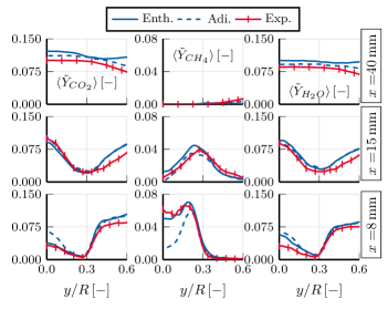
Figure 6: COMPARISON OF TIME-AVERAGED SPECIES MASS FRACTION PROFILES BETWEEN SIMULATION AND EXPERIMENTAL DATA AT THREE AXIAL LOCATIONS ($x=$8\text{\,}\mathrm{mm}\text{/}$$, $x=$15\text{\,}\mathrm{mm}\text{/}$$ AND $x=$40\text{\,}\mathrm{mm}\text{/}$$).

5.2 Analysis of the acoustic cycle

As discussed in the previous section, the time-averaged results over the entire thermo-acoustic cycle indicate good agreement between the enthalpy-dependent LES and experiments. In this section, the pressure response of the burner is first analyzed, then a detailed analysis of the flow field over the different phases in the cycle is conducted.

The Fourier transformed pressure amplitude in the combustion chamber $p_{c}$ calculated in the LES is plotted in Fig. 7 and compared with the measured pressure signal. The dominant frequency of $392\text{\,}\mathrm{Hz}\text{/}$ corresponding to the resonance mode of the inner air intake section [35], is captured closely in the simulation. The other peaks in the experimental spectrum, corresponding to the second harmonic of the dominant mode ($785\text{\,}\mathrm{Hz}\text{/}$) and the Helmholtz frequency of the combustor and outer plenum ($139\text{\,}\mathrm{Hz}\text{/}$)[35], are not captured by the simulation. Previous studies on a similar burner configuration suggested that the side glass walls could significantly dampen pressure amplitudes [40], depending on their mounting design.

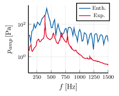
Figure 7: CALCULATED AND MEASURED PRESSURE SPECTRA INSIDE THE COMBUSTION CHAMBER.

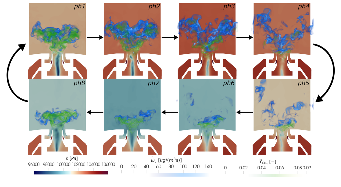
Figure 8: VISUALIZATION OF THE FEEDBACK CYCLE WITH VOLUME PLOTS OF METHANE MASS FRACTION $\widetilde{Y}_{CH_{4}}$ AND PROGRESS VARIABLE SOURCE TERM $\widetilde{\dot{\omega}}_{c}$. THE COLORED AREA IN THE CENTRAL PLANE INDICATES THE PRESSURE $\overline{p}$.

Experimental investigations in [35, 12] showed that equivalence ratio oscillation coupled with a convective time delay contribute to the thermoacoustic feedback mechanisms.

The LES reproduces the same behavior. To analyze the feedback mechanism in detail, a single cycle is shown in Fig. 8, where eight snapshots are arranged from a phase angle of $0^{\circ}$ (ph1) for the sin-pressure signal to a phase angle of $337.5^{\circ}$ (ph8), similarly to the experimental measurements from [35]. Each snapshot features the instantaneous three-dimensional progress variable source term, the mass fraction of methane and the pressure contour on the center plane.

For quantitative analysis, the phase-conditioned averaged velocity field has been calculated for the eight phases following the procedure outlined in [35], i.e. samples are sorted and averaged in a $45^{\circ}$ phase angle range around the previously defined phase centers and compared with the phase-conditioned averaged experimental data in Fig. 9. The symmetry of the combustion chamber was utilized to increase the number of samples, gathered over $31\text{\,}\mathrm{ms}\text{/}$ of simulated time.

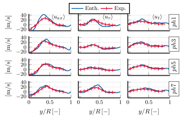
Figure 9: COMPARISON OF PHASE-AVERAGED VELOCITY PROFILES AT $x=$15\text{\,}\mathrm{mm}\text{/}$$. FROM LEFT TO RIGHT AXIAL: $u_{ax}$, RADIAL $u_{r}$ AND TANGENTIAL $u_{t}$ VELOCITY COMPONENTS.

A PVC structure can be observed in the low-pressure region inside the swirler over all phases. ph3 corresponds to the phase with the highest chamber pressure, while ph7 features the lowest pressure. In ph3 the high pressure is linked to a large flame zone which has a visible V-shape in Fig. 8. Due to the high chamber pressure, the driving pressure difference between the plenum and the chamber $\Delta P$ is low and the velocity inside the swirler and plenum decreases, leading to the accumulation of fuel inside the swirler close to the inlet, slimilarly to [12, 40]. In ph4 and ph5, the flame zone is convected downstream until the fuel is completely consumed. In these phases the flame interacts with the chamber walls, see Fig. 8. Up to ph7, the chamber pressure drops and the flame zone is in the center of the burner close to the inlet, where the fresh mixture accumulates. At ph7 the pressure difference between chamber and plenum is largest, accelerating the gas inside the swirler, which in turn convects the fuel-rich mixture into the chamber, where a larger flame zone forms in the subsequent phases. The thermal expansion of the gas then leads to an increase in chamber pressure and a consequent decrease in the pressure difference $\Delta P$.

The phase-averaged velocity components shown in Fig. 9 indicate that at ph7 the simulation features higher radial velocities compared to the experiments at the reference location $x=$15\text{\,}\mathrm{mm}\text{/}$$. Axial velocity peaks are overestimated until ph3. Here, the LES predicts the measured velocity accurately. This indicates that the stronger pressure oscillations predicted by the simulation, yield higher inflow velocities in the phases of low but rising pressures.

Figure 10 shows the mixture fraction PDF $P(Z)$ over the phases at the axial location $x=$15\text{\,}\mathrm{mm}\text{/}$$ compared with the measurements. From ph3 to ph6, the LES predicts a slightly different profile of the mixture fraction PDF, overestimating the peak value and underestimating the peak position. Figure 11 shows the conditional mean of the temperature with respect to the mixture fraction. Here good agreement with the experimental data is observed except for ph5 to ph7, where the temperature is overpredicted for high mixture fraction values. Contrary to the experiment, pockets of high mixture fraction already enter the flame zone or the hot recirculation zone, which does not occur in the experiment. The deviations between the LES and experiments in the mixture fraction-conditioned temperature are shifted compared to the deviations in $P(Z)$ by two phases. These results indicate that although the frequency of the oscillation is reproduced well in the simulation, slight differences in the flame behavior are still observable due to the overestimated amplitude of the oscillation. Further investigations to address this issue will be scope of future studies.

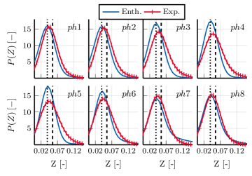
Figure 10: PHASE-AVERAGED MIXTURE FRACTION PDF AT $x=$15\text{\,}\mathrm{mm}\text{/}$$. DASHED AND DOTTED LINES MARK THE STOICHIOMETRIC AND GLOBAL MIXTURE FRACTION, RESPECTIVELY.

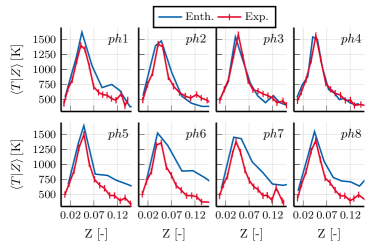
Figure 11: TEMPERATURE CONDITIONED ON MIXTURE FRACTION OVER THE DIFFERENT PHASES AT $x=$15\text{\,}\mathrm{mm}\text{/}$$.

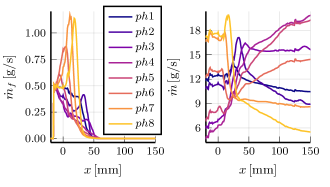
Figure 12: CROSS SECTION AND PHASE-AVERAGED PROFILES OF FUEL MASS FLOW $\dot{m}_{f}$ AND GLOBAL MASS FLOW $\dot{m}$.

To better understand the nature of the acoustic coupling to convective time delay, the fuel mass flow $\dot{m}_{f}$ and the global mass flow $\dot{m}$ averaged over cross-sections and phases are plotted in Fig. 12. The $\dot{m}_{f}$ phase profiles indicate that the fuel injected into the burner (injection holes at $x=$-12\text{\,}\mathrm{mm}\text{/}$$) is constant over all phases, supporting the hypothesis in [12, 35] that the fuel stream at the injection holes is not influenced by the acoustic cycle due to the high-pressure loss experienced during the injection process. CH4 accumulates downstream and is convected in larger quantities through the chamber in the low-pressure phase (ph7) while it is consumed in the high-pressure phase (ph3). Up to $x=$10\text{\,}\mathrm{mm}\text{/}$$ the overall mass flow $\dot{m}$ on the contrary does not change with $x$ for all phases. For $x>$10\text{\,}\mathrm{mm}\text{/}$$ a distinct peak is observed between ph8 and ph2 only. To further analyze the convective delay, the mass flows and the progress variable source term are plotted over the phase angle in Fig. 13 for different axial positions. The pressure fluctuation is also shown. The evolution of $\dot{m}_{f}$ shows a shift in the peak towards higher phase angles with increasing axial position, while $\dot{m}$ features overlapping sinus signals from $x=$-5\text{\,}\mathrm{mm}\text{/}$$ to $x=$5\text{\,}\mathrm{mm}\text{/}$$, 40^∘ behind $p$, while a convective delay is observed for $\dot{m}$ for $x>$10\text{\,}\mathrm{mm}\text{/}$$. This confirms that the fuel flow experiences a convective delay already inside the swirler. The convective time delay of $\dot{m}_{f}$ between $x=$-5\text{\,}\mathrm{mm}\text{/}$$ and $x=$0\text{\,}\mathrm{mm}\text{/}$$ corresponds to $\Delta t=\Delta x/u_{ax}=$0.17\text{\,}\mathrm{ms}\text{/}$$, close to the observed phase delay of 25^∘($0.174\text{\,}\mathrm{ms}\text{/}$). Between $x=$-5\text{\,}\mathrm{mm}\text{/}$$ and $x=$15\text{\,}\mathrm{mm}\text{/}$$ the shift between $\dot{m}_{f}$ and the $\dot{m}$ peak shrinks from 90^∘ to only 18^∘. At $x=$40\text{\,}\mathrm{mm}\text{/}$$ both are in phase of each other having experienced a similar convective delay from $x=$15\text{\,}\mathrm{mm}\text{/}$$. The progress variable source term $\dot{\omega}_{Y_{c}}$ in Fig. 13 showcases a high reaction rate over the entire cycle, with a broad peak around 0^∘, 60^∘($0.416\text{\,}\mathrm{ms}\text{/}$) earlier than the $\dot{m}_{f}$ peak for $x=$15\text{\,}\mathrm{mm}\text{/}$$. The peak corresponds to the compact flame in ph1 (Fig. 8). For $x=$40\text{\,}\mathrm{mm}\text{/}$$ $\dot{\omega}_{Y_{c}}$ is limited to a broad peak around 135^∘.

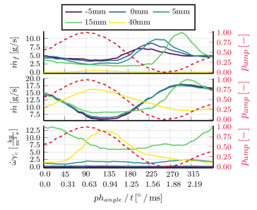
Figure 13: CROSS-SECTION AND PHASE-AVERAGED PROFILES OF FUEL MASS FLOW $\dot{m}_{f}$, GLOBAL MASS FLOW $\dot{m}$ AND PROGRESS VARIABLE SOURCE TERM $\dot{\omega}_{Y_{c}}$ OVER THE PHASE ANGLE AT DIFFERENT AXIAL POSITIONS. THE PRESSURE SIGNAL IS INDICATED BY THE DASHED LINE.

6 Conclusions

This study numerically investigated the thermo-acoustic unstable operating point B of the SFB606 GTMC using LES. In one simulation adiabatic walls were assumed, while in a second LES isothermal walls with temperatures interpolated from measurements and a coupled CHT simulation to account for the heat losses were considered. Both simulations employed a correspondent tabulated chemistry manifold coupled with the ATF model for the turbulent combustion closure. The following conclusions can be drawn based on this study:

1. For the adiabatic LES a flame anchoring point much closer to the inlet plane and an altered mixture field was observed. Therefore, further phase-conditioned analysis with the adiabatic LES are not conducted.

2. The enthalpy-dependent LES is able to closely predict the time-averaged profiles and frequency of the dominant mode, validating the employed numerical methodology as a viable tool to simulate thermo-acoustic oscillations and capture the feedback mechanism qualitatively. An equivalence ratio oscillation coupled to the dominant mode through a convective time delay, which is different from the delay of the overall mass flux, is observed and contributes to the feedback mechanism of the thermo-acoustic coupling.

3. For the first time, the phase-conditioned velocities, mixture fraction PDF and conditional temperature, have been compared with phase-conditioned PIV and Raman measurements for the enthalpy-dependent simulation. The presented numerical framework showcases fair quantitative agreement with the phase-averaged measurements, although small deviations in the pressure amplitude and phase-dependent mixing field are observed.

4. The fuel mass flow injected into the swirler is not affected by the pressure oscillations, as suggested by Arndt et al. [35]. Contrary to the global mass flux a convective delay of the fuel mass flux peak is already observable inside the swirler.

In summary, the results clearly show that the LES considering heat transfer effects is able to predict the global flow field more accurately than the adiabatic simulation. Further, the highly unsteady flame dynamics are captured with sufficient precision by the non-adiabatic LES, which is indispensable for the prediction of combustion instabilities.

7 Acknowledgements

Calculations for this research were conducted on the Lichtenberg high-performance computer at TU Darmstadt. This research was part of the ”Center of Excellence in Combustion”, which received funding from the European Union’s Horizon 2020 research and innovation program under grant agreement No^∘ 952181.

References

- Huang and Yang [2009] Y. Huang and V. Yang. Dynamics and stability of lean-premixed swirl-stabilized combustion. Prog. Energy Combust. Sci., 35(4):293–364, 2009. doi: 10.1016/j.pecs.2009.01.002.
- Gicquel et al. [2012] L. Y. M. Gicquel, G. Staffelbach, and T. Poinsot. Large eddy simulations of gaseous flames in gas turbine combustion chambers. Prog. Energy Combust. Sci., 38(6):782–817, 2012. doi: 10.1016/j.pecs.2012.04.004.
- Oberleithner et al. [2015] K. Oberleithner, M. Stöhr, S. H. Im, C. M. Arndt, and A. M. Steinberg. Formation and flame-induced suppression of the precessing vortex core in a swirl combustor: Experiments and linear stability analysis. Combust. Flame, 162(8):3100–3114, 2015. doi: 10.1016/j.combustflame.2015.02.015.
- Poinsot [2017] T. Poinsot. Prediction and control of combustion instabilities in real engines. Proc. Combust. Inst., 36(1):1–28, 2017. doi: 10.1016/j.proci.2016.05.007.
- Schuller et al. [2003] T. Schuller, D. Durox, and S. Candel. Self-induced combustion oscillations of laminar premixed flames stabilized on annular burners. Combust. Flame, 135(4):525–537, 2003. ISSN 00102180. doi: 10.1016/j.combustflame.2003.08.007.
- Lieuwen and Yang [2006] T. C. Lieuwen and V. Yang. Combustion Instabilities In Gas Turbine Engines. AAIA, Reston ,VA, 2006. ISBN 978-1-56347-669-3. doi: 10.2514/4.866807. URL http://arc.aiaa.org/doi/book/10.2514/4.866807.
- Schadow and Gutmark [1992] K. C. Schadow and E. Gutmark. Combustion instability related to vortex shedding in dump combustors and their passive control. Prog. Energy Combust. Sci., 18(2):117–132, 1992. ISSN 03601285. doi: 10.1016/0360-1285(92)90020-2.
- Palies et al. [2011] P. Palies, T. Schuller, D. Durox, L. Y. Gicquel, and S. Candel. Acoustically perturbed turbulent premixed swirling flames. Phys. Fluids, 23(3), 2011. ISSN 10706631. doi: 10.1063/1.3553276.
- Boxx et al. [2012] I. Boxx, C. M. Arndt, C. D. Carter, and W. Meier. High-speed laser diagnostics for the study of flame dynamics in a lean premixed gas turbine model combustor. Exp. Fluids, 52:555–567, 2012. ISSN 0723-4864. doi: 10.1007/s00348-010-1022-x.
- Stöhr et al. [2018] M. Stöhr, K. Oberleithner, M. Sieber, Z. Yin, and W. Meier. Experimental study of transient mechanisms of bistable flame shape transitions in a swirl combustor. J. Eng. Gas Turbines Power, 140, 2018. ISSN 0742-4795. doi: 10.1115/1.4037724.
- Lieuwen and Zinn [1998] T. Lieuwen and B. T. Zinn. The role of equivalence ratio oscillations in driving combustion instabilities in low NOx gas turbines. Symp. (Int.) Combust., 27(2):1809–1816, 1998. ISSN 00820784. doi: 10.1016/S0082-0784(98)80022-2.
- Meier et al. [2007] W. Meier, P. Weigand, X. R. Duan, and R. Giezendanner-Thoben. Detailed characterization of the dynamics of thermoacoustic pulsations in a lean premixed swirl flame. Combust. Flame, 150:2–26, 2007. ISSN 0010-2180. doi: 10.1016/j.combustflame.2007.04.002.
- Kim et al. [2010] K. Kim, J. Lee, B. Quay, and D. Santavicca. Response of partially premixed flames to acoustic velocity and equivalence ratio perturbations. Combust. Flame, 157(9):1731–1744, 2010. doi: 10.1016/j.combustflame.2010.04.006.
- Ćosić et al. [2015] B. Ćosić, S. Terhaar, J. P. Moeck, and C. O. Paschereit. Response of a swirl-stabilized flame to simultaneous perturbations in equivalence ratio and velocity at high oscillation amplitudes. Combust. Flame, 162(4):1046–1062, 2015. doi: 10.1016/j.combustflame.2014.09.025.
- Weigand et al. [2006a] P. Weigand, W. Meier, X. R. Duan, W. Stricker, and M. Aigner. Investigations of swirl flames in a gas turbine model combustor. Combust. Flame, 144(1-2):205–224, 2006a. doi: 10.1016/j.combustflame.2005.07.010.
- Meier et al. [2006] W. Meier, X. R. Duan, and P. Weigand. Investigations of swirl flames in a gas turbine model combustor. Combust. Flame, 144(1-2):225–236, 2006. doi: 10.1016/j.combustflame.2005.07.009.
- Weigand et al. [2006b] P. Weigand, W. Meier, X. Duan, and M. Aigner. Laser based investigations of thermo-acoustic instabilities in a lean premixed gas turbine model combustor. In Volume 1: Combustion and Fuels, Education, pages 237–245. ASME, 2006b. doi: 10.1115/gt2006-90300.
- Raman and Hassanaly [2019] V. Raman and M. Hassanaly. Emerging trends in numerical simulations of combustion systems. Proc. Combust. Inst., 37(2):2073–2089, 2019. ISSN 15407489. doi: 10.1016/j.proci.2018.07.121.
- Roux et al. [2005] S. Roux, G. Lartigue, T. Poinsot, U. Meier, and C. Bérat. Studies of mean and unsteady flow in a swirled combustor using experiments, acoustic analysis, and large eddy simulations. Combust. Flame, 141(1-2):40–54, 2005. doi: 10.1016/j.combustflame.2004.12.007.
- Franzelli et al. [2012] B. Franzelli, E. Riber, L. Y. M. Gicquel, and T. Poinsot. Large eddy simulation of combustion instabilities in a lean partially premixed swirled flame. Combust. Flame, 159(2):621–637, 2012. doi: 10.1016/j.combustflame.2011.08.004.
- Galpin et al. [2008] J. Galpin, A. Naudin, L. Vervisch, C. Angelberger, O. Colin, and P. Domingo. Large-eddy simulation of a fuel-lean premixed turbulent swirl-burner. Combust. Flame, 155(1-2):247–266, 2008. doi: 10.1016/j.combustflame.2008.04.004.
- Wang et al. [2014] P. Wang, N. Platova, J. Fröhlich, and U. Maas. Large eddy simulation of the PRECCINSTA burner. Int. J. Heat and Mass Transfer, 70:486–495, 2014. doi: 10.1016/j.ijheatmasstransfer.2013.11.025.
- See and Ihme [2015] Y. C. See and M. Ihme. Large eddy simulation of a partially-premixed gas turbine model combustor. Proc. Combust. Inst., 35(2):1225–1234, 2015. doi: 10.1016/j.proci.2014.08.006.
- Gövert et al. [2017] S. Gövert, D. Mira, J. B. W. Kok, M. Vázquez, and G. Houzeaux. The effect of partial premixing and heat loss on the reacting flow field prediction of a swirl stabilized gas turbine model combustor. Flow Turbul. Combust., 100(2):503–534, 2017. doi: 10.1007/s10494-017-9848-4.
- [25] D. Fredrich, W. Jones, and A. J. Marquis. The stochastic fields method applied to a partially premixed swirl flame with wall heat transfer. 205:446–456. doi: 10.1016/j.combustflame.2019.04.012.
- Donini et al. [2016] A. Donini, R. J. M. Bastiaans, J. A. van Oijen, and L. P. H. de Goey. A 5-d implementation of FGM for the large eddy simulation of a stratified swirled flame with heat loss in a gas turbine combustor. Flow Turbul. Combust., 98(3):887–922, 2016. doi: 10.1007/s10494-016-9777-7.
- Benard et al. [2019] P. Benard, G. Lartigue, V. Moureau, and R. Mercier. Large-eddy simulation of the lean-premixed PRECCINSTA burner with wall heat loss. Proc. Combust. Inst., 37(4):5233–5243, 2019. doi: 10.1016/j.proci.2018.07.026.
- Kraus et al. [2017] C. Kraus, L. Selle, T. Poinsot, C. M. Arndt, and H. Bockhorn. Influence of heat transfer and material temperature on combustion instabilities in a swirl burner. J. Eng. Gas Turbines Power, 139, 2017. ISSN 0742-4795. doi: 10.1115/1.4035143.
- Kraus et al. [2018] C. Kraus, L. Selle, and T. Poinsot. Coupling heat transfer and large eddy simulation for combustion instability prediction in a swirl burner. Combust. Flame, 191:239–251, 2018. ISSN 0010-2180. doi: 10.1016/j.combustflame.2018.01.007.
- Tang and Raman [2021] Y. Tang and V. Raman. Large eddy simulation of premixed turbulent combustion using a non-adiabatic, strain-sensitive flamelet approach. Combust. Flame, 234:111655, 2021. ISSN 00102180. doi: 10.1016/j.combustflame.2021.111655. URL https://www.sciencedirect.com/science/article/pii/S0010218021003989https://linkinghub.elsevier.com/retrieve/pii/S0010218021003989.
- Agostinelli et al. [2021] P. W. Agostinelli, D. Laera, I. Boxx, L. Gicquel, and T. Poinsot. Impact of wall heat transfer in Large Eddy Simulation of flame dynamics in a swirled combustion chamber. Combust. Flame, 234:111728, 2021. ISSN 15562921. doi: 10.1016/j.combustflame.2021.111728. URL https://doi.org/10.1016/j.combustflame.2021.111728.
- Tay-wo chong et al. [2017] L. Tay-wo chong, A. Scarpato, and W. Polifke. LES combustion model with stretch and heat loss effects for prediction pf premixed flame characteristics and dynamics. pages 1–12. GT2017-63357 ASME, 2017.
- Massey et al. [2021] J. C. Massey, Z. X. Chen, and N. Swaminathan. Modelling Heat Loss Effects in the Large Eddy Simulation of a Lean Swirl-Stabilised Flame. Flow, Turbul. Combust., 106(4):1355–1378, 2021. ISSN 15731987. doi: 10.1007/s10494-020-00192-4. URL https://doi.org/10.1007/s10494-020-00192-4.
- Tay-Wo-Chong and Polifke [2012] L. Tay-Wo-Chong and W. Polifke. LES-based study of the influence of thermal boundary condition and combustor confinement on premix flame transfer functions. In Proc. ASME Turbo Expo 2012, pages 579–588. ASME, 2012. doi: 10.1115/gt2012-68796.
- Arndt et al. [2015] C. M. Arndt, M. Severin, C. Dem, M. Stöhr, A. M. Steinberg, and W. Meier. Experimental analysis of thermo-acoustic instabilities in a generic gas turbine combustor by phase-correlated PIV, chemiluminescence, and laser raman scattering measurements. Exp. Fluids, 56(4), 2015. ISSN 0723-4864. doi: 10.1007/s00348-015-1929-3.
- Meier et al. [2016] W. Meier, C. Dem, and C. M. Arndt. Mixing and reaction progress in a confined swirl flame undergoing thermo-acoustic oscillations studied with laser raman scattering. Exp. Therm. Fluid Sci., 73:71–78, 2016. ISSN 0894-1777. doi: 10.1016/j.expthermflusci.2015.09.011.
- Kraus et al. [2016] C. Kraus, S. Harth, and H. Bockhorn. Experimental investigation of combustion instabilities in lean swirl-stabilized partially-premixed flames in single- and multiple-burner setup. Int. J. Spray Combust. Dyn., 8:4–26, 2016. ISSN 1756-8277. doi: 10.1177/1756827715627064.
- Arndt et al. [2017] C. M. Arndt, M. Stöhr, M. J. Severin, C. Dem, and W. Meier. Influence of air staging on the dynamics of a precessing vortex core in a dual swirl gas turbine model combustor. In 53rd AIAA/SAE/ASEE Joint Propulsion Conference. AIAA, 2017. doi: 10.2514/6.2017-4683.
- Arndt et al. [2020] C. M. Arndt, P. Nau, and W. Meier. Characterization of wall temperature distributions in a gas turbine model combustor measured by 2d phosphor thermometry. Proc. Combust. Inst., pages 1867–1875, 2020. doi: 10.1016/j.proci.2020.06.088.
- Lourier et al. [2017] J.-M. Lourier, M. Stöhr, B. Noll, S. Werner, and A. Fiolitakis. Scale adaptive simulation of a thermoacoustic instability in a partially premixed lean swirl combustor. Combust. Flame, 183:343–357, 2017. doi: 10.1016/j.combustflame.2017.02.024.
- OpenFOAM [2013] OpenFOAM. The open source cfd toolbox, openfoam, 2013. URL http://www.openfoam.com.
- van Oijen and de Goey [2000] J. A. van Oijen and L. P. H. de Goey. Modelling of Premixed Laminar Flames using Flamelet-Generated Manifolds Modelling of Premixed Laminar Flames using Flamelet-Generated Manifolds. Combust. Sci. Technol., 161:113–137, 2000. doi: 10.1080/00102200008935814.
- Popp et al. [2015] S. Popp, F. Hunger, S. Hartl, D. Messig, B. Coriton, J. H. Frank, F. Fuest, and C. Hasse. LES flamelet-progress variable modeling and measurements of a turbulent partially-premixed dimethyl ether jet flame. Combust. Flame, 162(8):3016–3029, 2015. doi: 10.1016/j.combustflame.2015.05.004.
- Gierth et al. [2018] S. Gierth, F. Hunger, S. Popp, H. Wu, M. Ihme, and C. Hasse. Assessment of differential diffusion effects in flamelet modeling of oxy-fuel flames. Combust. Flame, 197:134–144, 2018. doi: 10.1016/j.combustflame.2018.07.023.
- Popp et al. [2021] S. Popp, S. Hartl, D. Butz, D. Geyer, A. Dreizler, L. Vervisch, and C. Hasse. Assessing multi-regime combustion in a novel burner configuration with large eddy simulations using tabulated chemistry. Proc. Combust. Inst., 38(2):2551–2558, 2021. ISSN 15407489. doi: 10.1016/j.proci.2020.06.098. URL https://doi.org/10.1016/j.proci.2020.06.098https://linkinghub.elsevier.com/retrieve/pii/S1540748920301589.
- Ketelheun et al. [2013] A. Ketelheun, G. Kuenne, and J. Janicka. Heat transfer modeling in the context of large eddy simulation of premixed combustion with tabulated chemistry. Flow Turbul. Combust., 91(4):867–893, 2013. doi: 10.1007/s10494-013-9492-6.
- Steinhausen et al. [2020] M. Steinhausen, Y. Luo, S. Popp, C. Strassacker, T. Zirwes, H. Kosaka, F. Zentgraf, U. Maas, A. Sadiki, A. Dreizler, and C. Hasse. Numerical investigation of local heat-release rates and thermo-chemical states in side-wall quenching of laminar methane and dimethyl ether flames. Flow Turbul. Combust., page 681–700, 2020. doi: 10.1007/s10494-020-00146-w.
- Zschutschke et al. [2017] A. Zschutschke, D. Messig, A. Scholtissek, and C. Hasse. Universal laminar flame solver (ulf). 2017. doi: 10.6084/m9.figshare.5119855.v2. URL https://figshare.com/articles/poster/ULF_code_pdf/5119855.
- [49] G. P. Smith, D. M. Golden, M. Frenklach, N. W. Moriarty, B. Eiteneer, M. Goldenberg, C. T. Bowman, R. K. Hanson, S. Song, W. C. Gardiner, J. V. V. Lissianski, and Z. Qin. Gri-mech 3.0. URL http://combustion.berkeley.edu/gri-mech/version30/text30.html.
- Nicoud et al. [2011] F. Nicoud, H. B. Toda, O. Cabrit, S. Bose, and J. Lee. Using singular values to build a subgrid-scale model for large eddy simulations. Phys. Fluids, 23, 2011. doi: 10.1063/1.3623274.
- Colin et al. [2000] O. Colin, F. Ducros, D. Veynante, and T. Poinsot. A thickened flame model for large eddy simulations of turbulent premixed combustion. Phys. Fluids, 12(7):1843–1863, 2000. ISSN 1070-6631. doi: 10.1063/1.870436. URL http://aip.scitation.org/doi/10.1063/1.870436.
- Charlette et al. [2002] F. Charlette, C. Meneveau, and D. Veynante. A power-law flame wrinkling model for les of premixed turbulent combustion part i: non-dynamic formulation and initial tests. Combust. Flame, 131:159–180, 2002. ISSN 0010-2180. doi: 10.1016/s0010-2180(02)00400-5.
- Popp et al. [2019] S. Popp, G. Kuenne, J. Janicka, and C. Hasse. An extended artificial thickening approach for strained premixed flames. Combust. Flame, 206:252–265, 2019. ISSN 0010-2180. doi: 10.1016/j.combustflame.2019.04.047.