On the stability and convergence of Physics Informed Neural Networks

Abstract

Physics Informed Neural Networks is a numerical method which uses neural networks to approximate solutions of partial differential equations. It has received a lot of attention and is currently used in numerous physical and engineering problems. The mathematical understanding of these methods is limited, and in particular, it seems that, a consistent notion of stability is missing. Towards addressing this issue we consider model problems of partial differential equations, namely linear elliptic and parabolic PDEs. We consider problems with different stability properties, and problems with time discrete training. Motivated by tools of nonlinear calculus of variations we systematically show that coercivity of the energies and associated compactness provide the right framework for stability. For time discrete training we show that if these properties fail to hold then methods may become unstable. Furthermore, using tools of $\Gamma-$convergence we provide new convergence results for weak solutions by only requiring that the neural network spaces are chosen to have suitable approximation properties.

1 Introduction

1.1 PDEs and Neural Networks

In this work we consider model problems of partial differential equations (PDEs) approximated by deep neural learning (DNN) algorithms. In particular we focus on linear elliptic and parabolic PDEs and Physics Informed Neural Networks, i.e., algorithms where the discretisation is based on the minimisation of the $L^{2}$ norm of the residual over a set of neural networks with a given architecture. Standard tools of numerical analysis assessing the quality and performance of an algorithm are based on the notions of stability and approximability. Typically, in problems arising in scientific applications another important algorithmic characteristic is the preservation of key qualitative properties of the simulating system at the discrete level. In important classes of problems, stability and structural consistency are often linked. Our aim is to introduce a novel notion of stability for the above DNN algorithms approximating solutions of PDEs. In addition, we show convergence provided that the set of DNNs has the right approximability properties and the training of the algorithm produces stable approximations.

In the area of machine learning for models described by partial differential equations, at present, there is intense activity at multiple fronts: developing new methods for solving differential equations using neural networks, designing special neural architectures to approximate families of differential operators (operator learning), combination of statistical and machine learning techniques for related problems in uncertainty quantification and statistical functional inference. Despite the progress at all these problems in the last years, basic mathematical, and hence algorithmical, understanding is still under development.

Partial Differential Equations (PDEs) has been proven an area of very important impact in science and engineering, not only because many physical models are described by PDEs, but crucially, methods and techniques developed in this field contributed to the scientific development in several areas where very few scientists would have guessed as possible. Numerical solution of PDEs utilising neural networks is at an early stage and has received a lot of attention. Such methods have significantly different characteristics compared to more traditional methods, and have been proved quite effective, e.g., in solving problems in high-dimensions, or when methods combining statistical approaches and PDEs are needed. Physics Informed Neural Networks is one of the most successful numerical methods which uses neural networks to approximate solutions of PDEs, see e.g., [39], [33]. Residual based methods were considered in [29], [6], [40], [46] and their references. Other neural network methods for differential equations and related problems include, for example, [41], [18], [27], [48], [12], [20], [23]. The term Physics Informed Neural Networks was introduced in the highly influential paper [39]. It was then used extensively in numerous physical and engineering problems; for a broader perspective of the related methodologies and the importance of the NN methods for scientific applications, see e.g., [26]. Despite progress at some fronts, see [46], [3], [44], [45], [35, 36], the mathematical understanding of these methods is limited. In particular, it seems that, a consistent notion of stability is missing. Stability is an essential tool, in a priori error analysis and convergence of the algorithms, [30]. It provides valuable information for fixed values of the discretisation parameters, i.e., in the pre-asymptotic regime, and it is well known that unstable methods have poor algorithmic performance. On the other hand, stability is a problem dependent notion and not always easy to identify. Towards addressing this issue we consider model problems of partial differential equations, namely linear elliptic and parabolic PDEs. We consider PDEs with different stability properties, and parabolic problems with time discrete training. Since, apparently, the training procedure influences the behaviour of the method in an essential manner, but, on the other hand, complicates the analysis considerably, we have chosen as a first step in this work to consider time discrete only training. Motivated by tools of nonlinear calculus of variations we systematically show that coercivity of the energies and associated compactness provide the right framework for stability. For time discrete training we show that if these properties fail to hold then methods become unstable and it seems that they do not converge. Furthermore, using tools of $\Gamma-$convergence we provide new convergence results for weak solutions by only requiring that the neural network spaces are chosen to have suitable approximation properties.

1.2 Model problems and their Machine Learning approximations

In this work we consider linear elliptic and parabolic PDEs. To fix notation, we consider simple boundary value problems of the form,

$$\left\{\begin{aligned} &L\,u=f\quad&&\text{in}\,\,&&\varOmega\\[2.0pt] &u=0\quad&&\text{on}\,\,&&\partial\varOmega\\[2.0pt] \end{aligned}\right.$$ (1)

where $u:\Omega\subset\mathbb{R}^{d}\rightarrow\mathbb{R},\>\Omega$ is an open, bounded set with smooth enough boundary, $f\in L^{2}(\Omega)$ and $L$ a self-adjoint elliptic operator of the form

$$\begin{gathered}Lu:=-\sum_{1\leq i,j\leq d}\big{(}a_{ij}u_{x_{i}}\big{)}_{x_{j}}+cu\\ \textrm{where}\;\>\sum_{i,j}a_{ij}(x)\xi_{i}\xi_{j}\geq\theta|\xi|^{2}\;\;\textrm{for any}\;\>x\in\Omega\;\>\textrm{and any}\;\>\xi\in\mathbb{R}^{n},\;\;\;\textrm{for some}\;\>\theta>0\end{gathered}$$ (2)

also, $a_{ij}=a_{ji}\in C^{1}(\overline{\Omega}),\>b_{i},\>c\in L^{\infty}(\Omega)$ and hence bounded in $\overline{\Omega}.$ Further assumptions on $L$ will be discussed in the next sections. Dirichlet boundary conditions were selected for simplicity. The results of this work can be extended to other boundary conditions with appropriate technical modifications.

We shall study the corresponding parabolic problem as well. We use the compact notation $\Omega_{T}=\Omega\times(0,T],$ $\partial\Omega_{T}=\partial\Omega\times(0,T]$ for some fixed time $T>0.$ We consider the initial-boundary value problem

$$\begin{cases}u_{t}+Lu=f,\;\;\;\;\textrm{in}\;\>\Omega_{T},\\ u=0,\;\;\;\;\;\;\;\;\;\;\textrm{on}\;\>\partial\Omega\times(0,T],\\ u=u^{0},\;\;\;\;\;\;\;\;\;\;\;\;\textrm{in}\;\>\Omega\,,\end{cases}$$ (3)

where $f\in L^{2}(\Omega_{T}),\;u^{0}\in H^{1}_{0}(\Omega)$ and $L$ is as in (2). In the sequel we shall use the compact operator notation ${\mathscr{L}}$ for either $u_{t}+Lu$ or $Lu$ for the parabolic or the elliptic case correspondingly. The associated energies used will be the $L^{2}-$residuals

$$\mathcal{E}(v)=\int_{\Omega_{D}}|{\mathscr{L}}v-f|^{2}{\mathrm{d}}\overline{x}+\,\mu\int_{\Omega}|v-u^{0}|^{2}\,{\mathrm{d}}x+\tau\,\int_{\partial\Omega_{T}}|v|^{2}\,{\mathrm{d}}\overline{S}$$ (4)

defined over smooth enough functions and domains $\Omega_{D}$ being $\Omega_{T}$ or $\Omega$ (with measures $d\overline{x}\$) for the parabolic or the elliptic case correspondingly. Clearly, the coefficient $\mu\geq 0$ of the initial condition is set to zero in the elliptic case.

It is typical to consider regularised versions of $\mathcal{E}(v)$ as well. Such functionals have the form

$$\mathcal{E}_{reg}(v)=\mathcal{E}(v)+\lambda\mathcal{J}(v)\,,$$ (5)

where the regularisation parameter $\lambda=\lambda_{reg}>0$ is in principle small and $\mathcal{J}(v)$ is an appropriate functional (often a power of a semi-norm) reflecting the qualitative properties of the regularisation. The formulation of the method extends naturally to nonlinear versions of the generic operator ${\mathscr{L}}v-f,$ whereby in principle both ${\mathscr{L}}$ and $f$ might depend on $v$.

1.3 Discrete Spaces generated by Neural Networks

We consider functions $u_{\theta}$ defined through neural networks. Notice that the structure described is indicative and it is presented in order of fix ideas. Our results do not depend on particular neural network architectures but only on their approximation ability. A deep neural network maps every point $\overline{x}\in\varOmega_{D}$ to a number $u_{\theta}(\overline{x})\in{\mathbb{R}}$, through

$$u_{\theta}(\overline{x})=C_{L}\circ\sigma\circ C_{L-1}\cdots\circ\sigma\circ C_{1}(\overline{x})\quad\forall\overline{x}\in\varOmega_{D}.$$ (6)

The process

$$\mathcal{C}_{L}:=C_{L}\circ\sigma\circ C_{L-1}\cdots\circ\sigma\circ C_{1}$$ (7)

is in principle a map $\mathcal{C}_{L}:{\mathbb{R}}^{m}\to{\mathbb{R}}^{m^{\prime}}$; in our particular application, $m=d$ (elliptic case) or $m=d+1$ (parabolic case) and $m^{\prime}=1.$ The map $\mathcal{C}_{L}$ is a neural network with $L$ layers and activation function $\sigma.$ Notice that to define $u_{\theta}(\overline{x})$ for all $\overline{x}\in\varOmega_{D}$ we use the same $\mathcal{C}_{L},$ thus $u_{\theta}(\cdot)=\mathcal{C}_{L}(\cdot).$ Any such map $\mathcal{C}_{L}$ is characterised by the intermediate (hidden) layers $C_{k}$, which are affine maps of the form

$$C_{k}y=W_{k}y+b_{k},\qquad\text{where }W_{k}\in{\mathbb{R}}^{d_{k+1}\times d_{k}},b_{k}\in{\mathbb{R}}^{d_{k+1}}.$$ (8)

Here the dimensions $d_{k}$ may vary with each layer $k$ and $\sigma(y)$ denotes the vector with the same number of components as $y$, where $\sigma(y)_{i}=\sigma(y_{i})\,.$ The index $\theta$ represents collectively all the parameters of the network $\mathcal{C}_{L},$ namely $W_{k},b_{k},$ $k=1,\dots,L.$ The set of all networks $\mathcal{C}_{L}$ with a given structure (fixed $L,d_{k},k=1,\dotsc,L\,$) of the form (6), (8) is called $\mathcal{N}.$ The total dimension (total number of degrees of freedom) of $\mathcal{N},$ is $\dim{\mathcal{N}}=\sum_{k=1}^{L}d_{k+1}(d_{k}+1)\,.$ We now define the space of functions

$$V_{\mathcal{N}}=\{u_{\theta}:\varOmega_{D}\to{\mathbb{R}},\ \text{where }u_{\theta}(\overline{x})=\mathcal{C}_{L}(\overline{x}),\ \text{for some }\mathcal{C}_{L}\in\mathcal{N}\,\}\,.$$ (9)

It is important to observe that $V_{\mathcal{N}}$ is not a linear space. We denote by

$$\Theta=\{\theta\,:u_{\theta}\in V_{\mathcal{N}}\}.$$ (10)

Clearly, $\Theta$ is a linear subspace of ${\mathbb{R}}^{\dim{\mathcal{N}}}.$

1.4 Discrete minimisation on $V_{\mathcal{N}}$

Physics Informed Neural networks are based on the minimisation of residual-type functionals of the form (5) over the discrete set $V_{\mathcal{N}}\,:$

Definition 1

Assume that the problem

$$\min_{v\in V_{\mathcal{N}}}{\mathcal{E}}(v)$$ (11)

has a solution $v^{\star}\in V_{\mathcal{N}}.$ We call $v^{\star}\,$ a deep-$V_{\mathcal{N}}$ minimiser of ${\mathcal{E}}\,.$

A key difficulty in studying this problem lies on the fact that $V_{\mathcal{N}}$ is not a linear space. Computationally, this problem can be equivalently formulated as a minimisation problem in ${\mathbb{R}}^{\dim{\mathcal{N}}}$ by considering $\theta$ as the parameter vector to be identified through

$$\min_{\theta\in\Theta}{\mathcal{E}}(u_{\theta}).$$ (12)

Notice that although (12) is well defined as a discrete minimisation problem, in general, this is non-convex with respect to $\theta$ even though the functional ${\mathcal{E}}(v)$ is convex with respect to $v.$ This is the source of one of the main technical difficulties in machine learning algorithms.

1.5 Time discrete Training

To implement such a scheme we shall need computable discrete versions of the energy ${\mathcal{E}}(u_{\theta}).$ This can be achieved through different ways. A common way to achieve this is to use appropriate quadrature for integrals over $\varOmega_{D}$ (Training through quadrature). Just to fix ideas such a quadrature requires a set $K_{h}$ of discrete points $z\in K_{h}$ and corresponding nonnegative weights $w_{z}$ such that

$$\sum_{z\in K_{h}}\,w_{z}\,g(z)\approx\int_{\Omega_{D}}\,g(\overline{x})\,{\mathrm{d}}\overline{x}.$$ (13)

Then one can define the discrete functional

$$\mathcal{E}_{Q,h}(g)=\sum_{z\in K_{h}}\,w_{z}\,|{\mathscr{L}}v(z)-f(z)|^{2}\,\,.$$ (14)

In the case of the parabolic problem a similar treatment should be done for the term corresponding to the initial condition $\int_{\Omega}|v-u^{0}|^{2}dx\,.$ Notice that both deterministic and probabilistic (Monte-Carlo, Quasi-Monte-Carlo) quadrature rules are possible, yielding different final algorithms. In this work we shall not consider in detail the influence of the quadrature (and hence of the training) to the stability and convergence of the algorithms. This requires a much more involved technical analysis and it will be the subject of future research. However, it will be instrumental for studying the notion of stability introduced herein, to consider a hybrid algorithm where quadrature (and discretisation) is applied only to the time variable of the parabolic problem. This approach is instrumental in the design and analysis of time-discrete methods for evolution problems, and we believe that it is quite useful in the present setting.

To apply a quadrature in the time integral only we proceed as follows: Let $0=t^{0}<t^{1}<\cdots<t^{N}=T$ define a partition of $[0,T]$ and $I_{n}:=(t^{n-1},t^{n}],$ $k_{n}:=t^{n}-t^{n-1}.$ We shall denote by $v^{m}(\cdot)$ and $f^{m}(\cdot)$ the values $v(\cdot,t^{m})$ and $f(\cdot,t^{m}).$ Then we define the discrete in time quadrature by

$$\sum_{n=1}^{N}\,k_{n}\,g(t^{n})\approx\int_{o}^{T}\,g(t)\,{\mathrm{d}}t.$$ (15)

We proceed to define the time-discrete version of the functional (5) as follows

$$\mathcal{G}_{k,IE}(v)=\sum_{n=1}^{N}\,k_{n}\,\int_{\Omega}\big{|}\frac{v^{n}-v^{n-1}}{k_{n}}+Lv^{n}-f^{n}\big{|}^{2}\,\,{\mathrm{d}}x+\,\int_{\Omega}|v-u^{0}|^{2}{\mathrm{d}}x$$ (16)

We shall study the stability and convergence properties of the minimisers of the problems:

$$\min_{v\in V_{\mathcal{N}}}\mathcal{G}_{k,IE}(v)\,.$$ (17)

It will be interesting to consider a seemingly similar (from the point of view of quadrature and approximation) discrete functional:

$$\mathcal{G}_{k,EE}(v)=\sum_{n=1}^{N}\,k_{n}\,\int_{\Omega}\big{|}\frac{v^{n}-v^{n-1}}{k_{n}}+Lv^{n-1}-f^{n-1}\big{|}^{2}\,\,{\mathrm{d}}x+\,\sigma\int_{\Omega}|v-u^{0}|^{2}dx,$$ (18)

and compare its properties to the functional $\mathcal{G}_{k,IE}\,,$ and the corresponding $V_{\mathcal{N}}$ minimisers.

2 Our results

In this section we discuss our main contributions. Our goal is twofold: to suggest a consistent notion of stability and a corresponding convergence framework for the methods considered.

Equi-Coercivity and Stability.

Equi-Coercivity is a key notion in the $\Gamma-$convergence analysis which drives compactness and the convergence of minimisers of the approximate functionals. Especially, in the case of discrete functionals (denoted below by $\mathcal{E}_{\ell},$ $\ell$ stands for a discretisation parameter) stability is a prerequisite for compactness and convergence. Our analysis is driven by two key properties which are roughly stated as follows:

1. If energies $\mathcal{E}_{\ell}$ are uniformly bounded

   $$\mathcal{E}_{\ell}[u_{\ell}]\leq C,$$

   then there exists a constant $C_{1}>0$ and $\ell-$dependent norms $V_{\ell}$ such that

   $$\|u_{\ell}\|_{V_{\ell}}\leq C_{1}.$$ (19)

2. Uniformly bounded sequences in $\|u_{\ell}\|_{V_{\ell}}$ have convergent subsequences in $H,$

where $H$ is a normed space (typically a Sobolev space) which depends on the form of the discrete energy considered. Property [S1] requires that $\mathcal{E}_{\ell}[v_{\ell}]$ is coercive with respect to (possibly $\ell$-dependent) norms (or semi-norms). Further, [S2], implies that, although $\|\cdot\|_{V_{\ell}}$ are $\ell$-dependent, they should be such that, from uniformly bounded sequences in these norms, it is possible to extract convergent subsequences in a weaker topology (induced by the space $H$).

We argue that these properties provide the right framework for stability. Although, in principle, the use of discrete norms is motivated from a nonlinear theory, [21], [9], [22], in order to focus on ideas rather than on technical tools, we started our study in this work on simple linear problems. To this end, we consider four different problems, where [S1] and [S2] are relevant: Two elliptic problems with distinct regularity properties: namely elliptic operators posed on convex and non-convex Lipschitz domains. In addition, we study linear parabolic problems and their time-discrete only version. The last example highlights that training is a key factor in algorithmic design, since it influences not only the accuracy, but crucially, the stability properties of the algorithm. In fact, we provide evidence that functionals related to time discrete training of the form (81), which fail to satisfy the stability criteria [S1] and [S2], produce approximations with unstable behaviour.

Section 3 is devoted to elliptic problems and Section 4 to parabolic. In Section 3.1 and Section 3.2 we consider the same elliptic operator but posed on convex and non-convex Lipschitz domains respectively. It is interesting to compare the corresponding stability results, Propositions 3 and 7 where in the second case the stability is in a weaker norm as expected. Similar considerations apply to the continuous formulation (without training) of the parabolic problem, Proposition 10. Here an interesting feature appears to be that a maximal regularity estimate is required for the parabolic problem. In the case of time-discrete training, Proposition 13, [S1] holds with an $\ell-$ dependent norm. Again it is interesting to observe that a discrete maximal regularity estimate is required in the proof of Proposition 13. Although we do not use previous results, it is interesting to compare to [28], [31], [2].

Let us mention that for simplicity in the exposition we assume that the discrete energies are defined on spaces where homogenous Dirichlet conditions are satisfied. This is done only to highlight the ideas presented herein without extra technical complications. It is clear that all results can be extended when these conditions are imposed weakly through the loss functional. It is interesting to note, that in certain cases, however, the choice of the form of the boundary terms in the discrete functional might affect how strong is the norm of the underlined space $H$ in [S1], [S2], see Remark 4.

Convergence – $\liminf-\limsup\$ framework.

We show convergence of the discrete minimisers to the solutions of the underlined PDE under minimal regularity assumptions. For certain cases, see Theorem 5 for example, it is possible by utilising the stability of the energies and the linearity of the problem, to show direct bounds for the errors and convergence. This is in particular doable in the absence of training. In the case of regularised fuctionals, or when time discrete training is considered one has to use the liminf-limsup framework of De Giorgi, see Section 2.3.4 of [14], and e.g., [10], used in the $\Gamma-$convergence of functionals arising in non-linear PDEs, see Theorems 6, 9, (regularised functionals) and Theorem 14 (time-discrete training). These results show that stable functionals in the sense of [S1], [S2], yield neural network approximations converging to the weak solutions of the PDEs, under no extra assumptions. This analytical framework combined with the stability notion introduced above provides a consistent and flexible toolbox, for analysing neural network approximations to PDEs. It can be extended to various other, possibly nonlinear, problems. Furthermore, it provides a clear connection to PDE well posedness and discrete stability when training is taking place.

Previous works.

Previous works on the analysis of methods based on residual minimisation over neural network spaces for PDEs include [46], [3], [44], [45], [35], [25], [36]. In [46] convergence was established for smooth enough classical solutions of a class of nonlinear parabolic PDEs, without considering training of the functional. Convergence results, under assumptions on the discrete minimisers or the NN space, when Monte-Carlo training was considered, were derived in [44], [45], [25]. In addition, in [45], continuous stability of certain linear operators is used in the analysis. The results of [3], [35], [36] were based on estimates where the bounds are dependent on the discrete minimisers and their derivatives. These bounds imply convergence only under the assumption that these functions are uniformly bounded in appropriate Sobolev norms. The results in [25] with deterministic training, are related, in the sense that they are applicable to NN spaces where by construction high-order derivatives are uniformly bounded in appropriate norms. Conceptually related is the recent work on Variational PINNs (the residuals are evaluated in a weak-variational sense), [8], where the role of quadrature was proven crucial in the analysis of the method.

As mentioned, part of the analysis is based on $\Gamma$-convergence arguments. $\Gamma$-convergence is a very natural framework which is used in nonlinear energy minimisation. In [37] $\Gamma$-convergence was used in the analysis of deep Ritz methods without training. In the recent work [32], the $\liminf-\limsup\,$ framework was used in general machine learning algorithms with probabilistic training to derive convergence results for global and local discrete minimisers. For recent applications to computational methods where the discrete energies are rather involved, see [5], [21], [9], [22]. It seems that these analytical tools coming from nonlinear PDEs provide very useful insight in the present neural network setting, while standard linear theory arguments are rarely applicable due to the nonlinear character of the spaces $V_{\mathcal{N}}.$

3 Elliptic problems

We consider the problem

$$Lu=f$$ (20)

where $u:\Omega\subset\mathbb{R}^{d}\rightarrow\mathbb{R}\;,\>\Omega$ is an open, bounded set with Lipschitz boundary, $f\in L^{2}(\Omega)$ and $L$ the elliptic operator as in (2).

For smooth enough $v$ now define the energy as follows

$$\mathcal{E}(v)=\int_{\Omega}|Lv-f|^{2}\,{\mathrm{d}}x+\int_{\partial\Omega}|v|^{2}\,{\mathrm{d}}x$$ (21)

Define now the linear space $\mathcal{H}_{L}=\{v\in H^{1}(\Omega):\ Lv\in L^{2}(\Omega)\,\}.$ We consider now the minimisation problem:

$$\min_{u\in\mathcal{H}_{L}}\mathcal{E}(u)\,.$$ (22)

We show next that the (unique) solution of (22) is the weak solution of the PDE (20). The Euler-Lagrange equations for (22) are

$$\int_{\Omega}(Lu-f)\,Lv\,\,{\mathrm{d}}x+\int_{\partial\Omega}u\,v\,{\mathrm{d}}x=0\qquad\text{for all }{v\in\mathcal{H}_{L}}\,.$$ (23)

Let $w\in H^{1}_{0}(\Omega)$ be given but arbitrary. Consider $\overline{v}$ to be the solution of $L\overline{v}=w$ with zero boundary conditions. Hence $\overline{v}\in H^{1}_{0}(\Omega)\,.$ Then there holds,

$$\int_{\Omega}(Lu-f)\,w\,\,{\mathrm{d}}x+\int_{\partial\Omega}u\,\overline{v}\,{\mathrm{d}}x=\int_{\Omega}(Lu-f)\,w\,\,{\mathrm{d}}x=0\qquad\text{for all }w\in H^{1}_{0}(\Omega)\,.$$ (24)

Hence, $Lu=f$ in the sense of distributions. We turn now to (23) and observe that $\int_{\partial\Omega}u\,v\,{\mathrm{d}}x=0$ for all ${v\in\mathcal{H}_{L}}\,.$ We conclude therefore that $u=0$ on $\partial\Omega$ and the claim is proved.

In this section we assume that if we select the networks appropriately, as we increase their complexity we may approximate any $w$ in $H^{2}$ . To this end, we select a sequence of spaces $V_{\mathcal{N}}$ as follows: for each $\ell\in\mathbb{N}$ we correspond a DNN space $V_{\mathcal{N}},$ which is denoted by $V_{\ell}$ with the following property: For each $w\in H_{0}^{2}(\Omega)$ there exists a $w_{\ell}\in V_{\ell}$ such that,

$$\begin{split}\|w_{\ell}-w\|_{H^{2}(\Omega)}\leq\ \beta_{\ell}\,(w),\qquad\text{and }\ \beta_{\ell}\,(w)\to 0,\ \ \ell\to\infty\,.\end{split}$$ (25)

If in addition, $w\in H^{m}(\Omega)\cap H_{0}^{2}(\Omega)$ is in higher order Sobolev space then

$$\begin{split}\|w_{\ell}-w\|_{H^{2}(\Omega)}\leq\ \tilde{\beta}_{\ell}\,\|w\|_{H^{m}(\Omega)},\qquad\text{and }\ \tilde{\beta}_{\ell}\,\to 0,\ \ \ell\to\infty\,.\end{split}$$ (26)

We do not need specific rates for $\tilde{\beta}_{\ell}\,,$ but only the fact that the right-hand side of (26) has an explicit dependence of Sobolev norms of $w.$ This assumption is a reasonable one in view of the available approximation results of neural network spaces, see for example [48], [13, 24, 43, 16, 7], and their references.

Remark 2

Due to higher regularity needed by the loss functional one has to use smooth enough activation functions, such as $\tanh$ or ReLU${}^{k},$ that is, $\sigma(y)=(\max\{0,y\})^{k},$ see e.g., [48], [15]. In general, the available results so far do not provide enough information on specific architectures required to achieve specific bounds with rates. Since the issue of the approximation properties is an important but independent problem, we have chosen to require minimal assumptions which can be used to prove convergence.

3.1 Convex domains

Next, we study first the case where elliptic regularity bounds hold. Consider the sequence of energies

$$\mathcal{E}_{\ell}(u_{\ell})=\begin{cases}\mathcal{E}(u_{\ell})\;\;\;,\;\;u_{\ell}\in V_{\ell}\cap H^{2}_{0}(\Omega)\\ +\infty\;\;\;\;\;,\;\;\textrm{otherwise}\end{cases}$$ (27)

where $V_{\ell}$ are chosen to satisfy (25).

3.1.1 Stability

Now we have equicoercivity of $\mathcal{E}_{\ell}$ as a corollary of the following result.

Proposition 3 (Stability/Equi-coercivity)

Assume that $\Omega$ is convex. Let $(u_{\ell})$ be a sequence of functions in $V_{\ell}$ such that for a constant $C>0$ independent of $\ell$, it holds that

$$\mathcal{E}_{\ell}(u_{\ell})\leq C.$$ (28)

Then there exists a constant $C_{1}>0$ such that

$$||u_{\ell}||_{H^{2}(\Omega)}\leq C_{1}\,.$$ (29)

Proof  Since $\mathcal{E}_{\ell}(u_{\ell})\leq C$, from the definition of $\mathcal{E}_{\ell}$, it holds that $\mathcal{E}(u_{\ell})\leq C.$ We have that

$$\mathcal{E}(u)=\int_{\Omega}(|Lu|^{2}-2f\>Lu+|f|^{2})\,{\mathrm{d}}x\leq C\,.$$ (30)

From Hölder’s inequality we have, since $f\in L^{2}(\Omega),$

$$||Lu||_{L^{2}(\Omega)}\leq C_{1}\,.$$ (31)

Finally, since $u|_{\partial\Omega}=0$, by the global elliptic regularity in $H^{2}$ theorem (see Theorem 4, p.334 in [19]) we have

$$||u||_{H^{2}(\Omega)}\leq C_{2}(||Lu||_{L^{2}(\Omega)}+||u||_{L^{2}(\Omega)})$$ (32)

where $C_{2}$ depends only on $\Omega$ and the coefficients of $L$. Now since $0\notin\Sigma\;\>(\Sigma$ is the spectrum of $L$), by Theorem 6 in [19] (p.324), we have

$$||u||_{L^{2}(\Omega)}\leq C_{3}||Lu||_{L^{2}(\Omega)}$$ (33)

where $C_{3}$ depends only on $\Omega$ and the coefficients of $L.$ Thus by (31), (32) and (33) we conclude

$$||u||_{H^{2}(\Omega)}\leq\tilde{C}\,.$$ (34)

 

Remark 4 (Boundary loss)

As mentioned in the introduction, in order to avoid the involved technical issues related to boundary conditions we have chosen to assume throughout that homogenous Dirichlet conditions are satisfied. It is evident that that our results are valid when the boundary conditions are imposed weakly through the discrete loss functional under appropriate technical modifications. In the case where the loss is

$$\int_{\Omega}|Lv-f|^{2}{\mathrm{d}}x+\tau\,\int_{\partial\Omega}|v|^{2}\,{\mathrm{d}}{S}$$ (35)

the assumption $\mathcal{E}_{\ell}(u_{\ell})\leq C$ provides control of the $\|v\|_{L^{2}({\partial\Omega})}$ which is not enough to guarantee that elliptic regularity estimates will hold up to the boundary, see e.g., [11], [42], for a detailed discussion of subtle issues related to the effect of the boundary conditions on the regularity. Since the choice of the loss is at our disposal during the algorithm design, it will be interesting to consider more balanced choices of the boundary loss, depending on the regularity of the boundary. This is beyond the scope of the present work. Alternatively, one might prefer to use the framework of [47] to exactly satisfy the boundary conditions. As noted in this paper, there are instances where the boundary loss of (35) is rather weak to capture accurately the boundary behaviour of the approximations. The above observations is yet another indication that our stability framework is consistent and able to highlight possible imbalances at the algorithmic design level.

3.1.2 Convergence of the minimisers

In this subsection, we discuss the convergence properties of the discrete minimisers. Given the regularity properties of the elliptic problem and in the absence of training, it is possible to show the following convergence result.

Theorem 5 (Estimate in $H^{2}$)

Let $\mathcal{E}_{\ell}$ be the energy functionals defined in (27) and let $(u_{\ell}),$ $u_{\ell}\in V_{\ell},$ be a sequence of minimisers of $\mathcal{E}_{\ell}.$ Then, if $u$ is the exact solution of (1),

$$\|u-u_{\ell}\|_{H^{2}(\Omega)}\leq C\,\inf_{\varphi\in V_{\ell}}\|u-\varphi\|_{H^{2}(\Omega)}\,.$$ (36)

and furthermore,

$$u_{\ell}\rightarrow u,\;\;\;\textrm{in}\;\>H^{2}(\Omega)\,,\qquad\ell\to\infty\,.$$ (37)

Proof  Let $u\in H^{2}_{0}(\Omega)$ be the unique solution of (20). Consider the sequence of minimisers $(u_{\ell})\,.$ Obviously,

$$\mathcal{E}_{\ell}(u_{\ell})\leq\mathcal{E}_{\ell}(v_{\ell}),\qquad\text{for all }v_{\ell}\in V_{\ell}\,.$$

Then,

$$\mathcal{E}_{\ell}(u_{\ell})=\int_{\Omega}|Lu_{\ell}-f|^{2}=\int_{\Omega}|L(u_{\ell}-u)|^{2}\geq\beta\|u-u_{\ell}\|^{2}_{H^{2}(\Omega)},$$ (38)

by Proposition 3, which proves the first claim. For the second, let $u\in H^{2}_{0}(\Omega)$ be the unique solution of (20). Consider the sequence of minimisers $(u_{\ell})\,.$ Obviously,

$$\mathcal{E}_{\ell}(u_{\ell})\leq\mathcal{E}_{\ell}(v_{\ell}),\qquad\text{for all }v_{\ell}\in V_{\ell}\,.$$

In particular,

$$\mathcal{E}_{\ell}(u_{\ell})\leq\mathcal{E}_{\ell}(\tilde{u}_{\ell}),$$

where $\tilde{u}_{\ell}$ is the recovery sequence corresponding to $u$ by assumption (25). Then $\tilde{u}_{\ell}\rightarrow u$ in $H^{2}(\Omega)\,$ and

$$\mathcal{E}_{\ell}(\tilde{u}_{\ell})=||L\tilde{u}_{\ell}-f||^{2}_{L^{2}(\Omega)}=||L(\tilde{u}_{\ell}-u)||^{2}_{L^{2}(\Omega)}\,,$$ (39)

and the proof is complete in view of (38).  

In the present smooth setting, the above proof hinges on the fact that $\mathcal{E}(u)=0$ and on the linearity of the problem. In the case of regularised functional

$$\mathcal{E}_{reg}(v)=\mathcal{E}(v)+\lambda\mathcal{J}(v)\,,$$ (40)

the proof is more involved. We need certain natural assumptions on the functional $\mathcal{J}(v)$ to conclude the convergence. We shall work with convex functionals $\mathcal{J}(v)$ that are $\mathcal{H}$ consistent, i.e., they satisfy the properties:

$$\begin{split}(i)&\quad\text{$\mathcal{J}(v)\geq 0,$}\\ (ii)&\quad\text{$\mathcal{J}(v)\leq\liminf_{\ell\rightarrow\infty}\mathcal{J}(v_{\ell})$ for all weakly convergent sequences $v_{\ell}\rightharpoonup v\in\mathcal{H},$}\\ (iii)&\quad\text{$\mathcal{J}(w)=\lim_{\ell\rightarrow\infty}\mathcal{J}(w_{\ell})$ for all convergent sequences $w_{\ell}\rightarrow w\in\mathcal{H},$}\end{split}$$ (41)

where $\mathcal{H}$ is an appropriate Sobolev (sub)space which will be specified in each statement.

The proof of the next theorem is very similar to the (more complicated) proof of the Theorem 9 and it is omitted.

Theorem 6 (Convergence for the regularised functional)

Let $\mathcal{E}_{reg},\;\mathcal{E}_{reg,\ell}$ be the energy functionals defined in (40) and

$$\mathcal{E}_{reg,\ell}(u_{\ell})=\begin{cases}\mathcal{E}_{reg}(u_{\ell}),\;\;\;\;\;u_{\ell}\in V_{\ell}\cap H^{2}_{0}(\Omega)\\ +\infty,\;\;\;\;\;\;\;\textrm{otherwise}\,.\end{cases}$$ (42)

Assume that the convex functional $\mathcal{J}(v)$ is $H^{2}(\Omega)$ consistent. Let $(u_{\ell}),$ $u_{\ell}\in V_{\ell},$ be a sequence of minimisers of $\mathcal{E}_{\ell}$, i.e.

$$\mathcal{E}_{reg,\ell}(u_{\ell})=\inf_{v_{\ell}\in V^{\ell}}\mathcal{E}_{reg,\ell}(v_{\ell})\,.$$ (43)

Then,

$$u_{\ell}\rightarrow u^{(\lambda)},\;\;\;\textrm{in}\;\>H^{1}(\Omega)\,,\qquad\ell\to\infty\,,$$ (44)

where $u^{(\lambda)}$ is the exact solution of the regularised problem

$$\mathcal{E}_{reg}(u^{(\lambda)})=\min_{v\in H^{2}_{0}(\Omega)}\mathcal{E}_{reg}(v)\,.$$ (45)

3.2 Non-convex Lipschitz domains

In this subsection we discuss the case on non-convex Lipschitz domains, i.e., elliptic regularity bounds are no longer valid, and solutions might form singularities and do not belong in general to $H^{2}(\Omega).$ We will see that the stability notion discussed in [S1] and [S2] is still relevant but in a weaker topology than in the previous case.

In the analysis below we shall use the bilinear form associated to the elliptic operator $L,$ denoted $B:H^{1}_{0}(\Omega)\times H^{1}_{0}(\Omega)\rightarrow\mathbb{R}.$ In particular,

$$\begin{gathered}B(u,v)=\int_{\Omega}\Big{(}\,\sum_{i,j=1}^{n}a_{ij}u_{x_{i}}v_{x_{j}}+cuv\>\Big{)}\,{\mathrm{d}}x\,.\end{gathered}$$ (46)

In the sequel, we shall assume that the coefficients $a_{ij},$ $c$ are smooth enough and satisfy the required positivity properties for our purposes. We have the following stability result:

Proposition 7

The functional $\mathcal{E}$ defined in (5) is stable with respect to the $H^{1}$-norm: Let $(u_{\ell})$ be a sequence of functions in $V_{\ell}$ such that for a constant $C>0$ independent of $\ell$, it holds that

$$\mathcal{E}_{\ell}(u_{\ell})\leq C.$$ (47)

Then there exists a constant $C_{1}>0$ such that

$$\|u_{\ell}\|_{H^{1}(\Omega)}\leq C_{1}\,.$$ (48)

Proof  We show that, if $\mathcal{E}_{\ell}(v)\leq C$ for some $C>0$, then $\|v||_{H^{1}(\Omega)}\leq\tilde{C}$ for some $\tilde{C}>0.$ Indeed the positivity properties of the coefficients imply, for any $v\in H^{1}_{0}(\Omega),$

$$\begin{gathered}\theta||\nabla v||_{L^{2}(\Omega)}^{2}\leq B(v,v)\,.\end{gathered}$$ (49)

Also, if $Lu\in L^{2}(\Omega)\,,$

$$B(v,v)=\int_{\Omega}vLv\,{\mathrm{d}}x\leq||v||_{L^{2}(\Omega)}||Lv||_{L^{2}(\Omega)}\,,$$ (50)

and the claim follows by applying Hölder and Poincaré inequalities.  

The convergence proof below relies on a crucial $\limsup$ inequality which is proved in the next Theorem 9.

Theorem 8 (Convergence in $H^{1}$)

Let $\mathcal{E}_{\ell}$ be the energy functionals defined in (27) and let $(u_{\ell}),$ $u_{\ell}\in V_{\ell},$ be a sequence of minimisers of $\mathcal{E}_{\ell}$, where $\Omega$ is a possibly non-convex Lipschitz domain. Then, if $u$ is the exact solution of (1),

$$u_{\ell}\rightarrow u,\;\;\;\textrm{in}\;\>H^{1}(\Omega)\,,\qquad\ell\to\infty\,.$$ (51)

Proof  Let $u\in\mathcal{H}_{L}$ be the unique solution of (20). Consider the sequence of minimisers $(u_{\ell})\,.$ Obviously,

$$\mathcal{E}_{\ell}(u_{\ell})\leq\mathcal{E}_{\ell}(v_{\ell}),\qquad\text{for all }v_{\ell}\in V_{\ell}\,.$$

By the proof of Proposition 7, we have, for $c_{0}>0,$

$$\mathcal{E}_{\ell}(u_{\ell})=\int_{\Omega}|Lu_{\ell}-f|^{2}=\int_{\Omega}|L(u_{\ell}-u)|^{2}\geq c_{0}\|u-u_{\ell}\|^{2}_{H^{1}(\Omega)}\,.$$ (52)

Furthermore, let $\tilde{u}_{\ell}$ be the recovery sequence corresponding to $u$ constructed in the proof of Theorem 9. Since

$$\mathcal{E}_{\ell}(u_{\ell})\leq\mathcal{E}_{\ell}(\tilde{u}_{\ell}),$$

and

$$\lim_{\ell\to\infty}\mathcal{E}_{\ell}(\tilde{u}_{\ell})=\mathcal{E}(u)=0,$$

the proof follows.  

Next, we utilise the standard $\liminf$-$\limsup$ framework of $\Gamma$-convergence, to prove that the sequence of discrete minimisers $(u_{\ell})$ of the regularised functionals converges to a global minimiser of the continuous regularised functional.

Theorem 9 (Convergence of the regularised functionals )

Let $\mathcal{E}_{reg},\;\mathcal{E}_{reg,\ell}$ be the energy functionals defined in (40) and (42) respectively, where $\Omega$ is a possibly non-convex Lipschitz domain. Assume that the convex functional $\mathcal{J}(v)$ is $\mathcal{H}_{L}$ consistent. Let $(u_{\ell}),$ $u_{\ell}\in V_{\ell},$ be a sequence of minimisers of $\mathcal{E}_{reg,\ell}.$ Then,

$$u_{\ell}\rightarrow u^{(\lambda)},\;\;\;\textrm{in}\;\>L^{2}(\Omega),\quad u_{\ell}\rightharpoonup u^{(\lambda)}\,,\;\;\;\textrm{in}\;\>H^{1}(\Omega),\qquad\ell\to\infty\,.$$ (53)

where $u^{(\lambda)}$ is the exact solution of the regularised problem

$$\mathcal{E}_{reg}(u^{(\lambda)})=\min_{v\in\mathcal{H}_{L}(\Omega)}\mathcal{E}_{reg}(v)\,.$$ (54)

Proof  We start with a $\liminf$ inequality: We assume there is a sequence, still denoted by $u_{\ell}$, such that $\mathcal{E}_{\ell}(u_{\ell})\leq C$ uniformly in $\ell$, otherwise $\mathcal{E}(u)\leq\liminf_{\ell\rightarrow\infty}\mathcal{E}_{\ell}(u_{\ell})=+\infty.$ The above stability result, Proposition 7, implies that $||u_{\ell}||_{H^{1}(\Omega)}$ are uniformly bounded. Therefore, up to subsequences, there exists a $v\in H^{1}(\Omega),$ such that $u_{\ell}\rightharpoonup v$ in $H^{1}$ and $u_{\ell}\rightarrow u$ in $L^{2}$, thus $u_{\ell}\rightharpoonup u$ in $H^{1}.$ Also, from the energy bound we have that $||Lu_{\ell}||_{L^{2}(\Omega)}\leq C$ and therefore $Lu_{\ell}\rightharpoonup w$. Next we shall show that $w=Lu.$ Indeed, we have

$$\begin{gathered}\lim_{\ell\rightarrow\infty}\int_{\Omega}Lu_{\ell}\phi\,{\mathrm{d}}x=\int_{\Omega}w\phi\,{\mathrm{d}}x\;\;\;,\;\forall\;\phi\in C^{\infty}_{0}(\Omega)\,,\end{gathered}$$ (55)

and

$$\begin{gathered}\lim_{\ell\rightarrow\infty}\int_{\Omega}Lu_{\ell}\phi\,{\mathrm{d}}x=\lim_{\ell\rightarrow\infty}B(u_{\ell},\phi)=B(u,\phi),\;\;\;\;\textrm{since}\;\>u_{\ell}\rightharpoonup\>u\;\>\textrm{in}\;\>H^{1}(\Omega)\,,\end{gathered}$$ (56)

hence,

$$\begin{gathered}B(u,\phi)=\int_{\Omega}w\phi\,\,{\mathrm{d}}x,\end{gathered}$$ (57)

for all test functions. That is, $Lu=w$ weakly. The convexity of $\int_{\Omega}|Lu_{\ell}-f|^{2}$ implies weak lower semicontinuity, that is

$$\int_{\Omega}|Lv-f|^{2}\leq\liminf_{\ell\rightarrow\infty}\int_{\Omega}|Lv_{\ell}-f|^{2}$$ (58)

and since $\mathcal{J}(v)$ is $\mathcal{H}_{L}$ consistent, (ii) of (41) implies that $\mathcal{E}_{reg}(v)\leq\liminf_{\ell\rightarrow\infty}\mathcal{E}_{reg,\ell}(v_{\ell})$ for each such sequence $(v_{\ell}).$

Let $w\in\mathcal{H}_{L}$ be arbitrary; we will show the existence of a recovery sequence $(w_{\ell})$, such that $\mathcal{E}(w)=\lim_{\ell\rightarrow\infty}\mathcal{E}_{\ell}(w_{\ell}).$ For each $\delta>0$ we can select a smooth enough mollifier $w_{\delta}\in H^{2}_{0}(\Omega)\cap C^{m}_{0}(\Omega),$ $m>2,$ such that

$$\begin{split}\|&w-w_{\delta}\|_{H^{1}(\Omega)}+\|Lw-Lw_{\delta}\|_{L^{2}(\Omega)}\lesssim\delta\,,\quad\text{and,}\\ |&w_{\delta}|_{H^{s}(\Omega)}\lesssim\frac{1}{\delta^{s}}|w|_{H^{1}(\Omega)}.\end{split}$$ (59)

For $w_{\delta},$ (26), there exists $w_{\ell,\delta}\in V_{\ell}$ such that

$$\|w_{\ell,\delta}-w_{\delta}\|_{H^{2}(\Omega)}\leq\ \tilde{\beta}_{\ell}\,\|w_{\delta}\|_{H^{s}(\Omega)}\leq\ \tilde{\beta}_{\ell}\frac{1}{\delta^{s}}\,\|w\|_{H^{1}(\Omega)},\qquad\text{and }\ \tilde{\beta}_{\ell}\,(w)\to 0,\ \ \ell\to\infty\,.$$

Choosing $\delta$ appropriately as function of $\tilde{\beta}_{\ell}$ we can ensure that $w_{\ell}=w_{\ell,\delta}$ satisfies,

$$||Lw_{\ell}-f||_{L^{2}(\Omega)}\rightarrow||Lw-f||_{L^{2}(\Omega)}\,,$$ (60)

since $\mathcal{J}(v)$ is $\mathcal{H}_{L}$ consistent, (iii) of (41) implies that $\mathcal{J}(w_{\ell})\rightarrow\mathcal{J}(w)$ and hence

$$\mathcal{E}_{reg,\ell}(w_{\ell})\rightarrow\mathcal{E}_{reg}(w).$$ (61)

Next, let $u^{(\lambda)}\in\mathcal{H}_{L}$ be the unique solution of (54) and consider the sequence of the discrete minimisers $(u_{\ell})\,.$ Clearly,

$$\mathcal{E}_{reg,\ell}(u_{\ell})\leq\mathcal{E}_{reg,\ell}(v_{\ell}),\qquad\text{for all }v_{\ell}\in V_{\ell}\,.$$

In particular, $\mathcal{E}_{reg,\ell}(u_{\ell})\leq\mathcal{E}_{reg,\ell}(\tilde{u}_{\ell}),$ where $\tilde{u}_{\ell}$ is the recovery sequence constructed above corresponding to $w=u^{(\lambda)}.$ Thus the discrete energies are uniformly bounded. Then the stability result Proposition 7, implies that

$$\lVert u_{\ell}\rVert_{H^{1}(\Omega)}<C,$$ (62)

uniformly. By the Rellich-Kondrachov theorem, [19], and the $\liminf$ argument above, there exists $\tilde{u}\in\mathcal{H}_{L}$ such that $u_{\ell}\rightarrow u$ in $L^{2}(\Omega)$ up to a subsequence not re-labeled here. Next we show that $\tilde{u}$ is a global minimiser of ${\mathcal{E}}_{reg}.$ We combine the $\liminf$ and $\limsup$ inequalities as follows: Let $w\in\mathcal{H}_{L}$, and $w_{\ell}\in V_{\ell}$ be its recovery sequence such that $||Lw_{\ell}-f||_{L^{2}(\Omega)}\rightarrow||Lw-f||_{L^{2}(\Omega)}\,.$ Therefore, the $\liminf$ inequality and the fact that $u_{\ell}$ are minimisers of the ${\mathcal{E}}_{reg,\ell},$ imply that

$${\mathcal{E}}_{reg}(\tilde{u})\leq\liminf_{\ell\rightarrow\infty}{\mathcal{E}}_{reg,\ell}(u_{\ell})\leq\limsup_{\ell\rightarrow\infty}{\mathcal{E}}_{reg,\ell}(u_{\ell})\leq\limsup_{\ell\rightarrow\infty}{\mathcal{E}}_{reg,\ell}(w_{\ell})={\mathcal{E}}_{reg}(w),$$ (63)

for all $w\in\mathcal{H}_{L}$. Therefore $\tilde{u}$ is a minimiser of ${\mathcal{E}},$ and since $u^{(\lambda)}$ is the unique global minimiser of ${\mathcal{E}}_{reg}$ on $\mathcal{H}_{L}$ we have that $\tilde{u}=u^{(\lambda)}$.

 

4 Parabolic problems

Let as before $\Omega\subset\mathbb{R}^{d}$, open, bounded and set $\Omega_{T}=\Omega\times(0,T]$ for some fixed time $T>0.$ We consider the parabolic problem

$$\begin{cases}u_{t}+Lu=f,\;\;\;\;\textrm{in}\;\>\Omega_{T},\\ u=0,\;\;\;\;\;\;\;\;\;\;\textrm{on}\;\>\partial\Omega\times(0,T],\\ u=u^{0},\;\;\;\;\;\;\;\;\,\textrm{on}\;\>\Omega\times\{t=0\}\,.\end{cases}$$ (64)

In this section we discuss convergence properties of approximations of (64) obtained by minimisation of continuous and time-discrete energy functionals over appropriate sets of neural network functions. We shall assume that $\Omega$ is a convex Lipschitz domain. The case of a non-convex domain can be treated with the appropriate modifications.

4.1 Exact time integrals

So now we define $\mathcal{G}:H^{1}(0,T;L^{2}(\Omega))\cap L^{2}(0,T;H^{2}_{0}(\Omega))\rightarrow\overline{\mathbb{R}}$ as follows

$$\begin{gathered}\mathcal{G}(v)=\int_{0}^{T}\|v_{t}(t)+Lv(t)-f(t)\|^{2}_{L^{2}(\Omega)}{\mathrm{d}}t+|v(0)-u^{0}|^{2}_{H^{1}(\Omega)}\,.\end{gathered}$$ (65)

We use ${H^{1}(\Omega)}$ seminorm for the initial condition, since then the regularity properties of the functional are better. Of course, one can use the ${L^{2}(\Omega)}$ norm instead with appropriate modifications in the proofs.

As before, we select a sequence of spaces $V_{\mathcal{N}}$ as follows: for each $\ell\in\mathbb{N}$ we correspond a DNN space $W_{\mathcal{N}},$ which is denoted by $W_{\ell}$ such that: For each $w\in H^{1}(0,T;L^{2}(\Omega))\cap L^{2}(0,T;H^{2}(\Omega))$ there exists a $w_{\ell}\in W_{\ell}$ such that,

$$\begin{split}\|w_{\ell}-w\|_{H^{1}(0,T;L^{2}(\Omega))\cap L^{2}(0,T;H^{2}(\Omega))}\leq\ \beta_{\ell}\,(w),\qquad\text{and }\ \beta_{\ell}\,(w)\to 0,\ \ \ell\to\infty\,.\end{split}$$ (66)

If in addition, $w$ has higher regularity, we assume that

$$\begin{split}\|(w_{\ell}-w)^{\prime}\|_{H^{1}(0,T;L^{2}(\Omega))\cap L^{2}(0,T;H^{2}(\Omega))}\leq\ \tilde{\beta}_{\ell}\,\|w^{\prime}\|_{H^{m}(0,T;H^{2}(\Omega))},\qquad\text{and }\ \tilde{\beta}_{\ell}\,\to 0,\ \ \ell\to\infty\,.\end{split}$$ (67)

As in the elliptic case, we do not need specific rates for $\tilde{\beta}_{\ell}\,,$ but only the fact that the right-hand side of (67) has an explicit dependence of Sobolev norms of $w.$ See [1] and its references where space-time approximation properties of neural network spaces are derived, see also [48], [15] and Remark 2.

In the sequel we consider the sequence of energies

$$\mathcal{G}_{\ell}(u_{\ell})=\begin{cases}\mathcal{G}(u_{\ell}),\;\;\;\;\;u_{\ell}\in W_{\ell}\cap L^{2}(0,T;H^{1}_{0}(\Omega))\\ +\infty,\;\;\;\;\;\;\;\textrm{otherwise}\end{cases}$$ (68)

where $W_{\ell}$ is chosen as before.

4.1.1 Equi-coercivity

Now we have equicoercivity of $\mathcal{G}_{\ell}$ as a corollary of the following result.

Proposition 10

The functional $\mathcal{G}$ defined in (65) is equicoercive with respect to the $\\ H^{1}(0,T;H^{2}_{0}(\Omega))$-norm. That is,

$$\begin{gathered}\textrm{If}\;\;\mathcal{G}(u)\leq C\;\;\textrm{for some}\;\>C>0\;,\;\textrm{we have}\\ ||u||_{L^{2}(0,T;H^{2}(\Omega))}+||u^{\prime}||_{L^{2}(0,T;L^{2}(\Omega))}\leq C_{1}\end{gathered}$$ (69)

Proof  As in the proof of equicoercivity for (5), we have

$$\mathcal{G}(u)=\int_{\Omega_{T}}(|u_{t}+Lu|^{2}-2f\>(u_{t}+Lu)+|f|^{2})\leq C$$ (70)

Hence, one can conclude that since $f\in L^{2}(\Omega_{T})$,

$$||u_{t}+Lu||_{L^{2}(0,T;L^{2}(\Omega))}\leq C_{1}$$ (71)

From regularity theory for parabolic equations (see for example Theorem 5, p.382 in [19]) we have

$$\begin{gathered}\textrm{ess sup}_{0\leq t\leq T}||u(t)||_{H^{1}_{0}(\Omega)}+||u||_{L^{2}(0,T;H^{2}(\Omega))}+||u^{\prime}||_{L^{2}(0,T;L^{2}(\Omega))}\\ \leq\tilde{C}(||u_{t}+Lu||_{L^{2}(0,T;L^{2}(\Omega))}+{||u(0)||_{H^{1}_{0}(\Omega)}})\end{gathered}$$ (72)

the constant $\tilde{C}$ depending only on $\Omega\;,\>T$ and the coefficients of $L.$ Notice that (72) is a maximal parabolic regularity estimate in ${L^{2}(0,T;L^{2}(\Omega))}\,.$ This completes the proof.  

4.1.2 Compactness and Convergence of Discrete Minimizers

As in the previous section, from standard arguments in the theory of $\Gamma$-convergence, we will prove that under some boundedness hypothesis on $u_{\ell}$, the sequence of discrete minimizers $(u_{\ell})$ converges in $L^{2}(0,T;H^{1}(\Omega))$ to a global minimiser of the continuous functional. We will also need the well-known Aubin–Lions theorem as an analog of the Rellich-Kondrachov theorem in the parabolic case, that can be found, for example, in [49].

Theorem 11 (Aubin-Lions)

Let $B_{0},B,B_{1}$ be three Banach spaces where $B_{0},B_{1}$ are reflexive. Suppose that $B_{0}$ is continuously imbedded into $B$, which is also continuously imbedded into $B_{1}$, and the imbedding from $B_{0}$ into $B$ is compact. For any given $p_{0},p_{1}$ with $1<p_{0},p_{1}<\infty$, let

$$W=\{v\>|\>v\in L^{p_{0}}([0,T],B_{0})\;,\;v_{t}\in L^{p_{1}}([0,T],B_{1})\}.$$ (73)

Then the imbedding from $W$ into $L^{p_{0}}([0,T],B)$ is compact.

Theorem 12 (Convergence of discrete minimisers)

Let $(u_{\ell})\subset W_{\ell}$ be a sequence of minimizers of $\mathcal{G}_{\ell}$, i.e.,

$$\mathcal{G}_{\ell}(u_{\ell})=\inf_{w_{\ell}\in W_{\ell}}\mathcal{G}_{\ell}(w_{\ell})$$ (74)

then

$$u_{\ell}\rightarrow u,\;\;\;\textrm{in}\;\>L^{2}(0,T;H^{1}(\Omega))\,\;\>\;$$ (75)

where $u$ is the solution of (64).

Proof  We begin with the liminf inequality. We assume there is a sequence, still denoted by $u_{\ell}$, such that $\mathcal{G}_{\ell}(u_{\ell})\leq C$ uniformly in $\ell$, otherwise $\mathcal{G}(u)\leq\liminf_{\ell\rightarrow\infty}\mathcal{G}_{\ell}(u_{\ell})=+\infty.$ From Proposition 10, the uniform bound $\mathcal{G}_{\ell}(u_{\ell})\leq C$ implies that $||u_{\ell}||_{L^{2}(0,T;H^{2}(\Omega))}+||u^{\prime}_{\ell}||_{L^{2}(0,T;L^{2}(\Omega))}$ are uniformly bounded. This implies (we denote $u^{\prime}:=u_{t}$)

$$\begin{gathered}\nabla^{2}u_{\ell}\rightharpoonup\nabla^{2}u\;\>\textrm{and}\;\>u_{\ell}^{\prime}\rightharpoonup u^{\prime}\;\>\textrm{weakly in}\;\>L^{2}(0,T;L^{2}(\Omega)),\end{gathered}$$ (76)

and hence $u_{\ell}^{\prime}+Lu_{\ell}-f\rightharpoonup u^{\prime}+Lu-f\,.$ The convexity of $\int_{\Omega_{T}}|u_{\ell}^{\prime}+Lu_{\ell}-f|^{2}$ implies weak lower semicontinuity, that is

$$\int_{\Omega_{T}}|u^{\prime}+Lu-f|^{2}\leq\liminf_{\ell\rightarrow\infty}\int_{\Omega_{T}}|u_{\ell}^{\prime}+Lu_{\ell}-f|^{2}$$ (77)

and therefore we conclude that $\mathcal{G}(u)\leq\liminf_{\ell\rightarrow\infty}\mathcal{G}_{\ell}(u_{\ell}).\\$

Let $w\in H^{1}(0,T;L^{2}(\Omega))\cap L^{2}(0,T;H^{2}(\Omega))$, by (66) there exists $w_{\ell}\in W_{\ell}$ such that $w_{\ell}\rightarrow w$ in $H^{1}(0,T;L^{2}(\Omega))\cap L^{2}(0,T;H^{2}(\Omega)).$ We can conclude that $w_{\ell}^{\prime}+Lw_{\ell}\rightarrow w^{\prime}+Lw$ in $L^{2}(0,T;L^{2}(\Omega)),$ and hence

$$||w_{\ell}^{\prime}+Lw_{\ell}-f||_{L^{2}(0,T;L^{2}(\Omega))}\rightarrow||w^{\prime}+Lw-f||_{L^{2}(0,T;L^{2}(\Omega))}$$ (78)

That is, $\mathcal{G}_{\ell}(w_{\ell})\rightarrow\mathcal{G}(w)\,.$ We argue as in Theorem 9 and we conclude the proof. The only difference is that we utilise Theorem 11 instead of Rellich-Kondrachov Theorem, with $B_{0}=H^{2}(\Omega)\;,\;B=H^{1}(\Omega)$ and $B_{1}=L^{2}(\Omega)$.  

4.2 Time discrete training

To apply a quadrature in the time integral only we proceed as follows: Let $0=t^{0}<t^{1}<\cdots<t^{N}=T$ define a partition of $[0,T]$ and $I_{n}:=(t^{n-1},t^{n}],$ $k_{n}:=t^{n}-t^{n-1}.$ We shall denote by $v^{m}(\cdot)$ and $f^{m}(\cdot)$ the values $v(\cdot,t^{m})$ and $f(\cdot,t^{m}).$ Then we define the discrete in time quadrature by

$$\sum_{n=1}^{N}\,k_{n}\,g(t^{n})\approx\int_{0}^{T}\,g(t)\,{\mathrm{d}}t.$$ (79)

We proceed to define the time-discrete version of the functional (5) as follows

$$\mathcal{G}_{IE,k}(v)=\sum_{n=1}^{N}\,k_{n}\,\int_{\Omega}\big{|}\frac{v^{n}-v^{n-1}}{k_{n}}+Lv^{n}-f^{n}\big{|}^{2}\,\,{\mathrm{d}}x+\,\int_{\Omega}|v^{0}-u^{0}|_{H^{1}(\Omega)}^{2}\,{\mathrm{d}}x\,.$$ (80)

We shall study the stability and convergence properties of the minimisers of the problems:

$$\min_{v\in V_{\mathcal{N}}}\mathcal{G}_{IE,k}(v)\,.$$ (81)

Next we introduce the time reconstruction $\widehat{U}$ of a time dependent function $U$ to be the piecewise linear approximation of $U$ defined by linearly interpolating between the nodal values $U^{n-1}$ and $U^{n}$:

$$\widehat{U}(t):=\ell_{0}^{n}(t)U^{n-1}+\ell_{1}^{n}(t)U^{n},\quad t\in I_{n},$$ (82)

with $\ell_{0}^{n}(t):=(t^{n}-t)/k_{n}$ and $\ell_{1}^{n}(t):=(t-t^{n-1})/k_{n}.$ This reconstruction of the discrete solution has been proven useful in various instances, see [4], [38], [17] and for higher-order versions [34]. Correspondingly, the piecewise constant interpolant of $U^{j}$ is denoted by $\overline{U},$

$$\overline{U}(t):=U^{n},\quad t\in I_{n}\,.$$ (83)

So now the discrete energy $\mathcal{G}_{IE,k}$ can be written as follows

$$\begin{split}\mathcal{G}_{IE,k}(U)=&\|\widehat{U}_{t}+L\overline{U}-\overline{f}\|^{2}_{L^{2}(0,T;L^{2}(\Omega))}+\,\int_{\Omega}|\widehat{U}^{0}-u^{0}|_{H^{1}(\Omega)}^{2}\,{\mathrm{d}}x\\ =&\int_{0}^{T}\|\widehat{U}_{t}+L\overline{U}-\overline{f}\|^{2}_{L^{2}(\Omega)}\,{\mathrm{d}}t+\,\int_{\Omega}|\widehat{U}^{0}-u^{0}|_{H^{1}(\Omega)}^{2}\,{\mathrm{d}}x\,.\end{split}$$ (84)

4.2.1 Stability-Equi-coercivity

Now we have equicoercivity of $\mathcal{G}_{IE,k}$ as a corollary of the following result.

Proposition 13

The functional $\mathcal{G}_{IE,k}$ defined in (84) is equicoercive with respect to $\widehat{U},\overline{U}$. That is,

$$\begin{gathered}\textrm{If}\;\;\mathcal{G}_{k}(U)\leq C\;\;\textrm{for some}\;\>C>0\;,\;\textrm{we have}\\ \|\overline{U}\|_{L^{2}(0,T;H^{2}(\Omega))}+\|\widehat{U}^{\prime}\|_{L^{2}(0,T;L^{2}(\Omega))}\leq C_{1}\end{gathered}$$ (85)

Proof  As in the proof of equicoercivity for (5), we have

$$\int_{\Omega_{T}}(|\widehat{U}_{t}+L\overline{U}|^{2}-2\overline{f}\>(\widehat{U}_{t}+L\overline{U})+|\overline{f}|^{2})\leq C$$ (86)

Thus we can conclude that since $f\in L^{2}(\Omega_{T})$, we have the uniform bound

$$\|\widehat{U}_{t}+L\overline{U}\|_{L^{2}(0,T;L^{2}(\Omega))}\leq C_{1}\,.$$ (87)

We shall need a discrete maximal regularity estimate in the present Hilbert-space setting. To this end we observe,

$$\begin{split}\|\widehat{U}_{t}+L\overline{U}\|^{2}_{L^{2}(0,T;L^{2}(\Omega))}&=\|\widehat{U}_{t}\|^{2}_{L^{2}(0,T;L^{2}(\Omega))}+\|L\overline{U}\|^{2}_{L^{2}(0,T;L^{2}(\Omega))}+2\sum_{n=1}^{N}\,\int_{I_{n}}\,{\langle}\widehat{U}_{t},L\overline{U}{\rangle}\,\ dt\\ &=\|\widehat{U}_{t}\|^{2}_{L^{2}(0,T;L^{2}(\Omega))}+\|L\overline{U}\|^{2}_{L^{2}(0,T;L^{2}(\Omega))}\\ &\qquad+2\sum_{n=1}^{N}\,\int_{I_{n}}\,{\langle}\big{[}\frac{U^{n}-U^{n-1}}{k_{n}}\big{]},LU^{n}{\rangle}\,\ dt\\ &=\|\widehat{U}_{t}\|^{2}_{L^{2}(0,T;L^{2}(\Omega))}+\|L\overline{U}\|^{2}_{L^{2}(0,T;L^{2}(\Omega))}\\ &\qquad+2\sum_{n=1}^{N}\,\,{\langle}\big{[}{U^{n}-U^{n-1}}\big{]},LU^{n}{\rangle}\,\\ &=\|\widehat{U}_{t}\|^{2}_{L^{2}(0,T;L^{2}(\Omega))}+\|L\overline{U}\|^{2}_{L^{2}(0,T;L^{2}(\Omega))}+{\langle}L\,{U^{N}},U^{N}{\rangle}\\ &\qquad+\sum_{n=1}^{N}\,\,{\langle}L\,\big{[}{U^{n}-U^{n-1}}\big{]},{U^{n}-U^{n-1}}{\rangle}\,-{\langle}L\,{U^{0}},U^{0}{\rangle}\,.\end{split}$$ (88)

Since all but the last term ${\langle}L\,{U^{0}},U^{0}{\rangle}$ are positive, we conclude,

$$\begin{split}\|\widehat{U}_{t}\|^{2}_{L^{2}(0,T;L^{2}(\Omega))}+\|L\overline{U}\|^{2}_{L^{2}(0,T;L^{2}(\Omega))}\leq\|\widehat{U}_{t}+L\overline{U}\|^{2}_{L^{2}(0,T;L^{2}(\Omega))}+{\langle}L\,{U^{0}},U^{0}{\rangle}\,,\end{split}$$ (89)

and the proof is complete.  

4.2.2 $\liminf$ inequality

We assume there is a sequence, still denoted by $U_{\ell}$, such that $\mathcal{G}_{IE,\ell}(U_{\ell})\leq C$ uniformly in $\ell$, otherwise $\liminf_{\ell\rightarrow\infty}\mathcal{G}_{IE,\ell}(U_{\ell})=+\infty.$ From the discrete stability estimate, the uniform bound $\mathcal{G}_{IE,\ell}(U_{\ell})\leq C$ implies that $\|\overline{U}_{\ell}\|_{L^{2}(0,T;H^{2}(\Omega))}+\|\widehat{U}_{\ell}^{\prime}\|_{L^{2}(0,T;L^{2}(\Omega))}\leq C_{1}\,,$ are uniformly bounded. By the relative compactness in $L^{2}(0,T;L^{2}(\Omega))$ we have (up to a subsequence not re-labeled) the existence of $u_{(1)}$ and $u_{(2)}$ such that

$$\begin{gathered}L\overline{U}_{\ell}\rightharpoonup Lu_{(1)}\;\>\textrm{and}\;\>\widehat{U}_{\ell}^{\prime}\rightharpoonup u_{(2)}^{\prime}\;\>\textrm{weakly in}\;\>L^{2}(0,T;L^{2}(\Omega))\,.\end{gathered}$$ (90)

Notice that, for any space-time test function $\varphi\in C^{\infty}_{0}$ there holds (we have set $\tilde{\varphi}^{n}:=\frac{1}{k_{n}}\int_{I_{n}}\varphi\,\ dt$)

$$\begin{split}-&\int_{0}^{T}{\langle}\widehat{U}_{\ell},\varphi^{\prime}{\rangle}{\mathrm{d}}t=\int_{0}^{T}{\langle}\widehat{U}_{\ell}^{\prime},\varphi{\rangle}{\mathrm{d}}t\\ &\ =\sum_{n=1}^{N}\,\int_{I_{n}}{\langle}\big{[}\frac{U_{\ell}^{n}-U_{\ell}^{n-1}}{k_{n}}\big{]},\varphi{\rangle}\,\ dt=\sum_{n=1}^{N}\,{\langle}U_{\ell}^{n},\tilde{\varphi}^{n}{\rangle}-{\langle}U_{\ell}^{n-1},\tilde{\varphi}^{n}{\rangle}\,\\ &\ =\sum_{n=1}^{N}\,{\langle}U_{\ell}^{n},\varphi^{n-1}{\rangle}-{\langle}U_{\ell}^{n-1},\varphi^{n-1}{\rangle}+\sum_{n=1}^{N}\,{\langle}U_{\ell}^{n},\big{[}\tilde{\varphi}^{n}-\varphi^{n-1}\big{]}{\rangle}-{\langle}U_{\ell}^{n-1},\big{[}\tilde{\varphi}^{n}-\varphi^{n-1}\big{]}{\rangle}\\ &\ =-\sum_{n=1}^{N}\,{\langle}U_{\ell}^{n},\varphi^{n}-\varphi^{n-1}{\rangle}+\sum_{n=1}^{N}\,{\langle}\big{[}U_{\ell}^{n}-U_{\ell}^{n-1}\big{]},\big{[}\tilde{\varphi}^{n}-\varphi^{n-1}\big{]}{\rangle}\\ &\ =-\int_{0}^{T}{\langle}\overline{U}_{\ell},\varphi^{\prime}{\rangle}{\mathrm{d}}t+\sum_{n=1}^{N}\,{\langle}\big{[}U_{\ell}^{n}-U_{\ell}^{n-1}\big{]},\big{[}\tilde{\varphi}^{n}-\varphi^{n-1}\big{]}{\rangle}\,.\\ \end{split}$$ (91)

By the uniform bound,

$$\|\widehat{U}_{\ell}^{\prime}\|^{2}_{L^{2}(0,T;L^{2}(\Omega))}=\sum_{n=1}^{N}\,\frac{1}{k_{n}}\|U_{\ell}^{n}-U_{\ell}^{n-1}\|^{2}_{L^{2}(\Omega)}\leq C_{1}^{2}\,,$$

and standard approximation properties for $\tilde{\varphi}^{n}-\varphi^{n-1}$ we conclude that for any fixed test function,

$$\begin{split}&\int_{0}^{T}{\langle}\widehat{U}_{\ell},\varphi^{\prime}{\rangle}{\mathrm{d}}t-\int_{0}^{T}{\langle}\overline{U}_{\ell},\varphi^{\prime}{\rangle}{\mathrm{d}}t\to 0,\qquad\ell\to\infty\,.\end{split}$$ (92)

We can conclude therefore that $u_{(1)}=u_{(2)}=u$ and thus,

$$\begin{gathered}\widehat{U}_{\ell}^{\prime}+L\overline{U}_{\ell}-\overline{f}\rightharpoonup u^{\prime}+Lu-f,\qquad\ell\to\infty\,.\end{gathered}$$ (93)

The convexity of $\int_{\Omega_{T}}|\cdot|^{2}$ implies weak lower semicontinuity, that is

$$\int_{\Omega_{T}}|u^{\prime}+Lu-f|^{2}\leq\liminf_{\ell\rightarrow\infty}\int_{\Omega_{T}}|\widehat{U}_{\ell}^{\prime}+L\overline{U}_{\ell}-\overline{f}|^{2}$$ (94)

and therefore we conclude that $\mathcal{G}(u)\leq\liminf_{\ell\rightarrow\infty}\mathcal{G}_{IE,\ell}(U_{\ell}).$

4.2.3 $\limsup$ inequality

Let $w\in H^{1}(0,T;L^{2}(\Omega))\cap L^{2}(0,T;H^{2}(\Omega)).$ We will now show the existence of a recovery sequence $(w_{\ell})$ such that $w_{\ell}\to w$ and $\mathcal{G}(w)=\lim_{\ell\rightarrow\infty}\mathcal{G}_{IE,\ell}(w_{\ell}).$ Since $C^{\infty}(0,T;H^{2}(\Omega))$ is dense in $L^{2}(0,T;H^{2}(\Omega))$ we can select a $(w_{\delta})\subset C^{\infty}(0,T;H^{2}(\Omega))$ with the properties

$$\begin{split}\|&w-w_{\delta}\|_{H^{1}(0,T;L^{2}(\Omega))\cap L^{2}(0,T;H^{2}(\Omega))}\lesssim\delta\,,\quad\text{and,}\\ |&w_{\delta}^{\prime}|_{H^{1}(0,T;L^{2}(\Omega))\cap L^{2}(0,T;H^{2}(\Omega))}\lesssim\frac{1}{\delta}|w|_{H^{1}(0,T;L^{2}(\Omega))\cap L^{2}(0,T;H^{2}(\Omega))}.\end{split}$$ (95)

If $w_{\delta,\ell}\in W_{\ell}$ is a neural network function satisfying (66), (67), we would like to show

$$||\widehat{w}_{\delta,\ell}^{\prime}+L\,\overline{w}_{\delta,\ell}-\overline{f}||_{L^{2}(0,T;L^{2}(\Omega))}\rightarrow||w^{\prime}+Lw-f||_{L^{2}(0,T;L^{2}(\Omega))}$$ (96)

where $\delta=\delta(\ell)$ is appropriately selected. Then,

$$\mathcal{G}_{IE,\ell}(w_{\delta,\ell})\rightarrow\mathcal{G}(w)\,.$$ (97)

To this end it suffices to consider the difference

$$\|\widehat{w}_{\delta,\ell}^{\prime}+L\,\overline{w}_{\delta,\ell}-w^{\prime}-Lw\|_{L^{2}(0,T;L^{2}(\Omega))}\,.$$ (98)

We have

$$\begin{split}\|\widehat{w}_{\delta,\ell}^{\prime}+L\,\overline{w}_{\delta,\ell}-w^{\prime}-Lw\|_{L^{2}(0,T;L^{2}(\Omega))}\leq&\|\widehat{w}_{\delta,\ell}^{\prime}+L\,\overline{w}_{\delta,\ell}-\widehat{w}_{\delta}^{\prime}-L\,\overline{w}_{\delta}\|_{L^{2}(0,T;L^{2}(\Omega))}\\ &+\|\widehat{w}_{\delta}^{\prime}+L\,\overline{w}_{\delta}-w^{\prime}-Lw\|_{L^{2}(0,T;L^{2}(\Omega))}\\ =&:A_{1}+A_{2}\,.\end{split}$$ (99)

To estimate $A_{1}$ we proceed as follows: Let $\theta_{\ell}(t):=w_{\delta,\ell}(t)-w_{\delta}(t)\,.$ Then,

$$\begin{split}\|\widehat{w}_{\delta,\ell}^{\prime}-\widehat{w}_{\delta}^{\prime}\|^{2}_{L^{2}(0,T;L^{2}(\Omega))}&=\sum_{n=1}^{N}\,\int_{I_{n}}\,\big{\|}\frac{\theta_{\ell}^{n}-\theta_{\ell}^{n-1}}{k_{n}}\big{\|}^{2}_{L^{2}(\Omega)}\,\ dt\\ &=\sum_{n=1}^{N}\,\,\frac{1}{k_{n}}\big{\|}\theta_{\ell}^{n}-\theta_{\ell}^{n-1}\big{\|}^{2}_{L^{2}(\Omega)}\,\\ &=\sum_{n=1}^{N}\,\,\frac{1}{k_{n}}\big{\|}\int_{I_{n}}\theta_{\ell}^{\prime}(t)\,\ dt\big{\|}^{2}_{L^{2}(\Omega)}\\ &\leq\sum_{n=1}^{N}\,\,\frac{1}{k_{n}}\int_{I_{n}}\big{\|}\theta_{\ell}^{\prime}(t)\big{\|}^{2}_{L^{2}(\Omega)}\,\ dt\,k_{n}\\ &=\|\theta_{\ell}^{\prime}\|^{2}_{L^{2}(0,T;L^{2}(\Omega))}\,.\end{split}$$ (100)

Similarly,

$$\begin{split}\|L\,\overline{w}_{\delta,\ell}&-L\,\overline{w}_{\delta}\|_{L^{2}(0,T;L^{2}(\Omega))}=\Big{\{}\sum_{n=1}^{N}\,\int_{I_{n}}\,\big{\|}L\,\theta_{\ell}^{n}\big{\|}^{2}_{L^{2}(\Omega)}\,\ dt\Big{\}}^{1/2}\\ &\leq\Big{\{}\sum_{n=1}^{N}\,k_{n}\,\big{\|}L\,\theta_{\ell}^{n}-\frac{1}{k_{n}}\int_{I_{n}}L\,\theta_{\ell}(t){\mathrm{d}}t\big{\|}^{2}_{L^{2}(\Omega)}\,\Big{\}}^{1/2}+\Big{\{}\sum_{n=1}^{N}\,\frac{1}{k_{n}}\,\big{\|}\int_{I_{n}}L\,\theta_{\ell}(t){\mathrm{d}}t\big{\|}^{2}_{L^{2}(\Omega)}\,\Big{\}}^{1/2}\\ &\leq\Big{\{}\sum_{n=1}^{N}\,k_{n}\,\big{\|}L\,\theta_{\ell}^{n}-\frac{1}{k_{n}}\int_{I_{n}}L\,\theta_{\ell}(t){\mathrm{d}}t\big{\|}^{2}_{L^{2}(\Omega)}\,\Big{\}}^{1/2}+\Big{\{}\sum_{n=1}^{N}\,\int_{I_{n}}\,\big{\|}L\,\theta_{\ell}(t)\big{\|}^{2}_{L^{2}(\Omega)}\,\ dt\Big{\}}^{1/2}\\ &=\Big{\{}\sum_{n=1}^{N}\,k_{n}\,\big{\|}L\,\theta_{\ell}^{n}-\frac{1}{k_{n}}\int_{I_{n}}L\,\theta_{\ell}(t){\mathrm{d}}t\big{\|}^{2}_{L^{2}(\Omega)}\,\Big{\}}^{1/2}+\|L\,\theta_{\ell}\|_{L^{2}(0,T;L^{2}(\Omega))}\,.\end{split}$$ (101)

It remains to estimate,

$$\begin{split}\Big{\{}\sum_{n=1}^{N}\,k_{n}\,\big{\|}L\,\theta_{\ell}^{n}&-\frac{1}{k_{n}}\int_{I_{n}}L\,\theta_{\ell}(t){\mathrm{d}}t\big{\|}^{2}_{L^{2}(\Omega)}\,\Big{\}}^{1/2}=\Big{\{}\sum_{n=1}^{N}\,\frac{1}{k_{n}}\,\big{\|}\int_{I_{n}}\,\big{[}L\,\theta_{\ell}^{n}-L\,\theta_{\ell}(t)\big{]}\,{\mathrm{d}}t\big{\|}^{2}_{L^{2}(\Omega)}\,\Big{\}}^{1/2}\\ &\leq\Big{\{}\sum_{n=1}^{N}\,\frac{1}{k_{n}}\,\big{[}\int_{I_{n}}\,\big{\|}L\,\theta_{\ell}^{n}-L\,\theta_{\ell}(t)\big{\|}_{L^{2}(\Omega)}\,{\mathrm{d}}t\big{]}^{2}\,\Big{\}}^{1/2}\\ &\leq\Big{\{}\sum_{n=1}^{N}\,\frac{1}{k_{n}}\,\big{[}\int_{I_{n}}\,\int_{I_{n}}\,\big{\|}L\,\theta_{\ell}^{\prime}(s)\big{\|}_{L^{2}(\Omega)}\,{\mathrm{d}}s\,{\mathrm{d}}t\big{]}^{2}\,\Big{\}}^{1/2}\\ &=\Big{\{}\sum_{n=1}^{N}\,{k_{n}}\,\big{[}\int_{I_{n}}\,\big{\|}L\,\theta_{\ell}^{\prime}(t)\big{\|}_{L^{2}(\Omega)}\,{\mathrm{d}}t\big{]}^{2}\,\Big{\}}^{1/2}\\ &\leq k\,\|L\,\theta_{\ell}^{\prime}\|_{L^{2}(0,T;L^{2}(\Omega))}\,.\end{split}$$ (102)

We conclude therefore that, $k=\max_{n}k_{n},$

$$\begin{split}A_{2}\leq\|\theta_{\ell}^{\prime}\|_{L^{2}(0,T;L^{2}(\Omega))}+\|L\,\theta_{\ell}\|_{L^{2}(0,T;L^{2}(\Omega))}+k\,\|L\,\theta_{\ell}^{\prime}\|_{L^{2}(0,T;L^{2}(\Omega))}\,.\end{split}$$ (103)

On the other hand, standard time interpolation estimates yield,

$$\begin{split}A_{1}\leq C\,k\,\big{[}\|w_{\delta}^{\prime\prime}\|_{L^{2}(0,T;L^{2}(\Omega))}+\|L\,w_{\delta}^{\prime}\|_{L^{2}(0,T;L^{2}(\Omega))}\big{]}\,.\end{split}$$ (104)

Hence, we have using (66), (67), (95),

$$\begin{split}A_{1}+A_{2}\leq&\,\beta_{\ell}(w_{\delta})+\frac{k}{\delta^{m+1}}\tilde{\beta}_{\ell}\|w\|_{L^{2}(0,T;H^{2}(\Omega))}+C\frac{k}{\delta}\|w\|_{H^{1}(0,T;L^{2}(\Omega))\cap L^{2}(0,T;H^{2}(\Omega))}\,.\end{split}$$ (105)

Therefore, we conclude that (96) holds upon selecting $\delta=\delta(\ell,k)$ appropriately.

4.2.4 Convergence of the minimisers

In this subsection, we conclude the proof that the sequence of discrete minimisers $(u_{\ell})$ converges in $L^{2}(0,T;H^{1}(\Omega))$ to the minimiser of the continuous problem.

Theorem 14 (Convergence)

Let $\mathcal{G},\;\mathcal{G}_{IE,\ell}$ be the energy functionals defined in (65) and (80) respectively. Let $u$ be the exact solution of (64) and let $(u_{\ell}),$ $u_{\ell}\in V_{\ell},$ be a sequence of minimisers of $\mathcal{G}_{IE,\ell}$, i.e.

$$\mathcal{G}_{IE,\ell}(u_{\ell})=\inf_{v_{\ell}\in W_{\ell}}\mathcal{G}_{IE,\ell}(v_{\ell})\,.$$ (106)

Then,

$$\hat{u}_{\ell}\rightarrow u,\;\;\;\textrm{in}\;\>L^{2}(0,T;H^{1}(\Omega)),\;\ \$$ (107)

where $\hat{u}_{\ell}$ is defined by (82).

Proof  Next, let $u\in L^{2}(0,T;H^{2}(\Omega))\cap H^{1}(0,T;L^{2}(\Omega))$ be the solution of (64). Consider the sequence of minimisers $(u_{\ell})\,.$ Obviously,

$$\mathcal{G}_{IE,\ell}(u_{\ell})\leq\mathcal{G}_{IE,\ell}(v_{\ell}),\qquad\text{for all }v_{\ell}\in V_{\ell}\,.$$

In particular,

$$\mathcal{G}_{IE,\ell}(u_{\ell})\leq\mathcal{G}_{IE,\ell}(\tilde{u}_{\ell}),$$

where $\tilde{u}_{\ell}$ is the recovery sequence $w_{\delta,\ell}$ corresponding to $w=u$ constructed above. Hence, we conclude that the sequence $\mathcal{G}_{IE,\ell}(u_{\ell})$ is uniformly bounded. The stability-equi-coercivity of the discrete functional, see Proposition 13, implies that

$$\|\overline{u}_{\ell}\|_{L^{2}(0,T;H^{2}(\Omega))}+\|\widehat{u}_{\ell}\|_{L^{2}(0,T;H^{2}(\Omega))}+\|\widehat{u}_{\ell}^{\prime}\|_{L^{2}(0,T;L^{2}(\Omega))}\leq C\,.$$ (108)

The Aubin-Lions theorem ensures that there exists $\tilde{u}\in L^{2}(0,T;H^{1}(\Omega))$ such that $\widehat{u}_{\ell}\rightarrow\tilde{u}$ in $L^{2}(0,T;H^{1}(\Omega))$ up to a subsequence not re-labeled. Furthermore the previous analysis shows that $L\tilde{u}\in L^{2}(0,T;L^{2}(\Omega))\,.$ To prove that $\tilde{u}$ is the minimiser of $\mathcal{G},$ and hence $\tilde{u}=u,$ we combine the results of Sections 4.2.2 and 4.2.3: Let $w\in H^{1}(0,T;L^{2}(\Omega))\cap L^{2}(0,T;H^{2}(\Omega)).$ We did show the existence of a recovery sequence $(w_{\ell})$ such that $w_{\ell}\to w$ and

$$\mathcal{G}(w)=\lim_{\ell\rightarrow\infty}\mathcal{G}_{IE,\ell}(w_{\ell}).$$

Therefore, the $\liminf$ inequality and the fact that $u_{\ell}$ are minimisers of the discrete problems imply that

$$\mathcal{G}(\tilde{u})\leq\liminf_{\ell\rightarrow\infty}\mathcal{G}_{IE,\ell}(u_{\ell})\leq\limsup_{\ell\rightarrow\infty}\mathcal{G}_{IE,\ell}(u_{\ell})\leq\limsup_{\ell\rightarrow\infty}\mathcal{G}_{IE,\ell}(w_{\ell})=\mathcal{G}(w),$$ (109)

for all $w\in H^{1}(0,T;L^{2}(\Omega))\cap L^{2}(0,T;H^{2}(\Omega)).$ Therefore $\tilde{u}$ is the minimiser of $\mathcal{G},$ hence $\tilde{u}=u$ and the entire sequence satisfies

$$\hat{u}_{\ell}\rightarrow u,\;\;\;\textrm{in}\;\>L^{2}(0,T;H^{1}(\Omega)).\;\ \$$

Therefore the proof is complete.  

4.2.5 Explicit time discrete training

It will be interesting to consider a seemingly similar (from the point of view of quadrature and approximation) discrete functional:

$$\mathcal{G}_{k,EE}(v)=\sum_{n=1}^{N}\,k_{n}\,\int_{\Omega}\big{|}\frac{v^{n}-v^{n-1}}{k_{n}}+Lv^{n-1}-f^{n-1}\big{|}^{2}\,\,{\mathrm{d}}x+\,\int_{\Omega}|v-u^{0}|^{2}dx,$$ (110)

and compare its properties to the functional $\mathcal{G}_{k,IE}(v)$ and the corresponding $V_{\mathcal{N}}$ minimisers. The functional (110) is related to explicit Euler discretisation in time as opposed to the implicit Euler discretisation in time for $\mathcal{G}_{k,IE}(v).$ Clearly, in the discrete minimisation framework, both energies are fully implicit, since the evaluation of the minimisers involves the solution of global space-time problems. It is therefore rather interesting that these two energies result in completely different stability properties.

Let us first note that it does not appear possible that a discrete coercivity such as (85) can be proved. Indeed, an argument similar to (91) is possible but with the crucial difference that the second to last term of this relation will be negative instead of positive. This is a fundamental point directly related to the (in)stability of the forward Euler method. Typically for finite difference forward Euler schemes one is required to assume a strong CFL condition of the form $k\leq Ch^{2}$ where $h$ is the spatial discretisation parameter to preserve stability. It appears that a phenomenon of similar nature is present in our case as well. Although we do not show stability bounds when spatial training is taking place, the numerical experiments show that the stability behaviour of the explicit training method deteriorates when we increase the number of spatial training points while keeping $k$ constant. These stability considerations are verified by the numerical experiments we present below. Indeed, these computations provide convincing evidence that coercivity bounds similar to (85) are necessary for stable behaviour of the approximations. In the computations we solve the one dimensional heat equation with zero boundary conditions and two different initial values plotted in black. All runs were performed using the package DeepXDE, [33], with random spatial training and constant time step.

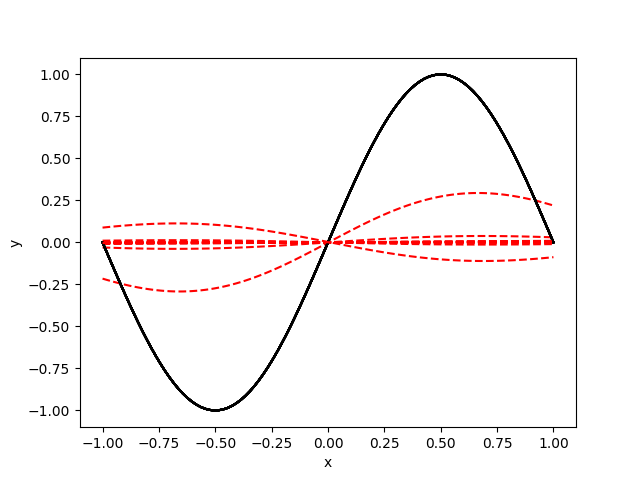
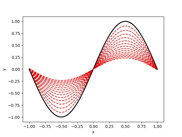
Figure 1: Explicit time discrete training. Left: time step $0.4:$ the approximate solution seems that diverge. Right: time step $0.01:$ with much smaller time step the approximate solution has stable behaviour.

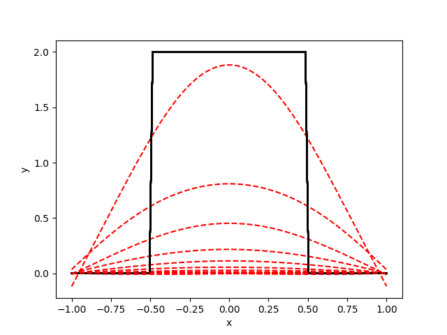
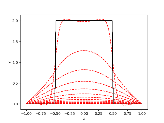
Figure 2: The approximations at times $t_{n}=n(0.2)$, $n=1,2,\dots,$ are displayed with red and the initial condition with black. Left: Explicit time discrete training with time step $0.2$ and $16$ training points. The approximate solution seems that diverge. Left: Implicit time discrete training with time step $0.2$ and $16$ training points. The approximate solution seems reasonable.

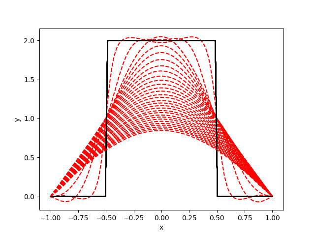
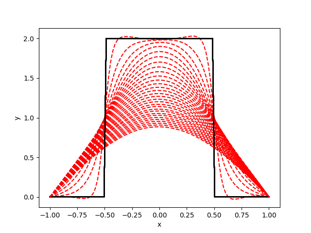
Figure 3: Left: Explicit time discrete training with time step $0.01$ and $16$ training points. The approximate solution seems reasonable due to the much smaller time step. Left: Implicit time discrete training with time step $0.01$ and $16$ training points.

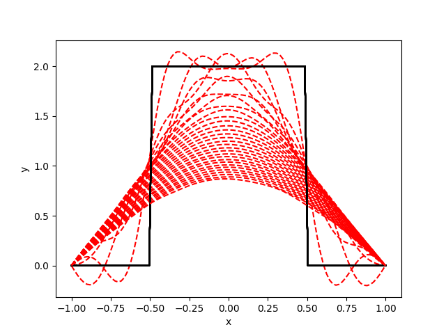
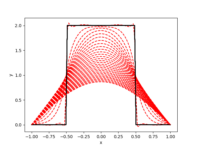
Figure 4: Left: Explicit time discrete training with time step $0.01$ and $100$ training points. Initial instabilities are again evident, due to the higher number of spatial training points while the time step is the same as in Figure 3. Left: Implicit time discrete training with time step $0.01$ and $100$ training points.

Acknowledgments

We would like to thank G. Akrivis, E. Georgoulis, G. Karniadakis, T. Katsaounis, K. Koumatos, M. Loulakis, P. Rosakis, A. Tzavaras and J. Xu for useful discussions and suggestions.

References

• [1] Ahmed Abdeljawad and Philipp Grohs. Approximations with deep neural networks in Sobolev time-space. Anal. Appl., 20(3):499–541, 2022.
• [2] Georgios Akrivis and Charalambos Makridakis. On maximal regularity estimates for discontinuous Galerkin time-discrete methods. SIAM Journal on Numerical Analysis, 60(1):180–194, 2022.
• [3] Genming Bai, Ujjwal Koley, Siddhartha Mishra, and Roberto Molinaro. Physics informed neural networks (PINNs) for approximating nonlinear dispersive PDEs. J. Comput. Math., 39(6):816–847, 2021.
• [4] C. Baiocchi and F. Brezzi. Optimal error estimates for linear parabolic problems under minimal regularity assumptions. Calcolo, 20(2):143–176, 1983.
• [5] Sören Bartels, Andrea Bonito, and Ricardo H Nochetto. Bilayer plates: Model reduction, $\Gamma$-convergent finite element approximation, and discrete gradient flow. Communications on Pure and Applied Mathematics, 70(3):547–589, 2017.
• [6] Jens Berg and Kaj Nyström. A unified deep artificial neural network approach to partial differential equations in complex geometries. Neurocomputing, 317:28–41, nov 2018.
• [7] Julius Berner, Philipp Grohs, Gitta Kutyniok, and Philipp Petersen. The modern mathematics of deep learning. In Mathematical aspects of deep learning, pages 1–111. Cambridge Univ. Press, Cambridge, 2023.
• [8] Stefano Berrone, Claudio Canuto, and Moreno Pintore. Variational physics informed neural networks: the role of quadratures and test functions. J. Sci. Comput., 92(3):Paper No. 100, 27, 2022.
• [9] Andrea Bonito, Ricardo H. Nochetto, and Dimitrios Ntogkas. DG approach to large bending plate deformations with isometry constraint. Math. Models Methods Appl. Sci., 31(1):133–175, 2021.
• [10] Andrea Braides. Gamma-convergence for Beginners, volume 22. Clarendon Press, 2002.
• [11] Haim Brezis. Functional analysis, Sobolev spaces and partial differential equations. Springer Science & Business Media, 2010.
• [12] Xiaoli Chen, Phoebus Rosakis, Zhizhang Wu, and Zhiwen Zhang. A deep learning approach to nonconvex energy minimization for martensitic phase transitions. arXiv preprint 2206.13937, 2022.
• [13] Wolfgang Dahmen, Ronald A. DeVore, and Philipp Grohs. CA special issue on neural network approximation. Constr. Approx., 55(1):1–2, 2022.
• [14] Ennio De Giorgi. Selected papers. Springer Collected Works in Mathematics. Springer, Heidelberg, 2013. [Author name on title page: Ennio Giorgi], Edited by Luigi Ambrosio, Gianni Dal Maso, Marco Forti, Mario Miranda and Sergio Spagnolo, Reprint of the 2006 edition [MR2229237].
• [15] Tim De Ryck, Samuel Lanthaler, and Siddhartha Mishra. On the approximation of functions by tanh neural networks. Neural Networks, 143:732–750, 2021.
• [16] Tim De Ryck, Siddhartha Mishra, and Deep Ray. On the approximation of rough functions with deep neural networks. SeMA J., 79(3):399–440, 2022.
• [17] Sophia Demoulini, David M. A. Stuart, and Athanasios E. Tzavaras. A variational approximation scheme for three-dimensional elastodynamics with polyconvex energy. Arch. Ration. Mech. Anal., 157(4):325–344, 2001.
• [18] Weinan E and Bing Yu. The deep Ritz method: a deep learning-based numerical algorithm for solving variational problems. Communications in Mathematics and Statistics, 6(1):1–12, 2018.
• [19] L. C. Evans. Partial Differential Equations. Graduate Studies in Mathematics 19. American Mathematical Society, Providence, RI,, 2010.
• [20] Emmanuil H Georgoulis, Michail Loulakis, and Asterios Tsiourvas. Discrete gradient flow approximations of high dimensional evolution partial differential equations via deep neural networks. Communications in Nonlinear Science and Numerical Simulation, 117:106893, 2023.
• [21] Georgios Grekas. Modelling, Analysis and Computation of Cell-Induced Phase Transitions in Fibrous Biomaterials. PhD thesis, University of Crete, 2019.
• [22] Georgios Grekas, Konstantinos Koumatos, Charalambos Makridakis, and Phoebus Rosakis. Approximations of energy minimization in cell-induced phase transitions of fibrous biomaterials: $\Gamma$-convergence analysis. SIAM Journal on Numerical Analysis, 60(2):715–750, 2022.
• [23] Philipp Grohs, Fabian Hornung, Arnulf Jentzen, and Philipp Zimmermann. Space-time error estimates for deep neural network approximations for differential equations. Adv. Comput. Math., 49(1):Paper No. 4, 78, 2023.
• [24] Lukas Herrmann, Joost A. A. Opschoor, and Christoph Schwab. Constructive deep ReLU neural network approximation. J. Sci. Comput., 90(2):Paper No. 75, 37, 2022.
• [25] Qingguo Hong, Jonathan W. Siegel, and Jinchao Xu. A priori analysis of stable neural network solutions to numerical pdes, 2022.
• [26] George Em Karniadakis, Ioannis G Kevrekidis, Lu Lu, Paris Perdikaris, Sifan Wang, and Liu Yang. Physics-informed machine learning. Nature Reviews Physics, 3(6):422–440, 2021.
• [27] E. Kharazmi, Z. Zhang, and G. E. Karniadakis. Variational physics-informed neural networks for solving partial differential equations, 2019.
• [28] Balázs Kovács, Buyang Li, and Christian Lubich. A-stable time discretizations preserve maximal parabolic regularity. SIAM Journal on Numerical Analysis, 54(6):3600–3624, 2016.
• [29] I.E. Lagaris, A. Likas, and D.I. Fotiadis. Artificial neural networks for solving ordinary and partial differential equations. IEEE Transactions on Neural Networks, 9(5):987–1000, 1998.
• [30] P. D. Lax and R. D. Richtmyer. Survey of the stability of linear finite difference equations. Comm. Pure Appl. Math., 9:267–293, 1956.
• [31] Dmitriy Leykekhman and Boris Vexler. Discrete maximal parabolic regularity for Galerkin finite element methods. Numerische Mathematik, 135(3):923–952, 2017.
• [32] Michail Loulakis and Charalambos G. Makridakis. A new approach to generalisation error of machine learning algorithms: Estimates and convergence. arXiv preprint 2306.13784, 2023.
• [33] Lu Lu, Xuhui Meng, Zhiping Mao, and George Em Karniadakis. DeepXDE: a deep learning library for solving differential equations. SIAM Rev., 63(1):208–228, 2021.
• [34] Charalambos Makridakis and Ricardo H Nochetto. A posteriori error analysis for higher order dissipative methods for evolution problems. Numerische Mathematik, 104(4):489–514, 2006.
• [35] Siddhartha Mishra and Roberto Molinaro. Estimates on the generalization error of physics-informed neural networks for approximating a class of inverse problems for PDEs. IMA J. Numer. Anal., 42(2):981–1022, 2022.
• [36] Siddhartha Mishra and Roberto Molinaro. Estimates on the generalization error of physics-informed neural networks for approximating PDEs. IMA J. Numer. Anal., 43(1):1–43, 2023.
• [37] Johannes Müller and Marius Zeinhofer. Deep Ritz revisited. arXiv preprint arXiv:1912.03937, 2019.
• [38] Ricardo H Nochetto, Giuseppe Savaré, and Claudio Verdi. A posteriori error estimates for variable time-step discretizations of nonlinear evolution equations. Communications on Pure and Applied Mathematics, 53(5):525–589, 2000.
• [39] M. Raissi, P. Perdikaris, and G. E. Karniadakis. Physics-informed neural networks: a deep learning framework for solving forward and inverse problems involving nonlinear partial differential equations. J. Comput. Phys., 378:686–707, 2019.
• [40] Maziar Raissi and George Em Karniadakis. Hidden physics models: Machine learning of nonlinear partial differential equations. Journal of Computational Physics, 357:125–141, mar 2018.
• [41] Ramiro Rico-Martinez, K Krischer, IG Kevrekidis, MC Kube, and JL Hudson. Discrete-vs. continuous-time nonlinear signal processing of cu electrodissolution data. Chemical Engineering Communications, 118(1):25–48, 1992.
• [42] Sandro Salsa. Partial differential equations in action: from modelling to theory, volume 99. Springer, 2016.
• [43] Christoph Schwab and Jakob Zech. Deep learning in high dimension: neural network expression rates for analytic functions in $L^{2}(\mathbb{R}^{d},\gamma_{d})$. SIAM/ASA J. Uncertain. Quantif., 11(1):199–234, 2023.
• [44] Yeonjong Shin, Jérôme Darbon, and George Em Karniadakis. On the convergence of physics informed neural networks for linear second-order elliptic and parabolic type PDEs. Commun. Comput. Phys., 28(5):2042–2074, 2020.
• [45] Yeonjong Shin, Zhongqiang Zhang, and George Em Karniadakis. Error estimates of residual minimization using neural networks for linear pdes. arXiv preprint 2010.08019, 2020.
• [46] Justin Sirignano and Konstantinos Spiliopoulos. DGM: a deep learning algorithm for solving partial differential equations. J. Comput. Phys., 375:1339–1364, 2018.
• [47] N Sukumar and Ankit Srivastava. Exact imposition of boundary conditions with distance functions in physics-informed deep neural networks. Computer Methods in Applied Mechanics and Engineering, 389:114333, 2022.
• [48] Jinchao Xu. Finite neuron method and convergence analysis. Commun. Comput. Phys., 28(5):1707–1745, 2020.
• [49] S. Zheng. Nonlinear Evolution Equations. 1st Edition, Chapman and Hall/CRC, 2004.