Guided quantum walk

Abstract

We utilize the theory of local amplitude transfers (LAT) to gain insights into quantum walks (QWs) and quantum annealing (QA) beyond the adiabatic theorem. By representing the eigenspace of the problem Hamiltonian as a hypercube graph, we demonstrate that probability amplitude traverses the search space through a series of local Rabi oscillations. We argue that the amplitude movement can be systematically guided towards the ground state using a time-dependent hopping rate based solely on the problem’s energy spectrum. Building upon these insights, we extend the concept of multi-stage QW by introducing the guided quantum walk (GQW) as a bridge between QW-like and QA-like procedures. We assess the performance of the GQW on exact cover, traveling salesperson and garden optimization problems with 9 to 30 qubits. Our results provide evidence for the existence of optimal annealing schedules, beyond the requirement of adiabatic time evolutions. These schedules might be capable of solving large-scale combinatorial optimization problems within evolution times that scale linearly in the problem size.

I Introduction

Combinatorial optimization is a fundamental problem in computer science that has a wide range of important applications in finance [1], scheduling [2], machine learning [3, 4], database search [5], computational biology [6], and operations research [7]. However, finding optimal solutions to such problems can be challenging and computationally expensive, which often makes them intractable for classical computers today. Recent advances in quantum hardware are raising the expectations for demonstrating useful quantum computation in the upcoming years. In particular, solving large-scale combinatorial optimization problems is considered one of the great application areas of quantum computation, driving the need for quantum optimization algorithms suitable for near-term quantum devices [8].

Quantum walks (QW) [9, 10, 5, 11, 12] and quantum annealing (QA) [13, 14, 15, 16, 17, 18, 19, 20, 21, 22] have emerged as two promising candidates for continuous-time quantum optimization algorithms in this context. QWs, introduced by Aharonov et al. [9], model the search space as a graph and govern the walker’s transitions between vertices using a time-independent Hamiltonian. On the other hand, QA employs a time-dependent Hamiltonian to adiabatically evolve from an initial Hamiltonian to a problem Hamiltonian. Both algorithms have been extensively studied for various problems with tens of qubits, including Sherrington-Kirkpatrick spin glasses [23, 11], Max-Cut [12], 2-SAT [24, 25, 26, 27, 28] and exact cover [2] problem instances. While these algorithms exhibit distinct dynamics, Morley et al. [29] have argued that they can be seen as extreme cases of annealing schedules in the context of search problems. However, the dynamics occurring in the intermediate region between QA and QW for combinatorial optimization problems have yet to be fully explored. We argue that these intermediate evolutions, which go beyond the scope of the adiabatic theorem, are a very promising regime for effective quantum computation.

In this paper, we utilize the theory of local amplitude transfers (LAT) to investigate continuous-time quantum algorithms. LAT theory focuses on the local energy structure of the problem Hamiltonian on the hypercube graph. It provides insights into the movement of probability amplitude between individual elements of the search space through a series of local Rabi oscillations.

Building upon these insights, we extend the concept of multi-stage QW [11, 12] by introducing the guided quantum walk (GQW). The GQW combines multiple QWs through a time-dependent hopping rate, effectively guiding the transfer of probability amplitude throughout the graph. This approach relates to the problem of finding optimal annealing schedules [30, 31, 32], but goes beyond the requirement of adiabatic time evolutions, placing the GQW in between QW-like and QA-like procedures.

To evaluate the performance of the GQW, we numerically simulate its application to exact cover (EC) [33, 34, 2], traveling salesperson (TSP) [35, 36, 37, 7, 38], and garden optimization (GO) [39] problems using the JUWELS Booster supercomputer [40]. We extensively study the GQW on problem instances with up to 30 qubits. Our results provide evidence for the existence of optimal annealing schedules capable of solving large-scale combinatorial optimization problems with evolution times that scale linearly in the problem size.

The paper is organized as follows: In Sec. II, we introduce the types of combinatorial optimization problems that are used in our research. Section III provides a review of QWs and explores their dynamics on search and optimization problems using the LAT theory. We discuss how probability amplitude can be effectively guided through the hypercube graph, leading to the development of the GQW. Furthermore, we examine the relationship between the GQW, QA and QWs at different evolution times. In Sec. IV, we present a comprehensive performance analysis of the GQW. Finally, in Sec. V, we summarize our findings and their implications for future research.

II Combinatorial Optimization Problems

This section presents the combinatorial optimization problems studied in our research. First, we describe the problem types and their encoding into a quantum setting in Sec. II.1. Subsequently, we introduce a benchmarking metric, the solution quality, which ensures fair comparisons of quantum optimization algorithms across different problem types and sizes in Sec. II.2.

II.1 Definition

A broad class of real-world problems can be framed as combinatorial optimization problems [7]. These are problems defined on N-bit binary strings $z=z_{N-1}\dots z_{0}=\left\{0,1\right\}^{\otimes N}$, with the objective of finding a string $z_{opt}$ that minimizes a given classical cost function $C\left(z\right):\left\{0,1\right\}^{\otimes N}\xrightarrow{}\mathbb{R}_{\geq 0}$. A natural way to express $C$ in a quantum setting is to encode it into the energy spectrum of the computational basis states $\ket{z}$ of a quantum cost Hamiltonian

$$\hat{H}_{C}=\sum_{z\,\in\,\left\{0,1\right\}^{\otimes N}}C\left(z\right)\ket{z}\bra{z}.$$ (1)

We consider the case in which $C\left(z\right)$ consists only of linear and quadratic terms, $C\left(z\right)=\sum_{ij}z_{i}Q_{ij}z_{j}$. Such problems are known as quadratic unconstrained binary optimization (QUBO) problems, with $\{Q_{ij}\}$ denoting the QUBO coefficients. For these problems, $\hat{H}_{C}$ can be written in the form of an Ising Hamiltonian by substituting $z_{i}\mapsto(1-\hat{\sigma}_{i}^{z})/2$, where $\hat{\sigma}_{i}^{z}$ denotes the Pauli-Z operator applied to the ith qubit with the identity operator acting on the remaining qubits. One obtains

$$\hat{H}_{C}=-\sum_{i=0}^{N-1}h_{i}\hat{\sigma}_{i}^{z}+\sum_{i\neq j}J_{ij}\hat{\sigma}_{i}^{z}\hat{\sigma}_{j}^{z},$$ (2)

with the coefficients $h_{i}=\sum_{j}(Q_{ij}+Q_{ji})/2$ and $J_{ij}=Q_{ij}/4$ representing the optimization problem. In our study, we investigate three types of combinatorial optimization problems, which can be expressed in Ising form and represent two categories of cost functions.

The first category (constraint-only) concerns cost functions consisting entirely of constraining terms, meaning that all states describing valid solutions to the optimization problem (called valid states henceforth) are assigned to the same cost value. Here, we focus on EC problem instances with $N\in\left\{12,15,18,21,24,30\right\}$. Generically, these problem instances exhibit numerous distinct energy levels with low degeneracies and a non-degenerate ground state.

The second category (constraint+optimization) includes cost functions that involve both constraining and optimization terms, such that the set of valid states spans multiple energy levels. We consider TSP and GO problem instances with $N\in\left\{9,16,25\right\}$ and $N\in\left\{12,15,18,21,24,30\right\}$, respectively. It is worth noting that the GO instances generally exhibit higher degeneracies among their energy levels compared to the TSP instances.

The explicit cost functions for the three types of combinatorial optimization problems can be found in App. A. For each problem type and size, we investigate $10$ randomly generated problem instances. Note that all cost functions have been rescaled and shifted, such that $C\left(z_{opt}\right)=0$ and $\max_{z}C\left(z\right)=100$.

II.2 Solution quality

Quantum optimization algorithms are designed to find the optimal solution to a given combinatorial optimization problem (Eq. (1)) with high success probability $P_{gs}=P_{z_{opt}}=\left|\braket{z_{opt}}{\Psi}\right|^{2}$, where $\ket{\Psi}=\sum_{z}\psi_{z}\ket{z}$ denotes the final quantum state. However, in many cases, approximate solutions, where not solely the solution state but also other valid states with a slightly larger cost function value are obtained with high probability, are also of interest, especially if they can be found significantly faster. Since $P_{gs}$ does not take these approximate solutions into account, a common approach is to evaluate the performance of quantum optimization algorithms based on the energy expectation value

$$E_{\Psi}=\braket{\Psi}{\hat{H}_{C}}{\Psi},$$ (3)

often in the form of the approximation ratio $r\left(\Psi\right)=E_{\Psi}/E_{max}$, where $E_{max}=\max_{z}E_{z}$. Note that smaller approximation ratios are supposed to represent better solutions. However, $r$ is often not able to capture the ’quality’ of the produced quantum state $\ket{\Psi}$, that is the distribution of the measurement probabilities w.r.t. the energies of the valid states. This is because $r$ considers not only the set of valid states (which we are generally interested in) but also the set of invalid states (i.e. states that violate at least one constraint and may shift $E_{max}$ arbitrarily). For the problems under investigation, the latter correspond to the majority of states, covering $\geq 95\%$ of the total energy range. Hence, comparing the approximation ratio between different quantum optimization algorithms does not necessarily compare their ability to produce ’good’ approximate solutions, as a final state with a large value of $r$ might still provide valid states near the optimal solution with higher probability than a different state of smaller $r$ value.

In order to address this issue, we propose the use of a theoretical benchmarking metric termed the solution quality

$$S_{q}=\sum_{z\,\in\,\text{valid states}}\left[1-r_{valid}\left(z\right)\right]\cdot P_{z},$$ (4)

where $P_{z}=\lvert\braket{\Psi}{z}\rvert^{2}$ represents the measurement probability of the state $\ket{z}$, and $r_{valid}\left(z\right)=E_{z}/\max_{k\,\in\,\text{valid states}}(E_{k})$ is used to give a weight among all valid states in the energy spectrum (note that $\ket{z_{opt}}$ is at $E_{z_{opt}}=0$ by definition). $S_{q}$ is designed to capture both the characteristics of the success probability and the approximation ratio, restricted to the set of valid states. This provides a theoretical benchmarking metric that is comparable across different problem instances by focussing on the practicality of the solutions obtained. Note that $S_{q}\in\left[0,1\right]$, with $S_{q}=1$ corresponding to the solution state $\ket{\Psi}=\ket{z_{opt}}$, and $S_{q}=0$ indicates a final state $\ket{\Psi}$ that consists solely of invalid states and highest-energy valid states with $r_{valid}=1$. The latter are effectively excluded from increasing the solution quality $S_{q}$, because obtaining any valid solution to the constraint+optimization problems (TSP and GO) can be done in polynomial time. Hence, we do not consider an information gain from these states. Furthermore, in the case of constraint-only problem instances (EC), we set $r_{valid}\left(z\right)=0$, such that $S_{q}=P_{gs}$.

III Continuous-time quantum walk

In this section, we provide a concise review of the continuous-time QW (Sec. III.1) and investigate its dynamics on search (Sec. III.2) and combinatorial optimization problems (Sec. III.3) using LAT theory. Our analysis shows that the QW can be systematically guided on the hypercube graph based on the energy spectrum of the problem Hamiltonian. Building upon these insights, we introduce the GQW in Sec. III.4. In Sec. III.5 we examine the relationship between the GQW, QA and QWs.

III.1 Definition

The continuous-time QW is a quantum algorithm that assigns the computational basis states $\ket{j}$ of an $N$-qubit Hilbert space to the set of vertex labels $V=\left\{j\right\}_{j=0}^{2^{N}-1}$ of an undirected graph $G\left(V,T\right)$. In this framework, the vertices encode the walker’s position, and the set of edges $T$ indicate allowed transitions between label pairs $\left(j,k\right)$. The latter is described through an adjacency matrix $A$, whose elements satisfy $A_{j,k}=1$ if an edge in $G$ connects vertices $j$ and $k$, and $A_{j,k}=0$ otherwise. As $G$ is undirected, $A$ is symmetric and can be used to define the quantum-walk Hamiltonian, given by:

$$\hat{H}_{QW}=\Gamma\cdot\hat{H}_{D}=-\Gamma\cdot\sum_{j,k}A_{j,k}\ket{j}\bra{k},$$ (5)

where $\hat{H}_{D}$ denotes the driver Hamiltonian, and $\Gamma$ is the hopping rate. It is important to note that Eq. (5) is not the only possible Hamiltonian for a QW. In the literature, the Laplacian $\hat{L}=-\hat{H}_{D}-\hat{D}$ of $G$ is often used instead of $\hat{H}_{D}$, with the diagonal matrix $\hat{D}=\sum_{j}\text{deg}(j)\ket{j}\bra{j}$ encoding the degree $\text{deg}(j)$ of each vertex $j$, i.e. the number of edges incident to $j$ [5]. However, for the regular graphs $G$ considered in this paper, where $\text{deg}(j)$ is constant with respect to $j$, both formulations are equivalent up to an unobservable global phase factor. We chose to use the adjacency operator form of $\hat{H}_{QW}$ for consistency with other quantum optimization algorithms.

Given the QW Hamiltonian (Eq. (5)), the state of the walker evolves from some initial state $\ket{\Psi_{0}}$ according to the time-dependent Schrödinger equation, which yields the state of the system at a time $T$ as

$$\ket{\Psi\left(T\right)}=e^{-i\hat{H}_{QW}T}\ket{\Psi_{0}},$$ (6)

where we have used units with $\hbar=1$. The quantum dynamics implemented by this evolution clearly depend on the connectivity in the graph $G$. In the past, QWs have been studied on a variety of graph layouts, including the complete graph, which couples every vertex to every other, and the $N$-dimensional hypercube, which connects only vertices of Hamming distance one [5]. In this work, we focus on a hypercube, as it provides a natural encoding for a QW into qubits. Specifically, transitioning from one vertex to a neighboring vertex corresponds to flipping the computational state of one qubit. As such, the driving Hamiltonian $\hat{H}_{D}$ is composed of $N$ single-body terms,

$$\hat{H}_{D}=-\sum_{j=1}^{N}\hat{\sigma}_{j}^{x},$$ (7)

where $\hat{\sigma}_{j}^{x}$ denotes the Pauli-X operator applied to the jth qubit with the identity operator acting on the remaining qubits. The corresponding QW Hamiltonian for the hypercube is given by $\hat{H}_{QW}=-\Gamma\cdot\sum_{j=1}^{N}\hat{\sigma}_{j}^{x}$. A primary feature of this Hamiltonian is its ability to rapidly explore the vertices in the graph $G$, thereby providing high dynamics in the computational basis. By introducing a secondary problem Hamiltonian that is diagonal in the computational basis, the graph $G$ becomes directed, leading to a concentration of amplitude in the ground state of the problem Hamiltonian. In the following sections, we investigate this ability of QWs to find ground states, starting with the search problem—a well-studied toy problem that can be analytically solved using the QW.

III.2 Quantum walk search

In the search problem, we aim to find a specific bit string $z_{opt}\in\left\{0,1\right\}^{N}$ from a set of $2^{N}$ possible strings. The problem can be mapped to a quantum setting using an oracle Hamiltonian

$$\hat{H}_{O}=-\ket{z_{opt}}\bra{z_{opt}}$$ (8)

that assigns one unit of energy less to the solution state $\ket{z_{opt}}$ compared to the rest of basis states. Solving the search problem is then equivalent to finding the ground state of $\hat{H}_{O}$. The QW provides a means of solving the search problem by combining $\hat{H}_{O}$ with the driving Hamiltonian $\hat{H}_{D}$ (Eq. (7)), and adjusting their relative strength via the dimensionless hopping rate $\Gamma$. The computation is performed by evolving the quantum system, initialized in the equal superposition state

$$\ket{\Psi_{0}}=\ket{+}^{\otimes N}=\frac{1}{\sqrt{2^{N}}}\sum_{j=0}^{2^{N}}\,\ket{j},$$ (9)

under the QW search Hamiltonian

$$\hat{H}_{QWS}=\Gamma\cdot\hat{H}_{D}+\hat{H}_{O}$$ (10)

for a time $T$ and measuring the qubit register in the computational basis afterward.

Childs and Goldstone have solved the QW search problem analytically for various graph layouts [5], including the complete and hypercube graphs. For each layout, they have calculated optimal values $\Gamma=\Gamma_{opt}$ (see also [10]) for which the performance of the QW search achieves the same optimal quadratic speed up as Grover’s search algorithm [41].

Figure 1: Application of the QW to solve the search problem for $N=12$ qubits using the Hamiltonian $\hat{H}_{QWS}$ in Eq. (10). (a) Energy spectrum of $\hat{H}_{QWS}$ as a function of the hopping rate $\Gamma$. The blue and red curve denote the ground and first exited state, respectively. The data is shifted by the ground state energy. (b) Overlaps of the ground state (blue) and the first exited state (red) with the solution state (solid) and the initial state (dashed) as a function of $\Gamma$. (c) Solution quality $S_{q}$ as a function of the evolution time $T$ for $\Gamma=\Gamma_{opt}=1/2^{N}\sum_{r=1}^{N}\binom{N}{r}/2r$ [5] (solid blue), $\Gamma=95\%\cdot\Gamma_{opt}$ (dashed red) and $\Gamma=90\%\cdot\Gamma_{opt}$ (dash-dotted green).

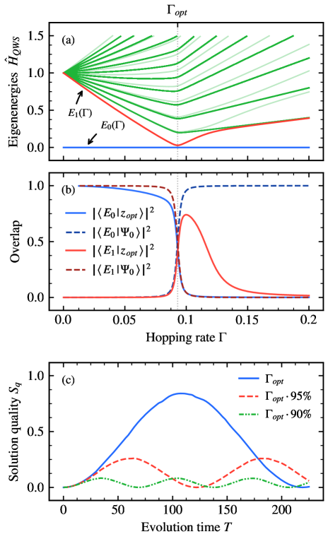
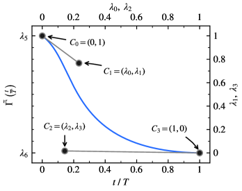
Although the QW search is not applicable in practical situations, because the solution state $\ket{z_{opt}}$ must be known to construct $\hat{H}_{O}$ in the first place, it provides insights into the fundamental characteristics of the QW’s dynamics. Specifically, the entire system evolves periodically, with the individual measurement probabilities of the vertices oscillating as a function of the evolution time $T$. This behavior occurs because the QW performs Rabi oscillations between the initial state $\ket{\Psi_{0}}$ and the solution state $\ket{z_{opt}}$. Figure 1a shows the two lowest energy levels corresponding to the states $\ket{E_{0}(\Gamma)}$ and $\ket{E_{1}(\Gamma)}$ as a function of the hopping rate $\Gamma$. When $\Gamma=\Gamma_{opt}$, the relative strengths of the two contributing Hamiltonians in $\hat{H}_{QWS}$ are balanced equally, and the two energy levels undergo an avoided level crossing. If $N$ is large enough, $\ket{E_{0,1}(\Gamma_{opt})}$ is approximately equal to the uniform superposition of the initial and the solution state, i.e. $\ket{E_{0,1}(\Gamma_{opt})}\approx\left(\ket{\Psi_{0}}\pm\ket{z_{opt}}\right)/\sqrt{2}$ (see Fig. 1b). Hence, $\hat{H}_{QWS}$ drives transitions between $\ket{\Psi_{0}}$ and $\ket{z_{opt}}$ with a frequency $\propto\left[E_{1}(\Gamma_{opt})-E_{0}(\Gamma_{opt})\right]$. Consequently, the overlap with the solution state $|\braket{z_{opt}}{\Psi\left(T\right)}|$ depends on the hopping rate $\Gamma$ and the evolution time $T$, which both require high precision in order to obtain accurate results (see. Fig. 1c).

III.3 Guiding a quantum walk

Combinatorial optimization problems can benefit from the application of QWs, unlike the search problem discussed in the previous section. We can address optimization problems within the QW by augmenting the driver Hamiltonian $\hat{H}_{D}$ with the cost Hamiltonian $\hat{H}_{C}$ defined in Eq. (1). The latter induces complex phase gradients between connected vertices based on their assigned cost value, thereby defining a direction of propagation for the walker in the graph. The QW optimization Hamiltonian on the hypercube mapping is given by

$$\hat{H}_{QWO}=\Gamma\cdot\hat{H}_{D}+\hat{H}_{C},$$ (11)

with $\Gamma$ balancing the relative strength of the two contributing parts. The QW is performed analogously to Sec. III.2, by initializing the qubits in the equal superposition state $\ket{\Psi_{0}}$ (see Eq. (9)), evolving the system under $\hat{H}_{QWO}$ for a time $T$, and then measuring it in the computational basis.

Figure 2: Application of the QW to solve an EC problem for $N=12$ qubits using the Hamiltonian $\hat{H}_{QWO}$ in Eq. (11). (a) Energy spectrum of $\hat{H}_{QWO}$ as a function of the hopping rate $\Gamma$. The blue and red curve denote the ground and first exited state, respectively. The data is shifted by the ground state energy. (b) Overlaps of the ground state (blue) and the first exited state (red) with the solution state (solid) and the initial state (dashed) as a function of $\Gamma$. (c) Solution quality $S_{q}$ as a function of the evolution time $T$ for $\Gamma=\Gamma_{opt}$ (solid blue), $\Gamma=1.2\cdot\Gamma_{opt}$ (dashed red) and $\Gamma=1.5\cdot\Gamma_{opt}$ (dash-dotted green). The value of $\Gamma_{opt}$ has been computed numerically.

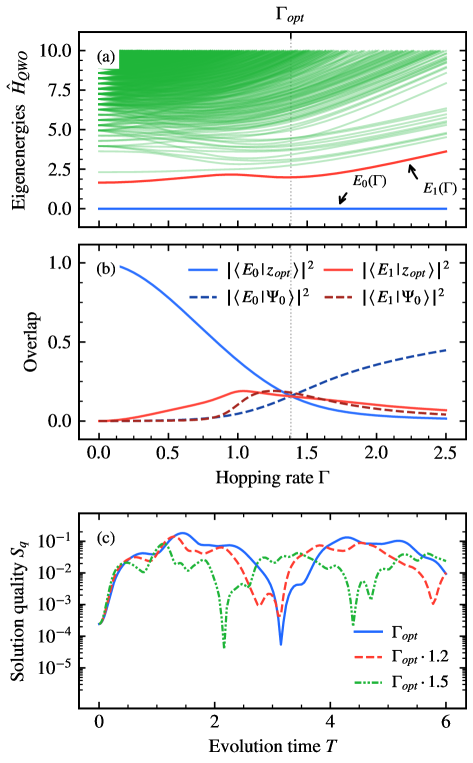
However, unlike for the search problem, the evolution under $\hat{H}_{QWO}$ cannot be efficiently calculated analytically. This makes it impractical to predict optimal parameter sets $\Gamma_{opt}$ and $T_{opt}$ which maximize the final overlap with the solution state for an arbitrary optimization problem. This is because the energy spectrum of $\hat{H}_{C}$ typically features numerous distinct levels with unknown energy gaps, in contrast to the almost completely degenerate spectrum of $\hat{H}_{O}$. Consequently, the energy levels of the combined Hamiltonian split as a function of $\Gamma$ and thereby undergo numerous avoided level crossings (see Fig. 2a). Since the system is initialized in a superposition across multiple energy levels, $\hat{H}_{QWO}$ drives transitions between various eigenstates, so the simple two-level description of the walker’s dynamics used previously is no longer applicable (see Fig. 2b). As a result, the oscillation of the solution quality $S_{q}$ becomes highly complex, as multiple streams of amplitude transfers at different energy levels interfere with each other (see Fig. 2c).

Previous studies have explored heuristic approaches to obtain near-optimal hopping rates $\Gamma$ for the QW within polynomial time. For instance, Callison et al. proposed estimating $\Gamma_{opt}$ from the overall energy scale of $\hat{H}_{C}$ by matching the total energy spreads of the two Hamiltonians in $\hat{H}_{QWO}$ [23]. Later, the authors extended this strategy by sampling $\Gamma_{opt}$ based on a maximization of the average dynamics on Sherrington–Kirkpatrick spin glass problems [11]. Recently, Banks et al. investigated the link between time-independent Hamiltonians and thermalization, leading to an estimate of $\Gamma_{opt}$ through the Eigenstate Thermalization Hypothesis on Max-Cut problem instances [12].

While these strategies demonstrate the general ability of QWs to solve combinatorial optimization problems, they necessitate additional adjustments for each problem type (e.g., estimating energy gaps) and focus solely on the average dynamics in the hypercube graph. However, local variations in these dynamics across different regions of the graph are the primary reason for the observed distortions in the oscillation of the solution quality in Fig. 2c. These distortions not only make it challenging to estimate $T_{\text{opt}}$ from a few samples, but also limit the maximally achievable solution quality for any $T$ as the system approaches a stationary state (cf. Fig. 4 below). The optimal solution quality typically scales exponentially with the problem size $N$ (cf. Fig. 7b below) because the QW can only drive amplitude transfers within a fixed energy range, neglecting the amplitude originating from exponentially many states outside this range. Consequently, the QW as defined in Eq. (11) is not well-suited for large combinatorial optimization problems.

Inspired by these strategies, but being interested in achieving practical quantum computation (as measured by a large solution quality) for any given evolution time $T$, problem size $N$ and problem type, we investigate the dynamics of QWs by applying LAT theory to the hypercube graph $G$ shown in Fig. 3a. By analyzing the transfer of probability amplitude in local subspaces spanned by basis-state pairs with Hamming distance 1 (i.e., states connected by an edge in $G$), we aim to derive a mechanism to control the movement of the walker locally in the graph, such that backpropagation of amplitude into (undesired) high-energy states can be suppressed. Thus, instead of maximizing transitions in the entire graph collectively, as proposed in prior work, our approach is to maximize them only locally at a time in order to guide the walker towards the solution state more effectively.

The LAT theory focuses on two-dimensional subspaces spanned by pairs of basis states, $\ket{j}$ and $\ket{k}$, that are connected in the hypercube graph $G$, i.e. $\braket{j}{\hat{H}_{D}}{k}\neq 0$ (see inset of Fig. 3a). The effective two-level subspace Hamiltonian is given by

$$\hat{H}_{QWO}^{(j,k)}=\Gamma\hat{H}_{D}^{(j,k)}+\hat{H}_{C}^{(j,k)},$$ (12)

assuming the rest of the system remains in its initial state. Here, $\hat{H}_{C}^{(j,k)}$ denotes the local cost Hamiltonian and $\hat{H}_{D}^{(j,k)}$ is the local driving Hamiltonian, which are defined as

$$\hat{H}_{C}^{(j,k)}=\begin{pmatrix}\braket{j}{\hat{H}_{C}}{j}&0\\ 0&\braket{k}{\hat{H}_{C}}{k}\end{pmatrix}\qquad\hat{H}_{D}^{(j,k)}=-\begin{pmatrix}0&1\\ 1&0\end{pmatrix}.$$ (13)

If the system starts in the local equal superposition state, $\ket{+}^{(j,k)}=\left(\ket{j}+\ket{k}\right)/\sqrt{2}$, with the local energy gaps $\Gamma\Delta^{D}=-2\Gamma$ of $\Gamma\hat{H}_{D}^{(j,k)}$ and $E_{j}-E_{k}=\Delta^{C}_{j,k}=2\delta$ of $\hat{H}_{C}^{(j,k)}$, the measurement probability of the desired lower-energy state $\ket{k}$, is given by

$$P_{k}(t,\Gamma)=\frac{1}{2}+\frac{\Gamma\cdot\delta}{\Gamma^{2}+\delta^{2}}\sin\left(\sqrt{\Gamma^{2}+\delta^{2}}\cdot t\right)^{2}.$$ (14)

Equation (14) represents a sinusoidal oscillation with a Rabi frequency of $\omega=\sqrt{\Gamma^{2}+\delta^{2}}$ similar to Sec. III.2 (note that this property holds for any initial state). Specifically, if $\Gamma\gg 1$, the driving Hamiltonian dominates $\hat{H}_{QWO}^{(j,k)}$, and the cost Hamiltonian has almost no influence on the system’s evolution. Since $\ket{+}^{(j,k)}$ corresponds to the ground state of $\hat{H}_{D}^{(j,k)}$, the system remains primarily in its initial state. Conversely, if $\Gamma\ll 1$, $\hat{H}_{C}^{(j,k)}$ governs the evolution. Since $\hat{H}_{C}^{(j,k)}$ is diagonal and only induces phase rotations in the computational basis, no amplitude transfer occurs. Only when $|\Gamma\Delta^{D}|\approx\Delta^{C}_{j,k}/2$, the two Hamiltonians’ relative strengths are balanced, and transitions in the local subspace are maximized.

Figure 3: Energy spectrum analysis of an $N=21$ qubit EC problem. (a) Hypercube graph representation of $\hat{H}_{C}$, where each point corresponds to a computational basis state $\ket{j}$, ordered by increasing energy $E_{j}=\bra{j}\hat{H}_{C}\ket{j}$ from left to right. The color of each point represents the total Hamming distance to the ground state $z_{opt}$. Two states $\ket{j}$ and $\ket{k}$ are connected by an edge if the bitstrings $j$ and $k$ have a Hamming distance of $1$, meaning that the driver Hamiltonian $\hat{H}_{D}$ drives transitions between them. The inset in panel (a) provides a zoomed-in view near $z_{opt}$, highlighting the energy gaps $\Delta^{C}_{j,k}$ between connected states $\ket{j}$ and $\ket{k}$. (b) Distribution of the largest energy gaps $\Delta^{C}_{j,k}$ from a vertex $\ket{j}$ to a lower energy vertex $\ket{k}$ as a function of $E_{j}$. The data reveals an increasing trend of $\Delta^{C}_{j,k}$ with respect to $E_{j}$. The solid black curve represents a fit to the average energy gap $\braket{\Delta^{C}}(E)$ at energy level $E$ (using the scale of the top axis), used by the GQW to locally adjust the relative strength of the driving and problem Hamiltonian in Eq. (11). The dashed black curve illustrates the optimal relative strength for a QW. The bottom axis denotes the relative time in both algorithms, with time progressing from right to left, as the GQW progresses from high-energy to low-energy amplitude transfers.

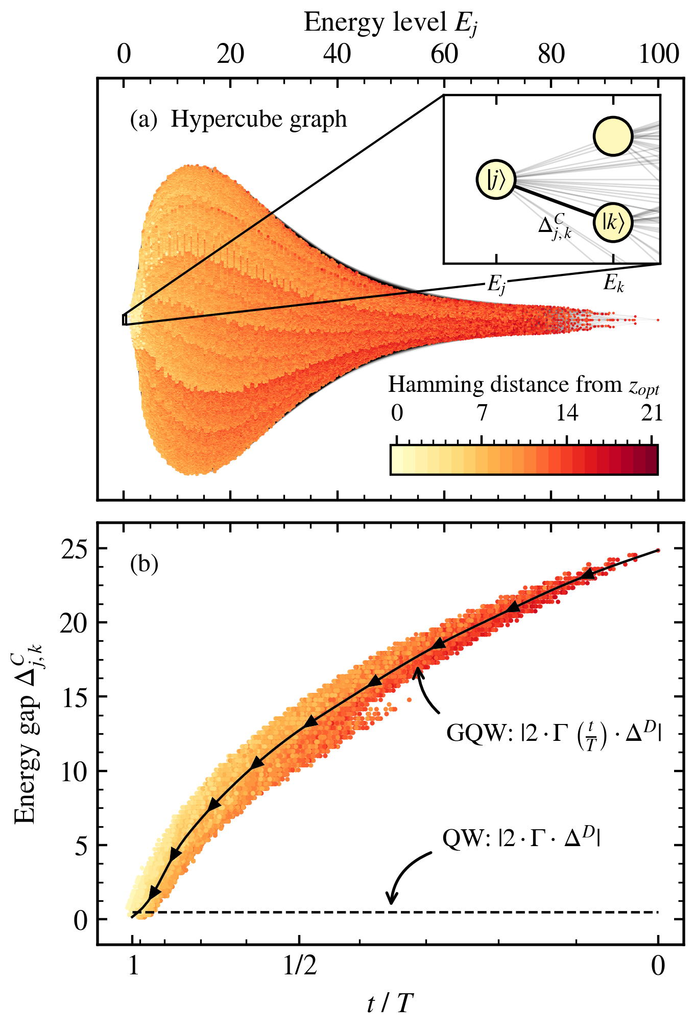
As a result, amplitude transfers can only occur efficiently among specific subsets of vertex pairs with an energy gap $\Delta^{C}_{j,k}\approx|2\Gamma\Delta^{D}|$ in $\hat{H}_{C}$. Transitions between states with significantly larger or smaller energy gaps are suppressed for fixed $\Gamma$. Since the energy gaps of vertex pairs typically vary throughout the graph, we can steer the walker’s movement effectively by selecting $\Gamma$ to activate only the desired transitions in the graph. The primary insight behind this strategy is that, for sufficiently complex problems, the largest energy gap $\Delta^{C}_{j,k}$ from vertex $\ket{j}$ to a lower energy vertex $\ket{k}$ increases approximately monotonically as a function of its energy level $E_{j}$ (see Fig. 3b). Consequently, large values of $\Gamma$ are usually optimal in the regime of high-energy states, while small values are preferable near the solution state. Choosing a fixed value for $\Gamma$ has the disadvantage of limiting the maximally achievable success probability because not all edges can sufficiently contribute to the amplitude transport. In particular, only amplitude transfers within a fixed energy range can be addressed, generally prohibiting states located at high energies from transporting amplitude to the solution state.

The strategy we propose in this paper is based on an energy-dependent hopping rate, where $|2\tilde{\Gamma}(E)\cdot\Delta^{D}|$ corresponds to the average $\braket{\Delta^{C}}\left(E\right)$ of the largest energy gaps of $\hat{H}_{C}$ at energy level $E$ in the graph. The approach is to confine the walker to a gradually shrinking energy region around the solution state by progressing monotonically from high-energy to low-energy optimal hopping rates $\tilde{\Gamma}$. Therefore, we set $\Gamma(t)=\tilde{\Gamma}\left(E\left(t\right)\right)$, where $E\left(t\right)$ is a monotonic sweep, and define

$$\hat{H}_{GQW}=\Gamma(t)\cdot\hat{H}_{D}+\hat{H}_{C}.$$ (15)

Equation 14 shows that the frequency of the local Rabi oscillations is higher at larger energy gaps, which results in fast amplitude transfers at large energies (see Fig. 3b). To compensate for this, we choose the rescaled time

$$s(t)=\frac{\int_{E_{max}+(E_{min}-E_{max})\cdot t/T}^{E_{max}}\braket{\Delta^{C}}(E)\;dE}{\int_{E_{min}}^{E_{max}}\braket{\Delta^{C}}(E)\;dE}$$ (16)

with $E(t)=E_{max}+(E_{min}-E_{max})\cdot s(t)$, where $E_{min}$ and $E_{max}$ denote the lowest and highest energy levels of $\hat{H}_{C}$, respectively, and $T$ is the total evolution time. At $t=0$, the algorithm starts with a relatively high hopping rate ($\Gamma=\tilde{\Gamma}(E_{max})$) that maximizes amplitude transfers only at high energy levels and suppresses dynamics at low and intermediate energies. As the hopping rate is decreased in time, the system starts to perform amplitude transfers at lower energy levels. Simultaneously, subspaces at higher energies become gradually detuned again, suppressing the action of the driving Hamiltonian. This is essential as it prevents the backpropagation of probability into high-energy states and enables us to actively guide the walker towards low-energy states.

The primary advantage of this approach lies in the establishment of a continuous amplitude flow from all computational basis states towards the solution state, consequently overcoming the previous limitation on the maximally achievable solution quality. Furthermore, the latter is no longer subject to the complex interference of multiple amplitude streams in the graph, which requires a precisely chosen evolution time $T$ (cf. Fig. 2c). Instead, $S_{q}(T)$ exhibits the collective sinusoidal oscillation of Eq. (14), where the selection of $\Gamma(t)$ ensures that active subspaces oscillate with similar Rabi frequencies while high energy subspaces become gradually detuned, hence suppressing the backpropagation of probability amplitude. By varying the evolution time $T$, the speed at which $\tilde{\Gamma}(E)$ is swept can be adjusted, thereby altering the duration that groups of subspaces remain active. As a result, $S_{q}(T)$ depends solely on the order of magnitude of $T$, rather than its precise value.

To evaluate the efficiency of a GQW, we compare its performance to a conventional QW on an EC problem instance comprising $N=21$ qubits. Figure 3b shows the average $\braket{\Delta^{C}}(E)$ of the largest energy gaps between connected vertices at each energy level $E$. We obtain $|2\tilde{\Gamma}(E)\cdot\Delta^{D}|$ by fitting a polynomial of degree $6$ to the data points (see the black arrows in Fig. 3b). The bottom axis indicates the non-linear sweep of $E\left(t\right)$. In comparison, for the QW, we determined $\Gamma_{opt}$ by sampling a classical optimizer (see dashed black curve). $\Gamma_{opt}$ corresponds to the optimal hopping rate that yields the highest success probability over $T\in\left[0.1,10.0\right]$.

Figure 4: Performance comparison between the GQW (blue) and the QW (red) on the $N=21$ qubit EC problem depicted in Fig. 3. The GQW dynamically adjusts the relative strength $\Gamma$ of the driving and problem Hamiltonian in Eq. (15) based on the average $\braket{\Delta^{C}}(E)$ of the largest energy gaps in $\hat{H}_{C}$. In contrast, the QW employs a fixed hopping rate $\Gamma$ that has been pre-optimized (see Fig. 3b). The performance is evaluated using the solution quality $S_{q}$, as defined in Eq. (4). Note that the results presented here are indicative and require knowledge of the complete energy spectrum.

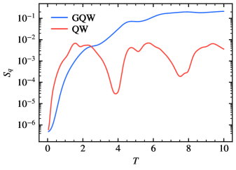
Figure 4 compares the performance of the GQW and the QW as a function of the total evolution time $T$. For $T\leq 2$, both strategies exhibit similar behavior, showing a rapid increase in solution quality, with the QW achieving its peak at $T=1.5$. Notably, for $T\leq 2.5$, the GQW yields lower solution qualities compared to the QW. This discrepancy arises from the relatively small optimal hopping rate of the QW, enabling it to focus its evolution on amplitude transitions near and into the solution state. In contrast, the GQW considers the entire graph and therefore spends the initial part of its evolution at high and intermediate energy levels (the right part of Fig. 3b). This approach leads to very short evolutions at each energy level for small $T$, causing only fractions of the probability amplitudes to be transported towards $z_{opt}$. However, as $T$ increases, the situation changes, and the GQW obtains superior solution qualities to the QW for $T\geq 2.5$. Here, the QW exhibits oscillatory behavior between $10^{-5}$ to $10^{-2}$. In contrast, the GQW follows a monotonic increase without oscillations, where $S_{q}(T)$ saturates at approximately $21\%$, outperforming the QW by approximately one order of magnitude.

This saturation is caused by the concentration of substantial amplitude within a few states towards the end of the evolution. Consequently, significant imbalances occur within the local subspaces at small $E$ (i.e., the system is no longer in a close-to-equal local superposition state), which eventually drive amplitude transfers back into high-energy states.

III.4 Practical guided quantum walk

The previous section has shown the potential of GQWs for solving combinatorial optimization problems, by adjusting the relative strength of the two Hamiltonians in $\hat{H}_{GQW}$ based on the walker’s position in the graph. The main benefits are an increased maximum solution quality and a suppression of complex oscillations in $S_{q}(t)$, providing good results for arbitrary $T$ and $N$.

Of course, obtaining the optimal function $\tilde{\Gamma}\left(E(t)\right)$ is generally not efficiently possible, because it requires knowledge of the entire energy spectrum of $\hat{H}_{C}$. In order to still make use of the promising methodology described above, we propose a variational ansatz, in analogy to other quantum optimization algorithms [42, 43, 44]. The idea is to approximate the optimal distribution $\tilde{\Gamma}\left(E\right)$ by a function $\tilde{\Gamma}\left(E,\boldsymbol{\lambda}\right)$, which is tuned using a set of $M$ hyperparameters $\boldsymbol{\lambda}=\left(\lambda_{1},\dots,\lambda_{M}\right)$. Note that henceforth we consider only linear sweeps of the energy spectrum, i.e. $E\left(t\right)=\left(E_{min}-E_{max}\right)\cdot t/T+E_{max}$, thus encoding the sampling speed in the shape of $\tilde{\Gamma}$. The hope is that as long as $\tilde{\Gamma}\left(E,\boldsymbol{\lambda}\right)$ describes $\tilde{\Gamma}\left(E\right)$ closely enough, similar dynamics to Sec. III.3 can be obtained. In fact, introducing hyperparameters into the algorithm even enables the guided quantum walk to overcome its limitations at small and large $T$. For instance, at small $T$, the GQW can selectively model $\tilde{\Gamma}\left(E\right)$ only up to $E_{C}=E_{C}^{\prime}<E_{max}$, thereby operating solely on a subspace of the entire graph near $\ket{z_{opt}}$. Conversely, at large $T$, the GQW can prevent the transfer of amplitude into higher energy states when operating at small $E$ by compensating the imbalances within the local subspaces through a reduction of the final hopping rate, $\tilde{\Gamma}\left(E=E_{min}\right)$.

The proposed algorithm employs a hybrid quantum-classical ansatz, in which a classical optimizer adjusts a set of hyperparameters based on the measurement outcomes of a quantum device performing the guided quantum walk. As with other quantum optimization algorithms, the quality of the produced walk is evaluated using the energy expectation $E_{\Psi}$ (see Eq. (3)). Note that the number $M$ of hyperparameters is fixed, and we investigate the impact of this optimization phase on the total run time in Sec. IV.3.

We propose a function $\tilde{\Gamma}\left(E,\boldsymbol{\lambda}\right)$ based on cubic Bézier curves. We chose Bézier curves instead of simple polynomials because we expect the optimal hopping rate to be smooth and monotonically decreasing in $E$. Although polynomials can produce such functions for $E\in\left[E_{min},E_{max}\right]$, their parameters are generally hard to tune, as small changes can lead to substantially different functions. In contrast, Bézier curves are much easier to optimize because their general shape can be predetermined. Moreover, the latter varies continuously and sufficiently slowly in its parameters, resulting in a sufficiently smooth search space for $\boldsymbol{\lambda}$. Due to these properties, we strongly encourage their use in other fields of quantum computing, such as optimizing annealing schedules [30, 31, 32] or deriving optimal parameter sets for the quantum approximate optimization algorithm (QAOA) [45, 42, 46, 47, 2].

Cubic Bézier curves are based on Bernstein polynomials and are defined through four control points $C_{i}=\left(x_{i},y_{i}\right)^{T}$ in a two-dimensional plane as

$$x(\tau)=x_{0}\left(1-\tau\right)^{3} +3x_{1}\left(1-\tau\right)^{2}\tau$$

$$+3x_{2}\left(1-\tau\right)\tau^{2}+x_{3}\tau^{3}$$ (17)

$$y(\tau)=y_{0}\left(1-\tau\right)^{3} +3y_{1}\left(1-\tau\right)^{2}\tau$$

$$+3y_{2}\left(1-\tau\right)\tau^{2}+y_{3}\tau^{3}.$$ (18)

By requiring $x_{0}<x_{1},x_{2}<x_{3}$, the curve can be mapped into one dimension, by solving $t=x(\tau)$ for $\tau$ and inserting it into $y(\tau)$. Based on the observations made in Sec. III.3, we set $C_{0}=(0,1)$ and $C_{3}=(1,0)$ to ensure a monotonically decreasing function, leaving $4$ hyperparameters $\lambda_{0,1,2,3}\in\left(0,1\right)$ that control the shape of $\tilde{\Gamma}\left(t,\boldsymbol{\lambda}\right)$ and thus the sweep of $E(t)$, i.e. $C_{1}=\left(\lambda_{0},\lambda_{1}\right)^{T}$ and $C_{2}=\left(\lambda_{2},\lambda_{3}\right)^{T}$. In addition to these, we introduce $2$ hyperparameters, $\lambda_{5}$ and $\lambda_{6}$, that describe the boundary conditions $\tilde{\Gamma}\left(t=0,\boldsymbol{\lambda}\right)=\lambda_{5}$ and $\tilde{\Gamma}\left(t=T,\boldsymbol{\lambda}\right)=\lambda_{6}$. Therefore, $\lambda_{5}$ determines the energy range in which the GQW operates in the graph (see discussion for small $T$) and $\lambda_{6}$ controls the detuning of the local subspaces near the solution state (see discussion for large $T$). Throughout this paper, we consider $\lambda_{5}\left(k_{5}\right)=10^{-3\cdot k_{5}}$ and $\lambda_{6}\left(k_{6}\right)=10^{2\cdot k_{6}}$ with $k_{5},k_{6}\in\left[0,1\right]$. It is important to note, however, that the parameter ranges generally depend on the total energy range of the cost Hamiltonian $\hat{H}_{C}$, which we rescaled for all problem instances to the same maximum value (see Sec. II.1). In Fig. 5 we present an example of $\tilde{\Gamma}\left(t,\boldsymbol{\lambda}\right)$ for the aforementioned EC problem and $T=10$.

Figure 5: Optimal hopping rate $\tilde{\Gamma}\left(t,\boldsymbol{\lambda}\right)$ (blue) for the $N=21$ qubit EC problem shown in Fig. 3, with a total evolution time of $T=10$. The hopping rate is represented by a cubic Bézier curve (see Eq. (18)) and is defined by four control points $C_{0,1,2,3}$, along with the boundary conditions $\tilde{\Gamma}\left(t=0,\boldsymbol{\lambda}\right)=\lambda_{5}$ and $\tilde{\Gamma}\left(t=T,\boldsymbol{\lambda}\right)=\lambda_{6}$. The curve is obtained by optimizing a set of six hyperparameters $\boldsymbol{\lambda}$ using the classical Nelder-Mead optimizer [48, 49], employing $N_{opt}=100$ optimization steps starting from a random initial configuration.

III.5 From quantum walk to quantum annealing

Figure 6: Optimized quantum evolutions performed by the GQW on an $N=15$ qubit EC problem for short ($T=0.5$, (a) and (d)), intermediate ($T=2.0$, (b) and (e)), and long ($T=12$, (c) and (f)) evolution times. Panels (a)–(c) illustrate the average measurement probabilities of the energy levels $E_{C}$ of the problem Hamiltonian $\hat{H}_{C}$. Panels (d)–(f) display the evolution of the instantaneous energy levels $E_{GQW}$ of the combined Hamiltonian $\hat{H}_{GQW}$ (Eq. (15)). The blue and red curves represent the instantaneous ground state and the first excited state, respectively. Dashed lines are included in all panels to indicate the instantaneous energy expectation values of the system with respect to $\hat{H}_{C}$ (panels (a)–(c)) and $\hat{H}_{GQW}$ (panels (d)–(f)). The final solution qualities are $S_{q}=0.7\%$ ($T=0.5$), $S_{q}=13.6\%$ ($T=2.0$), and $S_{q}=91.3\%$ ($T=12.0$).

The LAT theory, used in the derivation of the GQW (see Sec. III.3), offers a new perspective on the working principle of quantum annealing (QA) and its relationship to QWs. QA belongs to the class of continuous-time quantum optimization algorithms that rely on an adiabatic transition from the driver Hamiltonian $\hat{H}_{D}$ (i.e., $\Gamma(0)\rightarrow\infty$) to the problem Hamiltonian $\hat{H}_{C}$ (i.e., $\Gamma(T)=0$) throughout the time evolution. According to the adiabatic theorem of quantum mechanics, if this transition occurs sufficiently slowly, and the system is initially prepared in the ground state of $\hat{H}_{D}$, it will remain in the instantaneous ground state of the combined Hamiltonian $\hat{H}_{GQW}$ in Eq. (15), ultimately reaching the solution state $\ket{z_{opt}}$.

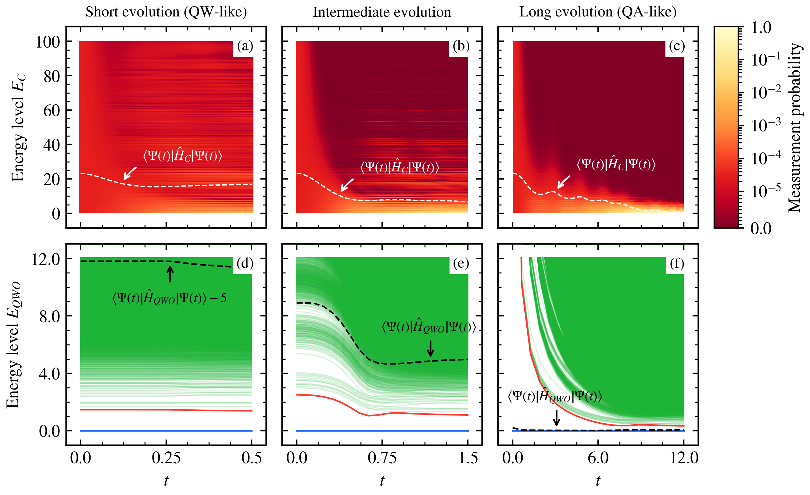
To investigate the relationship between QWs and QA, we use the GQW to examine the strategies underlying optimal quantum evolutions for different evolution times $T$. Figure 6 presents simulation results of the GQW applied to an $N=15$ qubit EC problem for short ($T=0.5$), intermediate ($T=2.0$), and long ($T=12$) evolutions. Panels (a)–(c) illustrate the average measurement probabilities of the energy levels $E$ of the problem Hamiltonian $\hat{H}_{C}$, providing insights into the propagation of probability amplitude through the hypercube graph (cf. Fig. 3a). Panels (d)–(f) display the evolution of the instantaneous energy levels $E_{GQW}$ of the combined Hamiltonian $\hat{H}_{GQW}$. Dashed curves are included to indicate the instantaneous energy expectation value of the system.

Short evolutions:

In the case of short evolutions, the optimal hopping rate schedule $\Gamma(t)$ determined by the GQW maintains a nearly constant relationship between $\hat{H}_{D}$ and $\hat{H}_{C}$ in Eq. (15). Consequently, the instantaneous energy levels mostly remain unchanged during the evolution, and the system starts and ends in a superposition of the instantaneous basis states (see dashed line in Fig. 6d). Due to the relatively small hopping rate, the GQW predominantly drives local subspaces near the solution state (i.e., small $E$, corresponding to the left region of Fig. 3a), resembling a QW-like procedure (see Fig. 3b). Figure 6a demonstrates that this strategy results in a guided movement of amplitude towards $\ket{z_{opt}}$ for $E_{C}\leq 12$, evident from the emerging gradient in the measurement probabilities. Probability amplitude originating from intermediate and high energy levels, on the other hand, fails to reach the solution state and instead becomes trapped at these energies within the graph (see horizontal dark and bright stripes in Fig. 6a). This highlights the inherent limitations of QWs.

Intermediate evolutions:

In the case of intermediate evolution times, the optimal hopping rate schedule operates over a wider range of values, featuring a larger initial detuning compared to short evolutions. As a result, the GQW extends the region of the graph in which amplitude is actively guided through local subspaces. This is evident from the increased final success probability and the gradual transport of amplitude from high to low energy states for $t\leq 0.5$ (see Fig. 6b). The presence of bright stripes at $E_{C}\geq 10$ indicates that the GQW is still operating on a subset of the hypercube graph, causing amplitude from high-energy states to become trapped at intermediate energy levels. This demonstrates that even for intermediate evolution times, it is more advantageous to neglect amplitude at high-energy states and focus on amplitude transfers near the solution state.

Long evolutions:

For long evolutions, the optimal hopping rate schedule determined by the GQW resembles an QA-like schedule by incorporating large initial and final detunings in $\hat{H}_{GQW}$ (i.e., $\lambda_{5}\gg 1$ and $\lambda_{6}\ll 1$). As a result, the system follows the instantaneous ground state of $\hat{H}_{GQW}$ throughout the evolution (see dashed line in Fig. 6f). During this process, the GQW successfully drives amplitude transfers across the entire graph, starting from high energy levels and progressing towards low energies, as indicated by the absence of the horizontal stripes in Fig. 3c. Notably, the confinement of amplitude occurs exponentially with respect to $t$, indicating that the GQW employs a non-linear sweep through the energy spectrum (cf. Eq. (16)). Furthermore, the propagation of amplitude follows a wave-like pattern, as illustrated by the dashed line in Fig. 6c. This wavelike pattern arises due to the confinement of amplitude in a decreasing number of vertices, leading to deviations from the equal superposition states in the local subspaces. This results in a temporary backpropagation of amplitude into higher energy states. Nevertheless, the continuous decrease of the hopping rate $\Gamma(t)$ ensures, on average, the transportation of amplitude into the solution state.

The hopping rate schedules determined by the GQW for various $T$ not only emphasize the close relationship between QWs and QA, but also highlight the existence of optimal quantum evolutions that extend beyond the scopes of these two algorithms. While a QW-like strategy is optimal for short evolutions and a QA-like procedure is preferred for long evolutions, our findings reveal that intermediate values of $T$ necessitate a combination of both strategies to maximize the solution quality.

This observation can be explained through LAT theory (see Sec. III.3), as QWs and QA can be viewed as two distinct formulations of the same underlying concept. Both approaches aim to achieve optimal transfer of probability amplitude within local subspaces of the graph. In the case of QWs, this is achieved by utilizing a constant and small hopping rate $\Gamma$, allowing to focus solely on transfers directly into the solution state during short evolutions. However, this strategy becomes suboptimal for long evolutions where sufficient time is available to guide amplitude at higher energy levels as well. As a result, QA guides amplitude throughout the entire graph by connecting multiple local QWs together using a continuously decreasing hopping rate $\Gamma(t)$. Thus, QWs and QA represent the two extremes of the GQW framework, with one concentrating solely on subspaces around the solution state (i.e., $\lambda_{5}\approx\lambda_{6}\ll 1$) and the other considering the entire graph (i.e., $\lambda_{5}\gg 1$ and $\lambda_{6}\ll 1$, cf. Fig. 5).

The GQW operates in the transition region between these two extremes, striking a balance between the number of guided local subspaces (i.e., the amount of guided amplitude) and the time spent at each energy level (i.e., the amount of amplitude transferred within each local subspace) for a given $T$. As will be discussed in Sec. IV.2, these intermediate evolutions, which surpass the limitations of adiabatic time evolutions, might be capable of effectively solving large-scale optimization problems.

Figure 7: Performance comparison of (a) the GQW, (b) the QW, and (c) QA as a function of the total evolution time $T$ on EC problems with problem sizes $N\in\left\{12,15,18,21,24,30\right\}$ (see legend). The performance is assessed based on the solution quality $S_{q}$ defined in (4). Each problem size $N$ is evaluated using a set of $10$ randomly generated problem instances, and the presented data corresponds to the geometric mean solution qualities (solid curves) along with the geometric standard deviations (shaded areas). Note that the GQW and the QW undergo a prior classical optimization phase. The dotted gray lines indicate horizontal cuts ($S_{q}\in\left\{1\%,10\%,90\%\right\}$), which are detailed in Fig. 8. The inset in panel (a) provides a zoomed-in view of the region corresponding to large evolution times $T$. Additionally, the dashed lines in panel (b) indicate the stationary solution quality that the damped oscillation of $S_{q}(T)$ approaches for the QW at large $T$.

IV Results

In this section, we present a comprehensive performance analysis of the GQW. We compare the solution quality $S_{q}$ both as a function of the evolution time $T$ and the system size $N$ to the conventional QW and linear QA (see Sec. IV.1). Section IV.1 provides scaling results of the three algorithms in the regime of large problem instances (i.e., $N\gg 1$). Our analysis indicates that the GQW achieves significantly higher solution qualities within a linearly growing timespan, rendering it a promising candidate for near-term quantum devices. Finally, in Sec. IV.3 we address the impact of the classical optimization phase on the total run time, demonstrating that the average time-to-solution scales better by a factor of $\approx 2$ ($\approx 4$) compared to linear QA (QW).

IV.1 Comparison of GQW, QW and QA

We assess the effectiveness of the GQW through numerical simulations carried out on the JUWELS Booster supercomputer at the Jülich Supercomputing Centre of the Forschungszentrum Jülich [40]. We compare its performance against a conventional QW and linear QA. Our simulations consider EC and GO instances with problem sizes $N\in\left\{12,15,18,21,24,30\right\}$, as well as TSP instances with $N\in\left\{9,16,25\right\}$ qubits. To demonstrate the generality of our findings, we examine $10$ randomly generated problem instances for each problem type and size. We remark that the energy spectrum of each problem has been obtained classically, providing the total energy range and the individual energies of the valid states for the calculation of $S_{q}$ (see Eq. (4)). Note, however, that this is done only for the purpose of benchmarking, and it is not required to apply the GQW in a practical scenario.

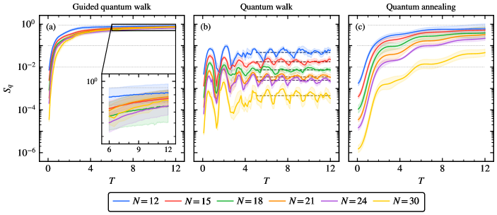
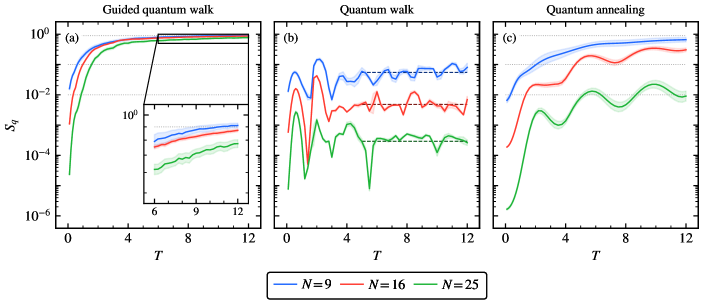
To obtain the final quantum state of the system at the end of each algorithm, we use the second-order Suzuki-Trotter product formula algorithm [50, 51] to solve the time-dependent Schrödinger equation, $i\,\partial t\ket{\Psi(t)}=H(t)\ket{\Psi(t)}$, with a time step of $10^{-5}$ and total evolution times $T$ ranging between $0.1$ and $12.0$, with $0.1$ increments. Given the consistency of our findings, we present the results for the EC instances in Fig. 7, showing the obtained solution qualities averaged within each system size, along with the standard deviations. The analogous results for the TSP and GO problems are available in App. B and support the same conclusions.

Guided quantum walk:

The GQW is adapted to each problem instance and evolution time $T$ individually by tuning its $6$ hyperparameters $\boldsymbol{\lambda}$ to minimize the energy expectation value $E_{\Psi}$ (see Eq. (3)) of the final quantum state $\ket{\Psi}$. Each parameter set is thereby selected from a pool of $N_{rep}=100$ repetitions of the Nelder-Mead classical optimizer, where in each sample the $6$ parameters are initialized randomly and adjusted a maximum of $N_{opt}=100$ times. We choose this approach to ensure that the algorithm converges to a near-optimal minimum in the parameter search space. However, we note that a sufficient set of parameters is typically found within the first $N_{rep}=20$ repetitions. In Sec. IV.3, we discuss the impact of this optimization phase on the total run time.

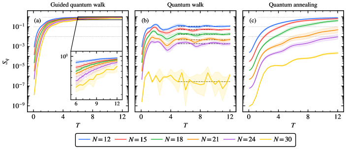
Figure 7a presents the simulation results of the GQW, showing the scaling behavior of the solution quality $S_{q}(T)$ as a function of the evolution time $T$. Across various problem types and sizes, we observe consistent patterns in the scaling of $S_{q}(T)$, which can be categorized into two regions according to Sec. III.5.

For $S_{q}\leq 10\%$, the solution quality exhibits rapid growth, matching the results obtained by the QW algorithm for $T\leq 0.5$ (see Fig. 7b). This scaling behavior is primarily influenced by the energy range considered during the algorithm’s evolution. Since the GQW cannot sufficiently transport amplitude from all states towards the solution state at short evolution times $T$, the algorithm focuses its efforts on a subset of the graph to maximize the accumulation of amplitude into $z_{opt}$. As $T$ increases, the GQW accesses a larger number of states, and consequently, $S_{q}(T)$ scales according to the amount of accessed amplitude. This strategy is also reflected in the distribution of the optimal $\lambda_{5}$ parameters, which increase as a function of $T$ and converge to a final value of approximately $\tilde{\Gamma}(E_{max})$.

For $S_{q}\geq 10\%$, the GQW effectively explores the entire graph, resulting in a slower scaling of $S_{q}(T)$. In this second regime, the latter is primarily driven by the quality of the amplitude transfers within the local subspaces, leading to solution qualities above $70\%$ for all investigated problem instances at $T=12$. For long evolutions, we observe that the optimal $\lambda_{6}$ values lie significantly below $\tilde{\Gamma}(E_{min})$, causing substantial detuning within the local subspaces even at low energy levels. This detuning slows down the amplitude transport and consequently impacts the scaling of $S_{q}(T)$. As discussed in Sec. III.4, this strategy is necessary to counteract amplitude imbalances within the local subspaces and prevent amplitude flow into higher energy states. Therefore, the GQW exhibits similarities to QA at $T\gg 1$.

Quantum walk:

For simulating the conventional QW, we employ a procedure similar to that of the GQW. Specifically, we determine the optimal hopping rate $\Gamma$ for each problem instance and $T$ separately, using the Nelder-Mead optimizer with $N_{rep}=100$ repetitions and a maximum of $N_{opt}=100$ parameter evaluations, aiming to minimize the final energy expectation value $E_{\Psi})$.

Figure 7b illustrates the evolution of $S_{q}(T)$ as a function of $T$ for the QW. Across all problem instances, $S_{q}(T)$ exhibits a damped oscillation pattern, converging to a stationary solution quality (indicated by dashed lines) below $1$ at $T\geq 12$. Notably, this stationary solution quality decreases exponentially in the problem size $N$, because the QW, with a constant hopping rate $\Gamma$, can drive only a small subset of the local subspaces sufficiently (cf. discussion in Sec. III.3). Consequently, the GQW surpasses the QW in terms of performance even for short evolution times (e.g. $T=0.5$), highlighting the significance of local adjustments to $\Gamma$ already at short time scales. Furthermore, it is noteworthy that the QW is the only algorithm investigated that fails to achieve solution qualities greater than $20\%$ for any problem instance and $T$.

Quantum annealing:

For simulating QA, we adopt a linear annealing scheme, corresponding to $\Gamma(t)=\left(1-t/T\right)/\left(t/T\right)$. To maintain a consistent timescale with the GQW and the QW, we choose to encode the annealing scheme entirely in the prefactor $\Gamma(t)$ of $\hat{H}_{D}$. It is worth noting that alternative annealing schemes and the incorporation of additional trigger Hamiltonians have been explored to enhance the performance of quantum annealing [26, 52, 53], but we opt for a linear scheme to represent the baseline performance of QA without a prior optimization phase.

Figure 7c presents the solution qualities achieved with linear QA. As expected from the adiabatic theorem, $S_{q}(T)$ increases with the evolution time $T$. Moreover, the time $T$ required to achieve high solution qualities (e.g., $S_{q}\geq 10\%$) scales exponentially in the problem size $N$ (cf. Fig. 8 below), due to the diminishing energy gaps between the instantaneous eigenstates of $\hat{H_{GQW}}$ during the annealing process. When comparing QA to both the GQW and the QW, we observe a significantly steeper increase in solution quality for the latter two, underscoring the importance of focused amplitude transfers near the solution state for short time scales. For intermediate and long evolution times, QA surpasses the QW. The GQW, however, outperforms both algorithms across all problem instances and $T$. This highlights the critical role of adapting the hopping rate schedule to the evolution time $T$ to maximize the amplitude flow into $\ket{z_{opt}}$.

IV.2 Performance on large problem instances

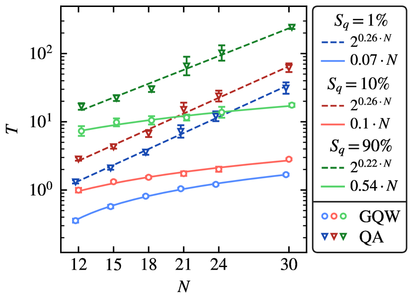
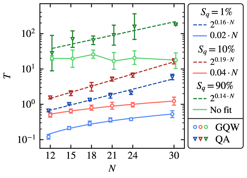
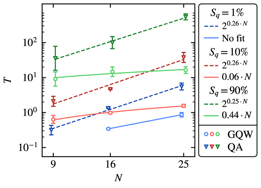
The previous section has demonstrated the efficiency of the proposed guiding procedure for quantum walks in solving combinatorial optimization problems. The GQW outperforms both the QW and QA by producing significantly higher solution qualities across all studied problem instances and evolution times $T$. However, to determine how these algorithms compare for real-world problem sizes ($N\gg 1$) that exceed the capabilities of our numerical simulations, we analyze the scaling of the evolution time $T_{S_{q}}(N)$ required to reach a solution quality $S_{q}\in\left\{1\%,10\%,90\%\right\}$ as a function of the problem size $N$. The corresponding data is shown in Fig. 8a together with linear ($a+b\cdot N$) and exponential ($a\cdot 2^{b\cdot N}$) fits to the data points obtained by the GQW and QA, respectively. The QW was excluded from this analysis, as it could not reach the required solution qualities. It’s worth noting that the QW is not designed as a single-shot algorithm, and we will discuss the multi-shot QW in the subsequent section.

The data shows, that QA exhibits exponential scaling, with similar scaling coefficients $b$ for the three solution quality levels $S_{q}$. This is in line with the expectation derived from the adiabatic theorem, as the instantaneous energy gaps, which shrink exponentially in $N$, demand an exponentially slow annealing process for the system to remain in its instantaneous ground state. In contrast, $T_{S_{q}}(N)$ follows a linear scaling in $N$ for the GQW. This can be explained by the fact that the depth of a hypercube graph scales linearly in the number of qubits $N$ (i.e., the largest Hamming distance between any two states cannot be larger than $N$). Hence, the GQW must at most drive amplitude transfers within $N$ local subspaces to transport amplitude from any state into the solution state. Since the Hamming distance from $z_{opt}$ to each computational basis state seems to correlate positively with the energy gaps of these states (cf. Fig. 3b), these amplitude transfers are performed simultaneously for all states, yielding a linear in $N$ evolution time $T$. In the regime of large $T$, the GQW can thus be seen as an optimized annealing schedule, where the algorithm selectively spends more time in critical parts of the graph (near the smallest instantaneous energy gap), while progressing faster elsewhere.

Although more extensive studies are required to verify the observation of a linear scaling, our findings frame the GQW as a highly efficient algorithm, allowing to obtain high solution qualities within short time scales. This makes the GQW an attractive choice for near-term quantum devices with limited coherence times.

IV.3 Classical optimization phase

We have examined the performance of the GQW, showcasing its capability to achieve optimal quantum evolutions by guiding amplitude transfers locally in the hypercube graph. Our findings indicate a linear scaling of the total evolution time $T_{S_{q}}(N)$ with respect to the problem size $N$, surpassing the performance of both the QW and the QA when provided with an optimal set of hyperparameters $\boldsymbol{\lambda}$. However, our investigation has primarily focused on the quantum aspect of this hybrid algorithm, without counting the classical optimization phase responsible for fine-tuning the six hyperparameters $\boldsymbol{\lambda}$.

Figure 8: Scaling of the total evolution time $T_{S_{q}}(N)$ required to achieve a specified solution quality $S_{q}$ on EC problems as a function of the problem size $N$ for the GQW (circles) and linear QA (triangles). Colors indicate results for various target solution qualities: $S_{q}=1\%$ (blue), $S_{q}=10\%$ (red), and $S_{q}=90\%$ (green). The solid lines depict linear fits ($a+b\cdot N$), while the dashed lines represent exponential fits ($a\cdot 2^{b\cdot N}$) applied to the data points (see legend).

Figure 9: Scaling analysis of the solution quality $S_{q}$ as a function of the total evolution time $T$ and the number of parameter evaluations $N_{opt}$ performed by the Nelder-Mead algorithm during the classical optimization phase of the hyperparameters $\boldsymbol{\lambda}$ in the GQW. Panels (a)–(e) depict the results for EC problems of sizes $N\in\left\{12,15,18,21,24\right\}$, respectively. The data is sampled with a granularity of $\Delta T=1$ and $\Delta N_{opt}=5$. Each data point represents the average solution quality obtained from $100$ repetitions of the optimization phase. Furthermore, the data is averaged across $10$ random problem instances for each problem size $N$. The blue circles mark the configurations of $T$ and $N_{opt}$ that yield the lowest $TTS_{99.99\%}$ (see Eq. (19)). The dashed curves indicate exponential fits to the $S_{q}=0.5$ contour. In panel (f) we show the scaling of the optimal (smallest) $TTS_{99.99\%}$ achieved by the GQW (blue), linear QA (red), and the QW (green) as a function of the problem size $N$. The solid lines correspond to exponential fits ($a\cdot 2^{b\cdot N}$) applied to the data points.

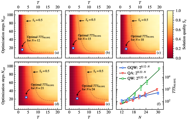
In Fig. 9, we investigate the influence of the classical optimization phase on the GQW by analyzing the scaling of the average solution quality $S_{q}$ as a function of the total evolution time $T$ and the number of parameter evaluations $N_{opt}$. The latter refers to the number of iterations performed by the Nelder-Mead algorithm during the initial optimization phase. Panels (a)–(e) present the averaged results for the EC problems with sizes $N\in\left\{12,15,18,21,24\right\}$, respectively.

The data reveals consistent characteristics across all investigated problem instances. Specifically, we observe that the number of parameter evaluations $N_{opt}^{S_{q}}$ necessary to reach a minimum solution quality $S_{q}$ decreases exponentially as a function of the total evolution time $T$ (see dashed curves in panels (a)–(e)). Additionally, for a fixed value of $T$, $N_{opt}^{S_{q}}$ scales exponentially in the problem size $N$. These observations indicate that for short evolutions, where the GQW prepares QW-like hopping rate schedules, the parameter search space tends to be more complex, thereby requiring longer optimization phases. This complexity arises, as the GQW is considering only a few subspaces, making it crucial to precisely set the hyperparameters $\boldsymbol{\lambda}$ to effectively drive amplitude transfers within these subspaces. Notably, the performance of the GQW is particularly sensitive to the choice of $\lambda_{5}$ and $\lambda_{6}$ in this regime of $T$. On the other hand, in the case of long evolutions, high-quality solutions can be obtained with just a few iterations from the classical optimizer. This is because deviations from the optimal schedule $\Gamma(t)$ have minimal impact on the overall evolution of the quantum system, as the optimal hopping rate schedules approach a QA-like evolution, and success is increasingly guaranteed by the adiabatic theorem.

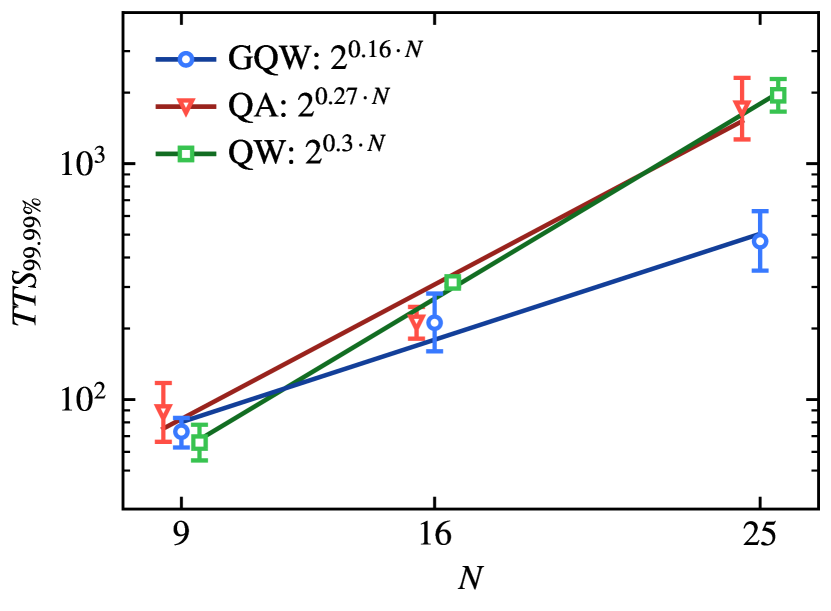
To incorporate the classical optimization phase into our performance evaluations, we consider the time-to-solution

$$TTS_{P_{target}}=\frac{\ln\left(1-P_{target}\right)}{\ln\left(1-P_{gs}\right)}\cdot T+N_{opt}\cdot T,$$ (19)

where $P_{gs}$ and $T$ denote the success probability and the evolution time of the algorithm, respectively. $TTS_{P_{target}}$ represents the total run time required to measure the solution state $\ket{z_{opt}}$ at least once, with a probability of $P_{target}$, over multiple runs of the algorithm. Note that the optimization phase is accounted for through the offset $N_{opt}\cdot T$.

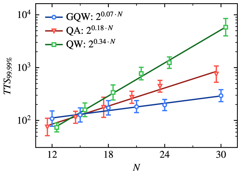
In Fig. 9f, we show a comparison of the scaling of the optimal (smallest) $TTS_{99.99\%}$ achieved by the GQW, the QW, and linear QA as a function of the problem size $N$. Exponential fits ($a\cdot 2^{b\cdot N}$) are included as a reference. The data reveals that for small problem sizes, both the QW and linear QA demonstrate faster convergence to the solution state compared to the GQW, due to the GQW’s initial optimization phase. However, for $N\geq 15$ and $N\geq 21$, respectively, the GQW surpasses both algorithms with a scaling factor of $b=0.12$, which is approximately four (two) times better than $b=0.47$ ($b=0.22$) for the QW (QA). Although the initial optimization phase in the GQW leads to an exponential scaling of $TTS_{99.99\%}$, the GQW’s ability to focus solely on a subset of the graph for small values of $T$ (intermediate evolutions) enables a significantly more efficient utilization of computational resources compared to the other algorithms. Furthermore, the fact that the exponential scaling is shifted into the optimization phase, while the single run times $T$ scale at most linearly with $N$ (see Sec. IV.2), offers the opportunity to distribute the optimization phase across multiple quantum computing devices, thereby providing an option to parallelize the process. This is a feature generally not feasible for QA due to the exponential scaling of $T$, but it could potentially allow solving large optimization problems on near-term quantum devices.

V Conclusion

We have utilized the theory of local amplitude transfers (LAT), which offers a new perspective on the operational principles of quantum annealing (QA) and quantum walks (QWs) beyond the adiabatic theorem, while also providing insights into the design of optimal quantum evolutions. The theory is rooted in the description of a quantum evolution within the eigenspace of the problem Hamiltonian $\hat{H}_{C}$. In this context, the search space is represented as a graph $G$ where the states are interconnected through the driving Hamiltonian $\hat{H}_{D}$ (see Fig. 3a). By decomposing $G$ into two-dimensional subspaces spanned by pairs of eigenstates, we have demonstrated that probability amplitude traverses the graph through a sequence of local Rabi oscillations occurring within these subspaces. The amplitude of these oscillations depends on the relative strengths of the local driving and problem Hamiltonians, controlled by the hopping rate $\Gamma$.

We have highlighted that for sufficiently complex problems, the average energy gap of the local problem Hamiltonian monotonically increases as a function of the energy level (see Fig. 3b), allowing to selectively drive amplitude transfers within distinct regions of the graph. This property provides a new understanding of how probability amplitude propagates through the search space during continuous-time quantum algorithms.

In particular, we have identified QWs and QA as two formulations of the same underlying principle (see Fig. 6), with QA corresponding to a sequence of distinct QWs with gradually decreasing hopping rates $\Gamma$. We have shown that a QW-like approach employing a small and constant hopping rate is generally optimal for short evolutions, as it allows for localized dynamics near the solution state. However, it becomes suboptimal for long evolutions, as it fails to effectively transfer amplitude from higher energy states. Conversely, a QA-like strategy is preferred for long evolutions, as it guides amplitude throughout the entire graph, but it is suboptimal for short evolutions, since it spends insufficient time in subspaces near the solution state. Based on these insights, we have argued that optimal quantum evolutions must adapt to the total evolution time $T$ by striking a balance between the number of guided local subspaces (representing the amount of guided amplitude) and the time spent at each energy level (reflecting the amount of amplitude transferred within each local subspace).

Within the LAT framework, we have introduced the guided quantum walk (GQW) as a promising approach for solving large-scale combinatorial optimization problems in the transition region between QWs and QA. The GQW progressively drives local subspaces at gradually decreasing energy levels by utilizing a monotonically decreasing hopping rate $\Gamma(t)$. The hopping rate is controlled through a cubic Bézier curve (see Fig. 5) defined by six hyperparameters, which allows for fine-tuning the quantum evolution to each problem instance (i.e., energy spectrum of $\hat{H}_{C}$) and evolution time $T$.

We assessed the performance of the GQW in comparison to QA and optimized QWs on exact cover (EC), traveling salesperson (TSP), and garden optimization (GO) problems ranging from $9$ to $30$ qubits. Across all investigated problem instances and evolution times $T$, the GQW outperformed both the QW and QA significantly. Specifically, at intermediate timescales, our data reveals an up to four (three) orders of magnitude better performance on $30$ qubit problems compared to QA (QW), see Fig. 7. This observation is further supported by the scaling of the minimal evolution time necessary to reach a fixed solution quality as a function of the problem size. In contrast to the exponential scaling observed for QA, the GQW demonstrates a linear scaling, strongly indicating the existence of optimal quantum evolutions that solve combinatorial optimization problems in linear time $T$, thus surpassing the limitations of adiabatic time evolutions.

It is worth noting that the achieved linear scaling is made possible by shifting the exponential scaling to the classical optimization phase of the hyperparameters. Nonetheless, even when considering the parameter tuning in the total run time, the GQW exhibits a time-to-solution scaling that is approximately two (four) times better than for QA (QWs), see Fig. 9f. This positions the GQW as a powerful tool for deriving optimal annealing schedules. Furthermore, the presence of the exponential scaling in the classical optimization phase, rather than in the single run times, offers the opportunity to distribute the optimization phase across multiple quantum computing devices, thereby enabling parallelization of the process. Moreover, short evolution times also suggest the possibility of discretizing the GQW into a few time steps, therefore adapting the Bézier curve parametrization into a QAOA-like scheme on gate-based quantum computers. These are features generally not feasible for QA due to the exponential scaling of $T$, but it could potentially allow solving large optimization problems on near-term quantum devices. While further investigation is needed to determine how these observations translate to real quantum devices in the presence of environmental noise and on problems with non-canonical energy spectra (e.g., with large degeneracies), our results strongly support the practicality of the GQW for real-world optimization problems, and we expect that our strategy is easily applicable to other types of optimization problems, beyond EC, TSP and GO instances.

Appendix A Problem cost functions

In this appendix, we provide an overview of the cost functions $C(z)$ for the EC, TSP, and GO problems under investigation.

A.1 Exact cover problem

The EC problem [33, 2] involves a set $U=\left\{x_{0},x_{1},\dots,x_{P-1}\right\}$ with $P$ distinct elements and $N$ subsets $V_{i}\subseteq U$, such that $U=\bigcup_{i}V_{i}$. An EC is a subset $L$ of the set of sets $\left\{V_{i}\right\}$, such that the elements of $L$ are disjoint sets, and their union is $U$. The problem can be expressed in matrix form using a Boolean problem matrix $A\in\left\{0,1\right\}^{N\times P}$, where the matrix columns refer to the $P$ elements $x_{k}$ in $U$ and the matrix rows correspond to the $N$ subsets $V_{i}$. If $A_{ik}=1$, then element $x_{k}$ is included in subset $V_{i}$, otherwise not. Thus, $L$ is the subset of matrix rows such that the entry $1$ appears in each column exactly once, leading to the cost function

$$C\left(z\right) =\sum_{k=0}^{P-1}\left[\sum_{i=0}^{N-1}A_{ik}z_{i}-1\right]^{2},$$ (20)

where $z\in\left\{0,1\right\}^{\otimes N}$ encodes the selection of subsets $V_{i}$. Note that the minimum of $C\left(z\right)$ is zero and represents the EC solution. By expanding the square and collecting linear, quadratic, and constant terms in $z_{i}$, we obtain the QUBO coefficients

$$Q_{ij}=P+\begin{cases}\sum_{k=0}^{P}2A_{ik}A_{jk},\quad&i<j\\ \sum_{k=0}^{P}A_{ik}\cdot\left(A_{ik}-2\right),\quad&i=j\end{cases}.$$ (21)

A.2 Traveling salesperson problem

The TSP problem [35, 36, 37, 7, 38] involves a list of $M$ locations and a cost matrix $c_{kj}$ between each pair of locations $\left(k,j\right)$. The goal is to find the most optimal route, with the lowest total cost, that visits each location exactly once and returns to its starting location. We represent the problem using a Boolean problem matrix $A\in\left\{0,1\right\}^{M\times M}$, where the matrix rows correspond to the $M$ locations, and the matrix columns denote the order in which the locations are visited. If $A_{k,j}=1$, then the location $k$ is visited at time step $j$, otherwise not. The solution to the TSP problem is the lowest-cost arrangement of $0$’s and $1$’s in $A$, such that an $1$ is contained in each row and in each column exactly once, leading to the cost function

$$C\left(z\right)= \lambda\sum_{k=0}^{M-1}\sum_{j=0}^{M-1}\sum_{t=0}^{M-1}c_{kj}z_{kM+t}z_{jM+t+1}$$

$$+\sum_{k=0}^{M-1}\left[\sum_{t=0}^{M-1}z_{kM+t}-1\right]^{2}$$

$$+\sum_{t=0}^{M-1}\left[\sum_{k=0}^{M-1}z_{kM+t}-1\right]^{2},$$ (22)

with $z_{i}=A_{k,j}$ with $i=kM+j$ and $\lambda$ denoting a free parameter to scale the cost matrix with respect to the constraints. We can determine the QUBO coefficients $Q_{ii^{\prime}}$ by stepping through the terms in Eq. (22) and summing up the respective contributions. It is important to note that we fix the starting location, reducing the number of problem variables $z_{i}$ to $\left(M-1\right)^{2}$. Moreover, the number of optimal routes is even because each route can be travelled in one direction or the other.

A.3 Garden optimization problem

The GO problem was first introduced by Gonzalez Calaza et al. [39] and refers to the problem of arranging plants in a garden. The garden is represented by $M$ pots randomly distributed on a grid, with a Boolean matrix $J\in\left\{0,1\right\}^{M\times M}$ encoding the adjacency of pots. Given $P$ distinct plant species, with $c_{j}$ plants per species, the goal of the GO problem is to find the optimal arrangement of plants in the pots with respect to the relationships between different plant species. These relationships are encoded in the companions matrix $A\in\left\{-1,0,1\right\}^{P\times P}$, yielding the cost function

$$C\left(z\right)= \sum_{k,k^{\prime}=0}^{M-1}J_{k,k^{\prime}}\left[1+\sum_{j,j^{\prime}=0}^{P-1}z_{kP+j}A_{j,j^{\prime}}z_{k^{\prime}P+j^{\prime}}\right]$$

$$+\lambda_{1}\sum_{k=0}^{M-1}\left[1-\sum_{j=0}^{P-1}z_{kP+j}\right]^{2}$$

$$+\lambda_{2}\sum_{j=0}^{P-1}\left[c_{j}-\sum_{k=0}^{M-1}z_{kP+j}\right]^{2},$$ (23)

where $\lambda_{1}$ and $\lambda_{2}$ are free parameters. The $M\times P$ Boolean problem variables $z$ indicate whether a plant of species $j$ is placed in pot $k$ (i.e., $z_{kP+j}=1$) or not. By stepping through the terms in Eq. (23) and summing up the respective contributions, we can determine the QUBO coefficients $Q_{ii^{\prime}}$ in the same way as for the other problems.

Appendix B GO and TSP results

In this appendix, we present the simulation results for the GQW, the QW, and QA applied to GO and TSP problems. We investigate GO problems with problem sizes $N\in\left\{12,15,18,21,24,30\right\}$ and TSP problems with problem sizes $N\in\left\{9,16,25\right\}$, considering a total of $10$ randomly generated instances for each problem size and type. Similar to the EC results from the main text, the GQW and the QW are tuned for each problem instance and evolution time $T$ separately by optimizing their hyperparameters to minimize the energy expectation value $E_{\Psi}$ of the final quantum state $\ket{\Psi}$. Each set of hyperparameters is selected from a pool of $N_{rep}=100$ runs of the Nelder-Mead classical optimizer, where for each run, the hyperparameters are initialized randomly and adjusted up to a maximum of $N_{eval}=100$ times. The QA results are obtained using a linear annealing scheme.

Figures 10 and 13 depict the scaling of the solution quality $S_{q}$ as a function of the evolution time $T$ and the problem size $N$ for the three algorithms on GO and TSP problems, respectively. The data exhibit similar characteristics to the EC problems presented in Fig. 7 and are qualitatively consistent with the discussion in Sec. IV.1. Notably, the GQW achieves higher solution qualities for some large GO problems (e.g., $N=30$) compared to some smaller problem sizes (e.g., $N=18$) for long evolutions (see inset in Fig. 10a). This indicates that the hardness of the combinatorial optimization problems varies throughout the problem sizes, such that some large problem instances are easier to solve than their small counterparts once the GQW considers the entire graph. Consequently, we expect similar characteristics in the scaling of $S_{q}$ to appear for QA for long evolutions.

In Figures 12 and 15, we present the scaling of the minimum evolution time $T_{S_{q}}(N)$ required to achieve a specified solution quality $S_{q}$ as a function of the problem size $N$. Similar to the results obtained for the EC problems, $T_{S_{q}}(N)$ exhibits linear scaling for the GQW, in contrast to the exponential scaling observed for QA. This further supports the existence of optimal hopping rate schedules that can solve combinatorial optimization problems in linear time. Note, however, that for the GO problems, $T_{0.9}(N)$ neither corresponds to an exponential nor a linear scaling, due to the differences in the hardness of the optimization problems.

Figures 12 and 15 show the scaling of the time-to-solution (see Eq. (19)) as a function of the problem size $N$. For both problem types, the GQW achieves a superior scaling compared to QA and the QW by factors of $\approx 2$ (QA on GO problems), $\approx 4$ (QW on GO problems) and $\approx 2$ (QA and QW on TSP problems).

Figure 10: Performance comparison of (a) the GQW, (b) the QW, and (c) QA as a function of the total evolution time $T$ on GO problems with problem sizes $N\in\left\{12,15,18,21,24,30\right\}$ (see legend). The performance is assessed based on the solution quality $S_{q}$ defined in (4). Each problem size $N$ is evaluated using a set of $10$ randomly generated instances, and the presented data corresponds to the geometric mean solution qualities (solid curves) along with the geometric standard deviations (shaded areas). Note that the GQW and the QW undergo a prior classical optimization phase. The dotted gray lines indicate horizontal cuts ($S_{q}\in\left\{1\%,10\%,90\%\right\}$), which are detailed in Fig. 12. The inset in panel (a) provides a zoomed-in view of the region corresponding to large evolution times $T$. Additionally, the dashed lines in panel (b) indicate the stationary solution quality that the damped oscillation of $S_{q}(T)$ approaches for the QW at large $T$.

Figure 11: Scaling behavior of the total evolution time $T_{S_{q}}(N)$ required to achieve a specified solution quality $S_{q}$ on GO problems as a function of the problem size $N$ for the GQW (circles) and linear QA (triangles). Colors indicate results for various target solution qualities: $S_{q}=1\%$ (blue), $S_{q}=10\%$ (red), and $S_{q}=90\%$ (green). The solid lines depict linear fits ($a+b\cdot N$), while the dashed lines represent exponential fits ($a\cdot 2^{b\cdot N}$) applied to the data points (see legend).

Figure 12: Scaling analysis of the optimal (smallest) time-to-solution $TTS_{99.99\%}$ (see Eq. (19)) for the GQW (blue), QA (red), and the QW (green) on GO problems as a function of the problem size $N$. The solid lines correspond to exponential fits ($a\cdot 2^{b\cdot N}$) applied to the data points (see legend).

Figure 13: Performance comparison of (a) the GQW, (b) the QW, and (c) QA as a function of the total evolution time $T$ on TSP problems with problem sizes $N\in\left\{9,16,25\right\}$ (see legend). The performance is assessed based on the solution quality $S_{q}$ defined in (4). Each problem size $N$ is evaluated using a set of $10$ randomly generated instances, and the presented data corresponds to the geometric mean solution qualities (solid curves) along with the geometric standard deviations (shaded areas). Note that the GQW and the QW undergo a prior classical optimization phase. The dotted gray lines indicate horizontal cuts ($S_{q}\in\left\{1\%,10\%,90\%\right\}$), which are detailed in Fig. 15. The inset in panel (a) provides a zoomed-in view of the region corresponding to large evolution times $T$. Additionally, the dashed lines in panel (b) indicate the stationary solution quality that the damped oscillation of $S_{q}(T)$ approaches for the QW at large $T$.

Figure 14: Scaling behavior of the total evolution time $T_{S_{q}}(N)$ required to achieve a specified solution quality $S_{q}$ on TSP problems as a function of the problem size $N$ for the GQW (circles) and linear QA (triangles). Colors indicate results for various target solution qualities: $S_{q}=1\%$ (blue), $S_{q}=10\%$ (red), and $S_{q}=90\%$ (green). The solid lines depict linear fits ($a+b\cdot N$), while the dashed lines represent exponential fits ($a\cdot 2^{b\cdot N}$) applied to the data points (see legend).

Figure 15: Scaling analysis of the optimal (smallest) time-to-solution $TTS_{99.99\%}$ (see Eq. (19)) for the GQW (blue), QA (red), and the QW (green) on TSP problems as a function of the problem size $N$. The solid lines correspond to exponential fits ($a\cdot 2^{b\cdot N}$) applied to the data points (see legend).

References

- Marzec [2016] M. Marzec, Portfolio Optimization: Applications in Quantum Computing, Handbook of High‐Frequency Trading and Modeling in Finance , 73 (2016).
- Willsch et al. [2022] D. Willsch, M. Willsch, C. D. G. Calaza, F. Jin, H. De Raedt, M. Svensson, and K. Michielsen, Benchmarking Advantage and D-Wave 2000Q quantum annealers with exact cover problems, Quantum Information Processing 21, 10.1007/s11128-022-03476-y (2022).
- Amin et al. [2018] M. H. Amin, E. Andriyash, J. Rolfe, B. Kulchytskyy, and R. Melko, Quantum Boltzmann Machine, Physical Review X 8, 10.1103/physrevx.8.021050 (2018).
- Benedetti et al. [2016] M. Benedetti, J. Realpe-Gómez, R. Biswas, and A. Perdomo-Ortiz, Estimation of effective temperatures in quantum annealers for sampling applications: A case study with possible applications in deep learning, Phys. Rev. A 94, 022308 (2016).
- Childs and Goldstone [2004] A. M. Childs and J. Goldstone, Spatial search by quantum walk, Phys. Rev. A 70, 022314 (2004).
- Perdomo-Ortiz et al. [2012] A. Perdomo-Ortiz, N. Dickson, M. Drew-Brook, G. Rose, and A. Aspuru-Guzik, Finding low-energy conformations of lattice protein models by quantum annealing, Scientific Reports 10.1038/srep00571 (2012).
- Boucherie et al. [2021] R. J. Boucherie, A. Braaksma, and H. Tijms, Operations Research (World Scientific, 2021).
- Preskill [2018] J. Preskill, Quantum Computing in the NISQ era and beyond, Quantum 2, 79 (2018).
- Aharonov et al. [1993] Y. Aharonov, L. Davidovich, and N. Zagury, Quantum random walks, Phys. Rev. A 48, 1687 (1993).
- Childs et al. [2002] A. M. Childs, E. Deotto, E. Farhi, J. Goldstone, S. Gutmann, and A. J. Landahl, Quantum search by measurement, Phys. Rev. A 66, 032314 (2002).
- Callison et al. [2021] A. Callison, M. Festenstein, J. Chen, L. Nita, V. Kendon, and N. Chancellor, Energetic Perspective on Rapid Quenches in Quantum Annealing, PRX Quantum 2, 010338 (2021).
- Banks et al. [2023] R. J. Banks, E. Haque, F. Nazef, F. Fethallah, F. Ruqaya, H. Ahsan, H. Vora, H. Tahir, I. Ahmad, I. Hewins, I. Shah, K. Baranwal, M. Arora, M. Asad, M. Khan, N. Hasan, N. Azad, S. Fedaiee, S. Majeed, S. Bhuyan, T. Tarannum, Y. Ali, D. E. Browne, and P. A. Warburton, Continuous-time quantum walks for MAX-CUT are hot, arXiv:2306.10365 [quant-ph] (2023).
- Apolloni et al. [1989] B. Apolloni, C. Carvalho, and D. de Falco, Quantum stochastic optimization, Stoch. Process. Their Appl. 33, 233 (1989).
- Finnila et al. [1994] A. Finnila, M. Gomez, C. Sebenik, C. Stenson, and J. Doll, Quantum annealing: A new method for minimizing multidimensional functions, Chem. Phys. Lett. 219, 343 (1994).
- Kadowaki and Nishimori [1998] T. Kadowaki and H. Nishimori, Quantum annealing in the transverse Ising model, Phys. Rev. E 58, 5355 (1998).
- Brooke et al. [1999] J. Brooke, D. Bitko, T. F. Rosenbaum, and G. Aeppli, Quantum Annealing of a Disordered Magnet, Science 284, 779 (1999).
- Johnson et al. [2011] M. W. Johnson, M. H. S. Amin, S. Gildert, T. Lanting, F. Hamze, N. Dickson, R. Harris, A. J. Berkley, J. Johansson, P. Bunyk, E. M. Chapple, C. Enderud, J. P. Hilton, K. Karimi, E. Ladizinsky, N. Ladizinsky, T. Oh, I. Perminov, C. Rich, M. C. Thom, E. Tolkacheva, C. J. S. Truncik, S. Uchaikin, J. Wang, B. Wilson, and G. Rose, Quantum annealing with manufactured spins, Nature 473, 194 (2011).
- Harris et al. [2010] R. Harris, M. W. Johnson, T. Lanting, A. J. Berkley, J. Johansson, P. Bunyk, E. Tolkacheva, E. Ladizinsky, N. Ladizinsky, T. Oh, F. Cioata, I. Perminov, P. Spear, C. Enderud, C. Rich, S. Uchaikin, M. C. Thom, E. M. Chapple, J. Wang, B. Wilson, M. H. S. Amin, N. Dickson, K. Karimi, B. Macready, C. J. S. Truncik, and G. Rose, Experimental investigation of an eight-qubit unit cell in a superconducting optimization processor, Phys. Rev. B 82, 024511 (2010).
- Bunyk et al. [2014] P. I. Bunyk, E. M. Hoskinson, M. W. Johnson, E. Tolkacheva, F. Altomare, A. J. Berkley, R. Harris, J. P. Hilton, T. Lanting, A. J. Przybysz, and J. Whittaker, Architectural Considerations in the Design of a Superconducting Quantum Annealing Processor, IEEE Transactions on Applied Superconductivity 24, 1 (2014).
- Albash and Lidar [2018a] T. Albash and D. A. Lidar, Adiabatic quantum computation, Rev. Mod. Phys. 90, 015002 (2018a).
- Albash and Lidar [2018b] T. Albash and D. A. Lidar, Demonstration of a Scaling Advantage for a Quantum Annealer over Simulated Annealing, Phys. Rev. X 8, 031016 (2018b).
- King et al. [2023] A. D. King, J. Raymond, T. Lanting, R. Harris, A. Zucca, F. Altomare, A. J. Berkley, K. Boothby, S. Ejtemaee, C. Enderud, E. Hoskinson, S. Huang, E. Ladizinsky, A. J. R. MacDonald, G. Marsden, R. Molavi, T. Oh, G. Poulin-Lamarre, M. Reis, C. Rich, Y. Sato, N. Tsai, M. Volkmann, J. D. Whittaker, J. Yao, A. W. Sandvik, and M. H. Amin, Quantum critical dynamics in a 5,000-qubit programmable spin glass, Nature 617, 61 (2023).
- Callison et al. [2019] A. Callison, N. Chancellor, F. Mintert, and V. Kendon, Finding spin glass ground states using quantum walks, New Journal of Physics 21, 123022 (2019).
- Neuhaus [2014a] T. Neuhaus, Monte Carlo Search for Very Hard KSAT Realizations for Use in Quantum Annealing, arXiv:1412.5361 [cond-mat.stat-mech] (2014a).
- Neuhaus [2014b] T. Neuhaus, Quantum Searches in a Hard 2SAT Ensemble, arXiv:1412.5460 [quant-ph] (2014b).
- Mehta et al. [2021] V. Mehta, F. Jin, H. De Raedt, and K. Michielsen, Quantum annealing with trigger Hamiltonians: Application to 2-satisfiability and nonstoquastic problems, Phys. Rev. A 104, 032421 (2021).
- Mehta et al. [2022a] V. Mehta, F. Jin, H. De Raedt, and K. Michielsen, Quantum annealing for hard 2-satisfiability problems: Distribution and scaling of minimum energy gap and success probability, Phys. Rev. A 105, 062406 (2022a).
- Mehta et al. [2022b] V. Mehta, F. Jin, K. Michielsen, and H. De Raedt, On the hardness of quadratic unconstrained binary optimization problems, Front. Phys. 10, 956882 (2022b).
- Morley et al. [2019] J. G. Morley, N. Chancellor, S. Bose, and V. Kendon, Quantum search with hybrid adiabatic–quantum-walk algorithms and realistic noise, Phys. Rev. A 99, 022339 (2019).
- Lishan Zeng, Jun Zhang and Mohan Sarovar [2016] Lishan Zeng, Jun Zhang and Mohan Sarovar, Schedule path optimization for adiabatic quantum computing and optimization, Journal of Physics A: Mathematical and Theoretical 10.1088/1751-8113/49/16/165305 (2016).
- Herr et al. [2017] D. Herr, E. Brown, B. Heim, M. Könz, G. Mazzola, and M. Troyer, Optimizing Schedules for Quantum Annealing, arXiv:1705.00420 (2017).
- Yu-Qin Chen and Yu Chen and Chee-Kong Lee and Shengyu Zhang and Chang-Yu Hsieh [2022] Yu-Qin Chen and Yu Chen and Chee-Kong Lee and Shengyu Zhang and Chang-Yu Hsieh, Optimizing Quantum Annealing Schedules with Monte Carlo Tree Search enhanced with neural networks, Nature Machine Intelligence 10.1038/s42256-022-00446-y (2022).
- Karp [1972] R. M. Karp, Reducibility among Combinatorial Problems, in Complexity of Computer Computations: Proceedings of a symposium on the Complexity of Computer Computations, held March 20–22, 1972, at the IBM Thomas J. Watson Research Center, Yorktown Heights, New York, and sponsored by the Office of Naval Research, Mathematics Program, IBM World Trade Corporation, and the IBM Research Mathematical Sciences Department, edited by R. E. Miller, J. W. Thatcher, and J. D. Bohlinger (Springer US, Boston, MA, 1972) pp. 85–103.
- Choi [2010] V. Choi, Adiabatic Quantum Algorithms for the NP-Complete Maximum-Weight Independent Set, Exact Cover and 3SAT Problems, (2010), arXiv:1004.2226 [quant-ph] .
- Dantzig et al. [1954] G. Dantzig, R. Fulkerson, and S. Johnson, Solution of a Large-Scale Traveling-Salesman Problem, J. Oper. Res. Soc. Am. 2, 393 (1954).
- Bellman [1962] R. Bellman, Dynamic Programming Treatment of the Travelling Salesman Problem, J. ACM 9, 61 (1962).
- Held and Karp [1962] M. Held and R. M. Karp, A Dynamic Programming Approach to Sequencing Problems, Journal of the Society for Industrial and Applied Mathematics 10, 196 (1962).
- Lucas [2014] A. Lucas, Ising formulations of many NP problems, Front. Phys. 2, 5 (2014).
- Gonzalez Calaza et al. [2021] C. D. Gonzalez Calaza, D. Willsch, and K. Michielsen, Garden optimization problems for benchmarking quantum annealers, Quantum Inf. Process. 20, 305 (2021).
- Jülich Supercomputing Centre [2021] Jülich Supercomputing Centre, JUWELS Cluster and Booster: Exascale Pathfinder with Modular Supercomputing Architecture at Juelich Supercomputing Centre, J. of Large-Scale Res. Facil. 7, A138 (2021).
- Grover [1996] L. K. Grover, A Fast Quantum Mechanical Algorithm for Database Search, in Proceedings of the Twenty-Eighth Annual ACM Symposium on Theory of Computing, STOC ’96 (Association for Computing Machinery, New York, NY, USA, 1996) p. 212–219.
- Farhi et al. [2014] E. Farhi, J. Goldstone, and S. Gutmann, A Quantum Approximate Optimization Algorithm, arXiv:1411.4028 [quant-ph] (2014).
- McClean et al. [2016] J. R. McClean, J. Romero, R. Babbush, and A. Aspuru-Guzik, The theory of variational hybrid quantum-classical algorithms, New J. Phys. 18, 023023 (2016).
- Tilly et al. [2022] J. Tilly, H. Chen, S. Cao, D. Picozzi, K. Setia, Y. Li, E. Grant, L. Wossnig, I. Rungger, G. H. Booth, and J. Tennyson, The Variational Quantum Eigensolver: A review of methods and best practices, Phys. Rep. 986, 1 (2022).
- Farhi et al. [2000] E. Farhi, J. Goldstone, S. Gutmann, and M. Sipser, Quantum Computation by Adiabatic Evolution, arXiv:quant-ph/0001106 (2000).
- Zhou et al. [2020] L. Zhou, S.-T. Wang, S. Choi, H. Pichler, and M. D. Lukin, Quantum Approximate Optimization Algorithm: Performance, Mechanism, and Implementation on Near-Term Devices, Phys. Rev. X 10, 021067 (2020).
- Sack and Serbyn [2021] S. H. Sack and M. Serbyn, Quantum annealing initialization of the quantum approximate optimization algorithm, Quantum 5, 491 (2021).
- Nelder and Mead [1965] J. A. Nelder and R. Mead, A Simplex Method for Function Minimization, Comput. J. 7, 308 (1965).
- Press et al. [2007] W. H. Press, S. A. Teukolsky, W. T. Vetterling, and B. P. Flannery, Numerical Recipes 3rd Edition: The Art of Scientific Computing (Cambridge University Press, New York, USA, 2007).
- Suzuki [1993] M. Suzuki, General Decomposition Theory of Ordered Exponentials, Proc. Japan Acad. B 69, 161 (1993).
- De Raedt and Michielsen [2006] H. De Raedt and K. Michielsen, Computational Methods for Simulating Quantum Computers, in Quantum and Molecular Computing, Quantum Simulations, Handbook of Theoretical and Computational Nanotechnology, Vol. 3, edited by M. Rieth and W. Schommers (American Scientific, Los Angeles, 2006) pp. 1–48.
- Crosson et al. [2014] E. Crosson, E. Farhi, C. Y.-Y. Lin, H.-H. Lin, and P. Shor, Different Strategies for Optimization Using the Quantum Adiabatic Algorithm, (2014), arXiv:1401.7320 [quant-ph] .
- Crosson and Lidar [2021] E. J. Crosson and D. A. Lidar, Prospects for quantum enhancement with diabatic quantum annealing, Nature Reviews Physics 3, 466 (2021).