Unifying Distributionally Robust Optimization via Optimal Transport Theory

Abstract

In the past few years, there has been considerable interest in two prominent approaches for Distributionally Robust Optimization (DRO): Divergence-based and Wasserstein-based methods. The divergence approach models misspecification in terms of likelihood ratios, while the latter models it through a measure of distance or cost in actual outcomes. Building upon these advances, this paper introduces a novel approach that unifies these methods into a single framework based on optimal transport (OT) with conditional moment constraints. Our proposed approach, for example, makes it possible for optimal adversarial distributions to simultaneously perturb likelihood and outcomes, while producing an optimal (in an optimal transport sense) coupling between the baseline model and the adversarial model. Additionally, the paper investigates several duality results and presents tractable reformulations that enhance the practical applicability of this unified framework.

1 Introduction

DRO has gained popularity in uncertainty-based decision-making, mainly due to its ability to effectively address distribution ambiguity [Rahimian and Mehrotra,, 2022; Kuhn et al.,, 2019; Chen et al.,, 2020; Blanchet et al., 2021a, ; Lin et al.,, 2022].

There are two natural ways to model changes in distributions to build distributional ambiguity sets. The first way is to assume that the likelihood of the baseline model (often uniformly distributed over an observed data set) is corrupted. In this case, we may account for model misspecification using likelihood ratios. This leads to $\phi$-divergence-based uncertainty sets; see, e.g., [Hansen and Sargent,, 2001; Bertsimas and Sim,, 2004; El Ghaoui and Nilim,, 2005; Iyengar,, 2005; Lim et al.,, 2006; Bayraksan and Love, 2015a, ; Namkoong and Duchi,, 2016; Lam,, 2016; Wang et al.,, 2016; Breuer and Csiszár,, 2016; Namkoong and Duchi,, 2017; Hu and Hong,, 2013; Ben-Tal et al.,, 2009; Bertsimas et al.,, 2018; Jiang and Guan,, 2018; Lam,, 2019; Duchi and Namkoong,, 2021; Van Parys et al.,, 2021]. The second way is to account for potential corruptions in the baseline model by considering perturbations in the actual outcomes. This naturally leads to using the Wasserstein distance as an approach to quantify model misspecification in actual outcomes; see, e.g., [Scarf,, 1958; Pflug and Wozabal,, 2007; Sinha et al.,, 2018; Gao et al.,, 2022; Lee and Raginsky,, 2018; Pflug and Wozabal,, 2007; Mohajerin Esfahani and Kuhn,, 2018; Gao and Kleywegt, 2022a, ; Blanchet and Murthy,, 2019; Blanchet et al.,, 2019; Shafieezadeh-Abadeh et al.,, 2019; Xie,, 2021; Chen et al.,, 2022] and the references therein.

Traditionally, these two methods have been viewed as separate mechanisms that correspond to different types of phenomena. In this paper, we demonstrate that these methods can be unified under the framework of OT-DRO with suitable conditional moment constraints. As a result, this approach allows us to incorporate distributional uncertainty sets to model the model misspecification in terms of both likelihoods and actual outcomes under OT methods.

There are several advantages of the proposed unification approach under the umbrella of OT. First, a substantial amount of computational research has been conducted within both the OT-based DRO community [Sinha et al.,, 2018; Blanchet et al., 2021b, ; Li et al.,, 2019, 2020; Yu et al.,, 2022; Wang et al.,, 2021; Li,, 2021] and the OT community [Peyré et al.,, 2019; Gulrajani et al.,, 2017; Arjovsky et al.,, 2017; Cuturi,, 2013; Genevay et al.,, 2016; Seguy et al.,, 2018; Taşkesen et al.,, 2023] in recent years. Our approach has the potential to allow cross-dissemination and synergies between the methods developed in these communities. Second, the approach inherits the advantages of the OT framework, which, by construction, provides a coupling between the nominal and adversarial distributions. This feature improves interpretability and provides valuable modeling insights on the way in which each scenario would be modified to increase its impact on risk relative to a specific performance measure of interest. Lastly, the field of OT-DRO provides a substantial amount of theory that (we expect) can be easily adapted to our specific setting. This includes areas such as determining the optimal uncertainty size [Blanchet and Si,, 2019; Blanchet et al., 2021a, ; Blanchet et al.,, 2019, 2022], exploring the statistical properties of OT-DRO problems [He and Lam,, 2021; An and Gao,, 2021; Gao,, 2022; Aolaritei et al.,, 2022; Blanchet and Shapiro,, 2023; Azizian et al.,, 2023], interpreting least favorable distributions and Nash equilibrium [Mohajerin Esfahani and Kuhn,, 2018; Yue et al.,, 2021; Gao and Kleywegt, 2022b, ; Zhang et al., 2022b, ; Shafieezadeh-Abadeh et al.,, 2023], as well as establishing connections with different regularization approaches [Shafieezadeh Abadeh et al.,, 2015; Chen and Paschalidis,, 2018; Blanchet et al.,, 2019; Shafieezadeh-Abadeh et al.,, 2019; Cranko et al.,, 2021; Gao et al.,, 2022], just to name a few. Thus, we expect that this work will spark contributions in all of these areas from an encompassing perspective.

Structure of the paper

The paper is structured as follows. Section 2 provides an introduction to the problem setup and the key concepts used throughout the paper. In Section 3, we demonstrate how our proposed unification approach under OT can encompass various types of DRO problems. Section 4 presents a general strong duality theorem for the proposed OT-DRO model with conditional moment constraints. Upon this unification approach, we introduce a tractable transportation encompassing both $\phi$-divergence and Wasserstein ambiguity in Section 5. We visualize its worst-case distribution to gain insight into how to simultaneously perturb the actual outcome and the likelihood ratio in Section 6. Finally, we conclude with some final remarks in Section 7.

2 Problem Setup

Let us introduce the basic setup of the problem and key concepts that will serve as the basis for our subsequent analysis.

Notation. We denote by $[n]=\{1,\ldots,n\}$ the set of all integers up to $n\in\mathbb{N}$. Throughout the paper, we let $\mathbb{R}$ denote the set of real numbers, $\overline{\mathbb{R}}$ denote the set of extended real numbers, $\mathbb{R}_{+}$ denote the subset of non-negative real numbers. We adopt the conventions of extended arithmetics, whereby $\infty\cdot 0=0\cdot\infty=0/0=0$ and $\infty-\infty=-\infty+\infty=1/0=\infty$. We use capitalized letters for random variables, e.g., $Z,V,W$. We use mathcal for the sets, e.g., $\mathcal{Z},\mathcal{V},\mathcal{W}$. For a set $\mathcal{Z}\subset\mathbb{R}^{d}$, the indicator function $\mathbb{I}_{\mathcal{Z}}$ is defined by $\mathbb{I}_{\mathcal{Z}}(z)=1$ if $z\in\mathcal{Z}$; $=0$ otherwise. For any close set $\mathcal{Z}\subset\mathbb{R}^{d}$, we define $\mathcal{P}(\mathcal{Z})$ as the family of all Borel probability measures on $\mathcal{Z}$. For $\mu\in\mathcal{P}(\mathcal{Z})$, we use the notation $\mathbb{E}_{\mu}[\cdot]$ to denote expectation with respect to the probability distribution $\mu$. We define $\mathcal{L}_{1}(\mathrm{d}\mu)$ as the collection of Borel-measurable functions $f:\mathcal{Z}\rightarrow\mathbb{R}$ such that $\int_{\mathcal{Z}}|f(Z)|\mu(\mathrm{d}Z)<+\infty$. For an extended value function $f:\mathcal{Z}\rightarrow\overline{\mathbb{R}}$, we set the expectation of $f$ under $\mu$ as $\mathbb{E}_{\mu}[f]=\mathbb{E}_{\mu}[\max(f,0)]+\mathbb{E}_{\mu}[\min(f,0)]$, which is well-defined by the conventions of extended arithmetics. All random objects are defined in a probability space $(\Omega,\mathcal{F},\mathbb{P})$. We define the trivial $\sigma$-field as $\mathcal{F}_{0}$, which contains only the empty set and its complement. The convex conjugate of $f:\mathbb{R}^{d}\rightarrow\overline{\mathbb{R}}$ is the function $f^{*}:\mathbb{R}^{d}\rightarrow\overline{\mathbb{R}}$ defined through $f^{*}(y):=\sup_{x\in\mathbb{R}^{d}}y^{\top}x-f(x)$. We say that a convex function $f$ is proper if $-\infty<f(z)$ for all $z\in\mathcal{Z}$ and there exists at least one $y\in\mathcal{Z}$ such that $f(y)<\infty$. A convex function $f:\mathcal{Z}\to\overline{\mathbb{R}}$ is called closed if it is lower semicontinuous with respect to the topology on $\mathcal{Z}$. Unless otherwise stated, $\|\cdot\|$ refers to the Euclidean norm.

In this paper, we consider a general data-driven decision-making problem under uncertainty. Each possible decision leads to an uncertain loss characterized by a measurable loss function $\ell:\mathcal{Z}\to\overline{\mathbb{R}}$ (taking values on the extended real line). We assume that the probability distribution governing the random vector $Z\in{\mathcal{Z}}$, which captures all relevant risk factors, is $\mu_{0}$. The set of all feasible loss functions is denoted by $\mathcal{L}$. The risk associated with a decision $\ell\in\mathcal{L}$ is defined as the expected loss under $\mu_{0}$, that is, $\mathbb{E}_{\mu_{0}}[\ell(Z)]$. The optimal risk is defined as the risk associated with the least risky admissible loss function, that is,

$$\inf\limits_{\ell\in\mathcal{L}}\mathbb{E}_{\mu_{0}}[\ell(Z)].$$

In many real decision-making scenarios, the true underlying distribution $\mu_{0}$ that generates the data is often unknown. Instead, we only have access to a finite set of training examples sampled from $\mu_{0}$. To address this challenge, a common approach is to employ a sample average approximation. However, it is well-known that this method is susceptible to the so-called “optimizer’s curse”, which introduces an optimistic bias when evaluating the solution performance. In other words, while the solution obtained may yield favorable results in the training dataset, it often exhibits poor performance when applied to unseen test datasets.

To address this challenge, there is fast-growing research in exploring DRO in decision-making under uncertainty. Unlike sample average approximation which minimizes the average loss on the empirical distribution, DRO takes a distinct perspective by considering the worst-case scenario. Specifically, DRO aims to find a solution by minimizing the worst-case risk over an ambiguity set, which is designed to contain the true distribution $\mu_{0}$ with high confidence.

In addition to motivating DRO with the goal of addressing the optimizer’s course, there are also situations in which the data-generating distribution is different from the distribution over which we will deploy the training policy. In these settings, it may be even more pressing to find a policy that minimizes over the worst-case risk in a suitable distributional ambituity set.

To be concrete, we write the DRO formulation as

$$\inf\limits_{\ell\in\mathcal{L}}\leavevmode\nobreak\ \sup\limits_{\mu\in\mathcal{B}}\mathbb{E}_{\mu}[\ell(Z)],$$ (1)

where $\mathcal{B}$ is the ambiguity set. To guarantee the statistical consistency of the solution obtained, we generally define a neighborhood ball $\mathcal{B}$ as $\mathcal{B}_{\mathds{D}}^{r}(\hat{\mu}):=\{\mu\in\mathcal{P}(\mathcal{Z}):\mathds{D}(\mu,\hat{\mu})\leqslant r\}$ around the nominal probability measure $\hat{\mu}$. The size of this ball is determined by a probability discrepancy measure denoted as $\mathds{D}$, and the parameter $r$ specifies the radius of the ball. Thus, we can see that any instance of DRO in (1) can be fully defined by the tuple $(\mathcal{Z},\ell,\hat{\mu},\mathds{D},r)$.

In this paper, we lift the original space $\mathcal{Z}$ of the uncertain parameters to a higher-dimensional space $\mathcal{V}\times\mathcal{W}$. Then, we introduce a new OT discrepancy on $\mathcal{V}\times\mathcal{W}$ with conditional moment constraints on $\mathcal{W}$, to construct the ambiguity set $\mathcal{B}$. To begin, we provide a formal definition of the OT discrepancy with conditional moment constraints.

Definition 1 (OT discrepancy with conditional moment constraints).

Consider closed and convex sets $\mathcal{V}\subseteq\mathbb{R}^{d_{v}}$ and $\mathcal{W}\subseteq\mathbb{R}_{+}$, a sub-$\sigma$-field $\mathcal{G}$ of $\mathcal{F}$, and a lower semicontinuous cost function $c:(\mathcal{V}\times\mathcal{W})\times(\mathcal{V}\times\mathcal{W})\rightarrow\mathbb{R}\cup\{+\infty\}$. Let $\nu,\hat{\nu}\in\mathcal{P}(\mathcal{V}\times\mathcal{W})$ be two probability measures. We define the OT discrepancy with conditional moment constraints $\mathds{M}:\mathcal{P}(\mathcal{V}\times\mathcal{W})\times\mathcal{P}(\mathcal{V}\times\mathcal{W})\to[0,+\infty]$ induced by cost $c$ between $\nu$ and $\hat{\nu}$ as

$$\mathds{M}(\nu,\hat{\nu})=\left\{\begin{array}[]{clll}\inf&\mathbb{E}_{\pi}[c((V,W),(\hat{V},\hat{W}))]\\ \operatorname{\textrm{s.t.}}2&\pi\in\mathcal{P}((\mathcal{V}\times\mathcal{W})\times(\mathcal{V}\times\mathcal{W}))\\ &\pi_{(V,W)}=\nu,\ \pi_{(\hat{V},\hat{W})}=\hat{\nu}\\ &\mathbb{E}_{\pi}[W|\mathcal{G}]=1\quad\pi\text{-a.s,}\end{array}\right.$$

where $\pi_{(V,W)}$ and $\pi_{(\hat{V},\hat{W})}$ represent the marginal distributions of $\pi$ with respect to the random variables $(V,W)$ and $(\hat{V},\hat{W})$ respectively.

Remark 1.

When $\mathcal{G}=\mathcal{F}_{0}$ is the trivial $\sigma$ field, then the constraint $\mathbb{E}_{\pi}[W|\mathcal{G}]=1$ will be reduced to a standard moment constraint $\mathbb{E}_{\pi}[W]=1$. When $\mathcal{G}=\mathcal{F}_{\hat{V}}$ is the smallest $\sigma$-field such that $\hat{V}$ is measurable, and $\hat{V}$ is supported on $n$ points, the constraint $\mathbb{E}_{\pi}[W|\mathcal{G}]=1$ will be transformed into $n$ conditional moment constraints, i.e., $\mathbb{E}_{\pi}[W|\hat{V}]=1,$ on the support of $\hat{\nu}$.

Given a new nominal probability measure $\hat{\nu}\in\mathcal{P}(\mathcal{V}\times\mathcal{W})$, a radius $r\geqslant 0$ and an upper semicontinuous function $f\in\mathcal{L}_{1}({\mathrm{d}\hat{\nu}})$, the OT discrepancy with conditional moment constraints based-DRO problem reads

$$\sup\limits_{\nu\in\mathcal{P}(\mathcal{V}\times\mathcal{W})}\left\{\mathbb{E}_{\nu}[f(V,W)]:\mathds{M}(\nu,\hat{\nu})\leqslant r\right\},$$ (2)

which is fully determined by the tuple $(f,\mathcal{V},\mathcal{W},\mathcal{G},\hat{\nu},c,r)$. By Lemma 3, problem (2) can be equivalently written as an optimization problem over couplings:

$$\begin{array}[]{cclll}&\sup&\mathbb{E}_{\pi}[f(V,W)]\\ &\operatorname{\textrm{s.t.}}2&\pi\in\mathcal{P}((\mathcal{V}\times\mathcal{W})\times(\mathcal{V}\times\mathcal{W}))\\ &&\pi_{(\hat{V},\hat{W})}=\hat{\nu}\\ &&\mathbb{E}_{\pi}[W|\mathcal{G}]=1\quad\pi\text{-a.s.}\\ &&\mathbb{E}_{\pi}[c((V,W),(\hat{V},\hat{W}))]\leqslant r.\end{array}$$ (3)

In the subsequent sections, we will elaborate on the advantages of incorporating the lifting technique and the novel OT-DRO with conditional moment constraints. In Section 3, we demonstrate that problem (2) provides sufficient flexibility to offer a unified DRO model that encompasses a wide range of existing DRO models with various probability discrepancies. The key idea is to find the lifting map between the tuple $(\mathcal{Z},\ell,\hat{\mu},\mathds{D},r)$ in problem (1) to the tuple $(f,\mathcal{V},\mathcal{W},\mathcal{G},\hat{\nu},c,r)$ in problem (2). Upon this unification approach, in Section 5, we introduce a tractable transportation encompassing both $\phi$-divergence and Wasserstein ambiguity.

3 Expressiveness of OT-DRO with Conditional Moment Constraints

In this section, our goal is to showcase how our proposed OT-DRO model with conditional moment constraints (2) can serve as a unified framework for various types of DRO problems. This framework encompasses Wasserstein DRO [Wozabal,, 2012; Mohajerin Esfahani and Kuhn,, 2018; Zhao and Guan,, 2018; Blanchet and Murthy,, 2019; Gao and Kleywegt, 2022b, ], generalized $\phi$-divergence DRO [Bayraksan and Love, 2015b, ; Namkoong and Duchi,, 2016; Van Parys et al.,, 2021], and Sinkhorn DRO [Wang et al.,, 2021; Azizian et al.,, 2022; Dapogny et al.,, 2022].

Throughout this section, we let the nominal probability measure $\hat{\mu}$ be the discrete empirical distribution, that is, the uniform distribution on the $n$ data points,

$$\hat{\mu}=\frac{1}{n}\sum_{i=1}^{n}\delta_{\hat{z}_{i}},$$

where $\delta_{\hat{z}_{i}}$ denotes the Dirac point mass at the atom $\hat{z}_{i}\in\mathcal{Z}$.

3.1 Generalized $\phi$-divergence-based DRO

To begin, we provide the definition of the entropy function, which is essential to define the generalized $\phi$-divergence later on.

Definition 2 (Entropy function).

A function $\phi:\mathbb{R}\to\overline{\mathbb{R}}$ is an entropy function if it is lower-semicontinuous and convex with $\phi(1)=0$. Moreover, $\rm{dom}(\phi)\subset\mathbb{R}_{+}$ satisfies the following feasibility condition, i.e., $\rm{dom}(\phi)\cap\mathbb{R}_{+}\neq\emptyset$. The speed of growth of $\phi$ at $+\infty$ is described by

$$\phi_{\infty}^{\prime}=\lim_{t\to+\infty}\frac{\phi(t)}{t}\in\overline{\mathbb{R}}.$$

In the field of DRO, $\phi$-divergence is typically defined for probability measures $\mu$ and $\hat{\mu}$ when $\mu$ is absolutely continuous with respect to $\hat{\mu}$, that is, $D_{\phi}(\mu,\hat{\mu})=\int_{\mathcal{Z}}\phi(\mathrm{d}\mu/\mathrm{d}\hat{\mu})\mathrm{d}\hat{\mu}$. In our paper, we employ the generalized $\phi$-divergence in the DRO research area. As a result, the ambiguity set based on the generalized $\phi$-divergence contains distributions with positive mass on the atoms that are not contained in the support of $\hat{\mu}$.

Definition 3 (Generalized $\phi$-divergence [Csiszár,, 1964; Ali and Silvey,, 1966; Csiszar,, 1967]).

For two probability measures $\mu,\hat{\mu}\in\mathcal{\mathcal{missing}}P(\mathcal{Z})$, we let $\rho$ be a dominating measure of $\mu$ and $\hat{\mu}$ (i.e., $\mu\ll\rho$ and $\hat{\mu}\ll\rho$). The generalized $\phi$-divergence between $\mu$ and $\hat{\mu}$ is defined, independently of $\rho$, by

$$\mathds{D}_{\phi}(\mu,\hat{\mu}):=\int_{\mathcal{Z}}\frac{\mathrm{d}\hat{\mu}}{\mathrm{d}\rho}(Z)\cdot\phi\left({\frac{\mathrm{d}\mu}{\mathrm{d}\rho}(Z)}\bigg{/}{\frac{\mathrm{d}\hat{\mu}}{\mathrm{d}\rho}(Z)}\right)\mathrm{d}\rho(Z),$$

where $\phi(0)=\lim_{t\rightarrow 0^{+}}\phi(t)$, $0\cdot\phi(\tfrac{0}{0}):=0$ and $0\cdot\phi(\tfrac{\alpha}{0}):=\alpha\cdot\lim_{t\to+\infty}\frac{\phi(t)}{t}=\alpha\cdot\phi^{\prime}_{\infty}$, for $\alpha>0$.

Remark 2.

Another motivation for introducing the generalized $\phi$-divergence lies in the equality $\mathds{D}_{\phi}(\mu,\hat{\mu})=\mathds{D}_{\psi}(\hat{\mu},\mu)$ [Sason,, 2018, Proposition 2], where $\psi$ represents the Csiszár dual of $\phi(t)$, defined as $\psi(t)=t\cdot\phi(\tfrac{1}{t})$. As a result, any findings obtained for the partial function $\mu\rightarrow\mathds{D}_{\phi}(\mu,\hat{\mu})$ can be translated into findings for the partial function $\hat{\mu}\rightarrow\mathds{D}_{\psi}(\hat{\mu},\mu)$ by interchanging the roles of $\mu$ and $\hat{\mu}$, and replacing $\phi$ with $\psi$. Also, when $\phi^{\prime}_{\infty}$ equals infinity, this definition will be reduced to the conventional one, that is,

$$\mathds{D}_{\phi}(\mu,\hat{\mu})=\begin{cases}&\displaystyle\int_{\mathcal{Z}}\phi\left(\frac{\mathrm{d}\mu}{\mathrm{d}\hat{\mu}}\right)\mathrm{d}\hat{\mu}\quad\mu\ll\ \hat{\mu}\\ &+\infty\quad\quad\quad\quad\quad\text{otherwise}.\end{cases}$$

Table 1 summarizes several common $\phi$-divergences and their Csiszár duals.

Divergence	$\phi(t)$	$\psi(t)$	$\phi_{\infty}^{\prime}=+\infty\textbf{?}$
Kullback-Leibler	$t\cdot\log(t)-t+1$	$-\log(t)+t-1$
Burg Entropy	$-\log(t)+t-1$	$t\cdot\log(t)-t+1$
$J$-divergence	$(t-1)\log(t)$	$(t-1)\log(t)$
$\chi^{2}$-distance	$\frac{1}{t}(t-1)^{2}$	$(t-1)^{2}$
Modified $\chi^{2}$-distance	$(t-1)^{2}$	$\frac{1}{t}(t-1)^{2}$
Hellinger distance	$(\sqrt{t}-1)^{2}$	$(\sqrt{t}-1)^{2}$
$\chi$-divergence of order $n>1$	$|t-1|^{n}$	$t|\frac{1}{t}-1|^{n}$
Total variation distance	$|t-1|$	$|t-1|$
Cressie-Read	$\frac{1-\theta+\theta t-t^{\theta}}{\theta(1-\theta)}$, $\theta\neq 0,1$	$\frac{(1-\theta)t+\theta-t^{1-\theta}}{\theta(1-\theta)}$, $\theta\neq 0,1$

Table 1: Examples of $\phi$-divergences and their Csiszár duals.

Next, we will present the formulation of the generalized $\phi$-divergence-based DRO problem. Furthermore, we will discuss how to lift the original space $\mathcal{Z}$ of the uncertain parameters and select the nominal probability measure. The lifting step enables us to reformulate our proposed OT-DRO problem with conditional moment constraints (2) as the generalized $\phi$-divergence-based DRO problem.

The generalized $\phi$-divergence-based DRO problem reads

$$\sup\limits_{\mu\in\mathcal{P}(\mathcal{Z})}\left\{\mathbb{E}_{\mu}[\ell(Z)]:\mathds{D}_{\phi}(\mu,\hat{\mu})\leqslant r\right\}.$$ (4)

Our first step is to characterize the worst-case distribution of the generalized $\phi$-divergence-based DRO problem (4). This requires us to identify a suitable dominating measure $\rho$. To achieve this, we present a technical lemma that provides a novel decomposition formula for the generalized $\phi$-divergence. This decomposition result serves as a key technical tool to characterize the worst-case distribution of problem (4) and could be of independent interest.

Lemma 1 (Decomposition of generalized $\phi$-divergence).

For two probability measures $\mu,\hat{\mu}\in\mathcal{\mathcal{missing}}P(\mathcal{Z})$, we let $\rho$ be a dominating measure of $\mu$ and $\hat{\mu}$ (i.e., $\mu\ll\rho$ and $\hat{\mu}\ll\rho$). The generalized $\phi$-divergence between $\mu$ and $\hat{\mu}$ can be decomposed as

$$\mathds{D}_{\phi}(\mu,\hat{\mu})=\int_{\mathcal{Z}}\phi\left({\frac{\mathrm{d}\mu}{\mathrm{d}\rho}(Z)}\bigg{/}{\frac{\mathrm{d}\hat{\mu}}{\mathrm{d}\rho}(Z)}\right)\mathrm{d}\hat{\mu}(Z)+\phi_{\infty}^{\prime}\cdot\mu\left(\frac{\mathrm{d}\hat{\mu}}{\mathrm{d}\rho}(Z)=0\right).$$ (5)

Proof.

By Definition 3, we have

$$\mathds{D}_{\phi}(\mu,\hat{\mu})= \,\int_{{\mathcal{Z}}_{+}}\frac{\mathrm{d}\hat{\mu}}{\mathrm{d}\rho}(Z)\cdot\phi\left({\frac{\mathrm{d}\mu}{\mathrm{d}\rho}(Z)}\bigg{/}{\frac{\mathrm{d}\hat{\mu}}{\mathrm{d}\rho}(Z)}\right)\mathrm{d}\rho(Z)+\int_{{\mathcal{Z}}_{0}}\frac{\mathrm{d}\hat{\mu}}{\mathrm{d}\rho}(Z)\cdot\phi\left({\frac{\mathrm{d}\mu}{\mathrm{d}\rho}(Z)}\bigg{/}{\frac{\mathrm{d}\hat{\mu}}{\mathrm{d}\rho}(Z)}\right)\mathrm{d}\rho(Z)$$

$$= \,\int_{\mathcal{Z}}\phi\left({\frac{\mathrm{d}\mu}{\mathrm{d}\rho}(Z)}\bigg{/}{\frac{\mathrm{d}\hat{\mu}}{\mathrm{d}\rho}(Z)}\right)\mathrm{d}{\hat{\mu}}(Z)+\int_{{\mathcal{Z}}_{0}}\frac{\mathrm{d}\hat{\mu}}{\mathrm{d}\rho}(Z)\cdot\phi\left({\frac{\mathrm{d}\mu}{\mathrm{d}\rho}(Z)}\bigg{/}{\frac{\mathrm{d}\hat{\mu}}{\mathrm{d}\rho}(Z)}\right)\mathrm{d}\rho(Z)$$

$$= \,\int_{\mathcal{Z}}\phi\left({\frac{\mathrm{d}\mu}{\mathrm{d}\rho}(Z)}\bigg{/}{\frac{\mathrm{d}\hat{\mu}}{\mathrm{d}\rho}(Z)}\right)\mathrm{d}{\hat{\mu}}(Z)+\int_{{\mathcal{Z}}_{0}}\phi_{\infty}^{\prime}\cdot\frac{\mathrm{d}\mu}{\mathrm{d}\rho}(Z)\,\mathrm{d}\rho(Z)$$

$$= \,\int_{\mathcal{Z}}\phi\left({\frac{\mathrm{d}\mu}{\mathrm{d}\rho}(Z)}\bigg{/}{\frac{\mathrm{d}\hat{\mu}}{\mathrm{d}\rho}(Z)}\right)\mathrm{d}{\hat{\mu}}(Z)+\phi_{\infty}^{\prime}\cdot\mu({\mathcal{Z}}_{0}),$$

where ${\mathcal{Z}}_{+}=\left\{Z\in\mathcal{Z}:{\mathrm{d}\hat{\mu}}/{\mathrm{d}\rho}(Z)>0\right\}$ and ${\mathcal{Z}}_{0}=\left\{Z\in\mathcal{Z}:{\mathrm{d}\hat{\mu}}/{\mathrm{d}\rho}(Z)=0\right\}$. Here, the third equality follows from Definition 3. We complete the proof. ∎

Remark 3 (Connection with Lebesgue decomposition).

The developed decomposition is also closely related to the Lebesgue decomposition theorem in the literature. Specifically, (5) can be reformulated as follows:

$$\mathds{D}_{\phi}(\mu,\hat{\mu})=\int_{\mathcal{Z}}\phi\left(\frac{\mathrm{d}\mu^{c}}{\mathrm{d}\hat{\mu}}(Z)\right)\mathrm{d}\hat{\mu}(Z)+\phi_{\infty}^{\prime}\cdot\mu^{\perp}(\mathcal{Z}),$$

where $\mu^{c}$ is the conditional probability measure of $\mu$ given the event ${\mathrm{d}\hat{\mu}}/{\mathrm{d}\rho}(Z)\neq 0$ for $Z\in\mathcal{Z}$ and $\mu^{\perp}$ is the conditional probability measure of $\mu$ given the event ${\mathrm{d}\hat{\mu}}/{\mathrm{d}\rho}(Z)=0$ for $Z\in\mathcal{Z}$. Then $\mu^{c}$ is absolutely continuous with respect to $\hat{\mu}$, while $\mu^{\perp}$ and $\hat{\mu}$ are singular. Thus, we can see that $\mu=\mu^{c}+\mu^{\perp}$ is the Lebesgue decomposition with respect to $\hat{\mu}$.

Based on Lemma 5, we are now equipped to characterize the worst-case distributions of problem (4).

Proposition 1 (Characterizing the worst-case distributions of problem (4)).

Suppose that $\mathcal{Z}$ is compact, there exists an optimal solution to the problem (4), which is supported on at most $n+1$ points, where $\hat{z}_{n+1}\in\mathop{\arg\max}_{z\in\mathcal{Z}}\ell(z)$ represents an arbitrary worst-case scenario.

Proof.

As $\mathcal{Z}$ is a compact set, $\mathcal{P}(\mathcal{Z})$ is compact under the weak topology. As $\ell$ is upper semicontinuous, there exists an optimal solution to problem (4).

Without loss of generality, we can assume that there exists a unique solution to the maximization problem $\max_{z\in\mathcal{Z}}\ell(z)$. Given that $\mathcal{Z}$ is a compact set, we can select the dominating measure $\rho$ to be the uniform distribution over $\mathcal{Z}$. Invoking Definition 3 and Lemma 5, we can reformulate problem (4) as

$$\begin{array}[]{ccll}&\sup\limits_{\mu\in\mathcal{P}(\mathcal{Z})}&\mathbb{E}_{\mu}[\ell(Z)]\\ &\operatorname{\textrm{s.t.}}2&\displaystyle\int_{\mathcal{Z}}\phi\left({\frac{\mathrm{d}\mu}{\mathrm{d}\hat{\mu}}(Z)}\bigg{/}{\frac{\mathrm{d}\hat{\mu}}{\mathrm{d}\rho}(Z)}\right)\mathrm{d}\hat{\mu}(Z)+\phi_{\infty}^{\prime}\cdot\mu\left(\frac{\mathrm{d}\hat{\mu}}{\mathrm{d}\rho}(Z)=0\right)\leqslant r.\end{array}$$ (6)

Suppose $\mu^{\star}$ is an optimal solution to problem (6). Given the decomposition in Lemma 5, we will examine cases $\phi^{\prime}_{\infty}<+\infty$ and $\phi^{\prime}_{\infty}=0$ separately.

1. If $\phi^{\prime}_{\infty}=+\infty$, then the constraint in problem (6) ensures that $\mu^{\star}$ has no mass outside of the support of the nominal probability measure $\hat{\mu}$, that is, $\mu^{\star}$ satisfies

   $$\mu^{\star}\left(\frac{\mathrm{d}\hat{\mu}}{\mathrm{d}\rho}(Z)=0\right)=0.$$

   Hence, we conclude that $\text{supp}(\mu^{\star})\subseteq\{\hat{z}_{i}\}_{i=1}^{n}\subseteq\{\hat{z}_{i}\}_{i=1}^{n+1}$.

2. If $\phi^{\prime}_{\infty}<+\infty$ and $\mu^{\star}(\frac{\mathrm{d}\hat{\mu}}{\mathrm{d}\rho}(Z)=0)=0$, then this case coincides with case (i). However, if $\mu^{\star}(\frac{\mathrm{d}\hat{\mu}}{\mathrm{d}\rho}(Z)=0)>0$, then we can decompose the objective function of problem (6) at the optimal solution $\mu^{\star}$ as

   $$\mu^{\star}\left(\frac{\mathrm{d}\hat{\mu}}{\mathrm{d}\rho}(Z)=0\right)\mathbb{E}_{\mu^{\star}}\left[\ell(Z)\leavevmode\nobreak\ \Bigg{|}\leavevmode\nobreak\ {\frac{\mathrm{d}\hat{\mu}}{\mathrm{d}\rho}(Z)}=0\right]+\left(1-\mu^{\star}\left(\frac{\mathrm{d}\hat{\mu}}{\mathrm{d}\rho}(Z)=0\right)\right)\mathbb{E}_{\mu^{\star}}\left[\ell(Z)\leavevmode\nobreak\ \Bigg{|}\leavevmode\nobreak\ {\frac{\mathrm{d}\hat{\mu}}{\mathrm{d}\rho}(Z)}>0\right]\!\!.$$

   Now assume that $\mu^{\star}$ has positive mass on certain points outside of the set $\{\hat{z}_{i}\}_{i=1}^{n+1}$. Then, one can construct a new probability distribution $\tilde{\mu}$ by redistributing the mass of these external points to the point $\hat{z}_{n+1}$. Since the mass of $\tilde{\mu}$ and $\hat{\mu}$ outside the support of $\hat{\mu}$ is the same, we have $\mathds{D}_{\phi}(\tilde{\mu},\hat{\mu})=\mathds{D}_{\phi}(\mu^{\star},\hat{\mu})$. Thus, $\tilde{\mu}$ is feasible for problem (6). Due to $\hat{z}_{n+1}\in\mathop{\arg\max}_{z\in\mathcal{Z}}\ell(z)$, we have $\mathbb{E}_{\tilde{\mu}}[\ell(Z)]\geqslant\mathbb{E}_{\hat{\mu}}[\ell(Z)]$, which contradicts the initial assumption that $\mu^{\star}$ is an optimal solution to the problem (6). Hence, we may conclude that $\text{supp}(\mu^{\star})\subseteq\{\hat{z}_{i}\}_{i=1}^{n+1}$.

Putting everything together, we finished the proof. ∎

Remark 4 (Discussion on the structure of the worst-case distributions).

Proposition 1 states that the support of the worst-case distribution of problem (4) will not be greater than $\{\hat{z}_{i}\}_{i=1}^{n}\cup\arg\max_{z\in\mathcal{Z}}\ell(z)$. In particular, there exists an interesting phenomenon: When $\phi_{\infty}^{\prime}=+\infty$, we have $\textnormal{supp}(\mu^{\star})\subseteq\{\hat{z}_{i}\}_{i=1}^{n}$. Otherwise, problem (4) allows the generation of new samples in $\arg\max_{z\in\mathcal{Z}}\ell(z)$. In particular, if $\phi(0)+\phi_{\infty}^{\prime}\leqslant r$, problem (4) has a trivial optimal solution set; that is, any probability measure over $\arg\max_{z\in\mathcal{Z}}\ell(z)$ is an optimal solution to problem (4). The last column of Table 1 indicates which divergences have a finite $\phi^{\prime}_{\infty}$ value. Furthermore, a similar analysis was conducted by Bayraksan and Love, 2015b , wherein all distributions within the ambiguity set were restricted to be discrete.

The following main theorem shows how we can transform the worst-case risk over the generalized $\phi$-divergence-induced ambiguity set (4) into our proposed OT-DRO model with conditional moment constraints (2). In other words, our goal is to establish an equivalence between an instance of problem (4), represented by the tuple $(\ell,\mathcal{Z},\hat{\mu},\mathds{D}_{\phi},r)$, and an equivalent instance of problem (2), represented by the tuple $(f,\mathcal{V},\mathcal{W},\mathcal{G},\hat{\nu},c,r)$.

Theorem 1 (Worst-case risk over a generalized $\phi$-divergence ambiguity set).

Suppose that $\mathcal{V}\times\mathcal{W}=\mathcal{Z}\times\mathbb{R}_{+}$, ${\mathcal{G}}=\mathcal{F}_{0}$, $f(v,w)=\ell(v)\cdot w$, and the nominal probability measure $\hat{\nu}$ is defined as

$$\hat{\nu}=\frac{1-\epsilon}{n}\sum_{i=1}^{n}\delta_{\left(\hat{z}_{i},\frac{1}{1-\epsilon}\right)}+\epsilon\cdot\delta_{\left(\hat{z}_{n+1},0\right)},$$

where $\mathcal{Z}$ is a compact set in $\mathbb{R}^{d}$ and $\epsilon\in(0,1)$. Moreover, the cost function is constructed as

$$c((v,w),(\hat{v},\hat{w}))=\infty\cdot\mathbbm{1}_{v\neq\hat{v}}+g(v)\cdot\phi\left(\frac{w}{g(v)}\right)$$ (7)

where $g:\mathcal{V}\to\mathbb{R}\cup\{+\infty\}$ is a lower semicontinuous function defined by

$$g(v)=\begin{cases}\frac{1}{1-\epsilon}&\text{if }v\in\{\hat{z}_{i}\}_{i=1}^{n},\\ 0&\text{if }v=\hat{z}_{n+1},\\ +\infty&\text{otherwise}.\end{cases}$$

Then, the problems (2) and (4) share the same objective value.

Proof.

By Proposition 1 and Definition 3, we can select the dominating measure $\rho$ over $\hat{\mu}$ and the worst-case distribution $\mu^{\star}$ as $\rho=\tfrac{1-\epsilon}{n}\sum_{i=1}^{n}\delta_{\hat{z}_{i}}+\epsilon\cdot\delta_{\hat{z}_{n+1}}$. Then, problem (4) admits the same optimal value as

$$\max\limits_{\mu\in\mathcal{P}(\mathcal{Z})}\left\{\mathbb{E}_{\rho}\!\!\left[\ell(Z)\cdot\frac{\mathrm{d}\mu}{\mathrm{d}\rho}(Z)\right]:\mathbb{E}_{\rho}\!\left[\!\frac{\mathrm{d}\hat{\mu}}{\mathrm{d}\rho}(Z)\cdot\phi\left(\frac{\mathrm{d}\mu}{\mathrm{d}\rho}(Z)\bigg{/}\frac{\mathrm{d}\hat{\mu}}{\mathrm{d}\rho}(Z)\right)\right]\!\leqslant\!r\right\}.$$ (8)

In the following, we will embark on a two-step proof. First, we will demonstrate how to reformulate problem (8), initially defined over probability measures in $\mathcal{P}(\mathcal{Z})$, into an optimization problem (9) over probability measures in $\mathcal{P}(\mathcal{Z}\times\mathcal{W})$ (Step 1). In this step, the introduction of the additional dimension in $W$ can be understood as optimizing the likelihood ratio ${\mathrm{d}\mu}/{\mathrm{d}\rho}$ instead. Following that, we will proceed to Step 2, where we show that the problem (9) can be further lifted to an optimization problem over probability couplings in $\mathcal{P}((\mathcal{V}\times\mathcal{W})\times(\mathcal{V}\times\mathcal{W}))$, with $\mathcal{V}=\mathcal{Z}$. The reformulation derived in Step 2 establishes the equivalence between problem (2) and problem (8).

Step 1. We start to prove that problem (8) can be reformulated as an optimization problem over the probability measure $\bar{\mu}$ in $\mathcal{P}(\mathcal{Z}\times\mathcal{W})$ with $\mathcal{W}=\mathbb{R}_{+}$, i.e.,

$$\begin{array}[]{ccll}&\max&\mathbb{E}_{\bar{\mu}}[\ell(Z)\cdot W]\\ &\operatorname{\textrm{s.t.}}2&\bar{\mu}\in\mathcal{P}(\mathcal{Z}\times\mathcal{W})\\ &&\mathbb{E}_{\bar{\mu}}\left[\frac{\mathrm{d}\hat{\mu}}{\mathrm{d}\rho}(Z)\cdot\phi\left(W\bigg{/}\frac{\mathrm{d}\hat{\mu}}{\mathrm{d}\rho}(Z)\right)\right]\leqslant r\\ &&\mathbb{E}_{\bar{\mu}}[W]=1\\ &&{\bar{\mu}}_{Z}=\rho.\end{array}$$ (9)

We will first show that for any $\mu$ feasible in problem (8), we can construct a feasible $\bar{\mu}$ in problem (9) with the same objective value. To do so, we construct $\bar{\mu}(\mathrm{d}Z,\mathrm{d}W)=\delta_{{\mathrm{d}\mu}/{\mathrm{d}\rho}(Z)}(\mathrm{d}W)\cdot\rho(\mathrm{d}Z)$. The marginal distribution of $Z$ under $\bar{\mu}$ is $\rho$ and the associated Markov kernel corresponding to $W$ is given by the Dirac measure. Thus, $\bar{\mu}$ trivially satisfies the marginalization constraint in problem (9), and the moment constraint in problem (9) as

$$\mathbb{E}_{\bar{\mu}}\left[W\right]=\mathbb{E}_{\rho}\left[\frac{\mathrm{d}\mu}{\mathrm{d}\rho}(Z)\right]=1,$$ (10)

where the first equality holds because $W={\mathrm{d}\mu}/{\mathrm{d}\rho}(Z)$ $\rho$-almost surely. Also, we have

$$\mathbb{E}_{\bar{\mu}}\left[\frac{\mathrm{d}\hat{\mu}}{\mathrm{d}\rho}(Z)\cdot\phi\left(W\bigg{/}\frac{\mathrm{d}\hat{\mu}}{\mathrm{d}\rho}(Z)\right)\right]=\mathbb{E}_{\rho}\left[\frac{\mathrm{d}\hat{\mu}}{\mathrm{d}\rho}(Z)\cdot\phi\left(\frac{\mathrm{d}\mu}{\mathrm{d}\rho}(Z)\bigg{/}\frac{\mathrm{d}\hat{\mu}}{\mathrm{d}\rho}(Z)\right)\right]\leqslant r,$$

where the inequality follows from the fact that $\mu$ is feasible in problem (8). Furthermore, the objective values of problems (8) and (9) are the same following the same reasoning in the chain of equalities in (10). Thus, the optimal value of problem (9) provides an upper bound on the optimal value of problem (8).

Next, we aim to establish that for a feasible $\bar{\mu}$ in problem (9), we can construct a feasible $\mu$ in problem (8) with the same objective value. For that, we construct $\mu(\mathrm{d}Z)=\mathbb{E}_{\bar{\mu}}[W|Z]\cdot\bar{\mu}_{Z}(\mathrm{d}Z)=\mathbb{E}_{\bar{\mu}}[W|Z]\cdot\rho(\mathrm{d}Z)$. Note that Radon-Nikodym theorem applied to the last equality suggests that $\mathrm{d}\mu/\mathrm{d}\rho(Z)$ is in fact equivalent to $\mathbb{E}_{\bar{\mu}}[W|Z]$ $\rho$-almost surely.

Next, we will show that $\mu$ satisfies the inequality constraint in problem (8), that is,

$$\mathbb{E}_{\rho}\!\left[\!\frac{\mathrm{d}\hat{\mu}}{\mathrm{d}\rho}(Z)\cdot\phi\left(\frac{\mathrm{d}\mu}{\mathrm{d}\rho}(Z)\bigg{/}\frac{\mathrm{d}\hat{\mu}}{\mathrm{d}\rho}(Z)\right)\right] =\mathbb{E}_{\bar{\mu}}\!\left[\!\frac{\mathrm{d}\hat{\mu}}{\mathrm{d}\rho}(Z)\cdot\phi\left(E_{\bar{\mu}}[W|Z]\bigg{/}\frac{\mathrm{d}\hat{\mu}}{\mathrm{d}\rho}(Z)\right)\right]$$

$$\leqslant\mathbb{E}_{\bar{\mu}}\left[\frac{\mathrm{d}\hat{\mu}}{\mathrm{d}\rho}(Z)\cdot\mathbb{E}_{\bar{\mu}}\left[\phi\left(W\bigg{/}\frac{\mathrm{d}\hat{\mu}}{\mathrm{d}\rho}(Z)\right)\bigg{|}Z\right]\right]$$

$$=\mathbb{E}_{\bar{\mu}}\!\left[\!\frac{\mathrm{d}\hat{\mu}}{\mathrm{d}\rho}(Z)\cdot\phi\left(W\bigg{/}\frac{\mathrm{d}\hat{\mu}}{\mathrm{d}\rho}(Z)\right)\right]\leqslant r,$$

where the first inequality follows from the Jensen’s inequality which can be applied because $\phi$ is convex, the second equality is due the tower property of the expectation operator, and the last inequality holds because $\bar{\mu}$ is feasible in problem (9). It remains to be shown that the objective value in problem (9) and the objective value in problem (9) are the same, that is,

$$\mathbb{E}_{\mu}[\ell(Z)]=\mathbb{E}_{\rho}\left[\ell(Z)\cdot\frac{\mathrm{d}\mu}{\mathrm{d}\rho}(Z)\right]=\mathbb{E}_{\bar{\mu}}\left[\ell(Z)\cdot\mathbb{E}_{\bar{\mu}}[W|Z]\right]=\mathbb{E}_{\bar{\mu}}[\ell(Z)\cdot W],$$

where the first equality follows from the definition of Radon–Nikodym derivative and the last equality follows from the tower property. Thus, the optimal value of problem (8) provides an upper bound on the optimal value of problem (9).

All in all, we have completed Step 1, demonstrating the equivalence between problem (8) and problem (9).

Step 2. We now aim to further reformulate problem (9) as an optimization problem over the probability coupling $\pi$ in $\mathcal{P}((\mathcal{V}\times\mathcal{W})\times(\mathcal{V}\times\mathcal{W}))$ for $\mathcal{V}\times\mathcal{W}=\mathcal{Z}\times\mathbb{R}_{+}$ as

$$\begin{array}[]{ccll}&\max&\mathbb{E}_{\pi}[\ell(V)\cdot W]\\ &\operatorname{\textrm{s.t.}}2&\pi\in\mathcal{P}((\mathcal{V}\times\mathcal{W})\times(\mathcal{V}\times\mathcal{W}))\\ &&\mathbb{E}_{\pi}\left[\infty\cdot\mathbbm{1}_{V\neq\hat{V}}+g(V)\cdot\phi\left(\frac{W}{g(V)}\right)\right]\leqslant r\\ &&\mathbb{E}_{\pi}[W]=1\\ &&\pi_{(\hat{V},\hat{W})}=\hat{\nu}.\end{array}$$ (11)

Using a similar argument as in Step 1, we will now showcase that for any feasible $\pi$ in problem (11), we can construct a feasible $\bar{\mu}$ in problem (9) with the same objective value. To achieve this, we construct $\bar{\mu}=\pi_{(\hat{V},W)}$, which trivially satisfies the marginalization constraint in problem (9) (the third constraint in problem (9)) due to $\bar{\mu}_{Z}=\hat{v}_{\hat{V}}=\rho$. Next, we will show that $\bar{\mu}$ satisfies the moment constraint in problem (9), that is,

$$\mathbb{E}_{\bar{\mu}}[W]=\mathbb{E}_{\pi_{(\hat{V},W)}}[W]=\mathbb{E}_{\pi}[W]=1.$$

It remains to justify the first inequality constraint in problem (9). We have

$$r \geqslant\mathbb{E}_{\pi}\left[\infty\cdot\mathbbm{1}_{V\neq\hat{V}}+g(V)\cdot\phi\left(W\bigg{/}g(Z)\right)\right]=\mathbb{E}_{\pi_{(\hat{V},W)}}\left[g(\hat{V})\cdot\phi\left(W\bigg{/}g(\hat{V})\right)\right]$$

$$=\mathbb{E}_{\bar{\mu}}\left[g(Z)\cdot\phi\left(W\bigg{/}g(Z)\right)\right]=\mathbb{E}_{\bar{\mu}}\left[\frac{\mathrm{d}\hat{\mu}}{\mathrm{d}\rho}(Z)\cdot\phi\left(W\bigg{/}\frac{\mathrm{d}\hat{\mu}}{\mathrm{d}\rho}(Z)\right)\right],$$

where the first inequality holds because $\pi$ is feasible in problem (11) and that $V=\hat{V}$ almost surely with respect to $\pi$, the second equality holds by construction of $\bar{\mu}$ and the last equality holds as the definition of $g$ in (1) and the Radon-Nikodym derivative ${\mathrm{d}\hat{\mu}}/{\mathrm{d}\rho}$ can be computed explicitly as

$$\frac{\mathrm{d}\hat{\mu}}{\mathrm{d}\rho}(z)=\begin{cases}\frac{1}{1-\epsilon}&\text{if}\,z\in\{\hat{z}_{i}\}_{i=1}^{n}\\ 0&\text{if}\,z=\hat{z}_{n+1}.\end{cases}$$

Note that the function $g$ serves the purpose of extending the Radon-Nikodym derivative ${\mathrm{d}\hat{\mu}}/{\mathrm{d}\rho}(z)$ to be well-defined over the entire domain. Finally, one can show that the objective values attained by $\pi$ in problem (11) and that of $\bar{\mu}$ in problem (9) are equivalent. Hence, the optimal value of problem (9) is an upper bound on the optimal value of problem (11).

In the remaining, we will show that the optimal value of problem (11) is an upper bound on the optimal value of problem (9), that is, a feasible $\bar{\mu}$ in problem (9), we can construct a feasible $\pi$ in problem (11) with the same objective value. We can achieve this by constructing $\pi$ as $\pi=\bar{\mu}\otimes\hat{\nu}$. By construction, one can show that all inequalities in problem (11) hold and the equality for two objective values hold trivially. Putting everything together, we finished our proof.

∎

Remark 5 (Properties of the cost function in (7)).

The cost function in (7) can be represented as

$$c((v,w),(\hat{v},\hat{w})) =\begin{cases}\frac{1}{1-\epsilon}\cdot\phi((1-\epsilon)\cdot w)&\text{if}\leavevmode\nobreak\ \hat{v}\in\{\hat{z}_{i}\}_{i=1}^{n}\leavevmode\nobreak\ \text{and}\leavevmode\nobreak\ v=\hat{v}\\ \phi^{\prime}_{\infty}\cdot w&\text{if}\leavevmode\nobreak\ \hat{v}=\hat{z}_{n+1}\leavevmode\nobreak\ \text{and}\leavevmode\nobreak\ v=\hat{v}\\ +\infty&\text{otherwise}.\end{cases}$$

For any $(\hat{v},\hat{w})$, we have $c((v,w),(\hat{v},\hat{w}))$ is lower semicontinuous w.r.t $(v,w)$ as all sublevel sets are closed. Additionally, if $(v,w)=(\hat{v},\hat{w})\in\{(\hat{z}_{1},(1-\epsilon)^{-1}),(\hat{z}_{2},(1-\epsilon)^{-1}),\ldots,(\hat{z}_{n+1},0)\}$, then $c((v,w),(\hat{v},\hat{w}))=0$. These properties will be essential to apply the strong duality theorem that we develop in Section 4.

3.2 Sinkhorn discrepancy-based DRO

We first provide the definition of the Sinkhorn discrepancy.

Definition 4 (Sinkhorn discrepancy).

Let $\mathcal{Z}\subseteq\mathbb{R}^{d_{z}}$ be a closed and convex set and consider a lower semicontinuous cost function $d:\mathcal{Z\times Z}\rightarrow\mathbb{R}_{+}$ satisfying the identity of indiscernibles ($d(z,\hat{z})=0$ if and only if $z=\hat{z}$). Given two probability measures $\mu,\hat{\mu}\in\mathcal{P}(\mathcal{Z})$ and two reference measures $\eta,\hat{\eta}\in\mathcal{P}(\mathcal{Z})$ such that $\mu\ll\eta$, $\hat{\mu}\ll\hat{\eta}$ and regularization parameter $\epsilon\geqslant 0$, the Sinkhorn discrepancy between $\mu$ and $\hat{\mu}$ induced by cost $d$ is defined as

$$\mathds{W}_{d}^{\epsilon}(\mu,\hat{\mu})=\inf_{\pi}\Big{\{}\mathbb{E}_{\pi}[d(Z,\hat{Z})+\varepsilon\mathds{D}_{\phi_{\textrm{KL}}}(\pi,\eta\otimes\hat{\eta})]:\pi\in\mathcal{P}(\mathcal{Z}\times{\mathcal{Z}}),\pi_{Z}=\mu,\pi_{\hat{Z}}=\hat{\mu}\Big{\}},$$

where we define

$$\phi_{\textrm{KL}}(w)=\left\{\begin{array}[]{ll}w\log(w)-w+1&w>0\\ 1&w=0,\\ \end{array}\right.$$

and $\mathds{D}_{\phi_{\textrm{KL}}}(\pi,\eta\cdot\hat{\eta})$ is the relative entropy of $\pi$ with respect to the product measure $\eta\otimes\hat{\eta}$.

Without loss of generality, we will choose $\hat{\eta}=\hat{\mu}$ in the subsequent analysis. The discrepancy $\mathds{W}_{d}^{0}$ coincides with the celebrated OT discrepancy [Villani,, 2009]. Furthermore, it is equivalent to the $p$-th power of the Wasserstein distance between $\mu$ and $\hat{\mu}$ when the cost function $c$ is defined as the $p$-th power of some metric on $\mathcal{Z}$ [Villani,, 2009, Definition6.1]. In this case, one can readily show that $\mathds{W}^{0}_{d}(\mu,\hat{\mu})^{{1}/{p}}$ satisfies the axioms of a distance [Villani,, 2009, § 6].

The worst-case risk with respect to a Sinkhorn divergence ambiguity amounts to

$$\sup\limits_{\mu\in\mathcal{P}(\mathcal{Z})}\left\{\mathbb{E}_{\mu}[\ell(Z)]:\mathds{W}_{d}^{\varepsilon}(\mu,\hat{\mu})\leqslant r\right\}.$$ (12)

Notably, problem (12) is not always feasible. However, Wang et al., [2021] shows that $\bar{r}\geqslant 0$ is a sufficient and necessary condition for the feasibility of (12), where

$$\bar{r}:=r+\varepsilon\cdot\mathbb{E}_{\hat{\mu}}\left[\log\left(\mathbb{E}_{\eta}\left[\exp\left(-\frac{d(Z,\hat{Z})}{\varepsilon}\right)\right]\right)\right].$$

We make the following blanket assumptions to ensure the well-definedness of the Sinkhorn DRO problem (12) as stated in [Wang et al.,, 2021, Assumption 1].

Assumption 1.

For the reference measure $\eta$, we have

1. $\eta(Z:0\leqslant d(Z,\hat{Z})<\infty)=1$ for $\hat{\mu}$-almost every $\hat{Z}$

2. $\mathbb{E}_{\eta}\left[\exp\left(-\frac{d(Z,\hat{Z})}{\varepsilon}\right)\right]<\infty$ for $\hat{\mu}$-almost every $\hat{Z}$

3. For every joint distribution $\gamma$ on $\mathcal{Z}\times\mathcal{Z}$ with first marginal distribution $\hat{\mu}$, it has a regular conditional distribution given the first marginal.

Then, our goal is to construct an equivalent instance of problem (2) encoded by the tuple $(f,\mathcal{V},\mathcal{W},\mathcal{G},\hat{\nu},c,r)$ to represent the worst-case risk evaluation problem (12), which is described by a tuple $(\mathcal{Z},\ell,\hat{\mu},\mathds{W}_{d}^{\varepsilon},\bar{r})$. The crucial step is to construct the nominal probability measure $\hat{\nu}$ on a suitable lifted space.

Theorem 2 (Worst-case risk over an Sinkhorn ambiguity set).

Suppose that $f((v_{1},v_{2}),w)=\ell(v_{1})\cdot w$, $\mathcal{V}\times\mathcal{W}=\mathcal{Z}\times\mathcal{Z}\times\mathbb{R}_{+}$, $\mathcal{G}=\mathcal{F}_{\hat{V}_{2}}$, and the cost function and the nominal probability measure are constructed as $c((v_{1},v_{2},w),(\hat{v}_{1},\hat{v}_{2},\hat{w}))=\infty\cdot\mathbbm{1}_{(v_{1},v_{2})\neq(\hat{v}_{1},\hat{v}_{2})}+\varepsilon\cdot(\phi_{\textrm{KL}}(w)-\phi_{\textrm{KL}}(\hat{w}))_{+}$ and $\hat{\nu}=\hat{\gamma}\cdot\delta_{1}$ respectively, where the measure $\hat{\gamma}$ is defined as $\mathrm{d}\hat{\gamma}(Z,\hat{Z})=\mathrm{d}\kappa_{\hat{Z},\varepsilon}(Z)\cdot\mathrm{d}\hat{\mu}(\hat{Z})$ and $\kappa_{\hat{Z},\varepsilon}$ is the kernel probability distribution defined as

$$\mathrm{d}\kappa_{\hat{z},\varepsilon}(Z):=\frac{\exp\left(-\frac{d(Z,\hat{z})}{\varepsilon}\right)}{\mathbb{E}_{\eta}\left[\exp\left(-\frac{d(Z,\hat{z})}{\varepsilon}\right)\right]}\cdot\mathrm{d}\eta(Z).$$

Then, problems (2) and (12) share the same optimal value.

Remark 6 (Connections with martingale constraints).

The conditional moment constraint appeared in problem (1) can be also expressed as a martingale constraint. For example, when $\mathcal{G}=\mathcal{F}_{\hat{V}_{2}}$, the conditional moment constraint $\mathbb{E}_{\pi}[W|\mathcal{G}]=1$ $\pi$-a.s. is equivalent to $\mathbb{E}_{\pi_{(W,\hat{V}_{2})}}[W|\hat{V}_{2}]=1$ $\pi_{\hat{V}_{2}}$-a.s., which can then be expressed as

$$\mathbb{E}_{\pi_{(W,\hat{V}_{2})}}[W\cdot\hat{V}_{2}|\hat{V}_{2}]=\hat{V}_{2}\leavevmode\nobreak\ \Rightarrow\leavevmode\nobreak\ \mathbb{E}_{\pi^{\prime}}[V_{w}|\hat{V}_{2}]=\hat{V}_{2}\leavevmode\nobreak\ \pi^{\prime}\text{-a.s.},$$

where the random variable $V_{w}\in\mathcal{V}$ defined as $V_{w}=W\cdot\hat{V}_{2}$ forms a martingale coupling with $\hat{V}_{2}$ under the joint distribution $\pi^{\prime}\in\mathcal{P}(\mathcal{V}\times\mathcal{V})$. Optimal transport problems with martingale constraints are also explored in robust mathematical finance [Beiglböck et al.,, 2013; Dolinsky and Soner,, 2014].

Proof.

Thanks to [Wang et al.,, 2021, Lemma 2] which can be applied because Assumption 1 holds, we can reformulate (12) as

$$\begin{array}[]{ccll}&\sup&\mathbb{E}_{\gamma}[\ell(Z)]\\ &\operatorname{\textrm{s.t.}}2&\gamma\in\mathcal{P}(\mathcal{Z}\times\mathcal{Z})\\ &&\varepsilon\cdot\mathbb{E}_{\gamma}\left[\log\left(\frac{\mathrm{d}\gamma(Z,\hat{Z})}{\mathrm{d}\hat{\gamma}(Z,\hat{Z})}\right)\right]\leqslant\bar{r}\\ &&{\gamma}_{\hat{Z}}=\hat{\mu}.\end{array}$$ (13)

The rest of the proof closely follows that of Theorem 1; we will embark on a two-step proof. First, we will demonstrate how to reformulate problem (13), initially defined over probability measures in $\mathcal{P}(\mathcal{Z}\times\mathcal{Z})$, into an optimization problem (14) over probability measures in $\mathcal{P}(\mathcal{Z}\times\mathcal{Z}\times\mathcal{W})$ (Step 1). In this step, the introduction of the additional dimension in $W$ can be understood as optimizing the conditional likelihood ratio $\mathrm{d}\gamma_{|\hat{Z}}/\mathrm{d}\kappa_{\hat{Z},\varepsilon}$ instead, where $\gamma_{|\hat{Z}}$ represents the conditional distribution of $\gamma$ of $Z$ given $\hat{Z}$. Subsequently, we proceed to Step 2, where we show that problem (9) can be further lifted to an optimization problem over probability couplings in $\mathcal{P}((\mathcal{V}\times\mathcal{W})\times(\mathcal{V}\times\mathcal{W}))$ with $\mathcal{V}=\mathcal{Z}\times\mathcal{Z}$. The reformulation derived in Step 2 establishes the equivalence between problem (2) and problem (13).

Step 1. We start to prove that problem (13) can be reformulated as an optimization problem over the probability measure $\bar{\gamma}$ in $\mathcal{P}(\mathcal{Z}\times\mathcal{Z}\times\mathcal{W})$ with $\mathcal{W}=\mathbb{R}_{+}$, i.e.,

$$\begin{array}[]{ccll}&\sup&\mathbb{E}_{\bar{\gamma}}\left[W\cdot\ell(Z)\right]\\ &\operatorname{\textrm{s.t.}}2&\bar{\gamma}\in\mathcal{P}(\mathcal{Z}\times\mathcal{Z}\times W)\\ &&\varepsilon\cdot\mathbb{E}_{\bar{\gamma}}\left[\phi_{\textrm{KL}}(W)\right]\leqslant\bar{r}\\ &&\mathbb{E}_{\bar{\gamma}}[W|\hat{Z}]=1\quad\hat{\mu}\text{-a.s.}\\ &&{\bar{\gamma}}_{(Z,\hat{Z})}=\hat{\gamma}.\end{array}$$ (14)

We will first show that for a feasible $\gamma$ in problem (13), we can construct a feasible $\bar{\gamma}$ in problem (14) with the same objective value. For that, we select

$$\bar{\gamma}(\mathrm{d}Z,\mathrm{d}\hat{Z},\mathrm{d}W)=\delta_{\frac{\mathrm{d}\gamma_{|\hat{Z}}}{\mathrm{d}\kappa_{\hat{Z},\varepsilon}}{\color[rgb]{0,0,0}(Z)}}(\mathrm{d}W)\cdot\hat{\gamma}(\mathrm{d}Z,\mathrm{d}\hat{Z}).$$

Note that the marginal distribution of $\bar{\gamma}$ of $(Z,\hat{Z})$ is $\hat{\gamma}$ and the Markov kernel on $W$ is given by the Dirac mass conditioning on $\hat{Z}$. By construction, $\bar{\gamma}$ trivially satisfies the marginalization constraint in problem (14). The conditional moment constraint in problem (14) holds because

$$\mathbb{E}_{\bar{\gamma}}\left[W\big{|}\hat{Z}\right]=\mathbb{E}_{\hat{\gamma}}\left[\frac{\mathrm{d}\gamma_{|\hat{Z}}}{\mathrm{d}\kappa_{\hat{Z},\varepsilon}}(Z)\leavevmode\nobreak\ \Bigg{|}\leavevmode\nobreak\ \hat{Z}\right]=1\quad\hat{\mu}\text{-a.s}.,$$

where the second equality holds because $\mathrm{d}\hat{\gamma}(Z,\hat{Z})=\mathrm{d}\kappa_{\hat{Z},\varepsilon}(Z)\cdot\mathrm{d}\hat{\mu}(\hat{Z})$ and $\mathrm{d}\gamma(Z,\hat{Z})=\gamma_{|\hat{Z}}(\mathrm{d}Z)\cdot\hat{\mu}(\mathrm{d}\hat{Z})$. Next, we show that $\bar{\gamma}$ satisfies the inequality constraint in problem (14), that is,

$$\varepsilon\cdot\mathbb{E}_{\bar{\gamma}}\left[\phi_{\textrm{KL}}(W)\right] =\varepsilon\cdot\mathbb{E}_{\hat{\gamma}}\left[\phi_{\textrm{KL}}\left(\frac{\mathrm{d}\gamma_{|\hat{Z}}}{\mathrm{d}\kappa_{\hat{Z},\varepsilon}}(Z)\right)\right]=\varepsilon\cdot\mathbb{E}_{\hat{\mu}}\left[\mathbb{E}_{\kappa_{\hat{Z},\varepsilon}}\left[\phi_{\textrm{KL}}\left(\frac{\mathrm{d}\gamma_{|\hat{Z}}}{\mathrm{d}\kappa_{\hat{Z},\varepsilon}}(Z)\right)\right]\right]$$

$$=\varepsilon\cdot\mathbb{E}_{\hat{\mu}}\left[\mathbb{E}_{\gamma_{|\hat{Z}}}\left[\log\left(\frac{\mathrm{d}\gamma_{|\hat{Z}}}{\mathrm{d}\kappa_{\hat{Z},\varepsilon}}(Z)\right)\right]\right]=\varepsilon\cdot\mathbb{E}_{\gamma}\left[\log\left(\frac{\mathrm{d}\gamma(Z,\hat{Z})}{\mathrm{d}\hat{\gamma}(Z,\hat{Z})}\right)\right]\leqslant\bar{r},$$

where the first equality follows from the construction of $\bar{\gamma}$, the second equality holds because $\hat{\gamma}(\mathrm{d}Z,\mathrm{d}\hat{Z})=\kappa_{\hat{Z},\epsilon}(\mathrm{d}Z)\cdot\hat{\mu}(\mathrm{d}\hat{Z})$, the third equality follows from the definition of $\phi_{\textrm{KL}}$ and the change of measure formula, and the last equality is due to $\gamma(\mathrm{d}Z,\mathrm{d}\hat{Z})=\gamma_{|\hat{Z}}(\mathrm{d}Z)\cdot\hat{\mu}(\mathrm{d}\hat{Z})$.

It remains to verify that the objective values of $\gamma$ in problem (13) and $\bar{\gamma}$ in problem (14) coincides, that is,

$$\mathbb{E}_{\bar{\gamma}}\left[W\cdot\ell(Z)\right] =\mathbb{E}_{\hat{\mu}}\left[\mathbb{E}_{\kappa_{\hat{Z},\varepsilon}}\left[\frac{\mathrm{d}\gamma_{|\hat{Z}}}{\mathrm{d}\kappa_{\hat{Z},\varepsilon}}(Z)\cdot\ell(Z)\right]\right]=\mathbb{E}_{\hat{\mu}}\left[\mathbb{E}_{\gamma_{|\hat{Z}}}\left[\ell(Z)\right]\right]=\mathbb{E}_{\gamma}[\ell(Z)].$$

Next, we aim to establish that for a feasible $\bar{\gamma}$ in problem (14), we can construct a feasible $\gamma$ in problem (13) with the same objective value. For that, we construct

$$\gamma(\mathrm{d}Z,\mathrm{d}\hat{Z})=\mathbb{E}_{\bar{\gamma}}[W|Z,\hat{Z}]\cdot\hat{\gamma}(\mathrm{d}Z,\mathrm{d}\hat{Z}).$$ (15)

Since $\gamma(\mathrm{d}Z,\mathrm{d}\hat{Z})=\gamma_{|\hat{Z}}(\mathrm{d}Z)\cdot\hat{\mu}(\mathrm{d}\hat{Z})$ and $\hat{\gamma}(\mathrm{d}Z,\mathrm{d}\hat{Z})=\kappa_{\hat{Z},\varepsilon}(\mathrm{d}Z)\cdot\hat{\mu}(\mathrm{d}\hat{Z})$, we further have

$$\frac{\mathrm{d}\gamma_{|\hat{Z}}}{\mathrm{d}\kappa_{\hat{Z},\varepsilon}}(Z)=\mathbb{E}_{\bar{\gamma}}[W|Z,\hat{Z}]\quad\hat{\gamma}\text{-a.s.}$$

Next, we will show that $\gamma$ in (15) satisfies the inequality constraint in problem (13), that is,

$$\varepsilon\cdot\mathbb{E}_{\gamma}\left[\log\left(\frac{\mathrm{d}\gamma(Z,\hat{Z})}{\mathrm{d}\hat{\gamma}(Z,\hat{Z})}\right)\right]=\varepsilon\cdot\mathbb{E}_{\hat{\gamma}}\left[\mathbb{E}[W|Z,\hat{Z}]\cdot\log\left(\frac{\mathrm{d}\gamma_{|\hat{Z}}(Z)\cdot\mathrm{d}\hat{\mu}(Z)}{\mathrm{d}\hat{\gamma}(Z,\hat{Z})}\right)\right]$$

$$=\varepsilon\cdot\mathbb{E}_{\hat{\gamma}}\left[\frac{\mathrm{d}\gamma_{|\hat{Z}}}{\mathrm{d}\kappa_{\hat{Z},\varepsilon}}(Z)\log\left(\frac{\mathrm{d}\gamma_{|\hat{Z}}}{\mathrm{d}\kappa_{\hat{Z},\varepsilon}}(Z)\right)\right]=\varepsilon\cdot\mathbb{E}_{\bar{\gamma}}\left[\phi_{\textrm{KL}}\left(\mathbb{E}_{\bar{\gamma}}[W|Z,\hat{Z}]\right)\right]\leqslant\varepsilon\cdot\mathbb{E}_{\bar{\gamma}}\left[\phi_{\textrm{KL}}\left(W\right)\right]\leqslant\bar{r},$$

where the first inequality follows from the Jensen’s inequality and the convexity of $\phi_{\textrm{KL}}$. Finally, we will show that the objective values of $\gamma$ in problem (13) and $\bar{\gamma}$ in problem (14) coincide, that is,

$$\mathbb{E}_{\gamma}[\ell(Z)] =\mathbb{E}_{\hat{\mu}}\left[\mathbb{E}_{\gamma_{|\hat{Z}}}\left[\ell(Z)\right]\right]=\mathbb{E}_{\hat{\mu}}\left[\mathbb{E}_{\kappa_{\hat{Z},\varepsilon}}\left[\mathbb{E}_{\bar{\gamma}}[W|Z,\hat{Z}]\cdot\ell(Z)\right]\right]=\mathbb{E}_{\hat{\mu}}\left[\mathbb{E}_{\kappa_{\hat{Z},\varepsilon}}\left[\frac{\mathrm{d}\gamma_{|\hat{Z}}}{\mathrm{d}\kappa_{\hat{Z},\varepsilon}}(Z)\cdot\ell(Z)\right]\right]$$

$$=\mathbb{E}_{\hat{\gamma}}\left[\frac{\mathrm{d}\gamma_{|\hat{Z}}}{\mathrm{d}\kappa_{\hat{Z},\varepsilon}}(Z)\cdot\ell(Z)\right]=\mathbb{E}_{\bar{\gamma}}\left[\mathbb{E}_{\bar{\gamma}}[W|Z,\hat{Z}]\cdot\ell(Z)\right]=\mathbb{E}_{\bar{\gamma}}[\ell(Z)\cdot W],$$

where the second equality follows from (15), the fourth equality is due to $\hat{\gamma}(\mathrm{d}Z,\mathrm{d}\hat{Z})=\kappa_{\hat{Z},\varepsilon}(\mathrm{d}Z)\cdot\hat{\mu}(\mathrm{d}\hat{Z})$, and the last equality follows from the tower property of conditional expectation.

Step 2. We now aim to further reformulate the problem (14) as an optimization problem over the probability coupling $\pi$ in $\mathcal{P}((\mathcal{V}\times\mathcal{W})\times(\mathcal{V}\times\mathcal{W}))$ for $\mathcal{V}\times\mathcal{W}=\mathcal{Z}\times\mathcal{Z}\times\mathbb{R}_{+}$ and taking $(Z,\hat{Z})$ as $(V_{1},V_{2})$, i.e.,

$$\begin{array}[]{ccll}&\sup&\mathbb{E}_{\pi}[W\cdot\ell(V_{1})]\\ &\operatorname{\textrm{s.t.}}2&\pi\in\mathcal{P}((\mathcal{V}\times\mathcal{W})\times(\mathcal{V}\times\mathcal{W}))\\ &&\mathbb{E}_{\pi}\left[\infty\cdot\mathbbm{1}_{(V_{1},V_{2})\neq(\hat{V}_{1},\hat{V}_{2})}+\varepsilon\cdot(\phi_{\textrm{KL}}(W)-\phi_{\textrm{KL}}(\hat{W}))_{+}\right]\leqslant\bar{r}\\ &&\mathbb{E}_{\pi}[W|\hat{V}_{2}]=1\quad\hat{\nu}\text{-a.s.}\\ &&\pi_{(\hat{V},\hat{W})}=\hat{\nu}.\end{array}$$

To conclude the proof, we will follow the same steps as outlined in Theorem 1. As they have already been discussed, we will not delve into them further for the sake of brevity. ∎

Recall that when $\epsilon=0$, problem (12) reduces to the conventional Wasserstein DRO, which can be covered as an instance of problem (2).

Theorem 3 (Worst-case risk over a Wasserstein ambiguity set).

Suppose that $f(v,w)=\ell(v)\cdot w$, $\mathcal{G}=\mathcal{F}_{0}$, $\mathcal{V}\times\mathcal{W}=\mathcal{Z}\times\mathbb{R}^{+}$, and cost function and nominal measure are constructed as $c((v,w),(\hat{v},\hat{w}))=d(v,\hat{v})+\infty\cdot\mathbbm{1}_{{w\neq\hat{w}}}$ and $\hat{\nu}=\hat{\mu}\cdot\delta_{1}$, respectively. Then, problems (2) and (12) with $\varepsilon=0$ share the have the same optimal value.

Proof.

When $\varepsilon=0$, problem (12) admits

$$\begin{array}[]{ccll}&\sup&\mathbb{E}_{\gamma}[\ell(Z)]\\ &\operatorname{\textrm{s.t.}}2&\gamma\in\mathcal{P}(\mathcal{Z}\times\mathcal{Z})\\ &&\mathbb{E}_{\gamma}[d(Z,\hat{Z})]\leqslant r\\ &&\gamma_{\hat{Z}}=\hat{\mu},\end{array}$$ (16)

due to [Villani,, 2009, Lemma 4.4]. Now we will show that the optimization problem over $\gamma$ in $P(\mathcal{Z}\times\mathcal{Z})$ can be cast as an optimization problem over couplings $\pi$ in $\mathcal{P}((\mathcal{V}\times\mathcal{W})\times(\mathcal{V}\times\mathcal{W}))$ for $\mathcal{V}=\mathcal{Z}$, i.e.,

$$\begin{array}[]{ccll}&\sup&\mathbb{E}_{\pi}[\ell(V)\cdot W]\\ &\operatorname{\textrm{s.t.}}2&\pi\in\mathcal{P}((\mathcal{V}\times\mathcal{W})\times(\mathcal{V}\times\mathcal{W}))\\ &&\mathbb{E}_{\pi}\left[d(V,\hat{V})+\infty\cdot\mathbbm{1}_{W\neq\hat{W}}\right]\leqslant r\\ &&\pi_{(\hat{V},\hat{W})}=\hat{\mu}\cdot\delta_{1}\\ &&\mathbb{E}_{\pi}[W]=1.\end{array}$$ (17)

We will first show that for any $\gamma$ feasible in problem (16), we can construct $\pi$ feasible in problem (17) with the same objective value. For that we define $\pi=\gamma\cdot\delta_{(1,1)}$, that is, under $\pi$ both $W$ and $\hat{W}$ are almost surely equal to $1$, and the marginal distribution of $(V,\hat{V})$ is $\gamma$. By construction, $\pi$ trivially satisfies the third and fourth constraints in problem (17). Next, we evaluate the second inequality constraint in problem (17), i.e.,

$$\mathbb{E}_{\pi}\left[d(V,\hat{V})+\infty\cdot\mathbbm{1}_{W\neq\hat{W}}\right]=\mathbb{E}_{\pi}[d(V,\hat{V})]=\mathbb{E}_{\gamma}[d(Z,\hat{Z})]\leqslant r,$$

where the first equality follows because $\pi(W=1)=\pi(\hat{W}=1)=1$ and the inequality is due to the fact that $\gamma$ is feasible in problem (16). The last step is to check the objective value,

$$\mathbb{E}_{\pi}[\ell(V)\cdot W]=\mathbb{E}_{\pi}[\ell(V)]=\mathbb{E}_{\gamma}[\ell(Z)],$$

where the first equality follows because $\pi(W=1)=1$.

Next, we will show that, for any $\pi$ feasible in problem (17), we can construct $\gamma$ feasible in problem (16) with the same objective value. To do so, we construct $\gamma=\pi_{(V,\hat{V})}$, which trivially satisfies the marginalization constraint in problem (16) because $\pi_{\hat{V}}=\hat{\mu}$. Next, we will evaluate the first constraint in problem (16), i.e.,

$$\mathbb{E}_{\gamma}[d(Z,\hat{Z})]=\mathbb{E}_{\pi}\left[d(V,\hat{V})+\infty\cdot\mathbbm{1}_{W\neq\hat{W}}\right]\leqslant r,$$

where the equality follows because $\pi(W=1)=\pi(\hat{W}=1)=1$, and the inequality is because $\pi$ is feasible in problem (17). Next, we will evaluate the objective function in problem (16)

$$\mathbb{E}_{\gamma}[\ell(Z)]=\mathbb{E}_{\pi}[\ell(V)]=\mathbb{E}_{\pi}[\ell(V)\cdot W],$$

where the first equality follows because $\gamma=\pi_{(V,\hat{V})}$, and the second equality holds because $\pi(W=1)=1$. We finished the proof. ∎

Table 2 provides a summary of the lifting mapping employed in various DRO models.

$\mathds{D}$	$\mathcal{V}$	$c((v,w),(\hat{v},\hat{w}))$
$\phi$-divergence	$\mathcal{Z}$	$\infty\cdot\mathbbm{1}_{v\neq\hat{v}}+g(v)\cdot\phi\left(\frac{w}{g(v)}\right)$
Sinkhorn	$\mathcal{Z}\times\mathcal{Z}$	$\infty\cdot\mathbbm{1}_{(v_{1},v_{2})\neq(\hat{v}_{1},\hat{v}_{2})}+\varepsilon\cdot(\phi_{\textrm{KL}}(w)-\phi_{\textrm{KL}}(\hat{w}))_{+}$
Wasserstein	$\mathcal{Z}$	$d(v,\hat{v})+\infty\cdot\mathbbm{1}_{w\neq\hat{w}}$

Table 2: Summary of the optimal transport cost used to lift problem (1) to problem (2).

4 Strong Duality Result

In this section, we establish a strong duality result for problem (2). Utilizing this result, we proceed to reformulate our proposed unification model (2) with a newly developed cost function. As demonstrated in Section 5.1, this reformulation leads to a tractable finite convex program. Additionally, by examining its dual problem, we delve into the underlying structure of the worst-case distribution in Section 5.1.

We make the following blanket assumption which is needed for our strong duality theorem.

Assumption 2.

1. (Cost function) $c:(\mathcal{V}\times\mathcal{W})\times(\mathcal{V}\times\mathcal{W})\rightarrow(-\infty,+\infty]$ is a lower semicontinuous function satisfying $c((v,w),(\hat{v},\hat{w}))=0$ if $(v,w)=(\hat{v},\hat{w})$.

2. (Loss function) $f$ is upper semicontinuous and $f\in\mathcal{L}_{1}(d\hat{\nu})$.

3. (Support) $\mathcal{V}\times\mathcal{W}$ is a compact subset of $\mathbb{R}^{d_{v}}\times\mathbb{R}_{+}$.

Without loss of generality, we also assume that $\mathcal{G}=\mathcal{F}_{\hat{V}}$. The following theorem shows that problem (3) admits a strong dual problem of the form

$$\inf\limits_{\alpha\in\mathcal{C}_{b}(\mathcal{V}),\lambda\in\mathbb{R}_{+}}\lambda r+\mathbb{E}_{\hat{\nu}}\left[\sup\limits_{(v,w)\in\mathcal{V}\times\mathcal{W}}f(v,w)+\alpha(\hat{V})\cdot(w-1)-\lambda c((v,w),(\hat{V},\hat{W}))\right],$$ (D)

where $\mathcal{C}_{b}(\mathcal{V})$ is a set that contains all continuous and bounded functions on $\mathcal{V}$.

Theorem 4 (Strong duality).

If Assumption 2 holds, then the optimal value of problem (3) equals the optimal value of problem (D).

Proof.

Our main idea is to apply Sion’s minimax theorem (see Lemma 2) to the Lagrangian function

$$L(\pi;\lambda,\alpha):=\lambda r+\mathbb{E}_{\pi}[f(V,W)+\alpha(\hat{V})\cdot(W-1)-\lambda c((V,W),(\hat{V},\hat{W}))],$$

where $\Pi_{\hat{\nu}}:=\{\pi\in\mathcal{P}((\mathcal{V}\times\mathcal{W})\times(\mathcal{V}\times\mathcal{W})):\pi_{(\hat{V},\hat{W})}=\hat{\nu}\}$, $\lambda\in\mathbb{R}_{+}$ and $\alpha\in\mathcal{C}_{b}(\mathcal{V})$ is a continuous and bounded function.

Since $\mathcal{V}\times\mathcal{W}$ is compact, we have $\mathcal{P}((\mathcal{V}\times\mathcal{W})\times(\mathcal{V}\times\mathcal{W}))$ is tight. Additionally, since a subset of a tight set is also tight, we have that $\Pi_{\hat{\nu}}$ is also tight. Hence, by Prokhorov’s theorem [Van der Vaart,, 2000, Theorem 2.4], $\Pi_{\hat{\nu}}$ has a compact closure. By passing to the limit in the marginal equation, we can see that $\Pi_{\hat{\nu}}(\mu,\nu)$ is weakly closed, so in fact $\Pi_{\hat{\nu}}(\mu,\nu)$ is compact. Additionally, one can easily show that $\Pi_{\hat{\nu}}$ is convex.

The Lagrangian function $L(\pi;\lambda,\alpha)$ is linear in both $\pi$ and $(\lambda,\alpha)$. To employ Sion’s minimax theorem, we will now prove that (i) $L(\pi;\lambda,\alpha)$ is upper semicontinuous in $\pi$ under the weak topology and (ii) continuous in $(\lambda,\alpha)$ under the uniform topology in $\mathbb{R}_{+}\times\mathcal{C}_{b}(\mathcal{V})$.

1. Suppose now that $\pi_{n}$ converges weakly to $\pi$. Then, Portmanteau theorem states that for any upper semicontinuous function $h$ that is bounded from above, we have

   $$\mathop{\lim\sup}_{n\rightarrow+\infty}\int h\,\mathrm{d}\pi_{n}\leqslant\int h\,\mathrm{d}\pi.$$

   In addition, since $\alpha$ is continuous and bounded, $f$ is upper semicontinuous and $c((v,w),(\hat{v},\hat{w}))$ is lower semicontinuous in $(v,w)$ for any $(\hat{v},\hat{w})\in\mathcal{V}\times\mathcal{W}$, we know the following candidate function

   $$f(v,w)+\alpha(\hat{V})\cdot(w-1)-\lambda c((v,w),(\hat{V},\hat{W}))$$

   is upper semicontinuous with respect to $(v,w)$ for any $(\hat{V},\hat{W})\in\mathcal{V}\times\mathcal{W}$. As $\mathcal{V}\times\mathcal{W}$ is compact, the above candidate function is also bounded above. Thus, we have

   $$\mathop{\lim\sup}_{n\rightarrow+\infty}L(\pi_{n};\lambda,\alpha)\leqslant L(\pi;\lambda,\alpha).$$

   It follows that $L(\pi;\lambda,\alpha)$ is upper semicontinuous in $\pi$ under the weak topology.

2. Suppose now that $\lim_{n\rightarrow+\infty}\alpha_{n}=\alpha$ in the uniform topology on $\mathcal{V}$ and $\lim_{n\rightarrow\infty}\lambda_{n}=\lambda$ in the Euclidean topology. There exists $\bar{\lambda}\in\mathbb{R}_{+}$ and $\bar{\alpha}\in\mathbb{R}_{+}$ with $\sup_{n\to\infty}|\lambda_{n}|\leqslant\bar{\lambda}$ and $\sup_{v\in\mathcal{V}}\|\alpha_{n}(v)\|<\bar{\alpha}$ for all $n\geqslant 1$. Thus, by the dominated convergence theorem, we have

   $$\mathop{\lim}_{n\rightarrow+\infty}L(\pi;\lambda_{n},\alpha_{n})=L(\pi;\lambda,\alpha).$$

   We then conclude that $L(\pi;\lambda,\alpha)$ is continuous in $(\lambda,\alpha)$ under the uniform topology in $\mathbb{R}_{+}\times\mathcal{C}_{b}(\mathcal{V})$.

We are now ready to apply Sion’s minimax theorem and have

$$\sup_{\pi\in\Pi_{\hat{\nu}}}\inf_{\lambda\in\mathbb{R}_{+},\alpha\in\mathcal{C}_{b}(\mathcal{V})}L(\pi;\lambda,\alpha)=\inf_{\lambda\in\mathbb{R}_{+},\alpha\in\mathcal{C}_{b}(\mathcal{V})}\sup_{\pi\in\Pi_{\hat{\nu}}}L(\pi;\lambda,\alpha).$$ (18)

We now aim to show that the left-hand side of (18) is equivalent to the primal problem (3). To do this, we rewrite the function $L$ as

$$L(\pi;\lambda,\alpha)=\mathbb{E}_{\pi}[f(V,W)]+\mathbb{E}_{\pi}[\alpha(\hat{V})\cdot(W-1)]+\lambda\left(r-\mathbb{E}_{\pi}[c((V,W),(\hat{V},\hat{W}))]\right).$$

Then, we can see $\sup_{\pi\in\Pi_{\hat{\nu}}}\inf_{\lambda\in\mathbb{R}_{+},\alpha\in\mathcal{C}_{b}(\mathcal{V})}L(\pi;\lambda,\alpha)$ is bounded below, i.e.,

$$\sup_{\pi\in\Pi_{\hat{\nu}}}\inf_{\lambda\in\mathbb{R}_{+},\alpha\in\mathcal{C}_{b}(\mathcal{V})}L(\pi;\lambda,\alpha) \geqslant\inf_{\lambda\in\mathbb{R}_{+},\alpha\in\mathcal{C}_{b}(\mathcal{V})}L(\hat{\nu}\otimes\hat{\nu};\lambda,\alpha),$$

$$\geqslant\mathbb{E}_{\hat{\nu}}[f(V,W)]>-\infty,$$

where the second inequality follows from the fact that we have chosen $\lambda=0$ and $\alpha(v)=0$ for all $v\in\mathcal{V}$, and the last inequality holds as $f\in\mathcal{L}_{1}(\hat{\nu})$. For any feasible point $\pi\in\Pi_{\hat{\nu}}$, let us consider the inner infimum of the left-hand-side of (18), such that it is prevented from being $-\infty$, we have

$$\mathbb{E}_{\pi}[\alpha(\hat{V})\cdot(W-1)]=0,\,\forall\alpha\in\mathcal{C}_{b}(\mathcal{V}),$$

$$\mathbb{E}_{\pi}[c((V,W),(\hat{V},\hat{W}))]\leqslant r.$$

Moreover, any indicator function of a Borel measurable set in $\mathcal{V}$ can be approximated by continuous functions. Since $\mathcal{V}$ is compact, the class of continuous functions is the same as the class of continuous and bounded functions. By the dominated convergence theorem, we have $\mathbb{E}_{\pi}[W|\hat{V}]=1\leavevmode\nobreak\ \pi\leavevmode\nobreak\ \text{-a.s.}$. Then, we have

$$\textnormal{Val}(\ref{eq:mot-dro-extended})=\sup_{\pi\in\Pi_{\hat{\nu}}}\inf_{\lambda\in\mathbb{R}_{+},\alpha\in\mathcal{C}_{b}(\mathcal{V})}L(\pi;\lambda,\alpha)>-\infty.$$

It remains to be shown that the inf-sup part is equivalent to the dual problem (D). To do this, we rewrite the dual problem as

$$\inf_{\lambda\in\mathbb{R}_{+},\alpha\in\mathcal{C}_{b}(\mathcal{V})}\sup_{\pi\in\Pi_{\hat{\nu}}}L(\pi;\lambda,\alpha)$$

$$= \inf_{\lambda\in\mathbb{R}_{+},\alpha\in\mathcal{C}_{b}(\mathcal{V})}\lambda r+\sup_{\pi\in\Pi_{\hat{\nu}}}\mathbb{E}_{\pi}[f(V,W)+\alpha(\hat{V})\cdot(W-1)-\lambda c((V,W),(\hat{V},\hat{W}))].$$

The last step is to take the supremum of $L$ over $\pi\in\Pi_{\hat{\nu}}$. By interchangeability principle, we have

$$\sup_{\pi\in\Pi_{\hat{\nu}}}\mathbb{E}_{\pi}[f(V,W)+\alpha(\hat{V})\cdot(W-1)-\lambda c((V,W),(\hat{V},\hat{W}))]$$

$$=\ \mathbb{E}_{\hat{\nu}}\left[\sup\limits_{(v,w)\in\mathcal{V}\times\mathcal{W}}f(v,w)+\alpha(\hat{V})\cdot(w-1)-\lambda c((v,w),(\hat{V},\hat{W}))\right].$$

The condition to enforce the interchangeability principle is the measurability of functions of the form $f(v,w)+\alpha(\hat{V})\cdot(w-1)-\lambda c((v,w),(\hat{V},\hat{W}))$, which have already been proved in [Blanchet and Murthy,, 2019] and [Zhang et al., 2022a, , Example 2]. ∎

It is important to highlight the challenge involved in removing the compactness assumption. There exists a significant distinction between the conventional Wasserstein DRO and our proposed OT-DRO with conditional moment constraints (3), which can be also represented as martingale constraints, see Remark 6. In the conventional Wasserstein DRO, the ambiguity set only imposes a one-dimensional constraint, resulting in the primal-dual formulation with a semi-infinite structure. Conversely, with conditional moment constraints, the continuous nominal measure will introduce infinitely many constraints, which is the major difficulty to conduct the strong duality theorem. A similar technical gap arises between the classic duality theorem for optimal transport and martingale optimal transport problems. Unfortunately, the strong duality theorem does not generally hold for the martingale optimal transport problem, even in a one-dimensional case [Beiglböck et al.,, 2017]. Based on this finding, we put forth the conjecture that the strong duality theorem does not generally hold when only Assumption 2 (a) and (b) are satisfied. Intuitively, the condition required to ensure strong duality in our model (2) is even more stringent than that of the martingale optimal transport problem. It is important to note that in the martingale optimal transport problem, the marginals are fixed. However, in problem (2), we need to enforce additional uniform properties within the ambiguity set.

Rather than attempting to remove the compactness assumption, we present some alternative or weaker assumptions in the following remark that can be employed to ensure the strong duality theorem.

Remark 7.

(i) The strong duality theorem holds when the nominal measure is discrete. This result has already been established in the literature, as shown in [Li et al.,, 2022, Theorem 2.3]. The main idea is to apply the abstract semi-infinite duality theorem for conic linear programming [Shapiro,, 2001]. (ii) The strong duality theorem holds if the loss function $E_{\pi}[f(V,W)]$ is uniformly bounded over $\Pi_{\hat{\nu}}$. A sufficient condition to ensure this uniform boundedness is the following growth condition: there exists $\epsilon\in(0,+\infty)$ such that

$$\mathop{\lim\sup}_{c((v,w),(\hat{v},\hat{w}))\rightarrow+\infty}\frac{\max\{f(v,w),0\}^{1+\epsilon}}{c((v,w),(\hat{v},\hat{w}))}<+\infty,$$

for some $(\hat{v},\hat{w})\in\mathcal{V}\times\mathcal{W}$. This condition guarantees that the loss function does not grow faster than the cost function $c$ as the cost approaches infinity. Several analogous conditions are presented in [Yue et al.,, 2021] to establish the existence of the optimal primal solution for conventional Wasserstein DRO problems.

5 Tractable Transportation Encompassing $\phi$-Divergence and Wasserstein Ambiguity

Drawing upon the unification approach discussed in Section 3, we present a novel and transparent distributional ambiguity set to model misspecification in terms of likelihood ratios and actual outcomes simultaneously. The key idea lies in artificially constructing a higher-dimensional lifting space to model both likelihoods and actual outcomes.

We start with constructing a discrete empirical distribution $\hat{\mu}$ on $n$ training examples that are independently and identically distributed (i.i.d.) from the true distribution $\mu_{0}\in\mathcal{P}(\mathcal{Z})$. Subsequently, we lift the original space $\mathcal{Z}\subset\mathbb{R}^{d_{z}}$ of uncertain parameters to a higher-dimensional space $\mathcal{V}\times\mathcal{W}\subset\mathbb{R}^{d_{v}+1}$, where $\mathcal{V}=\mathcal{Z}$ and $\mathcal{W}=\mathbb{R}_{+}$. To proceed, we construct the nominal probability measure $\hat{\nu}=\hat{\mu}\cdot\delta_{1}$, where $\delta_{1}$ is the Dirac delta function representing that $W=1,\text{a.s}$. Moreover, we define the loss function $f(v,w)=\ell(v)\cdot w$ for all $v\in\mathcal{V}$ and $w\in\mathcal{W}$. As we can see, we have $\mathbb{E}_{\hat{\nu}}[f(V,W)]=\mathbb{E}_{\hat{\mu}}[\ell(Z)]$, which demonstrates that the expected value of the loss function in the lifting space is equivalent to the empirical loss in the original space on the nominal probability measure. Conceptually, the additional dimension on $\mathcal{W}$ allows us to capture and represent the variability and uncertainty associated with the likelihood ratio effectively. It remains to propose a new cost function that effectively balances the transportation cost to perturb both the actual outcome $V$ and the likelihood ratio $W$.

One possible candidate reads

$$c((v,w),(\hat{v},\hat{w}))=\theta_{1}\cdot w\cdot d(v,\hat{v})+\theta_{2}\cdot(\phi(w)-\phi(\hat{w}))^{+},$$ (19)

where $d(v,\hat{v})$ represents a nonnegative lower semicontinuous distance function between $v$ and $\hat{v}$ defined on the set $\mathcal{V}$, and $\theta_{1},\theta_{2}\geqslant 0$ are two constants satisfying $\theta_{1}^{-1}+\theta_{2}^{-1}=1$.

Our proposed lifting technique offers two significant advantages: (1) The proposed approach inherits the advantages of the OT framework, which is able to provide an optimal coupling between the nominal and the worst-case distribution, see Remark 9 for details. Our approach takes a notable departure from recent works [Bennouna and Van Parys,, 2022; Liu et al.,, 2023] which focus on the large deviation optimal rate and related complexities, hence our focus on OT as a unification approach is fundamentally different. (2) The worst case expectation of our proposed ambiguity set admits a finite conic program reformulation, which can be directly solved efficiently with off-the-shelf optimization solvers. Further details and formal results are provided in Theorem 6.

Leveraging the strong duality result we established in Theorem 4, we can now reformulate the OT-DRO model with conditional moment constraints (2) with the cost function in problem (19).

Theorem 5.

Suppose that $f(v,w)=\ell(v)\cdot w$, $\mathcal{G}=\mathcal{F}_{0}$, $\mathcal{V}\times\mathcal{W}=\mathcal{Z}\times\mathbb{R}^{+}$, $\hat{\nu}=\hat{\mu}\cdot\delta_{1}$ and for given $\theta_{1},\theta_{2}>0$ the cost function is constructed as in (19). If the conjugate function $\phi^{*}:\mathbb{R}\rightarrow\overline{\mathbb{R}}$ is strictly increasing, then problem (2) is equivalent to

$$\min_{\lambda\in\mathbb{R}_{+},\alpha\in\mathbb{R}}\lambda r+\alpha+\lambda\theta_{2}\ \mathbb{E}_{\hat{\mu}}\left[\phi^{*}\left(\frac{\ell_{\lambda\theta_{1}}(\hat{V})-\alpha}{\lambda\theta_{2}}\right)\right],$$ (20)

where the $d$-transform of $\ell(\cdot)$ with the step size $\lambda\geqslant 0$ is defined as

$$\ell_{\lambda}(\hat{v}):=\sup_{v\in\mathcal{V}}\left\{\ell(v)-\lambda d(v,\hat{v})\right\}.$$

Proof.

By Theorem 4, the dual of problem (2) reads

$$\min_{\lambda\in\mathbb{R}_{+},\alpha\in\mathbb{R}}\lambda r+\alpha+\mathbb{E}_{\hat{\mu}}\left[\max_{v\in\mathcal{V},w\in\mathcal{W}}\left\{\left(\ell(v)-\alpha\right)\cdot w-\lambda\theta_{1}\cdot d(v,\hat{V})\cdot w-\lambda\theta_{2}\cdot\phi(w)\right\}\right]$$

$$=\ \min_{\lambda\in\mathbb{R}_{+},\alpha\in\mathbb{R}}\lambda r+\alpha+\mathbb{E}_{\hat{\mu}}\left[\lambda\theta_{2}\phi^{*}\left(\max_{v\in\mathcal{V}}\left\{\frac{\ell(v)-\alpha}{\lambda\theta_{2}}-\frac{\theta_{1}d(v,\hat{V})}{\theta_{2}}\right\}\right)\right],$$

where the equality follows because $\phi^{\star}$ is strictly increasing. ∎

When $\phi=\phi_{\textrm{KL}}$, we can achieve a more insightful simplification of problem (20).

Proposition 2.

For given $\theta_{1},\theta_{2}>0$, if the cost function is constructed as in (19) with $\phi=\phi_{\textrm{KL}}$, then problem (2) is equivalent to

$$\min_{\lambda\in\mathbb{R}_{+}}\lambda r+\lambda\theta_{2}\log\left(\mathbb{E}_{\hat{\mu}}\left[\exp\left(\frac{\ell_{\lambda\theta_{1}}(\hat{V})}{\lambda\theta_{2}}\right)\right]\right).$$ (21)

Proof.

Since $\phi_{\text{KL}}^{\star}(t)=\exp(t)-1$ is convex and increasing, we can apply Theorem 5 and thus problem (2) is equivalent to problem (20). Next, we will solve the probelm (20) over $\alpha\in\mathbb{R}$. The first-order optimality condition of $\alpha\in\mathbb{R}$ reads

$$1-\exp\left(\frac{-\alpha^{\star}}{\lambda\theta_{2}}\right)\mathbb{E}_{\hat{\mu}}\left[\exp\left(\frac{\ell_{\lambda\theta_{1}}(\hat{V})}{\lambda\theta_{2}}\right)\right]=0.$$

Simple algebraic operations yield

$$\alpha^{\star}=\lambda\theta_{2}\log\left(\mathbb{E}_{\hat{\mu}}\left[\exp\left(\frac{\ell_{\lambda\theta_{1}}(\hat{V})}{\lambda\theta_{2}}\right)\right]\right).$$

Plugging $\alpha^{\star}$ into (20) leads to the postulated formulation. ∎

Remark 8 (Effect of $(\theta_{1},\theta_{2})$).

The DRO model (2) when the cost function is constructed as in (19) for some $\theta_{1},\theta_{2}>0$ will naturally encompass both KL-DRO and Wasserstein-DRO as special cases within our framework.

1. When $\theta_{1}=+\infty$ and $\theta_{2}=1$, one can show that problem (21) is equivalent to

   $$\min\limits_{\lambda\in\mathbb{R}_{+}}\lambda r+\lambda\log\left(\mathbb{E}_{\hat{\mu}}\left[\exp\left(\frac{\ell(\hat{V})}{\lambda}\right)\right]\right),$$

   which is precisely the dual form of KL-DRO [Hu and Hong,, 2013, Theorem 1].

2. When $\theta_{1}=1$ and $\theta_{2}=+\infty$, one can show that problem (21) is equivalent to Wasserstein-DRO with a corresponding transportation cost of $d(v,\hat{v})$.

Remark 9 (Structure of the worst-case distribution).

If $\pi^{\star}$ is a solution to problem (2) with the cost function as in (19) with $\phi=\phi_{\text{KL}}$ and for given $\theta_{1},\theta_{2}>0$, we can express the worst-case distribution $\pi^{\star}_{(V,W)}$ using the dual formulation given in problem (20) as $\pi^{\star}_{(V,W)}=\tfrac{1}{n}\sum_{i=1}^{n}\delta_{(v_{i}^{\star},w_{i}^{\star})}$, where $(v_{i}^{\star},w_{i}^{\star})\in\mathcal{V}\times\mathbb{R}_{+}$ satisfies

$$v_{i}^{\star}\in\mathop{\arg\max}\limits_{v\in\mathcal{V}}\left[\ell(v)-\lambda^{\star}\theta_{1}d(v,\hat{V}_{i})\right]\quad\text{and}\quad w^{\star}_{i}=\exp\left(\frac{\ell(v_{i}^{\star})-\alpha^{\star}}{\lambda^{\star}\theta_{2}}-\frac{\theta_{1}\cdot d(v_{i}^{\star},\hat{V}_{i})}{\theta_{2}}\right),$$

where $\lambda^{\star}$ and $\alpha^{\star}$ are the optimal solution of problem (20). Hence, the worst-case joint distribution $\pi^{\star}$ on the lifted space $\mathcal{V}\times\mathcal{W}$ can be represented by a transport plan that moves the mass from $(\hat{v}_{i},1)$ to $(v^{\star}_{i},w^{\star}_{i})$ for all $i\in[n]$.

5.1 Tractable Reformulation

In this subsection, we demonstrate that the worst-case expectation problem (21) can be transformed into a finite convex program for many practical loss functions $\ell(v)$. Specifically, we consider a generic worst-case expectation problem involving a decision-independent loss function $\ell(v):=\max_{k\leqslant K}\ell_{k}(v)$, where $\ell_{k}:\mathbb{R}^{d_{v}}\rightarrow\overline{\mathbb{R}}$ are elementary measurable functions for $k\in[K]$. The representation of $\ell(v)$ as the pointwise maximum of $\ell_{k}(v)$ does not sacrifice much modeling power, as highlighted in [Mohajerin Esfahani and Kuhn,, 2018].

The following assumption formalizes the conditions stipulating that $\ell(v)$ can be expressed as a maximum of concave functions.

Assumption 3 (Loss function).

The uncertainty set $\mathcal{V}\subset\mathbb{R}^{d_{v}}$ is convex and closed, and the negative constituent functions $-\ell_{k}$ are proper, convex, and closed for all $k\leqslant K$.

Theorem 6 (Convex reduction).

If Assumption 3 holds, $d(v,\hat{v})=\|v-\hat{v}\|_{p}\,\text{and }p\in[1,+\infty]$, then problem (21) can be reformulated as the following finite convex program

$$\begin{array}[]{cclll}&\min&\lambda r+t&\\ &\operatorname{\textrm{s.t.}}2&\lambda\in\mathbb{R}_{+},t\in\mathbb{R},\eta\in\mathbb{R}_{+}^{n},p\in\mathbb{R}^{n},\xi\in\mathbb{R}^{nK},\omega\in\mathbb{R}^{nK}\\ &&(\eta_{i},\lambda\theta_{2},p_{i}-t)\in\mathcal{K}_{\exp}&\forall i\in[n]\\ &&(-\ell_{k})^{*}(\xi_{ik}-\omega_{ik})+\sigma_{\mathcal{V}}(\omega_{ik})-\xi_{ik}^{T}\hat{v}_{i}\leqslant p_{i}&\forall k\in[K],\,\forall i\in[n]\\ &&\|\xi_{ik}\|_{q}\leqslant\lambda\theta_{1}&\forall k\in[K],\,\forall i\in[n]\\ &&\frac{1}{n}\sum_{i=1}^{n}\eta_{i}\leqslant\lambda\theta_{2},\end{array}$$

where $\tfrac{1}{p}+\tfrac{1}{q}=1$, $\sigma_{\mathcal{V}}$ is the support function of set $\mathcal{V}$, and the set $\mathcal{K}_{\exp}$ is the exponential cone defined as

$$K_{\exp}=\left\{(x_{1},x_{2},x_{3})\in\mathbb{R}^{3}:x_{1}\geqslant x_{2}\cdot\exp\left(\tfrac{x_{3}}{x_{2}}\right),x_{2}>0\right\}\cup\{(x_{1},0,x_{3})\in\mathbb{R}^{3}:x_{1}\geqslant 0,x_{3}\leqslant 0\}.$$

Proof.

By introducing epigraphical auxiliary variable $t\in\mathbb{R}$, we can reformulate (21) as

$$\left\{\begin{array}[]{cclll}&\min&\lambda r+t&\\ &\operatorname{\textrm{s.t.}}2&\lambda\in\mathbb{R}_{+},t\in\mathbb{R}\\ &&\lambda\theta_{2}\log\left(\mathbb{E}_{\hat{\mu}}\left[\exp\left(\frac{\ell_{\lambda\theta_{1}}(\hat{V})}{\lambda\theta_{2}}\right)\right]\right)\leqslant t\end{array}\right.$$ (25)

$$=\, \left\{\begin{array}[]{cclll}&\min&\lambda r+t&\\ &\operatorname{\textrm{s.t.}}2&\lambda\in\mathbb{R}_{+},t\in\mathbb{R},\eta\in\mathbb{R}_{+}^{n}\\ &&(\eta_{i},\lambda\theta_{2},\ell_{\lambda\theta_{1}}(\hat{v}_{i})-t)\in\mathcal{K}_{\exp}&\forall i\in[n]\\ &&\frac{1}{n}\sum_{i=1}^{n}\eta_{i}\leqslant\lambda\theta_{2}\end{array}\right.$$ (30)

$$=\, \left\{\begin{array}[]{cclll}&\min&\lambda r+t&\\ &\operatorname{\textrm{s.t.}}2&\lambda\in\mathbb{R}_{+},t\in\mathbb{R},\eta\in\mathbb{R}_{+}^{n},p\in\mathbb{R}^{n}\\ &&(\eta_{i},\lambda\theta_{2},p_{i}-t)\in\mathcal{K}_{\exp}&\forall i\in[n]\\ &&\sup\limits_{v\in\mathcal{V}}\left\{\max\limits_{k\in[K]}\ell_{k}(v)-\lambda\theta_{1}\cdot d(v,\hat{v}_{i})\right\}\leqslant p_{i}&\forall i\in[n]\\ &&\frac{1}{n}\sum_{i=1}^{n}\eta_{i}\leqslant\lambda\theta_{2}\end{array}\right.$$ (36)

where the first equality can be derived from the fact that the second inequality in problem (25) can be reformulated as

$$\mathbb{E}_{\hat{\mu}}\left[\exp\left(\frac{\ell_{\lambda\theta_{1}}(\hat{V})-t}{\lambda\theta_{2}}\right)\right]\leqslant 1.$$

To handle this constraint, we introduce an auxiliary variable $\eta\in\mathbb{R}_{+}^{n}$, allowing us to further decompose it into $n$ exponential cone constraints and one additional linear constraint; the second equality is due to $\ell_{\lambda\theta_{1}}(\hat{v}_{i})\leqslant p_{i}$ when we introduce auxiliary variables $p_{i}$.

The last step is to simplify the term $\sup_{v\in\mathcal{V}}\{\max_{k\in[K]}\ell_{k}(v)-\lambda\theta_{1}\cdot d(v,\hat{v}_{i})\}$ in problem (36). Following the proof of [Mohajerin Esfahani and Kuhn,, 2018, Theorem 4.2], we finished our proof. ∎

Beyond the setting discussed in Theorem 6, the following corollary shows that when the loss function $\ell$ is piecewise linear and $d$ is the Euclidean norm squared, problem (21) also admits a tractable finite convex program.

Corollary 1 (Piecewise linear function with quadratic cost).

If $\mathcal{V}=\mathbb{R}^{d_{v}}$, $d(v,\hat{v})=\|v-\hat{v}\|^{2}\,\text{and }\ell(v)=\max_{k\in[K]}a_{k}^{\top}v+b_{k}$, then problem (21) equals to the optimal value of the finite convex program

$$\begin{array}[]{cclll}&\min&\lambda r+t&\\ &{\rm{s.t.}}&\lambda\in\mathbb{R}_{+},t\in\mathbb{R},\eta\in\mathbb{R}_{+}^{n},p\in\mathbb{R}^{n}\\ &&(\eta_{i},\lambda\theta_{2},p_{i}-t)\in\mathcal{K}_{\exp}&\forall i\in[n]\\ &&a_{k}^{T}\hat{v}_{i}+b_{k}+\frac{\|a_{k}\|^{2}}{4\lambda\theta_{1}}\leqslant p_{i}&\forall k\in[K],\,\forall i\in[n]\\ &&\frac{1}{n}\sum_{i=1}^{n}\eta_{i}\leqslant\lambda\theta_{2}.\end{array}$$

Proof.

Following the steps in the proof of Theorem 6, we arrive at the formulation (36) of (21). Next, we show that $\sup_{v\in\mathcal{V}}\{\max_{k\in[K]}\ell_{k}(v)-\lambda\theta_{1}\cdot d(v,\hat{v}_{i})\}$ admits the following equivalent forms

$$\sup\limits_{v\in\mathbb{R}^{d}}\left\{\max\limits_{k\in[K]}a_{k}^{\top}v+b_{k}\!-\!\lambda\theta_{1}\|v\!-\!\hat{v}_{i}\|^{2}\right\}\!\leqslant\!p_{i}$$

$$\iff \sup\limits_{v\in\mathbb{R}^{d}}\left\{a_{k}^{\top}v+b_{k}-\!\lambda\theta_{1}\|v\!-\!\hat{v}_{i}\|^{2}\right\}\leqslant p_{i},\,\leavevmode\nobreak\ \forall k\in[K]$$

$$\iff a_{k}^{T}\hat{v}_{i}+b_{k}+\frac{\|a_{k}\|^{2}}{4\lambda\theta_{1}}\leqslant p_{i},\,\leavevmode\nobreak\ \forall k\in[K]$$

where the first equivalence exploits the decomposability of $\ell(v)$ and the second one can be derived from the optimality condition of minimizing a convex quadratic optimization problem. Plugging this equivalent representation of the corresponding constraints into problem (36), we arrive at the postulated reformulation. ∎

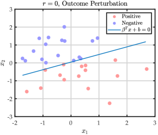
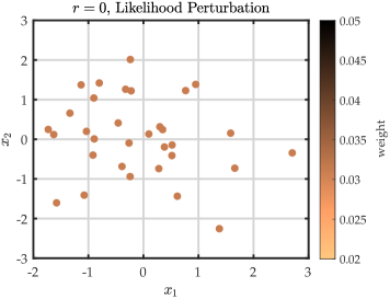
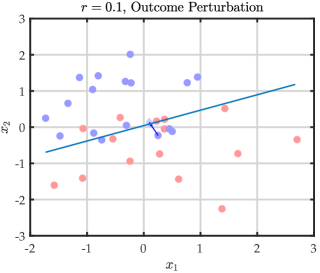
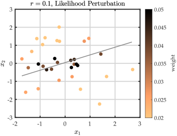
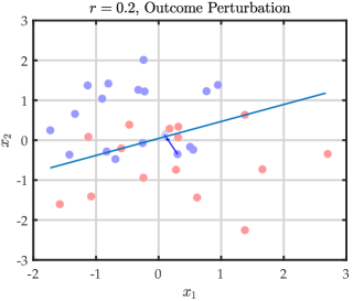
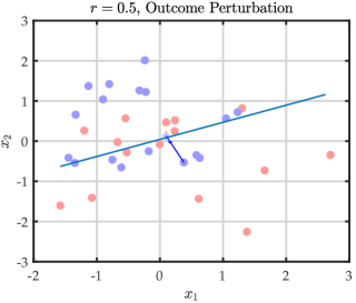
Figure 1: Decision boundary and worst-case distribution.

6 Visualization of the Worst-Case Distribution

We visualize the worst-case distribution obtained by solving the problem (2) when the cost function is as in (19) in the context of supervised learning to provide a better understanding of the perturbations on the actual outcomes and likelihood ratios.

Support vector machine (SVM). We consider binary classification, in which the data points are given by $\{\hat{v}_{i}=(\hat{x}_{i},\hat{y}_{i})\}_{i=1}^{n}$ with feature vectors $\hat{x}_{i}\in\mathbb{R}^{2}$ and labels $\hat{y}_{i}\in\{+1,-1\}$. For SVM, the loss function is the Hinge loss, that is, $\ell_{(\beta,b)}((x,y))=\max\{1-y\cdot(\beta^{\top}x+b),0\}$. To be specific, we choose the cost function $d$ in (19) as $d(v,\hat{v})=\|x-\hat{x}\|^{2}+\infty\cdot|y-\hat{y}|$ and $\theta_{1}=\theta_{2}=1$.

We sample $\beta^{\star}\in\mathbb{R}^{2}$ from the multivariate standard normal distribution. Then, we generate 32 training samples $X\in\mathbb{R}^{2}$ drawn from the standard multivariate normal distribution. For each sample, we construct pseudo-labels $\tilde{y}$ such that $\tilde{y}=1$ if $\langle\beta^{\star},x\rangle\geqslant 0$ and $\tilde{y}=-1$ otherwise. Then, we construct label $y$ for each sample $x$ as $y=1$ if  $\tilde{y}+\tilde{\omega}\geqslant 0$ and $y=-1$ otherwise, where $\tilde{\omega}\sim\mathcal{N}(0,10^{-4})$. Next, we train empirical support vector machine on the training samples and obtain $\hat{\beta}\in\mathbb{R}^{2}$ and $\hat{b}\in\mathbb{R}$. For $r\in\{0,0.1,0.2,0.5\}$, we solve the worst-case risk problem in (2) with $\ell_{(\hat{\beta},\hat{b})}$, which admits a finite convex program reformulation thanks to Corollary 1. Then, we construct the worst-case distribution $\pi^{\star}_{((X,Y),W)}=n^{-1}\sum_{i=1}^{n}\delta_{((x^{\star},y^{\star}),w^{\star})}$. Note that by construction of the cost function $d$, we have $y_{i}^{\star}=\hat{y}_{i}$ for all $i\in[n]$, that is, in the adversarial distribution the label of each sample cannot be perturbed.

The plots in the left column of Figure 1 show the data points located at $\{x_{i}^{\star}\}_{i=1}^{n}$, where $x_{i}^{\star}=({x_{i_{1}}}^{\star},{x_{i_{2}}}^{\star})$ and the color of data points represent the label $\{y_{i}^{\star}\}_{i=1}^{n}$. The boundary indicated by the blue line is obtained by $\hat{\beta}x+\hat{b}$. The plots in the right column of Figure 1 illustrate the weight $\{w_{i}^{\star}\}_{i=1}^{n}$ on each atom $\hat{x}_{i}$ in the worst-case distribution and the color map on the right of each plot show the values of $\hat{w}_{i}$. From top to bottom of Figure 1 the radius $r$ increases. Notably, as $r$ increases we observe an increase in the number of missclassified data points in the worst-case distribution. Additionally, the worst-case distribution assigns higher weights $w_{i}^{\star}$ to data points that are farther away from the correct side.

7 Closing Remarks

Our paper presents a novel approach that integrates divergence-based and Wasserstein-based DRO within a unified framework based on optimal transport. By leveraging the power of OT with conditional moment constraints, we provide a transparent way to simultaneously consider both likelihood and outcome misspecification in our uncertainty sets. The strong duality results and tractable reformulations we introduce enhance the practicality of our unified approach, making it highly applicable to a wide range of real-world scenarios. Furthermore, by leveraging the rich tools in OT, we believe our work opens up new avenues and flexible research paradigms in the DRO community.

Appendix A Technical Lemmas

Lemma 2 (Sion’s minimax theorem, [Sion,, 1958]).

Let $\mathcal{X}$ be a compact convex subset of a linear topological space and $\mathcal{Y}$ a convex subset of a linear topological space. If $f$ is a real-valued function on $\mathcal{X}\times Y$ with

1. $f(x,\cdot)$ lower semicontinuous and quasi-convex on $\mathcal{Y}$, $\forall x\in\mathcal{X}$.

2. $f(\cdot,y)$ upper semicontinuous and quasi-concave on $\mathcal{X}$, $\forall y\in\mathcal{Y}$.
   Then,

   $$\max_{x\in\mathcal{X}}\inf_{y\in\mathcal{Y}}f(x,y)=\inf_{y\in\mathcal{Y}}\max_{x\in\mathcal{X}}f(x,y).$$

Lemma 3.

Problem (2) can be equivalently written as

$$\begin{array}[]{cclll}&\sup&\mathbb{E}_{\pi}[f(V,W)]\\ &\operatorname{\textrm{s.t.}}2&\pi\in\mathcal{P}((\mathcal{V}\times\mathcal{W})\times(\mathcal{V}\times\mathcal{W}))\\ &&\pi_{(\hat{V},\hat{W})}=\hat{\nu}\\ &&\mathbb{E}_{\pi}[W|\mathcal{G}]=1\quad\pi\text{-a.s.}\\ &&\mathbb{E}_{\pi}[c((V,W),(\hat{V},\hat{W}))]\leqslant r.\end{array}$$

Proof.

By exploiting Definition 1, we can equivalently reformulate problem (2) as

$$\begin{array}[]{cclll}&\sup&\mathbb{E}_{\nu}[f(V,W)]\\ &\operatorname{\textrm{s.t.}}2&\inf\limits_{\nu\in\Pi_{M}(\nu,\hat{\nu})}\mathbb{E}_{\pi}[c((V,W),(\hat{V},\hat{W}))]\leqslant r.\end{array}$$ (37)

For any given probability measures $\nu$ and $\hat{\nu}$, the set $\Pi_{M}(\nu,\hat{\nu})$ is defined as

$$\Pi_{M}(\nu,\hat{\nu})\!=\!\{\pi\!\in\!\mathcal{P}((\mathcal{V}\times\mathcal{W})\times(\mathcal{V}\times\mathcal{W})):\pi_{(V,W)}\!=\!\nu,\pi_{(\hat{V},\hat{W})}\!=\!\hat{\nu},\mathbb{E}_{\pi}[W|\mathcal{G}]=1,\pi\text{-a.s.}\},$$

which is tight in $\mathcal{P}((\mathcal{V}\times\mathcal{W})\times(\mathcal{V}\times\mathcal{W}))$ by [Villani,, 2009, Lemma 4.4]. Then, Prokhorov’s theorem ensures that $\Pi_{M}(\nu,\hat{\nu})$ is compact. As $c$ is lower semicontinuous, we can invoke [Villani,, 2009, Theorem 4.1], and conclude that the infimum over $\pi\in\Pi_{M}(\nu,\hat{\nu})$ is attained, which allows us to remove the infimum operator on the left-hand side of the inequality constraint above and to treat the transportation plan $\pi$ as a decision variable in the overall maximization problem. Hence, we can equivalently reformulate problem (37) as

$$\begin{array}[]{cclll}&\sup&\mathbb{E}_{\nu}[f(V,W)]\\ &\operatorname{\textrm{s.t.}}2&\mathbb{E}_{\pi}[c((V,W),(\hat{V},\hat{W}))]\leqslant r\\ &&\pi_{(V,W)}=\nu,\pi_{(\hat{V},\hat{W})}=\hat{\nu}\\ &&\mathbb{E}_{\pi}[W|\mathcal{G}]=1\quad\pi\text{-a.s.}\end{array}$$

As $\nu$ is the marginal distribution of $(V,W)$ under any transportation plan $\pi\in\Pi_{M}(\nu,\hat{\nu})$, we can thus reformulate the above optimization as (3) without using $\nu$. Hence, the claim follows. ∎

References

• Ali and Silvey, [1966] Ali, S. M. and Silvey, S. D. (1966). A general class of coefficients of divergence of one distribution from another. Journal of the Royal Statistical Society: Series B (Methodological), 28(1):131–142.
• An and Gao, [2021] An, Y. and Gao, R. (2021). Generalization bounds for (Wasserstein) robust optimization. In Advances in Neural Information Processing Systems 34.
• Aolaritei et al., [2022] Aolaritei, L., Shafieezadeh-Abadeh, S., and Dörfler, F. (2022). The performance of Wasserstein distributionally robust m-estimators in high dimensions. arXiv:2206.13269.
• Arjovsky et al., [2017] Arjovsky, M., Chintala, S., and Bottou, L. (2017). Wasserstein generative adversarial networks. In International conference on machine learning, pages 214–223. PMLR.
• Azizian et al., [2022] Azizian, W., Iutzeler, F., and Malick, J. (2022). Regularization for Wasserstein distributionally robust optimization. arXiv:2205.08826.
• Azizian et al., [2023] Azizian, W., Iutzeler, F., and Malick, J. (2023). Exact generalization guarantees for (regularized) Wasserstein distributionally robust models. arXiv:2305.17076.
• [7] Bayraksan, G. and Love, D. K. (2015a). Data-driven stochastic programming using phi-divergences. In The operations research revolution, pages 1–19. INFORMS.
• [8] Bayraksan, G. and Love, D. K. (2015b). Data-driven stochastic programming using phi-divergences. In The Operations Research Revolution, pages 1–19.
• Beiglböck et al., [2013] Beiglböck, M., Henry-Labordere, P., and Penkner, F. (2013). Model-independent bounds for option prices-a mass transport approach. Finance and Stochastics, 17(3):477–501.
• Beiglböck et al., [2017] Beiglböck, M., Nutz, M., and Touzi, N. (2017). Complete duality for martinagle optimal transport on the line. The Annals of Probability, 45(5):3038–3074.
• Ben-Tal et al., [2009] Ben-Tal, A., El Ghaoui, L., and Nemirovski, A. (2009). Robust Optimization, volume 28. Princeton university press.
• Bennouna and Van Parys, [2022] Bennouna, A. and Van Parys, B. (2022). Holistic robust data-driven decisions. arXiv:2207.09560.
• Bertsimas et al., [2018] Bertsimas, D., Gupta, V., and Kallus, N. (2018). Data-driven robust optimization. Mathematical Programming, 167:235–292.
• Bertsimas and Sim, [2004] Bertsimas, D. and Sim, M. (2004). The price of robustness. Operations research, 52(1):35–53.
• Blanchet et al., [2019] Blanchet, J., Kang, Y., and Murthy, K. (2019). Robust Wasserstein profile inference and applications to machine learning. Journal of Applied Probability, 56(3):830–857.
• Blanchet and Murthy, [2019] Blanchet, J. and Murthy, K. (2019). Quantifying distributional model risk via optimal transport. Mathematics of Operations Research, 44(2):565–600.
• [17] Blanchet, J., Murthy, K., and Nguyen, V. A. (2021a). Statistical analysis of Wasserstein distributionally robust estimators. In Tutorials in Operations Research: Emerging Optimization Methods and Modeling Techniques with Applications, pages 227–254. INFORMS.
• Blanchet et al., [2022] Blanchet, J., Murthy, K., and Si, N. (2022). Confidence regions in Wasserstein distributionally robust estimation. Biometrika, 109(2):295–315.
• [19] Blanchet, J., Murthy, K., and Zhang, F. (2021b). Optimal transport-based distributionally robust optimization: Structural properties and iterative schemes. Mathematics of Operations Research.
• Blanchet and Shapiro, [2023] Blanchet, J. and Shapiro, A. (2023). Statistical limit theorems in distributionally robust optimization. arXiv:2303.14867.
• Blanchet and Si, [2019] Blanchet, J. and Si, N. (2019). Optimal uncertainty size in distributionally robust inverse covariance estimation. Operations Research Letters, 47(6):618–621.
• Breuer and Csiszár, [2016] Breuer, T. and Csiszár, I. (2016). Measuring distribution model risk. Mathematical Finance, 26(2):395–411.
• Chen and Paschalidis, [2018] Chen, R. and Paschalidis, I. C. (2018). A robust learning approach for regression models based on distributionally robust optimization. Journal of Machine Learning Research, 19(13).
• Chen et al., [2020] Chen, R., Paschalidis, I. C., et al. (2020). Distributionally robust learning. Foundations and Trends® in Optimization, 4(1-2):1–243.
• Chen et al., [2022] Chen, Z., Kuhn, D., and Wiesemann, W. (2022). Data-driven chance constrained programs over Wasserstein balls. Operations Research.
• Cranko et al., [2021] Cranko, Z., Shi, Z., Zhang, X., Nock, R., and Kornblith, S. (2021). Generalised Lipschitz regularisation equals distributional robustness. In International Conference on Machine Learning, pages 2178–2188. PMLR.
• Csiszár, [1964] Csiszár, I. (1964). Eine informationstheoretische ungleichung und ihre anwendung auf beweis der ergodizitaet von markoffschen ketten. Magyer Tud. Akad. Mat. Kutato Int. Koezl., 8:85–108.
• Csiszar, [1967] Csiszar, I. (1967). Information-type measures of difference of probability distributions and indirect observation. Studia Scientiarum Mathematicarum Hungarica, 2:229–318.
• Cuturi, [2013] Cuturi, M. (2013). Sinkhorn distances: Lightspeed computation of optimal transport. In Advances in neural information processing systems 26.
• Dapogny et al., [2022] Dapogny, C., Iutzeler, F., Meda, A., and Thibert, B. (2022). Entropy-regularized Wasserstein distributionally robust shape and topology optimization. arXiv:2209.01500.
• Dolinsky and Soner, [2014] Dolinsky, Y. and Soner, H. M. (2014). Martingale optimal transport and robust hedging in continuous time. Probability Theory and Related Fields, 160(1):391–427.
• Duchi and Namkoong, [2021] Duchi, J. C. and Namkoong, H. (2021). Learning models with uniform performance via distributionally robust optimization. The Annals of Statistics, 49(3):1378–1406.
• El Ghaoui and Nilim, [2005] El Ghaoui, L. and Nilim, A. (2005). Robust solutions to markov decision problems with uncertain transition matrices. Operations Research, 53(5):780–798.
• Gao, [2022] Gao, R. (2022). Finite-sample guarantees for Wasserstein distributionally robust optimization: Breaking the curse of dimensionality. Operations Research.
• Gao et al., [2022] Gao, R., Chen, X., and Kleywegt, A. J. (2022). Wasserstein distributionally robust optimization and variation regularization. Operations Research.
• [36] Gao, R. and Kleywegt, A. (2022a). Distributionally robust stochastic optimization with Wasserstein distance. Mathematics of Operations Research.
• [37] Gao, R. and Kleywegt, A. (2022b). Distributionally robust stochastic optimization with Wasserstein distance. Mathematics of Operations Research.
• Genevay et al., [2016] Genevay, A., Cuturi, M., Peyré, G., and Bach, F. (2016). Stochastic optimization for large-scale optimal transport. In Advances in neural information processing systems 29.
• Gulrajani et al., [2017] Gulrajani, I., Ahmed, F., Arjovsky, M., Dumoulin, V., and Courville, A. C. (2017). Improved training of Wasserstein gans. Advances in neural information processing systems, 30.
• Hansen and Sargent, [2001] Hansen, L. P. and Sargent, T. J. (2001). Robust control and model uncertainty. American Economic Review, 91(2):60–66.
• He and Lam, [2021] He, S. and Lam, H. (2021). Higher-order expansion and bartlett correctability of distributionally robust optimization. arXiv:2108.05908.
• Hu and Hong, [2013] Hu, Z. and Hong, L. J. (2013). Kullback-leibler divergence constrained distributionally robust optimization. Available at Optimization Online, 1(2):9.
• Iyengar, [2005] Iyengar, G. N. (2005). Robust dynamic programming. Mathematics of Operations Research, 30(2):257–280.
• Jiang and Guan, [2018] Jiang, R. and Guan, Y. (2018). Risk-averse two-stage stochastic program with distributional ambiguity. Operations Research, 66(5):1390–1405.
• Kuhn et al., [2019] Kuhn, D., Esfahani, P. M., Nguyen, V. A., and Shafieezadeh-Abadeh, S. (2019). Wasserstein distributionally robust optimization: Theory and applications in machine learning. In Operations research & management science in the age of analytics, pages 130–166. Informs.
• Lam, [2016] Lam, H. (2016). Robust sensitivity analysis for stochastic systems. Mathematics of Operations Research, 41(4):1248–1275.
• Lam, [2019] Lam, H. (2019). Recovering best statistical guarantees via the empirical divergence-based distributionally robust optimization. Operations Research, 67(4):1090–1105.
• Lee and Raginsky, [2018] Lee, J. and Raginsky, M. (2018). Minimax statistical learning with Wasserstein distances. Advances in Neural Information Processing Systems, 31.
• Li, [2021] Li, J. (2021). Efficient and Provable Algorithms for Wasserstein Distributionally Robust Optimization in Machine Learning. PhD thesis, The Chinese University of Hong Kong (Hong Kong).
• Li et al., [2020] Li, J., Chen, C., and So, A. M.-C. (2020). Fast epigraphical projection-based incremental algorithms for Wasserstein distributionally robust support vector machine. In Advances in Neural Information Processing Systems 33, pages 4029–4039.
• Li et al., [2019] Li, J., Huang, S., and So, A. M.-C. (2019). A first-order algorithmic framework for distributionally robust logistic regression. In Advances in Neural Information Processing Systems 32.
• Li et al., [2022] Li, J., Lin, S., Blanchet, J., and Nguyen, V. A. (2022). Tikhonov regularization is optimal transport robust under martingale constraints. In Advances in Neural Information Processing Systems 35.
• Lim et al., [2006] Lim, A. E., Shanthikumar, J. G., and Shen, Z. M. (2006). Model uncertainty, robust optimization, and learning. In Models, Methods, and Applications for Innovative Decision Making, pages 66–94. INFORMS.
• Lin et al., [2022] Lin, F., Fang, X., and Gao, Z. (2022). Distributionally robust optimization: A review on theory and applications. Numerical Algebra, Control and Optimization, 12(1):159–212.
• Liu et al., [2023] Liu, Z., Van Parys, B. P., and Lam, H. (2023). Smoothed $f$-divergence distributionally robust optimization: Exponential rate efficiency and complexity-free calibration. arXiv:2306.14041.
• Mohajerin Esfahani and Kuhn, [2018] Mohajerin Esfahani, P. and Kuhn, D. (2018). Data-driven distributionally robust optimization using the Wasserstein metric: Performance guarantees and tractable reformulations. Mathematical Programming, 171(1):115–166.
• Namkoong and Duchi, [2016] Namkoong, H. and Duchi, J. C. (2016). Stochastic gradient methods for distributionally robust optimization with f-divergences. Advances in neural information processing systems, 29.
• Namkoong and Duchi, [2017] Namkoong, H. and Duchi, J. C. (2017). Variance-based regularization with convex objectives. Advances in Neural Information Processing Systems, 30.
• Peyré et al., [2019] Peyré, G., Cuturi, M., et al. (2019). Computational optimal transport: With applications to data science. Foundations and Trends® in Machine Learning, 11(5-6):355–607.
• Pflug and Wozabal, [2007] Pflug, G. and Wozabal, D. (2007). Ambiguity in portfolio selection. Quantitative Finance, 7(4):435–442.
• Rahimian and Mehrotra, [2022] Rahimian, H. and Mehrotra, S. (2022). Frameworks and Results in Distributionally Robust Optimization. Open Journal of Mathematical Optimization.
• Sason, [2018] Sason, I. (2018). On f-divergences: Integral representations, local behavior, and inequalities. Entropy, 20(5):383.
• Scarf, [1958] Scarf, H. (1958). A min-max solution of an inventory problem in studies in the mathematical theory of inventory and production.(k. arrow, s. karlin and h. scarf, eds.) 201-209.
• Seguy et al., [2018] Seguy, V., Damodaran, B. B., Flamary, R., Courty, N., Rolet, A., and Blondel, M. (2018). Large scale optimal transport and mapping estimation. In International Conference on Learning Representations.
• Shafieezadeh-Abadeh et al., [2023] Shafieezadeh-Abadeh, S., Aolaritei, L., Dörfler, F., and Kuhn, D. (2023). New perspectives on regularization and computation in optimal transport-based distributionally robust optimization. arXiv:2303.03900.
• Shafieezadeh-Abadeh et al., [2019] Shafieezadeh-Abadeh, S., Kuhn, D., and Esfahani, P. M. (2019). Regularization via mass transportation. Journal of Machine Learning Research, 20(103):1–68.
• Shafieezadeh Abadeh et al., [2015] Shafieezadeh Abadeh, S., Mohajerin Esfahani, P. M., and Kuhn, D. (2015). Distributionally robust logistic regression. Advances in Neural Information Processing Systems, 28.
• Shapiro, [2001] Shapiro, A. (2001). On duality theory of conic linear problems. In Semi-infinite programming, pages 135–165. Springer.
• Sinha et al., [2018] Sinha, A., Namkoong, H., and Duchi, J. (2018). Certifying some distributional robustness with principled adversarial training. In International Conference on Learning Representations.
• Sion, [1958] Sion, M. (1958). On general minimax theorems. Pacific Journal of Mathematics, 8(1):171–176.
• Taşkesen et al., [2023] Taşkesen, B., Shafieezadeh-Abadeh, S., and Kuhn, D. (2023). Semi-discrete optimal transport: Hardness, regularization and numerical solution. Mathematical Programming, 199(1-2):1033–1106.
• Van der Vaart, [2000] Van der Vaart, A. W. (2000). Asymptotic statistics, volume 3. Cambridge university press.
• Van Parys et al., [2021] Van Parys, B. P., Esfahani, P. M., and Kuhn, D. (2021). From data to decisions: Distributionally robust optimization is optimal. Management Science, 67(6):3387–3402.
• Villani, [2009] Villani, C. (2009). Optimal transport: old and new, volume 338. Springer.
• Wang et al., [2021] Wang, J., Gao, R., and Xie, Y. (2021). Sinkhorn distributionally robust optimization. arXiv:2109.11926.
• Wang et al., [2016] Wang, Z., Glynn, P. W., and Ye, Y. (2016). Likelihood robust optimization for data-driven problems. Computational Management Science, 13:241–261.
• Wozabal, [2012] Wozabal, D. (2012). A framework for optimization under ambiguity. Annals of Operations Research, 193(1):21–47.
• Xie, [2021] Xie, W. (2021). On distributionally robust chance constrained programs with Wasserstein distance. Mathematical Programming, 186(1-2):115–155.
• Yu et al., [2022] Yu, Y., Lin, T., Mazumdar, E. V., and Jordan, M. (2022). Fast distributionally robust learning with variance-reduced min-max optimization. In International Conference on Artificial Intelligence and Statistics, pages 1219–1250. PMLR.
• Yue et al., [2021] Yue, M.-C., Kuhn, D., and Wiesemann, W. (2021). On linear optimization over Wasserstein balls. Mathematical Programming, pages 1–16.
• [81] Zhang, L., Yang, J., and Gao, R. (2022a). A simple and general duality proof for Wasserstein distributionally robust optimization. arXiv:2205.00362.
• [82] Zhang, X., Blanchet, J., Marzouk, Y., Nguyen, V. A., and Wang, S. (2022b). Wasserstein distributionally robust gaussian process regression and linear inverse problems. arXiv:2205.13111.
• Zhao and Guan, [2018] Zhao, C. and Guan, Y. (2018). Data-driven risk-averse stochastic optimization with Wasserstein metric. Operations Research Letters, 46(2):262–267.