Large black hole entropy from the giant brane expansion

Abstract

We show that the Bekenstein-Hawking entropy of large supersymmetric black holes in AdS${}_{5}\times S^{5}$ emerges from remarkable cancellations in the giant graviton expansions recently proposed by Imamura, and Gaiotto and Lee, independently. A similar cancellation mechanism is shown to happen in the exact expansion in terms of free fermions recently put-forward by Murthy. These two representations can be understood as sums over independent systems of giant D3-branes and free fermions, respectively. At large charges, the free energy of each independent system localizes to its asymptotic expansion near the leading singularity. The sum over the independent systems maps their localized free energy to the localized free energy of the superconformal index of $U(N)$ $\mathcal{N}=4$ SYM. This result constitutes a non-perturbative test of the giant graviton expansion valid at any value of $N$.

1 Introduction

Recently, the counting of small $\frac{1}{16}$-BPS states in $4d$ $U(N)$ $\mathcal{N}=4$ SYM on $\mathbb{R}\times S^{3}$ Kinney:2005ej ; Romelsberger:2005eg has been nicely related to the problem of counting graviton and giant graviton BPS excitations in $AdS_{5}\times S^{5}\,$ Imamura:2021ytr ; Arai:2019xmp  Gaiotto:2021xce ; Lee:2022vig . It is known that upon truncation to charges of order $N$ or smaller, the $\frac{1}{16}$-BPS index $\mathcal{I}(q)\,$ matches the truncation of the index $\mathcal{I}_{KK}(q)$ of a gas of gravitons in $AdS_{5}\times S^{5}\,$. This match happens at any value of the gauge rank $N\,$.

The index counting multigravitons $\mathcal{I}_{KK}(q)$ is independent of the gauge rank $N$ Kinney:2005ej . The $N$-dependence of the complete index $\mathcal{I}(q)\,$ appears when it is truncated at powers of order $N\,$ or larger Murthy:2020rbd ; Agarwal:2020zwm . These $N$-dependent contributions can be always reorganized in linear combinations of subsums with overall weights $q^{nN}$ , where $n$ is a non-negative integer. As recognized in  Imamura:2021ytr ; Arai:2019xmp  Gaiotto:2021xce ; Lee:2022vig , there is at least one such reorganization for which the $q^{nN}$-weighted subsums correspond to truncated indices of $n$ D3 brane excitations wrapping supersymmetric and contractible $S^{3}$-cycles in $S^{5}\,$. However, such reorganization is obviously non-unique. 

Whether this correspondence holds for the complete $q$-series $\mathcal{I}(q)$ or it is just a property of its truncation at certain order of charges remains an open question.  For example, it is plausible that new stringy excitations in $AdS_{5}\times S^{5}$ are required at large enough $N$ and charges of order $N^{2}$ in order to keep the correspondence going. For such charges the number of $\frac{1}{16}$-BPS gauge-invariant states in the gauge theory grows as the exponential of the Bekenstein Hawking entropy of the dual BPS black holes Cabo-Bizet:2018ehj ; Choi:2018hmj ; Benini:2018ywd . Thus, in a sense, it is a priori unclear whether such an entropy growth can be understood by working solely within the D3 brane systems prescribed by the proposal of Imamura:2021ytr .

Another giant graviton-like reorganization of the index, an exact one by construction, has been recently put forward in Murthy:2022ien .  This reorganization is not quite the same as the proposal of Imamura:2021ytr – as explained in Liu:2022olj – but it seems to be closely related to it as argued in Murthy:2022ien and Eniceicu:2023uvd . Being an exact expansion, it would be useful to understand the physics behind it and how close it is to the physics of the proposals of Imamura:2021ytr and Gaiotto:2021xce . 

The main goal of this paper is to study the giant graviton representations of Imamura:2021ytr ; Gaiotto:2021xce ; Lee:2022vig and Murthy:2022ien at large charges and to compare the results with the ones obtained with the canonical matrix integral representation Choi:2018hmj ; Honda:2019cio ; ArabiArdehali:2019tdm ; Kim:2019yrz ; Cabo-Bizet:2019osg ; Cassani:2021fyv .

Using the representation of Imamura:2021ytr and working in the macrocanonical ensemble, we will show that an exponentially large number of cancellations occurs when summing over individual giant graviton contributions at large charges and for all $N\,$. Such cancellations can be explained in terms of an extremization mechanism for the giant graviton number $n\,$. At $N\,\gg\,1$ this mechanism explains how the dual black-hole entropy is recovered within the giant graviton expansion, and its derivation provides, in particular, a first-principle explanation of the large-$N$ extremization mechanism proposed in Choi:2022ovw . More generally, the mechanism here identified implies that the latter cancellations continue to happen at large charges for any value of $N\,$, not just in the large-$N$ expansion. It will be also shown that a similar extremization mechanism holds for the exact giant graviton-like representation of Murthy:2022ien and checked – against numerics – how such mechanism exactly accounts for the exponentially large cancellations happening after summing over individual giant graviton-like subseries (in appendix D, see plot 1).

In the representation of Imamura:2021ytr ; Gaiotto:2021xce ; Lee:2022vig , this extremization mechanism will tell us that the black hole entropy Gutowski:2004ez ; Gutowski:2004yv ; Cvetic:2004ny comes from the superposition of a pair of complex conjugated saddle points whose semiclassical contributions evaluate the sum over giant graviton brane number $n$. The canonical matrix integral representation of the index Kinney:2005ej is known to be dominated by a pair of complex conjugated eigenvalue configurations too Cabo-Bizet:2020ewf ; Benini:2018ywd ; Cabo-Bizet:2019eaf ; Cabo-Bizet:2020nkr ; Aharony:2021zkr Agarwal:2020zwm . The latter and the former pairs are related: they provide two different interpretations of the very same contributions to the index at large charges of order $N^{2}$.  It remains for the future to understand the physics of the excitations accounting for subleading corrections in both, the canonical matrix model and giant graviton(-like) expansions, and for both small and large black holes.   

The paper is organized as follows. After a summary of results, in section 2 we explain how the large-charge approximation simplifies the counting of states, and introduce tools that will be useful later on. In section 3 we introduce conventions, and the two representations of the superconformal index that we will study. In section 3.3, and as warm-up for the analysis of the giant graviton indices, we compute the large charge asymptotics of the superconformal index using a novel approach that turns out to be convenient for our scope. In section 4 we apply the previously mentioned asymptotic tools to understand how the large-charge growth of the index is matched by the large-charge counting of giant gravitons for all $N\,$ not just at $N\gg 1\,$.  In appendix C we explain the role played by the choice of contour of integration Lee:2022vig Beccaria:2023zjw in the large charge expansion. In appendix D we move on to answer the very same question from the exact representation of the superconformal index put-forward in Murthy:2022ien and conclude explaining how exponentially large cancellations among individual giant graviton-like contributions are understood in the macrocanonical ensemble.

1.1 Summary of main results

Let us briefly summarize our main results. Detailed expositions will be presented in the main body of the paper.

As mentioned in the introduction, the authors of Imamura:2021ytr ; Gaiotto:2021xce ; Lee:2022vig proposed that the superconformal index $\mathcal{I}$ of four-dimensional $U(N)$ $\mathcal{N}=4$ SYM on $S^{3}$ can be expanded in a sum over indices $\mathcal{I}_{\underline{n}}:=\mathcal{I}_{KK}\,\mathcal{I}_{n_{1},n_{2},n_{3}}$ of stacks of $n_{1}$, $n_{2}$, $n_{3}$ giant graviton D3-branes wrapping three contractible $S^{3}$-cycles in $S^{5}\,$.  The details of this proposal will be given in subsection 3.1. Schematically, it looks as follows

$$\mathcal{I}(\tau)\,\underset{?}{=}\,\sum_{n_{1},n_{2},n_{3}}\mathcal{I}_{\underline{n}}(\tau)\,,$$ (1)

where

$$\mathcal{I}(\tau)\underset{?}{=}\sum_{Q\,\in\,\mathcal{S}_{\mathcal{N}=4}}\,a(Q)e^{2\pi{\rm i}\tau Q}\,,\qquad\mathcal{I}_{\underline{n}}(\tau)=\sum_{Q_{gg}\,\in\,\mathcal{S}_{gg}}\,a_{\underline{n}}(Q_{gg})e^{2\pi{\rm i}\tau Q_{gg}}\,.$$ (2)

The letter $\tau$ denotes the set of chemical potentials $\{\varphi_{1},\varphi_{2},\varphi_{3},\ldots\}$ dual to the conserved global charges – including spin $J$ and $R$-charges – whose individual eigenvalues in both $\mathcal{N}=4$ and the infinitely many stacks of giant graviton branes  will be denoted by the letters $Q\,$ and $Q_{gg}$, respectively. $\mathcal{S}_{\mathcal{N}=4}$ and $\mathcal{S}_{gg}\,$, are the respective charge-lattices. These two lattices are very different and in consequence the domains of convergence of the Hamiltonian traces that define $\mathcal{I}(\tau)$ and $\mathcal{I}_{n_{1},n_{2},n_{3}}(\tau)$ are different. Thus, to check (1), analytic continuation in $\tau$ is necessary, either in the left or right-hand side.

The microcanonical version of the proposal (1) is

$$\sum_{\underline{n}}a_{\underline{n}}(Q_{gg})\,\underset{?}{=}\,\begin{cases}a(Q)\,,\quad\text{if}\quad Q_{gg}\,\in\,\mathcal{S}_{\mathcal{N}=4}\\ \,0\,,\qquad\,\quad\text{otherwise}\end{cases}\,.$$ (3)

For later convenience it should be said that the sum over $\underline{n}$ in (3) is not really a series because $a_{\underline{n}}(Q_{gg})$ vanishes for large enough values $\underline{n}\,$, at a fixed $Q_{gg}\,$.  (3) says that the sum over giant graviton numbers $\underline{n}$ must project the BPS giant graviton spectrum $\mathcal{S}_{gg}$ to the much smaller gauge-theory spectrum $\mathcal{S}_{\mathcal{N}=4}\,$. As said before, the proposal (3) has been checked for small enough values of $Q\sim N$ Imamura:2021ytr Lee:2022vig .

Our goal is to show that at large charges $Q\to\infty$ (and for all $N$) a precise version of the following asymptotic relation holds 

$$\sum_{\underline{n}}\,a_{\underline{n}}(Q)\,\sim\,a(Q)\,\sim\,e^{\left(\sqrt{3}\right)3^{1/3}\pi\,c\,\,{J^{2/3}}{N^{2/3}}}\,,$$ (4)

meaning that at large charges and for all $N$ the sum over the giant graviton microcanonical indices matches the exponential growth of $\frac{1}{16}$-BPS states. In this relation the quantity $c$ is an order $1$ real contribution that depends on how fast the spin $J$ grows in relation to the $R$-charges, we will come back to comment on it below (e.g. a particularly simple case where $c$ is simply a c-number will be reported in (LABEL:eq:AsymptoticsLargeSpin)).

Let us briefly explain how (4) will be obtained. In subsection 2.3 we will introduce a large-charge localization Lemma that will help us to compute localized contributions $a^{loc}_{\pm,\underline{n}}$ to the giant graviton index. If we define the microcanonical index of giant gravitons to be

$$a_{\underline{n}}(Q):=\int_{\Gamma}d\tau\,\mathcal{I}_{\underline{n}}(\tau)\,e^{-2\pi{\rm i}\tau Q}\,,$$ (5)

with $\Gamma$ being a period of the integrand, the $a^{loc}_{\pm,\underline{n}}$ are two equally-dominating contributions to (5) in its asymptotic expansion at large $R$-charges, fixed $J\,$, and fixed $\underline{n}\,$

$$a_{\underline{n}}(Q)\,\sim\,a^{loc}_{+,\underline{n}}(Q)+a^{loc}_{-,\underline{n}}(Q)\,.$$ (6)

These two contributions $\pm$ are complex conjugated to each other

$$a^{loc}_{\pm,\underline{n}}(Q)=\int_{\Gamma_{\pm}}d\tau\,\mathcal{I}^{(\pm)}_{\underline{n}}(\tau)\,e^{-2\pi{\rm i}\tau Q}\,.$$ (7)

The large-charge localization Lemma of 2.3 will tell us that the contours $\Gamma_{\pm}$ can be understood as small subpieces of the contour $\Gamma\,$, centered at the leading (exponential) divergencies of $\mathcal{I}_{\underline{n}}(\tau)\,$. The latter divergencies of $\mathcal{I}_{\underline{n}}(\tau)$ are in the subset of chemical potentials $\underline{\varphi}=\{\varphi_{1},\varphi_{2},\varphi_{3}\}$ dual to $R$-charges. In the cases of interest to us, there are two types of such divergences that we label by the two choices of signs $\pm\,$. The localized integrands $\mathcal{I}^{(\pm)}_{\underline{n}}(\tau)$ are the leading asymptotic expansions of $\mathcal{I}_{\underline{n}}(\tau)$ around the divergencies $\pm$ and are exact in the chemical potentials $\tau$ that are not $\varphi$’s.

After commuting the sum over $n$ with the integrals over $\tau$ in (5) one obtains

$$\sum_{\underline{n}}a^{loc}_{\pm,\underline{n}}(Q)=\int_{\Gamma_{\pm}}d\tau\,\Bigl{(}\sum_{\underline{n}}\mathcal{I}^{\pm}_{\underline{n}}(\tau)\Bigr{)}\,e^{-2\pi{\rm i}\tau Q}\,.$$ (8)

As it will be explained in the main body of the paper, the sum over $\underline{n}\,$ can be replaced by an integral over a compact domain whose asymptotic behaviour around the singularities $\pm$ (and at large $R$-charges) can be obtained by the saddle point method

$$\sum_{\underline{n}}\mathcal{I}^{(\pm)}_{\underline{n}}(\tau)\,\sim\,\mathcal{I}^{(\pm)}_{\underline{n}^{\star}}(\tau)\,.$$ (9)

The saddle point condition ends up taking a simple linear form that fixes $n=\underline{n}^{\star}:=\underline{n}^{\star}(\tau)\,$ as a function of $\tau$. The function $n^{\star}(\tau)$ is defined by a linear relation of the schematic form

$$\underline{\varphi}\,\cdot\,\underline{\underline{n}}^{\star}_{\pm}\,=\frac{N}{\tau^{2}}f_{\pm}(\tau)\,,$$ (10)

where $f_{\pm}(\tau)$ are cubic polynomials in $\tau$ such that $|f_{\pm}(0)|$ is finite and non zero. The explicit form of this equation will be specified in the main body of the paper. 

To compute the asymptotic behaviour of  $\int_{\Gamma_{\pm}}d\tau\,\mathcal{I}^{(\pm)}_{\underline{n}^{\star}_{\pm}}(\tau)e^{-2\pi{\rm i}\tau Q}$ at large $Q$, not just at large $R$-charges as before, but also at large spin $J\,$, we use again a saddle point evaluation

$$\int_{\Gamma_{\pm}}d\tau\,\mathcal{I}^{(\pm)}_{\underline{n}^{\star}_{\pm}}(\tau)e^{-2\pi{\rm i}\tau Q}\,\sim\,\mathcal{I}^{(\pm)}_{\underline{n}^{\star}_{\pm}}(\tau)e^{-2\pi{\rm i}\tau Q}\,=:\,a^{loc}_{\pm,\underline{n}^{\star}_{\pm}}\,.$$ (11)

This time the saddle-point condition fixes the $\tau$’s as a function of $Q$, for instance schematically one obtains

$$\tau\,=\,\tau^{\star}_{\pm}(Q)\,=c_{\tau_{\pm}}\frac{N^{2/3}}{J^{1/3}}\,,$$ (12)

with $c_{\tau_{\pm}}$ being order $1$ contributions that depend on how fast the spin $J$ grows in relation to the $R$-charges. At this point we simply collect results and obtain

$$\sum_{\underline{n}}\,a_{\underline{n}}(Q)\,\sim\,a^{loc}_{+,\underline{n}^{\star}_{+}}+a^{loc}_{-,\underline{n}^{\star}_{-}}$$ (13)

which after trivial algebraic manipulations leads to the announced asymptotic relations (4).

By composing (10) with (12) we obtain the scaling properties of the complex saddle point configuration that dominates the sum over giant gravitons

$$\underline{c}_{1,\pm}\cdot\underline{n}_{\pm}^{\star}\,\sim\,c_{2,\pm}\,\frac{J^{2/3}}{N^{1/3}}\,.$$ (14)

In this equation $\underline{c}_{1,\pm}$ and $c_{2,\pm}\,$, again, represent order $1$  contributions that depend on how fast the Lorentz spin $J$ grows in comparison with the $R$-charges. In particular, we note that $c_{2,\pm}$ are complex quantities. 

In summary, the asymptotic relations (4) show that the giant graviton proposals of Imamura:2021ytr Gaiotto:2021xce ; Lee:2022vig capture the large charge (for all $N$) asymptotic growth of the microcanonical superconformal index. In particular, in the limit

$$Q\,\to\,\infty\,,\,\qquad\frac{Q}{N^{2}}\,=\,\text{fixed}\,,$$ (15)

they tell us that the latter proposals match the exponential growth of $\frac{1}{16}$-BPS black holes in $AdS_{5}\,$. 

2 State-counting at large charges

The large charge approximation has been a useful tool in varied contexts as, for example, the computation of anomalous dimensions, correlation functions, partition functions, the conformal bootstrap, cf.  Berenstein:2002jq ; Alday:2007mf ; Basso:2006nk ; Komargodski:2012ek ; Fitzpatrick:2012yx  Alvarez_Gaume_2021 . Let us explain briefly how this tool applies to the counting of operators in quantum statistical system. 

Consider a $2\pi$-periodic complex function $f=f(x)=f(x+2\pi)$ with a set of singularities at $x=x_{a,sing}\in\mathbb{R}$ , $a=1,2,\ldots$, such that

$$f\left(x_{a,sing}+\frac{\delta x}{\Lambda}\right)\underset{\Lambda\to\infty}{\sim}\Lambda^{n}\widetilde{f}_{a}\left(\delta x\right)\,,\qquad n\,>\,0\,,$$ (16)

where the definition of the symbol $\underset{\Lambda\to 0}{\sim}\,$, which denotes an asymptotic relation, is given in appendix A.

Let us consider the average

$$d(Q):=\int_{\Gamma}dx\ e^{f(x)\,-\,{\rm i}xQ},\,\qquad Q\in\mathbb{Z}\,,$$ (17)

over a cycle $\Gamma$ that can be decomposed in an integral combination of Lefschetz thimbles $\Gamma_{x^{\star}}$ ending at saddle points $x=x^{\star}$ of the exponent $f(x)+{\rm i}xQ\,$.

Under these assumptions, the leading asymptotic behaviour of $d(Q)$ in the large charge approximation

$$Q\,=\,q\Lambda^{n+1}\,,\,\Lambda\,\gg\,1\,,\,q\,=\,\text{finite},$$ (18)

is determined by the asymptotic form of the saddle points $x^{*}\,$, which in the large charge regime become infinitelly close to the singularities $x_{a,sing}$,

$$x^{*}=x_{a,sing}+\frac{\delta x^{\star}}{\Lambda},$$ (19)

with

$$\delta x^{*}:\widetilde{f}_{a}^{\prime}(\delta x^{*})\,-\,{\rm i}q\,=\,0\,.$$ (20)

Then, under the previous assumptions and in the large charge approximation, we have

$$d(Q)\,\underset{\Lambda\to\infty}{\sim_{\text{exp}}}\,e^{\Lambda^{n}\bigl{(}\widetilde{f}_{a^{\star}}(\delta x^{\star}_{a^{\star}})\,-\,{\rm i}(x_{a^{\star},sing}\Lambda+\delta x^{\star}_{a^{\star}})q\bigr{)}}$$ (21)

where $a^{\star}$, $\delta x_{a^{\star}}^{\star}$ label the singularity $a=a^{*}$ and the solution $\delta x^{\star}=\delta x_{a^{\star}}^{\star}$ of (20), respectively, that maximize the real part of the exponent $\Lambda^{n}\bigl{(}\widetilde{f}_{a}(\delta x^{\star})-{\rm i}(x_{a,sing}\Lambda+\delta x^{\star})q\bigr{)}\,$. The definition of the symbol $\underset{\Lambda\to\infty}{\sim_{\text{exp}}}\,$, which denotes an asymptotic relation, is given in appendix A.

2.1 An illustrative example

As an example, we briefly discuss a simple toy model. Let us assume $Q=q\Lambda^{3}\in\mathbb{Z}_{+}\,$,

$$f(x)\,:=\,-\pi{\rm i}\csc^{2}\bigg{(}\frac{x}{2}\bigg{)}\,.$$ (22)

In this case, we have $n=2\,$, and

$$\widetilde{f}_{a}(x)\,:=\,-\frac{4\pi{\rm i}}{x^{2}}\,.$$ (23)

Let us fix the integration cycle as follows

$$\Gamma\,:=\,\Bigl{\{}y\,\in\,\mathbb{C}\,|\,y\,=\,x\,+\,\frac{\left(-1+{\rm i}\sqrt{3}\right)\sqrt[3]{\pi}}{\sqrt[3]{Q}}\,,\,x\,\in\,[0,2\pi)\Bigr{\}}\,.$$ (24)

Obviously $d(Q)$ is convergent, because $\Gamma$ is compact and it does not intersect the set of singularities

$$x_{a,sing}\,=\,0\,+\,2\pi{\rm i}(a-1)\,,\qquad a\,=\,1\,,\,2\,,\ldots\,.$$ (25)

There are three saddle points around each singularity $x_{a,sing}$. At large charge, they take the form

$$\delta x^{\star}\,:=\,\left\{\frac{\left(-1-i\sqrt{3}\right)\sqrt[3]{\pi}}{\sqrt[3]{Q}}\,,\,\frac{2\sqrt[3]{\pi}}{\sqrt[3]{Q}}\,,\,\frac{\left(-1+i\sqrt{3}\right)\sqrt[3]{\pi}}{\sqrt[3]{Q}}\right\}\,.$$ (26)

Notice that we have engineered the integration cycle $\Gamma$ to intersect the last saddle. This guarranties $|d(Q)|\nearrow\infty$ for $Q\nearrow\infty\,$. Indeed, one can check numerically for $Q\sim 100$ and larger, that the integral $d(Q)$ localizes to the integrals over the infinitesimal vicinity of the contour $\Gamma$ that becomes infinitely close to the singularities. More precisely, at large charges, $d(Q)$ localizes to its saddle-point approximation which is, at leading order, 

$$d(Q)\,\underset{\Lambda\to\infty}{\sim_{\text{exp}}}\,\exp\left(\frac{6{\rm i}\sqrt[3]{\pi}Q^{2/3}}{\left(-{\rm i}+\sqrt{3}\right)^{2}}\right)\,,\qquad\text{for}\ Q\,\in\,\mathbb{Z}_{+}\,.$$ (28)

The prediction coming from the saddle point intersected by $\Gamma$ for $Q\,\ll\,0\,$ is $d(Q)\,=\,0\,$, which happens to be the correct answer as well, i.e., the answer we computed from the direct numerical evaluation of the integral $d(Q)$ at $Q\,\ll\,0\,$. This happens because the cycle $\Gamma$ has zero intersection number with the Lefschetz thimble ending at the saddle point that produces exponential growth of the quantity $e^{f(x^{\star})-{\rm i}x^{\star}Q}$ at $Q\ll 0\,$, which is the first one in (26).

2.2 Application to the superconformal index

In the case of the superconformal index, we are interested in computing integrals over multidimensional cycles of the form

$$d(\underline{Q}^{\prime})\,=\,\int_{\Gamma}\,d\underline{x}\,\int_{\Gamma_{gauge}}d\underline{u}\,e^{-S_{\text{eff}}(\underline{x};\underline{u})-{\rm i}\underline{x}\cdot\underline{Q}^{\prime}}\,,\qquad\underline{Q}^{\prime}\,\in\,\underline{\mathbb{Z}_{+}}\,,$$ (29)

at large charges. Here, $\underline{x}$ denotes the set of four chemical potentials dual to four global charges $\underline{Q}^{\prime}$. $\Gamma$ and $\Gamma_{gauge}$ are integration cycles that we assume can be decomposed in integral combinations of Lefschetz thimbles of $S_{\text{eff}}(\underline{x};\underline{u})\,$. The effective action $-S_{\text{eff}}(\underline{x};\underline{u})$ is the logarithm of the integrand of the superconformal index $\mathcal{I}(\underline{x})\,:=\int_{\Gamma_{gauge}}d\underline{u}\,e^{-S_{\text{eff}}(\underline{x};\underline{u})}\,$. As it will be shown below, $S_{\text{eff}}(\underline{x};\underline{u})$ has leading singularities located at

$$x_{4,sing}\,,\,x_{5,sing}\,=\,2\pi{\rm i}(a_{4,5}-1)\,.$$ (30)

The free energy takes the form

$$\begin{split}S_{\text{eff}}\Bigl{(}x_{1},x_{2},{x}_{4,sing}+\frac{\delta x_{4}}{\Lambda},{x}_{5,sing}+\frac{\delta x_{5}}{\Lambda};\underline{u}\Bigr{)}&\,\underset{\Lambda\to\infty}{\sim}\,\widetilde{s}(x_{1},x_{2},\frac{\delta x_{4}}{\Lambda},\frac{\delta x_{5}}{\Lambda};\underline{u})\,,\end{split}$$ (31)

where

$$\widetilde{s}(x_{1},x_{2},\frac{\delta x_{4}}{\Lambda},\frac{\delta x_{5}}{\Lambda};\underline{u})=\Lambda^{2}\,\widetilde{s}_{\Lambda}(x_{1},x_{2},\delta x_{4},\delta x_{5};\underline{u})\,,$$ (32)

and most importantly, these two functions are asymptotically-equal

$$\frac{\widetilde{s}_{\Lambda}(x_{1},x_{2},\delta x_{4},\delta x_{5};\underline{u})}{\widetilde{s}(x_{1},x_{2},\delta x_{4},\delta x_{5};\underline{u})}\underset{\Lambda\to\infty}{\sim}1\,.$$ (33)

Notice that the singularities (30) are not points but a 2-cycle $\Gamma_{1,2}$ spanned by the variables $x_{1,2}$ (times the integration cycle $\Gamma_{gauge}$ over the gauge potentials). Then, following analogous reasoning as before and using (33), it follows that at large charges

$$Q^{\prime}_{1,2}\,=\,q^{\prime}_{1,2}\Lambda^{2}\,,\,Q^{\prime}_{4,5}\,=\,q^{\prime}_{4,5}\Lambda^{3}\,,$$ (34)

one has

$$d(\underline{Q})\,\underset{\Lambda\to\infty}{\sim_{\text{exp}}}\,\exp\Bigl{(}\Lambda^{2}\Bigl{(}-\widetilde{s}(x_{1}^{\star},x_{2}^{\star},\delta x_{3}^{\star},\delta x_{4}^{\star};\underline{u}^{\star})-{\rm i}{x}^{\star}_{1}q^{\prime}_{1}-{\rm i}{x}^{\star}_{2}q^{\prime}_{2}-{\rm i}\delta{x}^{\star}_{4}q^{\prime}_{4}-{\rm i}\delta{x}^{\star}_{5}q^{\prime}_{5}\Bigr{)}\Bigr{)}\,,$$ (35)

where the $\star$ denotes one of the saddle points that maximize the real part of the exponent in (35) among those intersected by the Lefschetz thimbles that compose the original cycle $\Gamma\otimes\Gamma_{c}$. As in the simplest toy example before, such saddle points will be asymptotically close to the singular locus $\Gamma_{1,2}\times\Gamma_{gauge}\,$ of $S_{\text{eff}}(\underline{x};\underline{u})\,$ in the scaling limit (34). Note that the first perturbative corrections in the $\frac{1}{\Lambda}$-expansion are also captured by (35). They are encoded in the Laurent expansion of $\widetilde{s}(\underline{x})$ around $x_{4}=x_{5}=0$.

2.3 Large-charge limit as a localization mechanism

Let us come back to a generic function $f=f(x)$ with a regular singularity $x_{sing}$

$${\rm i}x_{sing}Q=2\pi{\rm i}n\,,\qquad n\in\mathbb{Z}\,,$$ (36)

such that

$$f\left(x_{sing}+\frac{\delta x}{\Lambda}\right)\underset{\Lambda\to\infty}{\sim}\Lambda^{n}\widetilde{f}_{\Lambda}\left(\delta x\right)\,,\qquad n\,>\,0\,,$$ (37)

with a single dominating saddle $x^{\star}=x_{sing}+\frac{\delta x^{\star}}{\Lambda}$. Let us further assume that given the equality

$$\Lambda^{n}\widetilde{f}_{\Lambda}(x)=\widetilde{f}\left(\frac{x}{\Lambda}\right)\,,$$ (38)

the functions $\widetilde{f}_{\Lambda}(x)$ and $\widetilde{f}(x)$ are asymptotically-equal (33)

$$\frac{\widetilde{f}_{\Lambda}(x)}{\widetilde{f}(x)}\,\underset{\Lambda\to\infty}{\sim}\,1\,.$$ (39)

Then, as we explained before, in the large-charge scaling limit

$$Q\,=\,q\Lambda^{n+1}\,,$$ (40)

it follows that

$$\int_{\Gamma}dxe^{f(x)-{\rm i}xQ}\,\underset{\Lambda\to\infty}{\sim_{\text{exp}}}\,\int_{\Gamma_{\delta x^{\star}}}d(\delta x)e^{\Lambda^{n}(\widetilde{f}_{\Lambda}(\delta x)-{\rm i}\delta xq)}\,,$$ (41)

where $\Gamma_{\delta x^{\star}}$ is the Lefschetz thimble of $\widetilde{f}_{\Lambda}(\delta x)-{\rm i}\delta xq$ intersecting the dominating saddle point $\delta x^{\star}$.

After scaling the variable $\delta x\to y\Lambda\,$, equations (41) and (38) imply

$$\int_{\Gamma}dxe^{f(x)-{\rm i}xQ}\,\underset{\Lambda\to\infty}{\sim_{\text{exp}}}\,\int_{\Gamma_{y^{\star}}}dye^{\widetilde{f}(y)-{\rm i}yQ}\,,\qquad y^{\star}:=\frac{\delta x^{\star}}{\Lambda}\,,$$ (42)

where $\Gamma_{y^{\star}}$ is a Lefschetz thimble of $\widetilde{f}(y)-{\rm i}yQ$ that ends up at the dominating saddle point $y^{\star}\,$. 

Thus, to compute the asymptotic behaviour of $d(Q)$ at large values of charges

$$Q\sim\Lambda^{n+1}\,,$$ (43)

we only need to plug the asymptotic expansion of $\widetilde{f}(x)$ around $x=0$

$$\widetilde{f}(x)=\frac{\widetilde{f}^{(-n)}}{x^{n}}+\frac{\widetilde{f}^{(-n+1)}}{x^{n-1}}\,+\,\text{O}(x^{2-n})\,,$$ (44)

into the integral

$$\int_{\Gamma_{y^{\star}}}dye^{\widetilde{f}(y)-{\rm i}yQ}\,.$$ (45)

This integral will be called the large-charge-localization or large-charge coarse grain of the original integral $\int_{\Gamma}e^{f(x)-{\rm i}xQ}\,$, and it is much simpler to study. Roughly speaking, this localization mechanism tells us that at large charges the function $f(x)$, which could be rather complicated, can be substituted by its asymptotic expansion $\widetilde{f}(y)$ around the singularity $y=0\,$, i.e., the singularity that attracts the leading saddle point $y=y^{\star}\,$ at large charges. It should be also noted that the integration cycle needs also to be modified as indicated before. The subleading and perturbative terms in the asymptotic expansion of $\widetilde{f}(y)$ give exact perturbative corrections to the leading prediction for the asymptotic growth of $d(Q)$.

The generalization of this localization mechanism to the case where $f(\underline{x})$ depends on more than one variable (when the singularities can be not only points, but also cycles), is straightforward. For example, the microcanonical index (29), is such that the localized action $\widetilde{s}$ (essentially the series expansion of the complete effective action about the leading singularity)

$$\widetilde{s}\Bigl{(}x_{1},x_{2},\frac{x_{4}}{\Lambda},\frac{x_{5}}{\Lambda};\underline{u}\Bigr{)}\,\underset{\Lambda\to\infty}{\sim}\,\Lambda^{2}\widetilde{s}_{\Lambda}(\underline{x};\underline{u})\,,$$ (46)

is (weakly) equal to $\widetilde{s}_{\Lambda}$

$$\frac{\widetilde{s}_{\Lambda}(\underline{x};\underline{u})}{\widetilde{s}(\underline{x};\underline{u})}\,\underset{\Lambda\to\infty}{\sim}\,1\,.$$ (47)

Then as a consequence of (35) it follows the large-charge localization formula or lemma:

$$d(\underline{Q})\,\underset{\Lambda\to\infty}{\sim_{\text{exp}}}\,\int_{\Gamma_{\underline{y}^{\star},\underline{u}^{\star}}}d\underline{y}d\underline{u}\,e^{-\widetilde{s}(\underline{y};\underline{u})-{\rm i}\underline{y}\cdot\underline{Q}}\,.$$ (48)

In this equation $\Gamma_{\underline{y}^{\star},\underline{u}^{\star}}$ is a $4+N$-dimensional integration contour. It is also a combination of Lefschetz thimbles of $-\widetilde{s}(\underline{y};\underline{u})-{\rm i}\underline{y}\cdot\underline{Q}$ and it intersects the leading saddle point(s) $\underline{y}^{\star}\,$, $\underline{u}^{\star}\,$

$$\partial_{\underline{u}}\widetilde{s}(\underline{y};\underline{u})\Big{|}_{y=\underline{y}^{\star},\underline{u}=\underline{u}^{\star}}=0\,,\qquad\partial_{\underline{y}}\widetilde{s}(\underline{y};\underline{u})\Big{|}_{y=\underline{y}^{\star},\underline{u}=\underline{u}^{\star}}\,-\,{\rm i}\underline{Q}=0\,,$$ (49)

with intersection numbers defined by the decomposition of the original integration contour $\Gamma\times\Gamma_{gauge}\,$ in terms of the Lefschetz thimbles associated to the original exponent $S(\underline{y};\underline{u})\,-\,{\rm i}\underline{y}\cdot\underline{Q}$.

In conclusion, to compute the asymptotic behaviour of $d(Q)$ at large values of charges we need, first, to compute the asymptotic expansion of $\widetilde{s}(y_{1},y_{2},y_{4},y_{5})$ around $y_{4}=y_{5}=0$

$$\begin{split}\widetilde{s}(\underline{y};\underline{u})=\frac{\widetilde{s}^{(1,1)}(y_{1},y_{2};\underline{u})}{y_{4}y_{5}}+\frac{\widetilde{s}^{(1,0)}(y_{1},y_{2},y_{4},y_{5};\underline{u})}{y_{4}}\,+\,\frac{\widetilde{s}^{(0,1)}(y_{1},y_{2},y_{4},y_{5};\underline{u})}{y_{5}}\,+\,\text{subleading}\,\end{split}$$ (50)

which, by construction, is the same as the asymptotic expansion of the complete effective action $S(\underline{y},\underline{u})$ around $y_{4}=y_{5}=0$. Second, we must compute the leading saddle point values $\underline{y}^{\star}$ and $\underline{u}^{\star}$ of the desired truncation of (50). Then, at last, we obtain the following asymptotic formula

$$d(\underline{Q})\,\underset{\Lambda\to\infty}{\sim_{\text{exp}}}\,e^{-\widetilde{s}(\underline{y}^{\star};\underline{u}^{\star})-{\rm i}\underline{y}^{\star}\cdot\underline{Q}}\,.$$ (51)

In the following sections we will use this recipe, and particularly its integral version, the large-charge localization formula (48), to compute asymptotic behaviours.

3 The $\frac{1}{16}$-BPS index at large charges

The superconformal index of 4d $\mathcal{N}=4$ SYM on $\mathbb{R}\times S^{3}$ is defined as Kinney:2005ej

$$\mathcal{I}\,=\,\text{Tr}_{\mathcal{H}}\left[(-1)^{F}p_{1}^{J}p_{2}^{\overline{J}}w^{Q_{1}}_{1}w^{Q_{2}}_{2}w^{Q_{3}}_{3}\right]$$ (52)

with the constraint

$$\frac{w_{1}w_{2}w_{3}}{p_{1}p_{2}}\,=\,1\,.$$ (53)

Substituting it in (52) fixes the four-dimensional lattice of charges within the five-dimensional lattice spanned by $\left\{J,\overline{J},Q_{1},Q_{2},Q_{3}\right\}$ that commutes with the two super (conformal) charges that define the index $\mathcal{I}\,$.

The commuting charges in (52) are defined as follows

$$\begin{split}J&\,=\,E-J_{L}+J_{R}\,,\quad\bar{J}\,=\,E-J_{L}-J_{R}\,,\\ Q_{1}&\,=\,-q_{2}-q_{3}\,,\quad Q_{2}\,=\,-q_{1}-q_{3}\,,\quad Q_{3}\,=\,-q_{1}-q_{2}\,,\end{split}$$ (54)

in terms of the dilation operator $E$, the left and right angular momenta $J_{L,R}$ in the Cartan of the $SO(4)=SU(2)\times SU(2)$ isometries of $S^{3}$, and $q_{1}$, $q_{2}$ and $q_{3}$ are the Cartan elements of the $SO(6)$ R-symmetry.  The following definitions of rapidities and chemical potentials will be useful later on

$$\begin{split}w_{1}&=e^{-\Delta_{1}}\,,\,w_{2}=e^{-\Delta_{2}}\,,\,w_{3}\,=e^{-\Delta_{3}}\\ p_{1}&=e^{-\omega_{1}}\,,\,p_{2}=e^{-\omega_{2}}\,.\end{split}$$ (55)

For gauge group $U(N)$ the index can be written in the form Kinney:2005ej

$$\mathcal{I}:=\oint\text{d}\mu\,\prod^{N}_{a=1}\prod^{N}_{b=1}\text{Pexp}\left(i(w;p_{1},p_{2})\,{U_{ab}}\right)\,,$$ (56)

where $U_{a}$ is the a-th diagonal component of a diagonal unitary matrix, and ${U_{ab}}=U_{a}/{U_{b}}$. The measure in (56) is defined as

$$\text{d}\mu\,:=\,\frac{1}{N!}\prod^{N}_{a=1}\,\frac{\text{d$U$}_{a}}{2\pi\text{i}U_{a}}\,\cdot\,\prod_{a\neq b=1}^{N}(1-{U_{ab}})\,,$$ (57)

and

$$i(w;p_{1},p_{2})=i\left(w_{1},w_{2},w_{2};p_{1},p_{2}\right)\,:=\,1-\frac{\left(1-w_{1}\right)\left(1-w_{2}\right)\left(1-w_{3}\right)}{(1-p_{1})(1-p_{2})}\,.$$ (58)

The plethystic exponential is defined as usual

$$\text{Pexp}\left(R\left(x_{1},{\ldots},x_{d}\right)\right):=e^{\sum^{\infty}_{l=1}\frac{R\left(x_{1}^{l},{\ldots},x_{d}^{l}\right)}{l}}\,,$$ (59)

for any rational function $R$ of $d$ rapidities $x_{1},\ldots,x_{d}$. In particular,

$$\text{Pexp}\left({U_{ab}}\right)=\frac{1}{1-{U_{ab}}}\,,\qquad a\,\neq\,b\,.$$ (60)

Summarizing different representation for the index that can be found in various references Kinney:2005ej Romelsberger:2005eg Dolan:2008qi (see also, for instance Benini:2018mlo ) we recall that

$$\begin{split}\mathcal{I}&=\mathcal{N}\oint\prod^{N}_{a=1}\,\frac{\text{d$U$}_{a}}{2\pi\text{i}U_{a}}\cdot\prod^{N}_{\text{a\,$\neq$\,b}\,=\,1}\exp\left(-\sum^{\infty}_{l=1}\frac{\left(1-w_{1}^{l}\right)\left(1-w_{2}^{l}\right)\left(1-w_{3}^{l}\right)}{l\left(1-p_{1}^{l}\right)\left(1-p_{2}^{l}\right)}\,{U^{l}_{ab}}\right)\\ &=\mathcal{N}\oint\prod^{N}_{a=1}\,\frac{\text{d$U$}_{a}}{2\pi\text{i}U_{a}}\cdot\prod^{n}_{\text{a\,$\neq$\,b}\,=\,1}\,\frac{\prod^{3}_{I=1}\Gamma_{e}\left(w_{I}U_{ab};p_{1},p_{2}\right)}{\Gamma_{e}\left(U_{ab};p_{1},p_{2}\right)}\,,\end{split}$$ (61)

where the normalization (or zero modes) factor is defined as

$$\mathcal{N}\,:=\,\mathcal{N}(N,w_{1},w_{2},w_{3};p_{1},p_{2})\,=\,\frac{\left(\text{Pexp}\left(i(w;p_{1},p_{2})\right)\right)^{N}}{N!}\,,$$ (62)

and

$$\text{Pexp}\left(i(w;p_{1},p_{2})\right)\,:=\,\left(p_{1};p_{1}\right)\left(p_{2};p_{2}\right)\prod^{3}_{I=1}\Gamma_{e}\left(w_{I};p_{1},p_{2}\right)\,.$$ (63)

Two ways of implementing the constraint among rapidities

The constraint

$$\frac{w_{1}w_{2}w_{3}}{p_{1}p_{2}}\,=\,1\,,$$ (64)

can be implemented in various ways.

Expansion A)

The implementation (A)

$$w_{3}\,:=\,\frac{p_{1}p_{2}}{w_{1}w_{2}}\,,$$ (65)

(and analogously for the case obtained by the permutation of the indices $1,2,3$ of $w$’s) defines the following series expansion

$$\mathcal{I}=\sum_{J^{\prime},\,\overline{J}^{\prime},Q_{1}^{\prime},Q_{2}^{\prime}}d\left(J^{\prime},\overline{J}^{\prime},Q_{1}^{\prime},Q_{2}^{\prime}\right)p_{1}^{J^{\prime}}p_{2}^{\bar{J}^{\prime}}w_{1}^{Q_{1}^{\prime}}w_{2}^{Q_{2}^{\prime}}\,,$$ (66)

in terms of the four charges

$$J^{\prime}:=J+Q_{3}\,,\,\bar{J}^{\prime}:=\bar{J}+Q_{3}\,,\,Q_{1,2}^{\prime}\,:=\,Q_{1,2}\,-\,Q_{3}\,.$$ (67)

For (66) to be a well-defined expansion, i.e. for it to follow from the original representation (56), requires imposing the following condition (A)

$$|p_{1}p_{2}|<|w_{1}w_{2}|\,,$$ (68)

which together with

$$|p_{a}|\,,\,|w_{1,2,3}|\,<\,1\,,$$ (69)

guarantees absolute convergence of the series in the exponent of the plethystic exponential defining the index (61).

Scaling limit A)

For later purposes, we note that the condition (68) implies that in a scaling limit to the boundary of the convergence region of representation A)

$$p_{1,2}\,\to\,1-\epsilon\,\,\to\,1^{-}\,,$$ (70)

necessarily

$$\text{Re}(\Delta_{J}),\,\text{Re}(\Delta_{K})\to\,0^{+}\,.$$ (71)

Thus, we are free to assume that in such a scaling limit

$$\Delta_{J,K}\to\text{Im}(\Delta_{J,K})\,{\rm i}\,,$$ (72)

where $\text{Im}(\Delta_{J,K})$ is a generic real number (which eventually we will require to be different from $2\pi n$, with $n$ integer).

Expansion B)

The implementation (B)

$$p_{2}\,:=\,\frac{w_{1}w_{2}w_{3}}{p_{1}}\,,\qquad p_{2}\,\neq\,p_{1}\,,$$ (73)

(and analogously for the case obtained by the permutation of the indices $1,2$ of $p$’s) defines the following series expansion

$$\mathcal{I}=\sum_{\widetilde{J}^{\prime},\widetilde{Q}^{\prime}_{1},\widetilde{Q}^{\prime}_{2},\widetilde{Q}^{\prime}_{3}}\,\widetilde{d}\left(\widetilde{J}^{\prime},\widetilde{Q}^{\prime}_{1},\widetilde{Q}^{\prime}_{2},\widetilde{Q}^{\prime}_{3}\right)\,p_{1}^{\widetilde{J}^{\prime}}w_{1}^{\widetilde{Q}^{\prime}_{1}}w_{2}^{\widetilde{Q}^{\prime}_{2}}w_{3}^{\widetilde{Q}^{\prime}_{3}}\,,$$ (74)

that counts degeneracies as a function of the four charges

$$\widetilde{J}^{\prime}:=J-\overline{J}\,,\qquad\widetilde{Q}^{\prime}_{1,2,3}:=Q_{1,2,3}+\overline{J}\,.$$ (75)

These charges relate to (67) as follows

$$\widetilde{J}^{\prime}\,=\,J^{\prime}-\overline{J}^{\prime}\,,\,\widetilde{Q}_{1,2}^{\prime}\,=\,Q_{1,2}^{\prime}\,+\,\overline{J}^{\prime}\,,\,\widetilde{Q}^{\prime}_{3}\,=\,\overline{J}^{\prime}\,.$$ (76)

Obviously, the two degeneracies $d$ and $\widetilde{d}$ are related by the composition conditions (76).

For (74) to be a well-defined expansion of the index $\mathcal{I}$, i.e. for it to follow from the original representation (56), requires imposing the following condition (B)

$$|w_{1}w_{2}w_{3}|<|p_{1}|\,.$$ (77)

Scaling limit B)

For later purposes, we note that the condition (77) implies that in a scaling limit to the boundary of the convergence region of representation B)

$$w_{1,2,3}\,\to\,1-\epsilon_{w}\,\to\,1^{-}\,,$$ (78)

necessarily

$$\text{Re}(\omega_{1})\,\to\,0^{-}\,.$$ (79)

Hence, we are free to assume

$$\omega_{1}\to\text{Im}(\omega_{1})\,{\rm i}\,,$$ (80)

where $\text{Im}(\omega_{1})$ is generic real number (which eventually we will require to be different from $2\pi n$, where $n$ is an arbitrary integer number).

We will use the expansion B) for the study of the giant graviton representation. As mentioned before, the domain of convergence of the giant graviton Hamiltonian traces is different from the one of the $\frac{1}{16}$-BPS index of $\mathcal{N}=4$ SYM. In such an analysis, extensive use of analytic continuation will be required.

3.1 The giant graviton proposal

The giant graviton expansion proposed in Imamura:2021ytr is

$$\mathcal{I}\,\underset{?}{=}\,\mathcal{I}_{KK}\,\mathcal{I}_{GG}\,,$$ (81)

where $\mathcal{I}_{KK}$ is the generating function of $\frac{1}{16}$-BPS multi-graviton excitations at $N=\infty$ (closed strings contributions)

$$\begin{split}\mathcal{I}_{KK}&=\exp\Biggl{(}\sum_{l=1}^{\infty}\frac{1}{l}\Bigl{(}\frac{w_{1}^{l}}{1-w_{1}^{l}}+\frac{w_{2}^{l}}{1-w_{2}^{l}}+\frac{w_{3}^{l}}{1-w_{3}^{l}}-\frac{p_{1}^{l}}{1-p_{1}^{l}}-\frac{p_{2}^{l}}{1-p_{2}^{l}}\Bigr{)}\Biggr{)}\\ &=\prod^{\infty}_{l=1}\frac{\left(1-w^{l}{}_{1}\right)\left(1-w^{l}{}_{2}\right)\left(1-w^{l}{}_{3}\right)}{\left(1-p_{1}^{l}\right)\left(1-p_{2}^{l}\right)}\,,\end{split}$$ (82)

and $I_{GG}$ is the giant graviton index

$$\mathcal{I}_{GG}\,=\,\sum_{n_{3}=0}^{\infty}w_{1}^{Nn_{1}}w_{2}^{Nn_{2}}w_{3}^{Nn_{3}}\,\mathcal{I}_{n_{1},n_{2},n_{3}}\,.$$ (83)

Here, $\mathcal{I}_{n_{1},n_{2},n_{3}}$ is the index of $n_{1}$, $n_{2}$ and $n_{3}$ stacks of D3 branes wrapping three different $S^{3}$ cycles within the internal space $S^{5}$ ($i=1,2,3$), times the index of open strings ending on pairs of stacks Imamura:2021ytr .

Concretely,

$$\mathcal{I}_{n_{1},n_{2},n_{3}}=\oint_{\Gamma_{gauge}}\text{d}\mu_{1}\text{d}\mu_{2}\text{d}\mu_{3}\,\mathcal{I}^{4d}_{n_{1},n_{2},n_{3}}\mathcal{I}^{2d}_{n_{1},n_{2},n_{3}}\,,$$ (84)

with measure

$$\text{d}\mu_{I}\,:=\,\frac{1}{n_{I}!}\prod^{n_{I}}_{a=1}\,\frac{\text{d$U$}^{(I)}_{a}}{2\pi\text{i}U^{(I)}_{a}}\,\cdot\,\prod_{a\neq b=1}^{n_{I}}(1-\frac{U^{(I)}_{a}}{U^{(I)}_{b}})\,.$$ (85)

The closed contour $\Gamma_{gauge}$, which is not the trivial unit-circle, has been proposed and tested at small values of $N$ and charges in Lee:2022vig  Imamura:2021ytr . Another seemingly valid definition has been given in Lee:2022vig .  For reasons that will be explained in Appendix C the explicit form of the closed contour $\Gamma_{gauge}$ plays (almost) no role in the large-charge expansion. To understand this one must rely on results that will be derived in subsection 4.2. So, from now on we postpone any discussion on $\Gamma_{gauge}$ until appendix C.

The objects:

$$\mathcal{I}^{4d}_{n_{1},n_{2},n_{3}}:=\prod_{I=1}^{3}\mathcal{I}^{4d}_{I}\,,\qquad\mathcal{I}^{2d}_{n_{1},n_{2},n_{3}}:=\prod_{I=1}^{3}\mathcal{I}^{2d}_{I,I+1}\,,\,\quad I+3\,\sim\,I,$$ (86)

are the contributions of 4d $\mathcal{N}=4$ vector multiplets corresponding to worldvolume massless excitations of a stack of $n_{I}$ D3-branes wrapping the 3-sphere $I$, and 2d $U(n_{I})\times U(n_{I+1})$ bi-adjoint hypermultiplets corresponding to massless open strings excitations stretching between the stacks of D3 branes $I$ and $I+1$, respectively. By definition $\mathcal{I}_{\{0,0,0\}}=1$.

The 4d adjoint contributions are

$$\begin{split}\text{d}\mu_{I}\mathcal{I}^{4d}_{I}&:=\text{d}\mu_{I}\,\prod^{n_{I}}_{a=1}\prod^{n_{I}}_{b=1}\text{Pexp}\Bigl{(}i(w_{I}^{-1},p_{1},p_{2};w_{J},w_{K})\,{U^{(I)}_{ab}}\Bigr{)}\\ &\,=\,\mathcal{N}^{4d}_{I}\,\prod^{n_{I}}_{a=1}\,\frac{\text{d$U^{(I)}$}_{a}}{2\pi\text{i}U^{(I)}_{a}}\cdot\prod^{n_{I}}_{\text{a\,$\neq$\,b}\,=\,1}\exp\left(-\sum^{\infty}_{l=1}\frac{\left(1-w_{I}^{-l}\right)\left(1-p_{1}^{l}\right)\left(1-p_{2}^{l}\right)}{l\left(1-w_{J}^{l}\right)\left(1-w_{K}^{l}\right)}\,{U^{(I)l}_{ab}}\right)\\ &\,=\,\mathcal{N}^{4d}_{I}\,\prod^{n_{I}}_{a=1}\,\frac{\text{d$U^{(I)}$}_{a}}{2\pi\text{i}U^{(I)}_{a}}\cdot\prod^{n_{I}}_{\text{a\,$\neq$\,b}\,=\,1}\,\frac{\Gamma_{e}\left(\frac{1}{w_{I}}U^{(I)}_{ab};w_{J},w_{K}\right)\Gamma_{e}\left(p_{1}U^{(I)}_{ab};w_{J},w_{K}\right)\Gamma_{e}\left(p_{2}U^{(I)}_{ab};w_{J},w_{K}\right)}{\Gamma_{e}\left(U^{(I)}_{ab};w_{J},w_{K}\right)}\,,\end{split}$$ (87)

for $I\neq J\neq K=1,2,3\,$, and the zero-mode contributions are defined as

$$\mathcal{N}^{4d}_{I}\,:=\,\mathcal{N}(n_{I},w^{-1}_{I},p_{1},p_{2};w_{J},w_{K})\,.$$ (88)

We define the $a$-th component of the diagonal unitary matrices as $U^{(I)}_{{a}}$ and their quotient $U^{(I)}_{ab}:=\frac{U^{(I)}_{a}}{U^{(I)}_{b}}$.

The contributions to the index coming from a 2d $U(n_{1})\times U(n_{2})$ bi-fundamental field are

$$\begin{split}\mathcal{I}^{2d}_{I,I+1}&:=\prod^{n_{I}}_{a=1}\prod^{n_{I+1}}_{b=1}\text{Pexp}\left(i_{h}(p_{1},p_{2};w_{J})\,\left(U^{(I,I+1)}_{ab}+\frac{1}{U^{(I,I+1)}_{ab}}\right)\right)\\ &=\prod^{n_{I}}_{a=1}\prod^{n_{I+1}}_{b=1}\frac{\theta_{0}\left(\frac{1}{U^{(I,I+1)}_{ab}}\sqrt{\frac{p_{1}w_{J}}{p_{2}}};w_{J}\right)\theta_{0}\left(U^{(I,I+1)}_{ab}\sqrt{\frac{p_{1}w_{J}}{p_{2}}};w_{J}\right)}{\theta_{0}\left(\frac{\sqrt{\frac{w_{J}}{p_{1}p_{2}}}}{U^{(I,I+1)}_{ab}};w_{J}\right)\theta_{0}\left(U^{(I,I+1)}_{ab}\sqrt{\frac{w_{J}}{p_{1}p_{2}}};w_{J}\right)}\,,\end{split}$$ (89)

where

$$i_{h}(p_{1},p_{2};w):=\sqrt{\frac{w}{p_{1}p_{2}}}\frac{(1-p_{1})(1-p_{2})}{1-w}\,.$$ (90)

In this expression $J\neq I,I+1\,\text{mod}\,3\,$. We define the quotient of diagonal components of different unitary matrices as $U^{(I,I+1)}_{ab}:=\frac{U^{(I)}_{a}}{U^{(I+1)}_{b}}\,$. 

3.2 The free fermion representation of the index

An exact expansion of the index as an average over an ensemble of free fermion systems was put-forward in Murthy:2022ien . As we explained in the introduction, it takes again the form of a giant-graviton expansion, different from the physically motivated D-brane expansion. Still, it is a mathematical exact rearrangement of the index and it will be interesting to consider its properties. In particular, we will discuss in Appendix D the detailed way it reproduces the large black hole entropy. In this representation, the index reads

$$\mathcal{I}=\mathcal{I}_{KK}\left(\sum^{\infty}_{n=0}\mathcal{J}_{n}(N)\right)\,,$$ (91)

where

$$\begin{split}\mathcal{J}_{n}(N)=\frac{(-1)^{n}}{n!}\oint\prod^{n}_{i=1}&\frac{\text{d}y_{i}\text{d}z_{i}}{\left(2\pi iy_{i}\right)\left(2\pi iz_{i}\right)}\frac{\left({y_{i}}/{z_{i}}\right)^{N+1}}{\left(1-{y_{i}}/{z_{i}}\right)}\cdot\,\det{\Bigl{(}\frac{1}{1-\frac{y_{j}}{z_{i}}}}\Bigr{)}_{i,j=1}\\ \qquad&\exp\left(\sum^{\infty}_{l=1}\frac{j_{n}\left(p_{1}^{l},p_{2}^{l};w^{l}\right)\sum^{n}_{i,j=1}\left(z^{l}_{i}-y^{l}_{i}\right)\left(z^{-l}_{j}-y^{-l}_{j}\right)}{l}\right)\,,\end{split}$$ (92)

and

$$j_{n}(p_{1},p_{2};w):=1-\frac{\left(1-p_{1}\right)\left(1-p_{2}\right)}{\left(1-w_{1}\right)\left(1-w_{2}\right)\left(1-w_{3}\right)}\,,$$ (93)

$$\text{with}\ \frac{w_{1}w_{2}w_{3}}{p_{1}p_{2}}\,=\,1\,.$$ (94)

The object $\mathcal{J}_{n}(N)$ is a Hubbard-Stratonovich transformation of a determinant of two-point functions in an auxiliary theory of free fermions Murthy:2022ien .

Using the identity

$$\det\left(\frac{1}{1-\frac{y_{j}}{z_{i}}}\right)\,=\,\prod_{i=1}^{n}z_{i}\,\cdot\,\frac{\prod_{1\leq j<i\leq n}\left(z_{i}-z_{j}\right)\left(y_{j}-y_{i}\right)}{\prod_{i,j=1}^{n}\left(z_{i}-y_{j}\right)}=\prod_{i=1}^{n}\frac{1}{1-\frac{y_{i}}{z_{i}}}\,\cdot\,\frac{\prod_{1\leq j<i\leq n}\left(z_{i}-z_{j}\right)\left(y_{j}-y_{i}\right)}{\prod_{i\neq j=1}^{n}\left(z_{i}-y_{j}\right)}$$ (95)

together with the change of variables

$$(z_{i}\,,\,y_{i})\,\to\,\Bigl{(}z^{\prime}_{i}\,=\,z_{i}\,,\,\zeta_{i}\,=\,\frac{y_{i}}{z_{i}}\Bigr{)}\,,$$ (96)

(and ignoring the $\prime$ in the $z^{\prime}_{i}$’s from now on) one reaches the form that we will work with

$$\begin{split}\mathcal{J}_{n}(N)=\frac{(-1)^{n}}{n!}\oint\prod^{n}_{i=1}&\frac{\text{d}\zeta_{i}\text{d}z_{i}}{\left(2\pi i\zeta_{i}\right)\left(2\pi iz_{i}\right)}\frac{\left(\zeta_{i}\right)^{N+1}}{\left(1-{\zeta_{i}}\right)^{2}}\,\cdot\text{Det}(\underline{z},\underline{\zeta})\cdot\\ \qquad&\exp\left(\sum^{\infty}_{l=1}\frac{j_{n}\left(p_{1}^{l},p_{2}^{l};w^{l}\right)\sum^{n}_{i,j=1}\frac{z^{l}_{i}}{z^{l}_{j}}\left(1-\zeta^{l}_{i}\right)\left(1-\zeta^{-l}_{j}\right)}{l}\right)\,,\end{split}$$ (97)

where

$$\text{Det}=\text{Det}(\underline{z},\underline{\zeta})\,:=\,\frac{\prod_{1\leq j<i\leq n}\left(z_{i}-z_{j}\right)\left(y_{j}-y_{i}\right)}{\prod_{i\neq j=1}^{n}\left(z_{i}-y_{j}\right)}\,.$$ (98)

3.3 The index at large charges

Let us fix the constraint (65) and study the large charge asymptotic behaviour of the microcanonical index

$$d\left(\underline{Q}^{\prime}\right)=\int_{0}^{2\pi{\rm i}}\frac{\text{d$\Delta$}_{1}\text{d$\Delta$}_{2}}{(2\pi{\rm i})^{2}}\,\int_{\omega_{1}^{\star}}^{4\pi{\rm i}+\omega_{1}^{\star}}\frac{\text{d$\omega$}_{1}}{(4\pi{\rm i})}\,\int_{\omega_{2}^{\star}}^{4\pi{\rm i}+\omega_{2}^{\star}}\frac{\text{d$\omega$}_{2}}{(4\pi{\rm i})}\,\int^{1}_{0}\frac{d\underline{u}}{N!}\,e^{-S_{\text{eff}}({\underline{x};\underline{u}})-{\rm i}\underline{x}\cdot\underline{Q}^{\prime}}\,,$$ (99)

where

$$\begin{split}-{\rm i}x_{1,2}&\,=\,\Delta_{1,2},\qquad-{\rm i}x_{4,5}\,=\,\omega_{1,2}\,,\qquad Q^{\prime}_{1,2}=Q^{\prime}_{1,2}\,,\,\qquad\,\,Q^{\prime}_{4,5}\,=\,J^{\prime}\,,\,\overline{J}^{\prime}\,.\end{split}$$ (100)

The $4\pi{\rm i}$ is because the charges $Q^{\prime}_{4,5}$ are quantized in units of $1/2$. The two saddle point positions $\omega_{1,2}^{\star}$ (which are not pure imaginary) will be determined below.

The effective action

$$\begin{split}-S_{\text{eff}}({\underline{x};\underline{u}})\,:=&\,-\,\sum_{\text{a$\neq$b}=1}^{N}\sum_{l=1}^{\infty}\frac{\left(1-w^{l}_{1}\right)\left(1-w^{l}_{2}\right)\left(1-\left(\frac{p_{1}p_{2}}{w_{1}w_{2}}\right){}^{l}\right)}{l\left(1-p_{1}^{l}\right)\left(1-p_{2}^{l}\right)}\,\cos{(2\pi lu_{ab})}\\ &\,-\,N\,\sum_{l=1}^{\infty}\frac{1}{l}\Biggl{(}\frac{\left(1-w^{l}_{1}\right)\left(1-w^{l}_{2}\right)\left(1-\left(\frac{p_{1}p_{2}}{w_{1}w_{2}}\right)^{l}\right)}{\left(1-p_{1}^{l}\right)\left(1-p_{2}^{l}\right)}-1\Biggr{)}\,,\end{split}$$ (101)

has singularities located at

$$x_{4}=x_{4,sing}=0\,,\qquad x_{5}=x_{5,sing}=0\,,\qquad\text{and}\ \text{periodic images}\,.$$ (102)

Around these singularities:

$$S_{\text{eff}}\Bigl{(}x_{1},x_{2},{x}_{4,sing}+\frac{\delta x_{4}}{\Lambda},{x}_{5,sing}+\frac{\delta x_{5}}{\Lambda};\underline{u}\Bigr{)}\,\underset{\Lambda\to\infty}{\sim}\,\Lambda^{2}\,\widetilde{s}(x_{1},x_{2},\delta x_{4},\delta x_{5};\underline{u})\,.$$ (103)

Using the formal Taylor expansion Narukawa

$$\frac{1}{\left(e^{\frac{\delta x_{4}}{\Lambda}l\epsilon}-1\right)\left(e^{\frac{\delta x_{5}}{\Lambda}l}-1\right)}=\sum_{k=0}^{\infty}\frac{B_{2,k}(\delta x_{4},\delta x_{5})}{k!}\,\Bigl{(}\frac{l}{\Lambda}\Bigr{)}^{k-2}\,,$$ (104)

on the denominator in the right-hand side of (101) one computes the small-$1/\Lambda$ expansion of the effective action $S_{\text{eff}}$

$$\begin{split}\widetilde{s}(\underline{y};\underline{u})&=\frac{\widetilde{s}^{(1,1)}(y_{1},y_{2};\underline{u})}{y_{4}y_{5}}+\frac{\widetilde{s}^{(1,0)}(y_{1},y_{2},y_{4},y_{5};\underline{u})}{y_{4}}\,+\,\frac{\widetilde{s}^{(0,1)}(y_{1},y_{2},y_{4},y_{5};\underline{u})}{y_{5}}\\ &\,+\,c_{4}\,N\log y_{4}\,+\,c_{5}\,N\log y_{5}\,+\,c_{6}\,N\log(y_{4}+y_{5})\,+\,\ldots\,,\end{split}$$ (105)

where

$$\widetilde{s}^{(1,0)}(y_{1},y_{2},y_{4},y_{5};\underline{u})\,,\,\qquad\widetilde{s}^{(1,0)}(y_{1},y_{2},y_{4},y_{5};\underline{u})\,,$$ (106)

are linear functions of $y_{4}$ and $y_{5}\,$, and dots denote contributions that vanish in the infinitely large scale transformation $y_{4,5}\to\frac{y_{4,5}}{\Lambda}\,$ at $\Lambda\to\infty\,$. For simplicity we choose to focus on the leading contribution

$$\widetilde{s}^{(1,1)}(y_{1},y_{2};\underline{u}):=-\sum_{a,b=1}^{N}\sum_{l=1}^{\infty}\frac{\left(1-w^{l}_{1}\right)\left(1-w^{l}_{2}\right)\left(1-\left(\frac{1}{w_{1}w_{2}}\right)^{l}\right)}{l^{3}}\,e^{2\pi{\rm i}lu_{ab}}\,.$$ (107)

Below we will show how to compute the subleading contributions. Recalling the expansion

$$\text{Li}_{n}(z):=\sum^{\infty}_{l=1}\frac{z^{l}}{l^{n}}\,,$$ (108)

(107) can be rewritten as:

$$\widetilde{s}^{(1,1)}(y_{1},y_{2};\underline{u}):=-\frac{4\pi^{3}{\rm i}}{3}\,\sum_{a,b=1}^{N}\,{\sum_{I=1}^{3}\overline{B}_{3}\left[u_{ab}+\frac{\Delta_{I}}{2\pi{\rm i}}\right]}\,,\quad\Delta_{3}\to-\Delta_{1}-\Delta_{2}\,,$$ (109)

where

$$\overline{B}_{n}[\Delta]:=-\frac{n!}{(2i\pi)^{n}}\Bigl{(}\text{Li}_{n}\left(e^{2i\pi\Delta}\right)+(-1)^{n}\text{Li}_{n}\left(e^{-2i\pi\Delta}\right)\Bigr{)}\,,$$ (110)

is the periodic Bernoulli polynomial of order $n\,$. For example, for $n=3$ one gets

$$\overline{B}_{3}(x)=B_{3}(x-\lfloor x\rfloor)\quad,\quad B_{3}(x)\,:=\,x^{3}-\frac{3x^{2}}{2}+\frac{x}{2}\,.$$ (111)

The contributions $\widetilde{s}^{(1,0)}$ and $\widetilde{s}^{(0,1)}$, can be computed analogously. At leading order, the large-charge prediction for the degeneracy of states is:

$$\begin{split}d(\underline{Q})&\underset{\Lambda\to\infty}{\sim_{\text{exp}}}\,\sum_{\underline{x}^{\star},\underline{u}^{\star}}\,e^{-\widetilde{s}(\underline{x}^{\star};\underline{u}^{\star})-{\rm i}\underline{x}^{\star}\cdot\underline{Q}}\,\\ &\underset{\Lambda\to\infty}{\sim_{\text{exp}}}\,\sum_{\underline{x}^{\star},\underline{u}^{\star}}\,e^{-\frac{4\pi^{3}{\rm i}}{3}\,\sum_{a,b=1}^{N}\,\frac{\sum_{I=1}^{3}\overline{B}_{3}\left[u^{\star}_{ab}+\frac{\Delta^{\star}_{I}}{2\pi{\rm i}}\right]}{\omega^{\star}_{1}\omega^{\star}_{2}}+\omega^{\star}_{1}J^{\prime}+\omega^{\star}_{2}\bar{J}^{\prime}+\Delta^{\star}_{1}Q^{\prime}_{1}+\Delta^{\star}_{2}Q^{\prime}_{2}}\,,\end{split}$$ (112)

where the variables $(\underline{x}^{\star};\underline{u}^{\star})=({\rm i}\omega^{\star}_{1,2},{\rm i}\Delta^{\star}_{1,2};\underline{u}^{\star})$ denote the leading saddle points of:

$$-\frac{4\pi^{3}{\rm i}}{3}\,\sum_{a,b=1}^{N}\,\frac{\sum_{I=1}^{3}\overline{B}_{3}\left[u_{ab}+\frac{\Delta_{I}}{2\pi{\rm i}}\right]}{\omega_{1}\omega_{2}}+\omega_{1}J^{\prime}+\omega_{2}\bar{J}^{\prime}+\Delta_{1}Q^{\prime}_{1}+\Delta_{2}Q^{\prime}_{2}\,,$$ (113)

i.e. the saddle points of (113) with respect to $(\omega_{1,2},\Delta_{1,2})$ – those that maximize the real part of (113).

The contribution of zero modes: computing $c_{4}\,$, $c_{5}\,$, and $c_{6}$

The contribution of zero modes in the second line of (101) determines the coefficients of the logarithmic divergencies $\log y_{4,5}\,$ and $\log(y_{4}+y_{5})$. The easiest way to compute these contributions is to write

$$\begin{split}-\,N&\,\sum_{l=1}^{\infty}\frac{1}{l}\Biggl{(}\frac{\left(1-w^{l}_{1}\right)\left(1-w^{l}_{2}\right)\left(1-\left(\frac{p_{1}p_{2}}{w_{1}w_{2}}\right)^{l}\right)}{\left(1-p_{1}^{l}\right)\left(1-p_{2}^{l}\right)}-1\Biggr{)}\\ &\,=\,N\,\sum_{l=1}^{\infty}\frac{1}{l}\frac{\left(1-p_{1}^{l}\right)\left(1-p_{2}^{l}\right)\,-\,\left(1-w^{l}_{1}\right)\left(1-w^{l}_{2}\right)\left(1-\left(\frac{p_{1}p_{2}}{w_{1}w_{2}}\right)^{l}\right)}{\left(1-p_{1}^{l}\right)\left(1-p_{2}^{l}\right)}\,,\end{split}$$ (114)

and Taylor-expand the denominator, keeping as many terms as necessary. Then, we sum (over $l$) the coefficients of each monomial in the Taylor expansion. The result is a linear combination of polylogarithms. Many of such polylogarithms contribute to the terms (106). The remaining ones take the form

$$\,+\,c_{4}\,N\log y_{4}\,+\,c_{5}\,N\log y_{5}\,+\,c_{6}\,N\log(y_{4}+y_{5})\,+\,\ldots\,,$$ (115)

where for $0<\omega_{1,2}=-{\rm i}y_{4,5}<1$

$$\begin{split}c_{4}\,=\,c_{5}\,=\,\frac{1}{12}\left(\frac{y_{4}}{y_{5}}+\frac{y_{5}}{y_{4}}-3\right)\,,\,\quad c_{6}\,=\,\frac{1}{6}\left(-\frac{y_{4}}{y_{5}}-\frac{y_{5}}{y_{4}}-3\right)\,,\end{split}$$ (116)

the dots in (115) denote terms that vanish after rescaling $y_{4,5}\to y_{4,5}/\Lambda\,$ and taking $\Lambda\to\infty\,$. Logarithmic contributions with similar origins as (115) will appear in the study of the giant graviton expansions. They are subleading contributions (of type-$F$) that will not affect the leading asymptotics we are looking for, but for future developments it may be useful to explain how to compute them.

Evaluating the saddle points

The saddle-point condition

$$\partial_{\underline{u}}\widetilde{s}(\underline{x};\underline{u})=0\,,$$ (117)

has a leading solution (independent of other chemical potentials) Cabo-Bizet:2019osg ; Cabo-Bizet:2019eaf ,

$$\underline{u}^{\star}_{ab}=0\,.$$ (118)

The remaining saddle point conditions

$$\partial_{\underline{x}}\widetilde{s}(\underline{x};\underline{u}^{\star})\,=\,-{\rm i}\underline{Q}\,,$$ (119)

are piecewise polynomial conditions and can be solved straightforwardly. In this subsection we focus on counting operators with charges

$$J^{\prime}=\overline{J}^{\prime}\sim\Lambda^{3}\neq 0\,,\qquad Q^{\prime}_{1}=Q^{\prime}_{2}=0\,.$$ (120)

The solvability of conditions (119) requires

$$\omega_{1}=\omega_{2}\,,\,\qquad\Delta_{1}=\Delta_{2}\,.$$ (121)

Then the leading solutions of (119) are

$$\frac{\Delta_{1\pm}^{\star}}{2\pi\text{i}}=\pm\frac{1}{3}\text{mod}\,1\,,$$ (122)

which are extrema of $\overline{B}_{3}\left[\frac{\Delta_{1}}{2\pi{\rm i}}\right]\,$, together with

$$\omega_{1\pm}^{\star}\,=\,\mp{\text{i}}^{1/3}\,\frac{2\pi{N}^{2/3}}{3^{2/3}}\,{\frac{1}{|{J}^{\prime}|^{\frac{1}{3}}}}\sim\frac{N^{\frac{2}{3}}}{\Lambda}\,.$$ (123)

These two saddle points $\underline{x}^{\star}_{\pm}=\{{\rm i}\omega^{\star}_{\pm},{\rm i}\Delta^{\star}_{\pm}\}$ contribute as follows

$$e^{-\widetilde{s}(\underline{x}^{\star}_{\pm};\underline{u}^{\star})-{\rm i}\underline{x}^{\star}_{\pm}\cdot\underline{Q}}\,=\,\exp{\Bigl{(}\left(\sqrt{3}\mp\text{i}\right)3^{1/3}\pi\,{J^{\prime 2/3}}{N^{2/3}}\Bigr{)}}\,,$$ (124)

to the asymptotic growth of the microcanonical index along the region of charges (120)

$$\begin{split}|d(\underline{Q})|&\underset{\Lambda\to\infty}{\sim_{\text{exp}}}\,|e^{-\widetilde{s}(\underline{x}^{\star}_{+};\underline{u}^{\star})-{\rm i}\underline{x}^{\star}_{+}\cdot\underline{Q}}+e^{-\widetilde{s}(\underline{x}_{-}^{\star};\underline{u}^{\star})-{\rm i}\underline{x}_{-}^{\star}\cdot\underline{Q}}|\,\\ &\underset{\Lambda\to\infty}{\sim_{\text{exp}}}\exp{\Bigl{(}\left(\sqrt{3}\right)3^{1/3}\pi\,{j^{\prime 2/3}}{(\Lambda^{3}N)^{2/3}}\Bigr{)}}\,|2\cos{\Bigl{(}3^{1/3}\pi\,{j^{\prime 2/3}}{(\Lambda^{3}N)^{2/3}}\Bigr{)}}|\\ &\,\underset{\Lambda\to\infty}{\sim_{\text{exp}}}\,\exp{\Bigl{(}\left(\sqrt{3}\right)3^{1/3}\pi\,{J^{\prime 2/3}}{N^{2/3}}\Bigr{)}}\,.\end{split}$$ (125)

We note that this result is valid at any finite values of the rank $N$. Note also that in order to have order $N^{2}$ growth it is necessary to require $\Lambda^{3}\sim N^{2}\,$.

Comments on the more general cases

Let us assume

$$J^{\prime}=\overline{J}^{\prime}\sim\Lambda^{3}\neq 0\,,\qquad Q^{\prime}_{1}=Q^{\prime}_{2}\sim\Lambda^{2}\neq 0\,.$$ (126)

Working with the analytic continuation to complex $\chi:=\Delta_{1,2}/(2\pi{\rm i})$ of the function (309), which was originally defined for $\chi\in\mathbb{R}$, the extremization conditions take the form

$$\begin{split}J^{\prime}=\overline{J}^{\prime}&=\frac{24\text{i}\pi^{3}N^{2}(\chi-1)^{2}(2\chi-1)}{\omega_{1}^{3}}\\ Q^{\prime}_{1,2}&=-\frac{12\pi^{2}N^{2}(\chi-1)(3\chi-2)}{\omega_{1}^{2}}\,.\end{split}$$ (127)

Plugging $\chi=\frac{2}{3}+\frac{1}{3}\alpha$ in (127) we solve for

$$\omega_{1}=\omega^{\star}_{1}:=\pm\frac{2\pi N\sqrt{\alpha^{\star}(1-\alpha^{\star})}}{\sqrt{Q^{\prime}_{1,2}}}\,\sim\,\Lambda^{-1}\,,$$ (128)

where the complex saddle value $\alpha=\alpha^{\star}$ is defined by the cubic equation

$$1\,+\,\alpha^{\star}\,-\,2\alpha^{\star 2}\,+\,\text{r}\,\alpha^{\star 3}\,=\,0\,,\qquad\text{r}:=81\,N^{2}\,\frac{J^{\prime 2}}{Q^{\prime 3}_{1,2}}\,\sim\,\Lambda^{0}\,.$$ (129)

The asymptotic growth of degeneracies comes from the root $\alpha^{\star}$ with positive and maximal imaginary part of

$$\frac{2{\rm i}\pi(5\alpha+1)Q^{\prime}_{1,2}}{3\alpha}\longrightarrow\frac{2\pi}{3}\frac{\text{Im}(\alpha^{\star})}{|\alpha^{\star}|^{2}}Q_{1,2}^{\prime}\,.$$ (130)

We note that only if

$$\left|r+\frac{20}{27}\right|>\frac{14\sqrt{7}}{27}\,,$$ (131)

equation (129) has non-real roots. Consequently, only in the chamber of charges consistent with (131) the present saddle point approximation predicts an exponential growth of states. For example if $|\text{r}|$ is large enough

$$\alpha^{\star}\approx\text{(-\,\text{r})}^{-\frac{1}{3}}\,,$$ (132)

and one recovers the asymptotic growth computed in the previous case (LABEL:eq:AsymptoticsLargeSpin). On the contrary if $\text{r}\approx 0$ (i.e. for small enough $J^{\prime}$ at fixed $Q^{\prime}_{1,2}$) none of the saddle points of $-\widetilde{s}(\underline{x};\underline{u}^{\star})-{\rm i}\underline{x}\cdot\underline{Q}$ carries exponential growth: the leading saddle value becomes a highly oscillating phase times a bounded function. This feature is not surprising because we expect many more operators at large spin and fixed $R$-charge, than the other way around.

4 Large charge entropy from giant gravitons

We move on to compute the asymptotic growth of the giant graviton index (81) at large charges $\underline{\widetilde{Q}}^{\prime}\in\underline{\mathbb{Z}_{+}}$

$$\widetilde{d}_{GG}(\underline{\widetilde{Q}}^{\prime})\,=\,\int_{\Gamma}d\underline{x}\,\sum_{n_{1}=0}^{\lfloor\widetilde{Q}^{\prime}_{1}/N\rfloor}\sum_{n_{2}=0}^{\lfloor\widetilde{Q}^{\prime}_{2}/N\rfloor}\sum_{n_{3}=0}^{\lfloor\widetilde{Q}^{\prime}_{3}/N\rfloor}\int_{\Gamma_{gauge}}\frac{d\underline{u}}{n_{1}!n_{2}!n_{3}!}\,e^{-S^{(n_{1},n_{2},n_{3})}_{\text{eff}}(\underline{x};\underline{u})-{\rm i}\underline{x}\cdot\underline{\widetilde{Q}}^{\prime}}\,,$$ (133)

or more precisely, in a large-charge expansion ($\Lambda\gg 1$) defined by the scaling properties

$$\widetilde{Q}^{\prime}_{1,2,3}=\Lambda^{2}\widetilde{q}_{1,2,3}^{\prime}\,,\qquad\widetilde{q}_{1,2,3}^{\prime}\,=\,\text{finite}\,,$$ (134)

at any $\widetilde{J}^{\prime}\,$. Let us define the following particularization of chemical potentials $\underline{x}$ and charges $\underline{\widetilde{Q}^{\prime}}$

$$\begin{split}-{\rm i}\underline{x}&\,=\,-{\rm i}\{x_{1},x_{2},x_{3},x_{4}\}=\{\Delta_{1},\Delta_{2},\Delta_{3},\omega_{1}\}\,,\\ \underline{\widetilde{Q}^{\prime}}&\,=\,\{\widetilde{Q}^{\prime}_{1},\widetilde{Q}^{\prime}_{2},\widetilde{Q}^{\prime}_{3},\widetilde{J}^{\prime}\}\,.\end{split}$$ (135)

By definition

$${e^{-S^{(n_{1},n_{2},n_{3})}_{\text{eff}}(\underline{x};\underline{u})}}\,:=\,w_{1}^{n_{1}N}w_{2}^{n_{2}N}w_{3}^{n_{3}N}\,I^{4d}_{n_{1},n_{2},n_{3}}\,I^{2d}_{n_{1},n_{2},n_{3}}\,,$$ (136)

where the functions $I^{2d,4d}_{n_{1},n_{2},n_{3}}$, defined in (86), depend on the $3N$ gauge potentials

$$\underline{u}=\{u^{(1)}_{a},u^{(2)}_{a},u^{(3)}_{a}\}\,.$$ (137)

These potentials exponentiate to the rapidities $U^{(I)}_{a}:=e^{2\pi{\rm i}u^{(I)}_{a}}\,$. Note that we have truncated the sums over $n_{1,2,3}\,$. That is because the truncated terms do not contribute to the counting of degeneracies at charges smaller or equal than $\widetilde{Q}^{\prime}_{1}$, $\widetilde{Q}^{\prime}_{2}$, and $\widetilde{Q}^{\prime}_{3}\,$ (the explanation was given in footnote 11).

The procedure to follow is summarized in the following steps:

• Commute the integral over $\underline{x}$ with the sums over $\underline{n}$ 

  $$\int_{\Gamma}d\underline{x}\int_{\Gamma_{gauge}}d\underline{u}\,e^{-S^{(n_{1},n_{2},n_{3})}_{\text{eff}}(\underline{x};\underline{u})-{\rm i}\underline{x}\cdot\underline{\widetilde{Q}}^{\prime}}\,.$$ (138)

• At large $R$-charge the integral over $\underline{u}$ is evaluated at its saddle point $\underline{u}^{\star}$, while the integral over $\underline{x}$ is localized as follows

  $$\int_{\Gamma}d\underline{x}\int_{\Gamma_{gauge}}d\underline{u}\,e^{-S^{(n_{1},n_{2},n_{3})}_{\text{eff}}(\underline{x};\underline{u})-{\rm i}\underline{x}\cdot\underline{\widetilde{Q}}^{\prime}}\,\underset{\Lambda\to\infty}{\sim_{\text{exp}}}\,\int_{\Gamma_{\underline{x}^{\star}}}d\underline{x}\,e^{-\widetilde{s}^{(n_{1},n_{2},n_{3})}(\underline{x};\underline{u}^{\star})-{\rm i}\underline{x}\cdot\underline{\widetilde{Q}}^{\prime}}\,\,.$$ (139)

• Use (139) in (138) and substitute the result in (133). Then commute the integral over $\underline{x}$ with the sums over $\underline{n}$ to obtain 

  $$\widetilde{d}_{GG}(\underline{\widetilde{Q}}^{\prime})\,\underset{\Lambda\to\infty}{\sim_{\text{exp}}}\,\int_{\Gamma_{\underline{x}^{\star}}}d\underline{x}\,\sum_{n_{1}=0}^{\lfloor\widetilde{Q}^{\prime}_{1}/N\rfloor}\sum_{n_{2}=0}^{\lfloor\widetilde{Q}^{\prime}_{2}/N\rfloor}\sum_{n_{3}=0}^{\lfloor\widetilde{Q}^{\prime}_{3}/N\rfloor}\,e^{-\widetilde{s}^{(n_{1},n_{2},n_{3})}(\underline{x};\underline{u}^{\star})-{\rm i}\underline{x}\cdot\underline{\widetilde{Q}}^{\prime}}\,.$$ (140)

• Evaluate the asymptotic behaviour of the sum over $\underline{n}$ (in the large charge regime (134) we can safely drop the floor’s)

  $$e^{-\widetilde{s}_{GG}(\underline{x})}\,:=\,\sum_{n_{1}=0}^{\widetilde{Q}^{\prime}_{1}/N}\sum_{n_{2}=0}^{\widetilde{Q}^{\prime}_{2}/N}\sum_{n_{3}=0}^{\widetilde{Q}^{\prime}_{3}/N}\,e^{-\widetilde{s}^{(n_{1},n_{2},n_{3})}(\underline{x};\,\underline{u}^{\star})}\,.$$ (141)

• Substitute the entropy function of the gas of giant gravitons $\widetilde{s}_{GG}(\underline{x})$ into (140), and localize the remaining integral over $\underline{x}$ to the leading saddle point $\underline{x}^{\star}$ which is the one attracted by the leading singularity of $\widetilde{s}_{GG}(\underline{x})\,$. At last one obtains

  $$\widetilde{d}_{GG}(\underline{\widetilde{Q}}^{\prime})\,\underset{\Lambda\to\infty}{\sim_{\text{exp}}}\,e^{-\widetilde{s}_{GG}(\underline{x})}\,.$$ (142)

• Compare

  $$\widetilde{d}_{GG}(\underline{\widetilde{Q}^{\prime}})\quad\text{ and}\quad\widetilde{d}(\underline{\widetilde{Q}^{\prime}})\,=\,d(\underline{Q})\,,\qquad\text{(at large~{}$\widetilde{Q}^{\prime}$ and any~{}$N$)\,.}$$ (143)

4.1 A first approximation capturing the entropy of small black holes

Let us start with step 2. Following our large charge localization lemma, we look for the leading singularities of $S_{\text{eff}}^{(n_{1},n_{2},n_{3})}$ which happen to be located at

$$x_{1,2,3}=x_{1,2,3,sing}\,:=\,0\,\text{mod}\,1,$$ (144)

and in their vicinity (the details behind the derivation of this formula are postponed to the following subsection)

$$\begin{split}S^{(n_{1},n_{2},n_{3})}_{\text{eff}}&({x}_{1,sing}+\frac{\delta{x}_{1}}{\Lambda},x_{2,sing}+\frac{\delta{x}_{2}}{\Lambda},x_{3,sing}+\frac{\delta{x}_{3}}{\Lambda},x_{4};\underline{u})\\ &\underset{\Lambda\to\infty}{\sim}\Lambda\,\widetilde{s}_{\Lambda}^{(n_{1},n_{2},n_{3})}(\delta x_{1},\delta x_{2},\delta x_{3},x_{4};\underline{u})\\ &\underset{\Lambda\to\infty}{\sim}\,\widetilde{s}^{(n_{1},n_{2},n_{3})}(\frac{\delta{x}_{1}}{\Lambda},\frac{\delta{x}_{2}}{\Lambda},\frac{\delta{x}_{3}}{\Lambda},x_{4};\underline{u})\,.\end{split}$$ (145)

This expansion holds at any value of $n_{1}$, $n_{2}\,$, and $n_{3}\,$. Moreover, $\widetilde{s}_{\Lambda}^{(n_{1},n_{2},n_{3})}$ and $\widetilde{s}^{(n_{1},n_{2},n_{3})}$ are asymptotically-equal

$$\frac{\widetilde{s}_{\Lambda}^{(n_{1},n_{2},n_{3})}(\delta x_{1},\delta x_{2},\delta x_{3},x_{4};\underline{u})}{\widetilde{s}^{(n_{1},n_{2},n_{3})}(\delta x_{1},\delta x_{2},\delta x_{3},x_{4};\underline{u})}\underset{\Lambda\,\to\,\infty}{\sim}\,1\,.$$ (146)

Assuming (for the moment)

$$\underline{u}^{\star}\,=\,O(\Lambda^{-1})\quad\text{as}\quad\Lambda\to\infty\,,$$ (147)

we obtain for all $\underline{n}$ and for all $N$

$$\begin{split}\widetilde{s}^{(n_{1},n_{2},n_{3})}(\underline{x};\underline{u}^{\star})&=\,T(\underline{x})\Bigl{(}\underline{n}\cdot\underline{x}\Bigr{)}^{2}\,-\,{\rm i}N\Bigl{(}\underline{n}\cdot\underline{x}\Bigr{)}\,,\end{split}$$ (148)

with

$$T(\underline{x})\,:=\,-\frac{\frac{\pi^{2}}{3}-\text{Li}_{2}\left(\frac{1}{p_{1}}\right)-\text{Li}_{2}\left(p_{1}\right)}{\Delta_{1}\Delta_{2}\Delta_{3}}\,+\,\widetilde{r}(\underline{x})\,=\,-\frac{\pi^{2}\left(1-6\overline{B}_{2}\left(\frac{\omega_{1}}{2\pi i}\right)\right)}{3\Delta_{1}\Delta_{2}\Delta_{3}}\,+\,\widetilde{r}(\underline{x}),$$ (149)

where, again, these equations will be derived from scratch in the following section. The $\overline{B}_{2}(x)$ in equation (149) is the periodic Bernoulli polynomial of order $2$

$$\overline{B}_{2}(x)=B_{2}(x-\lfloor x\rfloor)\quad,\quad B_{2}(x)\,:=\,x^{2}\,-\,x\,+\,\frac{1}{6}\,.$$ (150)

In this equation, $\widetilde{r}$ comes from a subleading contribution to $\widetilde{s}^{(n_{1},n_{2},n_{3})}(\underline{x};\underline{u}^{\star})$ which is a scale-invariant combination of $\Delta_{1}\,$, $\Delta_{2}\,$, and $\Delta_{3}\,$. Naively, one would say that discarding this contribution would not change the leading asymptotic behaviour of the giant graviton index (in microcanonical ensemble) at large charges and spin. However, as we will show below such an assumption turns out to be incorrect. In particular, at large $N\,$, discarding $\widetilde{r}$ does not give a chance to recover the counting of microstates of large BPS black holes. Instead, it allows, at most, to recover the entropy of small black holes i.e. those with large values of charges $Q$, such that $N^{2}\,\gg\,|Q|\,\gg\,1$ Choi:2022ovw .

The contribution $\widetilde{r}(\underline{x})\,$ turns out to be such that

$$\begin{split}\frac{\widetilde{r}(\frac{\delta{x}_{1}}{\Lambda},\frac{\delta{x}_{2}}{\Lambda},\frac{\delta{x}_{3}}{\Lambda},x_{4})}{T(\frac{\delta{x}_{1}}{\Lambda},\frac{\delta{x}_{2}}{\Lambda},\frac{\delta{x}_{3}}{\Lambda},x_{4})}&\underset{\Lambda\to\infty}{\sim}\,0\,,\qquad x_{4}\,\notin\,\mathbb{Z}\,,\\ \frac{\widetilde{r}(\frac{\delta{x}_{1}}{\Lambda},\frac{\delta{x}_{2}}{\Lambda},\frac{\delta{x}_{3}}{\Lambda},x_{4})}{T(\frac{\delta{x}_{1}}{\Lambda},\frac{\delta{x}_{2}}{\Lambda},\frac{\delta{x}_{3}}{\Lambda},x_{4})}\,,&\underset{\Lambda\to\infty}{\sim}\,1\,,\qquad x_{4}\,\in\,\mathbb{Z}\,.\end{split}$$ (151)

Thus, $\widetilde{r}$ is subleading if $x_{4}$ is far enough from $\mathbb{Z}\,$. On the other hand if $x_{4}$ is at distance $O(\frac{1}{\Lambda})$ to the integers $\mathbb{Z}\,$, $\widetilde{r}$ becomes leading in the expansion (134). Thus, $\widetilde{r}$ cannot be ignored without the risk of missing leading contributions at large-charge saddle points infinitely attracted to integer values of the chemical potential $x_{4}$.

Step 4. further clarifies the relevance of $\widetilde{r}\,$. The entropy functional $-\widetilde{s}_{GG}(\underline{x})$ of the gas of giant gravitons is defined from

$$e^{-\widetilde{s}_{GG}(\underline{x})}\,:=\,\sum_{n_{1}=0}^{\widetilde{Q}^{\prime}_{1}/N}\sum_{n_{2}=0}^{\widetilde{Q}^{\prime}_{2}/N}\sum_{n_{3}=0}^{\widetilde{Q}^{\prime}_{3}/N}\,e^{-\widetilde{s}^{(n_{1},n_{2},n_{3})}(\underline{x};\,\underline{u}^{\star})}\,.$$ (152)

To compute (152) at large $\widetilde{Q}^{\prime}_{1,2,3}$ (as detailed in (134)) it is convenient to change variables:

$$n_{1,2,3}=\frac{\Lambda^{2}}{N}\,\delta n_{1,2,3}\,.$$ (153)

In the new variables the sums over $n_{1,2,3}$ become integrals

$$\sum_{n_{1,2,3}=1}^{\widetilde{Q}^{\prime}_{1,2,3}/N}\,\underset{\Lambda\to\infty}{\to}\,\frac{\Lambda^{2}}{N}\,\int^{q_{1,2,3}}_{0}d[\delta n_{1,2,3}]\,.$$ (154)

Precisely,

$$e^{-\widetilde{s}_{GG}(\underline{x})}\,\underset{\Lambda\to\infty}{\sim_{\text{exp}}}\,\Bigl{(}\prod_{a=1}^{3}\frac{\Lambda^{2}}{N}\Bigr{)}\,\int_{0}^{\widetilde{q}^{\prime}_{1}}d[\delta n_{1}]\int_{0}^{\widetilde{q}^{\prime}_{2}}d[\delta n_{2}]\int_{0}^{\widetilde{q}^{\prime}_{3}}d[\delta n_{3}]\,e^{-\widetilde{s}^{(n_{1},n_{2},n_{3})}(\underline{x};\underline{u}^{\star})}\,.$$ (155)

From (148) it follows that this integral is Gaussian. Assuming for the time being that the $x_{a}$ are real and positive (the general result can be obtained by analytic continuation) then in the variables

$$X=\delta n_{1}x_{1}+\delta n_{2}x_{2}+\delta n_{3}x_{3}\,,\quad Y\,=\,\delta n_{2}x_{2}\,,\quad Z\,=\,\delta n_{3}x_{3}\,,$$ (156)

the integral measure (which acts upon an integrand that depends only on $X$) becomes

$$\,\int_{0}^{\widetilde{q}^{\prime}_{1}}d[\delta n_{1}]\int_{0}^{\widetilde{q}^{\prime}_{2}}d[\delta n_{2}]\int_{0}^{\widetilde{q}^{\prime}_{3}}d[\delta n_{3}]\,\to\,\int_{0}^{\underline{\widetilde{q}^{\prime}}\cdot\underline{x}}\frac{{dX}}{x_{1}x_{2}x_{3}}\,\cdot\,\mathcal{A}^{2d}_{\Sigma(X)}\,,$$ (157)

where

$$\mathcal{A}_{\Sigma(X)}\,:=\,\int_{\Sigma(X)}{dY}{dZ}\,,$$ (158)

is the area of a two-dimensional region $\Sigma(X)$ spanned by pairs $(Y,Z)\in\mathbb{R}^{2}$ such that

$$0<X-Y-Z<\widetilde{q}^{\prime}_{1}x_{1}\,,\qquad 0<Y<\widetilde{q}^{\prime}_{2}x_{2}\,,\qquad 0<Z<\widetilde{q}^{\prime}_{3}x_{3}\,.$$ (159)

As $\mathcal{A}_{\Sigma(X)}$ is the area of a polygonal surface whose perimeter has length growing linearly with $X$ and/or $\widetilde{q}^{\prime}_{a}{x}_{a}$, then $\mathcal{A}_{\Sigma(X)}$ is always bounded from above by a polynomial function of $X$ and $\widetilde{q}^{\prime}_{a}{x}_{a}\,$. This is all we need to know about $\mathcal{A}_{\Sigma(X)}$.

Implementing the change of variables (156) and evaluating the one-loop saddle point approximation at large $\Lambda$ one obtains

$$\begin{split}\int_{0}^{\widetilde{q}^{\prime}_{1}}d[\delta n_{1}]\int_{0}^{\widetilde{q}^{\prime}_{2}}d[\delta n_{2}]\int_{0}^{\widetilde{q}^{\prime}_{3}}d[\delta n_{3}]\,e^{-\widetilde{s}^{(n_{1},n_{2},n_{3})}(\underline{x};\underline{u}^{\star})}&\,\underset{\Lambda\to\infty}{\sim_{\text{exp}}}\,\frac{N}{{\Lambda^{2}}}\,\frac{\sqrt{\pi}\mathcal{O}(\underline{x},\underline{\widetilde{q}^{\prime}})}{2\sqrt{T(\underline{x})}}e^{-\frac{N^{2}}{4T(\underline{x})}}\,,\end{split}$$ (160)

where $\mathcal{O}(\underline{x},\underline{\widetilde{q}^{\prime}})$ is the value of $\frac{\mathcal{A}_{\Sigma(X)}}{x_{1}x_{2}x_{3}}$ at the saddle point locus

$$(\underline{n}^{\star}\cdot\underline{x})\,=\,\frac{{\rm i}N}{2T(\underline{x})}\quad\implies\quad(X^{\star})\,=\,\frac{{\rm i}}{2T(\underline{x})}\,\frac{N^{2}}{\Lambda^{2}},\qquad\forall\,\underline{x}\,.$$ (161)

Collecting results one obtains

$$\begin{split}e^{-\widetilde{s}_{GG}(\underline{x})}&\,\underset{\Lambda\to\infty}{\sim_{\text{exp}}}\,\frac{\Lambda^{4}}{N^{2}}\,\,\frac{\sqrt{\pi}\mathcal{O}(\underline{x},\underline{\widetilde{q}^{\prime}})}{2\sqrt{T(\underline{x})}}e^{-\frac{N^{2}}{4T(\underline{x})}}\,.\end{split}$$ (162)

where

$$\frac{\Lambda^{4}}{N^{2}}\,\,\frac{\sqrt{\pi}\mathcal{O}(\underline{x},\underline{\widetilde{q}^{\prime}})}{2\sqrt{T(\underline{x})}}\underset{\Lambda\to\infty}{\sim_{\text{exp}}}1\,,\qquad\forall\,\underline{x}\,.$$ (163)

At $\underline{x}$ far enough from the zeroes of $T$ the left-hand side of (163) diverges as the area spanned by two flat directions that open up in the moduli space of giant gravitons $(n_{1},n_{2},n_{3})$ in the expansion (134) of the integrand (155). This is because at leading order in such an expansion the integrand of (155) depends on a single direction in the three-dimensional space of $(n_{1},n_{2},n_{3})\,$’s: the other two directions become flat, and thus, summing over giant gravitons configurations along such directions produces an overall factor proportional to $\frac{\Lambda^{4}}{N^{2}}\,$.

If and only if $x$ is close enough to the zeroes of $T(\underline{x})$, i.e. at distances of order $\frac{1}{\Lambda}$ of them, then

$$\widetilde{s}_{GG}(\underline{x})\,\underset{\Lambda\to\infty}{\sim}\,\frac{N^{2}}{4T(\underline{x})}\,$$ (164)

grows exponentially fast with $\Lambda\,$. Indeed, our large-charge localization lemma implies that the zeroes of $T(\underline{x})$ which are the leading singularities of $\widetilde{s}_{GG}\,$, determine the leading large-charge asymptotic behaviour of the integral

$$\begin{split}\int_{\Gamma^{\prime}_{\underline{x}^{\star}}}d\underline{x}d\underline{u}\,e^{-\widetilde{s}_{GG}(\underline{x};\underline{u})-{\rm i}\underline{x}\cdot\underline{\widetilde{Q}}^{\prime}}&\,\underset{\Lambda\to\infty}{\sim_{\text{exp}}}\,e^{-\frac{N^{2}}{4T(\underline{x}^{\star})}-{\rm i}\underline{x}^{\star}\cdot\underline{\widetilde{Q}}^{\prime}}\\ &\,\underset{\Lambda\to\infty}{\sim_{\text{exp}}}\,\widetilde{d}_{GG}(\underline{\widetilde{Q}^{\prime}}).\end{split}$$ (165)

where $\underline{x}^{\star}$ is the leading saddle of $\,-\frac{N^{2}}{4T(\underline{x}^{\star})}-{\rm i}\underline{x}^{\star}\cdot\underline{\widetilde{Q}}^{\prime}$ attracted by the zeroes of $T(x)$.

Control over subleading corrections in Step 2 is essential to recover large spin growth

Step 6: Is the asymptotic growth in the index of giant gravitons $\widetilde{d}_{GG}(\underline{\widetilde{Q}^{\prime}})$ equal to the asymptotic growth of the superconformal index? i.e.

$$\widetilde{d}_{GG}(\underline{\widetilde{Q}^{\prime}})\,\underset{\Lambda\to\infty}{\sim_{\text{exp}}}\,\widetilde{d}(\underline{\widetilde{Q}^{\prime}})\,=\,d(\underline{Q})\,,\qquad\text{(at any~{}$N$)\,}\,?$$ (166)

In the chambers

$$-1\,<\,\pm\text{Re}[\frac{\omega_{1}}{2\pi{\rm i}}]\,<\,0\,,$$ (167)

the function $T(\underline{x})$ is

$$T(\underline{x})\,=\,\frac{\omega_{1}\left(\mp 2\pi{\rm i}\,-\,\omega_{1}\right)}{2\Delta_{1}\Delta_{2}\Delta_{3}}\,+\,\widetilde{r}(\underline{x})\,.$$ (168)

If one naively substitutes (168) into the saddle point formula (165) assuming $\widetilde{r}(\underline{x})\,\to\,0$, then one does not obtain the exponential growth at large spin of the superconformal index (LABEL:eq:AsymptoticsLargeSpin) (i.e. the degree of the singularity $\omega_{1}\to 0$ or $\mp\,2\pi{\rm i}$ would be $1<2$).

Indeed, at large $N$ and assuming $\widetilde{r}(\underline{x})\,\to\,0$, the localized action (164) can lead, at best, to the asymptotic growth of microstates of small black holes Choi:2022ovw Kinney:2005ej . For example, if we assume $\widetilde{r}=0$ and focus on the particular locus of charges Choi:2022ovw

$$\qquad\widetilde{J}^{\prime}=:j=0\,,\qquad{\widetilde{Q}}_{1}^{\prime}={\widetilde{Q}}_{1}^{\prime}={\widetilde{Q}}_{1}^{\prime}=:-q$$ (169)

then extremizing the entropy function

$$-\frac{N^{2}}{4T(\underline{x})}-{\rm i}\underline{x}\cdot\underline{\widetilde{Q}}^{\prime}$$ (170)

with respect to the chemical potentials $\underline{x}$

$$\begin{split}-{\rm i}\underline{x}&\,=\,-{\rm i}\{x_{1},x_{2},x_{3},x_{4}\}=\{\Delta_{1},\Delta_{2},\Delta_{3},\omega_{1}\}\,,\\ \underline{\widetilde{Q}^{\prime}}&\,=\,\{\widetilde{Q}^{\prime}_{1},\widetilde{Q}^{\prime}_{2},\widetilde{Q}^{\prime}_{3},\widetilde{J}^{\prime}\}\,,\end{split}$$ (171)

one obtains at the saddle point values

$$\omega_{1}=\mp\pi i\,,\qquad\Delta_{1}^{2}=\Delta_{2}^{2}=\Delta_{3}^{2}=\Delta^{2}=\frac{2\pi^{2}q}{N^{2}}\,,$$ (172)

and for $q>0$ the following prediction for the entropy

$$\frac{2\sqrt{2}\pi q^{3/2}}{N}\,.$$ (173)

In the asymptotic regime $N^{2}\,\gg\,q\,\gg\,1$ this is the leading term of the Bekenstein-Hawking entropy of small and supersymmetric black holes in $AdS_{5}$ with equal left and right angular momenta $j=0\,$ Choi:2022ovw . 

In order for (166) to hold, namely in order to obtain the asymptotic growth of the most generic index at large charges which are not too small in comparison with $N^{2}\,$, it is necessary that

$$T(\underline{x})\,=\,T_{0}(\underline{x})\,:=\,-\frac{\left(\omega_{1}\right)\left(\underline{\Delta_{1}+\Delta_{2}+\Delta_{3}}+\omega_{1}\pm 2\pi{\rm i}\right)}{2\Delta_{1}\Delta_{2}\Delta_{3}}\,,$$ (174)

which means that if the underlined contribution does not match the microscopic prediction of $\widetilde{r}(\underline{x})\,$ then the growth of the series of giant graviton indices can not account for the large charge growth of the complete superconformal index. In the following subsection we proceed to check whether $\widetilde{r}(\underline{x})$ equals

$$\,-\frac{\omega_{1}\left(\underline{\Delta_{1}+\Delta_{2}+\Delta_{3}}\right)}{2\Delta_{1}\Delta_{2}\Delta_{3}}\,.$$ (175)

4.2 Refined calculation and large black hole entropy

In this subsection the localized form $\widetilde{s}^{(n_{1},n_{2},n_{3})}$ of the giant graviton effective action $S^{(n_{1},n_{2},n_{3})}_{\text{eff}}\,$ is computed. We follow the steps summarized below the equation (138).

The first step is to compute the asymptotic expansion $S^{(n_{1},n_{2},n_{3})}_{\text{eff}}\,$ near its leading singularity(ies).

Let us divide the effective action in three pieces (and omit the supra indices $n_{1,2,3}$ for a moment)

$$S_{\text{eff}}^{(n_{1},n_{2},n_{3})}(\underline{x};\underline{u})\,=\,\sum_{I=1}^{3}\,S^{(I)}_{\text{ZM}}(\underline{x})\,+\,\sum_{I=1}^{3}\,S^{(I)}_{\text{Vect}}(\underline{x};\underline{u})\,+\,\sum_{I=1}^{3}\,S^{(I)}_{\text{Hypers}}(\underline{x};\underline{u})\,,$$ (176)

$$S^{(I)}_{\text{ZM}}(\underline{x})\,=\,\sum_{l=1}^{\infty}\frac{n_{I}}{l}\frac{(1-w_{I}^{-l})(1-p_{1}^{l})(1-p_{2}^{l})-(1-w_{J}^{l})(1-w_{K}^{l})}{(1-w_{J}^{l})(1-w_{K}^{l})}\,+\,\log(n_{I}!)\,,$$ (177)

$$S^{(I)}_{\text{Vect}}(\underline{x};\underline{u})=\sum_{l=1}^{\infty}\frac{\left(1-p_{1}^{l}\right)\left(1-p_{2}^{l}\right)\left(1-w_{I}^{-l}\right)}{l\left(1-w_{J}^{l}\right)\left(1-w_{K}^{l}\right)}\sum_{a\neq b=1}^{n_{J}}{U_{ab}^{(I)l}}\,,$$ (178)

$$S^{(I)}_{\text{Hypers}}(\underline{x};\underline{u})=-\sum_{l=1}^{\infty}\frac{\left(1-p_{1}^{l}\right)\left(1-p_{2}^{l}\right)w_{J}^{-l/2}w_{K}^{-l/2}}{l\left(1-w_{I}^{l}\right)}\,\sum_{a=1}^{n_{J}}\sum_{b=1}^{n_{K}}\left({U_{ab}^{(J,K)}}+{U_{ba}^{(K,J)}}\right)\,,$$ (179)

$$U_{a}^{(I)}\,:=\,\exp(2\pi{\rm i}u^{(I)}_{a})\,,\,\qquad a\,=\,1\,,\ldots\,,n_{I}\,.$$ (180)

We proceed to compute the expansion $\Lambda\to\infty$ of

$$S_{\text{eff}}^{(n_{1},n_{2},n_{3})}\Bigl{(}\frac{x_{1}}{\Lambda},\frac{x_{2}}{\Lambda},\frac{x_{3}}{\Lambda},x_{4};\underline{u}\Bigr{)}$$ (181)

or equivalently the expansion of each of the four contributions in (176) and extract its localized form $\widetilde{s}^{(n_{1},n_{2},n_{3})}$.

To compute this expansion we proceed as follows

• Substitute

  $$w_{a}\rightarrow e^{-\epsilon\Delta_{a}}\,,\,\qquad$$ (182)

  in the denominators of the summands of the zero-modes action $S^{(I)}_{\text{ZM}}$ and in the numerators and denominators of the summands of the non-zero modes actions $S^{(I)}_{\text{Vect}}$ and $S^{(I)}_{\text{Hypers}}$ and expand about $\epsilon\,=\,\frac{1}{\Lambda}\sim 0\,$.

• Perform the sums $\sum_{l=1}^{\infty}$ in the result obtained after step 1.

• Substitute

  $$p_{2}\to\frac{w_{1}w_{2}w_{3}}{p_{1}}\,,\qquad w_{a}\to e^{-\epsilon\Delta_{a}}\,,$$ (183)

  in the result obtained after steps 1. and 2. and expand the answer around $\epsilon=0$ up to order $O(\epsilon^{0})$ being careful about logarithmic singularities.

• Lastly, truncate the series at order $O(\epsilon^{0})$, and re-scale back the variables

  $$\Delta_{a}\to\frac{\Delta_{a}}{\epsilon}\,,$$ (184)

  to obtain an $\epsilon$-independent effective action. Such an answer is the contribution of $S_{\text{ZM},\,\text{Vect},\,\text{Hypers}}$, respectively, to the localized action $\widetilde{s}^{n_{1},n_{2},n_{3}}(\underline{x};\underline{u})\,$.

Using these steps allows us to keep control over logarithmic corrections that appear in the expansion $\Lambda\to\infty$ (coming from the action of vector zero-modes). Proceeding otherwise these non-analyticities would evidence themselves as infinite coefficients in the would-be-Laurent expansion around $\Lambda=\infty\,$.

The large charge effective action of zero modes:  Let us start computing the large charge effective action of zero modes following steps 1-4. To illustrate the procedure let us focus on a single zero mode contribution of the vector multiplet 1:

$$S^{(1)}_{\text{ZM}}(\underline{x})=\sum_{l=1}^{\infty}\frac{n_{1}}{l}\frac{(1-w_{1}^{-l})(1-p_{1}^{l})(1-p_{2}^{l})-(1-w_{2}^{l})(1-w_{3}^{l})}{(1-w_{2}^{l})(1-w_{3}^{l})}\,.$$ (185)

After steps 1. and 2. we obtain for all $n_{1}$, at order $O(\epsilon^{-2})$

$$\begin{split}&-\frac{\mathrm{Li}_{3}(p_{1})n_{1}}{\epsilon^{2}\Delta_{2}\Delta_{3}}-\frac{\mathrm{Li}_{3}(p_{2})n_{1}}{\epsilon^{2}\Delta_{2}\Delta_{3}}+\frac{\mathrm{Li}_{3}(p_{1}p_{2})n_{1}}{\epsilon^{2}\Delta_{2}\Delta_{3}}\\ &-\frac{\mathrm{Li}_{3}(1/w_{1})n_{1}}{\epsilon^{2}\Delta_{2}\Delta_{3}}+\frac{\mathrm{Li}_{3}(p_{1}/w_{1})n_{1}}{\epsilon^{2}\Delta_{2}\Delta_{3}}+\frac{\mathrm{Li}_{3}(p_{2}/w_{1})n_{1}}{\epsilon^{2}\Delta_{2}\Delta_{3}}\\ &-\frac{\mathrm{Li}_{3}(p_{1}p_{2}/w_{1})n_{1}}{\epsilon^{2}\Delta_{2}\Delta_{3}}+\frac{\mathrm{Li}_{3}(w_{2})n_{1}}{\epsilon^{2}\Delta_{2}\Delta_{3}}+\frac{\mathrm{Li}_{3}(w_{3})n_{1}}{\epsilon^{2}\Delta_{2}\Delta_{3}}-\frac{\mathrm{Li}_{3}(w_{2}w_{3})n_{1}}{\epsilon^{2}\Delta_{2}\Delta_{3}}\,,\end{split}$$ (186)

and at order $O(\epsilon^{-1})$

$$\begin{split}&-\frac{n_{1}\text{Li}_{2}\left(p_{1}\right)}{2\epsilon\Delta_{2}}-\frac{n_{1}\text{Li}_{2}\left(p_{2}\right)}{2\epsilon\Delta_{2}}+\frac{n_{1}\text{Li}_{2}\left(p_{1}p_{2}\right)}{2\epsilon\Delta_{2}}-\frac{n_{1}\text{Li}_{2}\left(p_{1}\right)}{2\epsilon\Delta_{3}}-\frac{n_{1}\text{Li}_{2}\left(p_{2}\right)}{2\epsilon\Delta_{3}}\\ &+\frac{n_{1}\text{Li}_{2}\left(p_{1}p_{2}\right)}{2\epsilon\Delta_{3}}+\frac{n_{1}\text{Li}_{2}\left(\frac{p_{1}}{w_{1}}\right)}{2\epsilon\Delta_{2}}+\frac{n_{1}\text{Li}_{2}\left(\frac{p_{2}}{w_{1}}\right)}{2\epsilon\Delta_{2}}-\frac{n_{1}\text{Li}_{2}\left(\frac{p_{1}p_{2}}{w_{1}}\right)}{2\epsilon\Delta_{2}}+\frac{n_{1}\text{Li}_{2}\left(\frac{p_{1}}{w_{1}}\right)}{2\epsilon\Delta_{3}}\\ &+\frac{n_{1}\text{Li}_{2}\left(\frac{p_{2}}{w_{1}}\right)}{2\epsilon\Delta_{3}}-\frac{n_{1}\text{Li}_{2}\left(\frac{p_{1}p_{2}}{w_{1}}\right)}{2\epsilon\Delta_{3}}-\frac{n_{1}\text{Li}_{2}\left(\frac{1}{w_{1}}\right)}{2\epsilon\Delta_{2}}+\frac{n_{1}\text{Li}_{2}\left(w_{2}\right)}{2\epsilon\Delta_{2}}+\frac{n_{1}\text{Li}_{2}\left(w_{3}\right)}{2\epsilon\Delta_{2}}\\ &-\frac{n_{1}\text{Li}_{2}\left(w_{2}w_{3}\right)}{2\epsilon\Delta_{2}}-\frac{n_{1}\text{Li}_{2}\left(\frac{1}{w_{1}}\right)}{2\epsilon\Delta_{3}}+\frac{n_{1}\text{Li}_{2}\left(w_{2}\right)}{2\epsilon\Delta_{3}}+\frac{n_{1}\text{Li}_{2}\left(w_{3}\right)}{2\epsilon\Delta_{3}}-\frac{n_{1}\text{Li}_{2}\left(w_{2}w_{3}\right)}{2\epsilon\Delta_{3}}\,,\end{split}$$ (187)

and at order $O(\epsilon^{0})$

$$\begin{split}&\frac{\left(\Delta_{2}^{2}+3\Delta_{2}\Delta_{3}+\Delta_{3}^{2}\right)n_{1}}{12\Delta_{2}\Delta_{3}}\\ &\quad\times\left.\Biggl{(}\log\left(1-p_{1}\right)+\log\left(1-p_{2}\right)-\log\left(1-p_{1}p_{2}\right)+\log\left(1-\frac{1}{w_{1}}\right)\right.\\ &\qquad\qquad\left.-\log\left(1-\frac{p_{1}}{w_{1}}\right)-\log\left(1-\frac{p_{2}}{w_{1}}\right)+\log\left(1-\frac{p_{1}p_{2}}{w_{1}}\right)\right.\\ &\qquad\qquad\left.-\log\left(1-w_{2}\right)-\log\left(1-w_{3}\right)+\log\left(1-w_{2}w_{3}\right)\right.\Biggr{)}\,.\end{split}$$ (188)

Then, after adding (188), (187) and (188) and implementing step 3., we obtain at order $\epsilon^{-1}$

$$-\frac{1}{\epsilon}\,\frac{\pi^{2}\Delta_{1}n_{1}\left(1-6\overline{B}_{2}\left(-\frac{i\omega_{1}}{2\pi}\right)\right)}{3\Delta_{2}\Delta_{3}}\,,$$ (189)

and at order $\epsilon^{0}$

$$\begin{split}&+\,\frac{\Delta_{1}n_{1}\left(\Delta_{1}+\Delta_{2}+\Delta_{3}\right)\omega_{1}}{2\Delta_{2}\Delta_{3}}\,+\,\log\Xi_{1}(\epsilon\underline{x})n_{1}\,,\end{split}$$ (190)

where (assuming for the moment $\epsilon\,>\,0$, $\Delta_{I}\,>\,0$)

$$\begin{split}\log\Xi_{1}(\underline{x})&=\frac{(\Delta_{1}\Delta_{2}+\Delta_{1}\Delta_{3}-\Delta_{2}\Delta_{3})}{2\Delta_{2}\Delta_{3}}\\ &-\frac{\left(\Delta_{2}^{2}-3\Delta_{3}\Delta_{2}+\Delta_{3}^{2}\right)\log\left(-\Delta_{2}\Delta_{3}\right)}{12\Delta_{2}\Delta_{3}}\\ &+\frac{\left(\Delta_{2}^{2}+3\Delta_{3}\Delta_{2}+\Delta_{3}^{2}\right)\log\left(\Delta_{2}+\Delta_{3}\right)}{6\Delta_{2}\Delta_{3}}\\ &+\frac{\left(6\Delta_{1}^{2}+6\left(\Delta_{2}+\Delta_{3}\right)\Delta_{1}+\Delta_{2}^{2}+\Delta_{3}^{2}+3\Delta_{2}\Delta_{3}\right)\log\left(\frac{\Delta_{1}}{\Delta_{1}+\Delta_{2}+\Delta_{3}}\right)}{12\Delta_{2}\Delta_{3}}\,.\end{split}$$ (191)

At last, implementing step 4 we obtain the contribution of the zero mode 1 to the large charge action $\widetilde{s}^{(n_{1},n_{2},n_{3})}(\underline{x};\underline{u})$

$$\begin{split}&-\frac{\pi^{2}\Delta_{1}n_{1}\left(1-6\overline{B}_{2}\left(-\frac{i\omega_{1}}{2\pi}\right)\right)}{3\Delta_{2}\Delta_{3}}\,+\,\frac{\Delta_{1}n_{1}\left(\Delta_{1}+\Delta_{2}+\Delta_{3}\right)\omega_{1}}{2\Delta_{2}\Delta_{3}}\\ &\,+\,\log\Xi_{1}(\underline{x})n_{1}\,.\end{split}$$ (192)

The contribution coming from the zero modes 2 and 3 are computed analogously. The general result is

$$\begin{split}&-\frac{\pi^{2}\Delta_{I}n_{I}\left(1-6\overline{B}_{2}\left(-\frac{i\omega_{1}}{2\pi}\right)\right)}{3\Delta_{J}\Delta_{K}}\,+\,\frac{\Delta_{I}n_{1}\left(\Delta_{1}+\Delta_{2}+\Delta_{3}\right)\omega_{1}}{2\Delta_{J}\Delta_{K}}\\ &\,+\,\log\Xi_{I}(\underline{x})n_{I}\,,\end{split}$$ (193)

where the definition of $\log\Xi_{I}$ can be recovered from (191) by the obvious permutation of subscripts. Assuming (167), equation (193) can be rewritten as

$$\frac{\Delta_{I}^{2}n_{I}\,\omega_{1}\left(\mp\,2i\pi+\Delta_{1}+\Delta_{2}+\Delta_{3}-\omega_{1}\,\right)}{2\Delta_{1}\Delta_{2}\Delta_{3}}\,+\,\log\Xi_{I}(\underline{x})n_{I}\,.$$ (194)

Note that the contributions $\log\Xi_{I}(\underline{x})n_{I}$ coming from zero-modes are of the type $F$ defined around (226) and thus we can ignore them in the following. However, to gain insight into their meaning, we will keep track of them from now on.

The large charge effective action of vector non-zero modes To start let us focus on the contribution of the vector multiplet 1:

$$S^{(1)}_{\text{Vect}}(\underline{x})\,=\,\sum_{a\neq b=1}^{n_{1}}\sum_{l=1}^{\infty}\frac{1}{l}\frac{(1-w_{1}^{-l})(1-p_{1}^{l})(1-p_{2}^{l})}{(1-w_{2}^{l})(1-w_{3}^{l})}\,U^{(1)l}_{ab}\,.$$ (195)

After steps 1.- 3. we obtain for all $n_{1}$, at order $\epsilon^{-1}$

$$\frac{1}{\epsilon}\sum_{a\neq b=1}^{n_{1}}\,\,\frac{\pi^{2}\Delta_{1}\left(6\overline{B}_{2}\left(-u^{(1)}_{ab}-\frac{i\omega_{1}}{2\pi}\right)\,-\,\frac{6}{\pi^{2}}\text{Li}_{2}\left(U^{(1)}_{ab}\right)\right)}{3\Delta_{2}\Delta_{3}}\,,$$ (196)

and at order $\epsilon^{0}$

$$\sum_{a\neq b=1}^{n_{1}}\,\frac{\Delta_{1}\left(\Delta_{1}+\Delta_{2}+\Delta_{3}\right)\left(\log\left(1-\frac{1}{p_{1}}U^{(1)}_{ab}\right)-\log\left(1-{p_{1}U^{(1)}_{ab}}\right)\right)}{2\Delta_{2}\Delta_{3}}\,.$$ (197)

Using the relations

$$\begin{split}\log\left(1-\frac{p_{1}U^{(1)}_{a}}{U^{(1)}_{b}}\right)&\,=\,\log\left(-\frac{p_{1}U^{(1)}_{a}}{U^{(1)}_{b}}\right)+\log\left(1-\frac{U^{(1)}_{b}}{p_{1}U^{(1)}_{a}}\right)\\ \log\left(-\frac{p_{1}U^{(1)}_{a}}{U^{(1)}_{b}}\right)&\,=\,\log\left(-\frac{U^{(1)}_{a}}{U^{(1)}_{b}}\right)-\omega_{1}\,,\\ \sum_{a\neq b=1}^{n_{1}}\log\left(-\frac{U^{(1)}_{a}}{U^{(1)}_{b}}\right)&\,=\,\log\left(\prod_{a\neq b=1}^{n_{1}}\left(-\frac{U^{(1)}_{a}}{U^{(1)}_{b}}\right)\right)=\log\left(1\right)\,=\,0\,,\end{split}$$ (198)

(197) simplifies into

$$\sum_{a\neq b=1}^{n_{1}}\,\frac{\Delta_{1}\left(\Delta_{1}+\Delta_{2}+\Delta_{3}\right)\omega_{1}}{2\Delta_{2}\Delta_{3}}\,.$$ (199)

At last, adding (196) and (199) and implementing step 4 we obtain the contribution of the vector modes 1 to the coarse grained action $\widetilde{s}^{(n_{1},n_{2},n_{3})}(\underline{x};\underline{u})$

$$\begin{split}&\sum_{a\neq b=1}^{n_{1}}\,\,\frac{\pi^{2}\Delta_{1}\left(6\overline{B}_{2}\left(-u^{(1)}_{ab}-\frac{i\omega_{1}}{2\pi}\right)\,-\,\frac{6}{\pi^{2}}\text{Li}_{2}\left(U^{(1)}_{ab}\right)\right)}{3\Delta_{2}\Delta_{3}}\\ &+n_{1}(n_{1}-1)\,\frac{\Delta_{1}\left(\Delta_{1}+\Delta_{2}+\Delta_{3}\right)\omega_{1}}{2\Delta_{2}\Delta_{3}}\,.\end{split}$$ (200)

The contribution coming from the vector modes 2 and 3 are computed analogously. The general result is

$$\begin{split}&\sum_{a\neq b=1}^{n_{I}}\,\,\frac{\pi^{2}\Delta_{I}\left(6\overline{B}_{2}\left(-u^{(I)}_{ab}-\frac{{\rm i}\omega_{1}}{2\pi}\right)\,-\,\frac{6}{\pi^{2}}\text{Li}_{2}\left({U^{(I)}_{ab}}\right)\right)}{3\Delta_{J}\Delta_{K}}\\ &+n_{I}(n_{I}-1)\,\frac{\Delta_{I}\left(\Delta_{1}+\Delta_{2}+\Delta_{3}\right)\omega_{1}}{2\Delta_{J}\Delta_{K}}\,.\end{split}$$ (201)

The large charge effective action of hypermultiplets To start let us focus on the contribution of the hypermultiplet 3:

$$S^{(3)}_{\text{Hypers}}(\underline{x};\underline{u})=-\,\sum_{a=1}^{n_{1}}\sum_{b=1}^{n_{2}}\sum_{l=1}^{\infty}\frac{\left(1-p_{1}^{l}\right)\left(1-p_{2}^{l}\right)w_{1}^{-l/2}w_{2}^{-l/2}}{l\left(1-w_{3}^{l}\right)}\left(U^{(1,2)}_{ab}+U^{(2,1)}_{ba}\right)$$ (202)

After steps 1.- 3. we obtain for all $n_{1}$, at order $\epsilon^{-1}$

$$\frac{1}{\epsilon}\,\sum_{a=1}^{n_{1}}\sum_{b=1}^{n_{2}}\frac{2\left(\pi^{2}B_{2}\left(u^{(1,2)}_{ab}-\frac{{\rm i}\omega_{1}}{2\pi}\right)+\pi^{2}B_{2}\left(u^{(2,1)}_{ba}-\frac{{\rm i}\omega_{1}}{2\pi}\right)-\text{Li}_{2}\left(U^{(1,2)}_{ab}\right)-\text{Li}_{2}\left(U^{(2,1)}_{ba}\right)\right)}{\Delta_{3}}$$ (203)

and at order $\epsilon^{0}$

$$\frac{\left(\Delta_{1}+\Delta_{2}+\Delta_{3}\right)\left(\log\left(1-\frac{U^{(1,2)}_{ab}}{p_{1}}\right)-\log\left(1-{p_{1}U^{(1,2)}_{ab}}\right)+\log\left(1-\frac{U^{(2,1)}_{ba}}{p_{1}}\right)-\log\left(1-{p_{1}}U^{(2,1)}_{ba}\right)\right)}{2\Delta_{3}}\,.$$ (204)

Using the relations

$$\begin{split}\log\left(1-\frac{p_{1}U^{(1)}_{a}}{U^{(2)}_{b}}\right)&\,=\,\log\left(-\frac{p_{1}U^{(1)}_{a}}{U^{(2)}_{b}}\right)+\log\left(1-\frac{U^{(1)}_{a}}{p_{1}U^{(2)}_{b}}\right)\,,\\ \log\left(-\frac{p_{1}U^{(1)}_{a}}{U^{(2)}_{b}}\right)&\,=\,\log\left(-\frac{U^{(1)}_{a}}{U^{(2)}_{b}}\right)-\omega_{1}\,,\end{split}$$ (205)

together with the analogous one for $U^{(2,1)}_{ba}$ and

$$\log\left(-\frac{U^{(1)}_{a}}{U^{(2)}_{b}}\right)+\log\left(-\frac{U^{(2)}_{b}}{U^{(1)}_{a}}\right)\,=\,\log\left(1\right)\,=\,0\,,$$ (206)

(204) reduces to

$$\sum_{a=1}^{n_{1}}\sum_{b=1}^{n_{2}}\,\frac{\left(\Delta_{1}+\Delta_{2}+\Delta_{3}\right)\omega_{1}}{\Delta_{3}}\,.$$ (207)

At last, adding (203) and (207) and implementing step 4 we obtain the contribution of the hypermultiplet 3 to the coarse grained action $\widetilde{s}^{(n_{1},n_{2},n_{3})}(\underline{x};\underline{u})$

$$\begin{split}\sum_{a=1}^{n_{1}}\sum_{b=1}^{n_{2}}\,&\frac{2\left(\pi^{2}B_{2}\left(u^{(1,2)}_{ab}-\frac{{\rm i}\omega_{1}}{2\pi}\right)-\text{Li}_{2}\left(U^{(1,2)}_{ab}\right)\,+\,\text{symm}\,\right)}{\Delta_{3}}\\ &\,+\,n_{1}n_{2}\,\frac{\left(\Delta_{1}+\Delta_{2}+\Delta_{3}\right)\omega_{1}}{\Delta_{3}}\,.\end{split}$$ (208)

The contribution coming from the hypermultiplets 1 and 2 are computed analogously. The general result is

$$\begin{split}\sum_{a=1}^{n_{J}}\sum_{b=1}^{n_{K}}\,&\frac{2\left(\pi^{2}\overline{B}_{2}\left(u^{(J,K)}_{ab}-\frac{{\rm i}\omega_{1}}{2\pi}\right)-\text{Li}_{2}\left(U^{(J,K)}_{ab}\right)\,+\,\text{symm}\,\right)}{\Delta_{I}}\\ &\,+\,n_{J}n_{K}\,\frac{\left(\Delta_{1}+\Delta_{2}+\Delta_{3}\right)\omega_{1}}{\Delta_{I}}\,.\end{split}$$ (209)

The coarse grained action: Collecting (194), (201), and (209) we obtain, at last,

$$\begin{split}\widetilde{s}^{(n_{1},n_{2},n_{3})}(\underline{x};\underline{u})\,:=&\,\sum_{I=1}^{3}\sum_{a,\,b=1}^{n_{I}}\,\,\frac{2\Delta_{I}\left(\pi^{2}\overline{B}_{2}\left(-u^{(I)}_{ab}-\frac{{\rm i}\omega_{1}}{2\pi}\right)\,-\,\text{Li}_{2}\left({U^{(I)}_{ab}}\right)\right)}{\Delta_{J}\Delta_{K}}\\ +&\sum_{I=1}^{3}\sum_{a=1}^{n_{J}}\sum_{b=1}^{n_{K}}\,\frac{2\left(\pi^{2}\overline{B}_{2}\left(u^{(J,K)}_{ab}-\frac{{\rm i}\omega_{1}}{2\pi}\right)-\text{Li}_{2}\left(U^{(J,K)}_{ab}\right)\,+\,(J,a)\leftrightarrow(K,b)\,\right)}{\Delta_{I}}\\ \,+\,&(n_{1}\Delta_{1}+n_{2}\Delta_{2}+n_{3}\Delta_{3})^{2}\frac{(\Delta_{1}+\Delta_{2}+\Delta_{3})}{2\Delta_{1}\Delta_{2}\Delta_{3}}\,\omega_{1}\\ \,+\,&n_{1}\,\log\Xi_{1}(\underline{x})\,+\,n_{2}\,\log\Xi_{2}(\underline{x})\,+\,n_{3}\,\log\Xi_{3}(\underline{x})\,.\end{split}$$ (210)

We note that contributions coming from zero modes have been obtained in a certain choice of branch that has simplified computations for us. Other choices of branch would give us a different answer. However, as we will show next, these contributions can be absorbed in a redefinition of the gauge variables which does not affect the leading saddle point evaluation. This is, at least at large charges the ambiguities coming from zero modes are indistinguishable from gauge-choice ambiguities and thus they do not affect the indices of giant graviton branes.

The gauge saddle point $\underline{u}^{\star}$

The next step is to find the leading saddle points $\underline{u}^{\star}$ of

$$\,\frac{1}{n_{1}!n_{2}!n_{3}!}\,\int_{\Gamma_{u^{\star}}}d\underline{u}\,e^{-\widetilde{s}^{(n_{1},n_{2},n_{3})}(\underline{x};\underline{u})}\,:=\,\frac{1}{n_{1}!n_{2}!n_{3}!}\,\int_{\Gamma_{u^{\star}}}\prod_{i=1}^{n_{1}}du^{(1)}_{i}\cdot\prod_{i=1}^{n_{2}}du^{(2)}_{i}\cdot\prod_{i=1}^{n_{3}}du^{(3)}_{i}\cdot e^{-\widetilde{s}^{(n_{1},n_{2},n_{3})}(\underline{x};\underline{u})}$$ (211)

in the small $\epsilon=\frac{1}{\Lambda}$ expansion at fixed $n_{1,2,3}$, this is, assuming

$$\Delta_{I}\,=\,O({\Lambda}^{-1})\,,\qquad\Lambda\,\to\,\infty\,.$$ (212)

After changing integration variables

$$u^{(I)}_{a}\,\to\,{u^{(I)}_{a}}{\Xi^{(I)}(\underline{x})}\,,$$ (213)

equation (211) transforms into an integral over a new contour $\Gamma^{\Xi}_{u^{\star}}$

$$\frac{1}{n_{1}!n_{2}!n_{3}!}\int_{\Gamma^{\Xi}_{u^{\star}}}\prod_{i=1}^{n_{1}}{du^{(1)}_{i}}\cdot\prod_{i=1}^{n_{2}}du^{(2)}_{i}\cdot\prod_{i=1}^{n_{3}}du^{(3)}_{i}\cdot e^{-\widetilde{s}^{\Xi(n_{1},n_{2},n_{3})}(\underline{x};\underline{u})}$$ (214)

with the new action taking the form

$$\begin{split}\widetilde{s}^{\Xi(n_{1},n_{2},n_{3})}(\underline{x};\underline{u})&\,:=\,\widetilde{s}^{(n_{1},n_{2},n_{3})}(\underline{x};{u}^{(1)}\Xi_{1},{u}^{(2)}\Xi_{2},{u}^{(3)}\Xi_{3})\\ &-\underline{n}_{1}\,\log\underline{\Xi}_{1}\,-\,\underline{n}_{2}\,\log\underline{\Xi}_{2}\,-\,\underline{n}_{3}\,\log\underline{\Xi}_{3}\,.\end{split}$$ (215)

Following our large charge localization rules we scale the chemical potentials

$$\Delta_{a}\to\epsilon\Delta_{a}\,,$$ (216)

and plug the ansatz

$$\underline{u}^{(I)\star}_{a}\,=\,\sum_{k=0}^{\infty}\,u^{(I)}_{a,k}(\underline{x})\,\epsilon^{k}\,+\,h^{(I)}_{a,0}(\underline{x})\,\epsilon^{2}\log{\epsilon}\,+\,\ldots\,,$$ (217)

into the saddle point equations following from the action

$$\widetilde{s}^{\Xi(n_{1},n_{2},n_{3})}(\frac{{x}_{1}}{\Lambda},\frac{{x}_{2}}{\Lambda},\frac{{x}_{3}}{\Lambda},x_{4};\underline{u})\,.$$ (218)

Then, we expand about $\Lambda=\infty$ and extract recurrence relations among the $u$’s and the $h$’s. One obvious saddle point solution to this recurrence relations is 

$$u^{(I)\star}_{a}\,=\,u^{(I)\star}_{a,0}\,=\,\frac{u_{0}\text{mod}\,1}{\Xi_{I}}\,\implies\frac{U^{(I)}_{a}}{U^{(J)}_{b}}\,=\,1\,,$$ (219)

where $u_{0}$ is a zero mode that is integrated out trivially and we can set it to $u_{0}=0$ without loss of generality (the integrand does not depend on this mode and thus, the corresponding integral gives $1$). (219) is a saddle point of the coarse grained action (218) , it is, on the other hand, a logarithmic singularity of the original effective action $\widetilde{S}^{(n_{1},n_{2},n_{3})}_{\text{eff}}\,$. The saddle-point of the original effective action must have a non vanishing $\epsilon-$subleading contribution which must be non-coincident, i.e., such that

$$u^{(I)\star}_{a}\,\neq\,u^{(I)\star}_{b}\,,\qquad\text{if}\qquad a\,\neq\,b\,.$$ (220)

For our purposes knowing the explicit form of the small-$\epsilon$ correction to (219) is not necessary. All that we need to know is of its existence, which as it was just explained, it has to be the case. The existence of one such non-coincident solution implies the existence of other $\,\sim\,n_{1}!n_{2}!n_{3}!-1$ identical copies obtained by permutations of the gauge indices. Summing over these solutions cancels the $\frac{1}{n_{1}!n_{2}!n_{3}!}$ prefactor in (211).

Thus, in the large $R$-charge expansion (134)

$$\begin{split}\int_{\Gamma_{u^{\star}}}d\underline{u}\,e^{-\widetilde{s}^{(n_{1},n_{2},n_{3})}(\underline{x};\underline{u})}&\,\underset{\Lambda\to\infty}{\sim_{\text{exp}}}e^{-\widetilde{s}^{\Xi(n_{1},n_{2},n_{3})}(\underline{x};\underline{u}^{\star})}\,,\end{split}$$ (221)

where

$$\begin{split}\widetilde{s}^{\Xi(n_{1},n_{2},n_{3})}(\underline{x};\underline{u}^{\star})&=\,T(\underline{x})\Bigl{(}\underline{n}\cdot\underline{x}\Bigr{)}^{2}\,-\,{\rm i}N\Bigl{(}\underline{n}\cdot\underline{x}\Bigr{)}\,\\ T(\underline{x})&\,=\,-\frac{\omega_{1}\left({\Delta_{1}+\Delta_{2}+\Delta_{3}}+\omega_{1}\pm 2\pi{\rm i}\right)}{2\Delta_{1}\Delta_{2}\Delta_{3}}\,.\end{split}$$ (222)

At last, in Step 6. we conclude that

$$\widetilde{d}_{GG}(\underline{\widetilde{Q}^{\prime}})\,\underset{\Lambda\to\infty}{\sim_{\text{exp}}}\,\widetilde{d}(\underline{\widetilde{Q}^{\prime}})\,=\,d(\underline{Q})\,,\qquad\text{(at any~{}$N$)\,.}$$ (223)

Namely, that the large charge asymptotic growth of the superconformal index of $U(N)$ $\mathcal{N}=4$ SYM on $S^{3}$, at any $N$, equals the large charge asymptotic growth of the giant graviton index.

The large-charge analysis for the representation of Murthy:2022ien is summarized in appendix D.

Appendix A Conventions

Let us assume two functions $X_{\Lambda}=X_{\Lambda}(\underline{\mu})$ and $Y=Y(\underline{\mu})$ of a set of variables $\underline{\mu}$. Let us assume the explicit dependence of $X_{\Lambda}$ on $\Lambda$ to be such that its limit function in the $\Lambda\to\infty$ is well-defined. Let us select a subset of variables $\underline{\alpha}\,\subset\,\underline{\mu}$ and denote its complement as $\underline{\gamma}$. Let us assume that $\underline{\alpha}=\underline{\alpha}_{0}$ is a singularity of $X$ and $Y\,$. Thus, if we define

$$\underline{\alpha}=\underline{\alpha_{0}}+\underline{\delta\alpha}\,,\qquad\underline{\delta\alpha}\,=\,\frac{\underline{\delta\alpha_{ren}}}{\Lambda}\,,$$ (224)

it follows that $X_{\Lambda},Y\to\infty$ in the limit $\Lambda\to\infty$ defined by keeping $\underline{\delta\alpha_{ren}}$ fixed. Based on the previous definitions we will say that in such $\Lambda\to\infty$ limit

$$X_{\Lambda}\underset{\Lambda\to\infty}{\sim}Y\,,$$ (225)

if and only if 

$$\frac{X_{\Lambda}}{Y}\,\underset{\Lambda\to\infty}{\to}\,A\log\Lambda\,+\,(\log F+c_{branch})\,.$$ (226)

The $A$, and $F$ are functions of the $\underline{\delta\alpha}$ (they can also depend on the $\underline{\gamma}$) such that

$$A(\underline{\delta\alpha})\,=\,A(\underline{\delta\alpha_{ren}})\,,$$ (227)

i.e. is invariant under homogeneous scaling of the $\underline{\delta\alpha}$ and $C$ is a c-number (independent of the $\underline{\mu}$). Obviously, if $\underline{\delta\alpha}$ is a single variable then $A$ is a c-number as well. Also, if the explicit dependence of $X_{\Lambda}$ on $\Lambda$ is trivial, we can safely assume $A=0$. The function $F$ does not need to be scale invariant, but it needs to have only power-like zeroes and singularities in such a way that $\log F$ has only logarithmic divergences. The function $c_{branch}$ is fixed in terms of $\log F\,$ it is defined as a generic choice of branch cut of $\log F$ and thus choosing the appropriate branch we can always assume, and we will do so from now on, that $c_{branch}=0\,$.

Contributions to $F$ can have perturbative  or non-perturbative  origin. Perturbatively, they could originate from subleading one-loop determinant contributions or subleading corrections to the effective action. Non-perturbatively, they could originate from the superposition of complex conjugated saddle-points (e.g., see subsection 3, second line of equation (124)).  In this paper we will not try to fix all these contributions (which are subleading with respect to the leading asymptotics we are looking after). Analogously, we will say that in the expansion $\Lambda\to\infty$, as defined before,

$$X_{\Lambda}\,\underset{\Lambda\to\infty}{\sim_{\text{exp}}}\,Y\,,$$ (228)

if and only if

$$\frac{X_{\Lambda}}{Y}\,\underset{\Lambda\to\infty}{\to}\,\Lambda^{A}\,F\,.$$ (229)

Appendix B Elliptic functions

The $q$-Pochammer symbol $(\zeta;q)\equiv(\zeta;q)_{\infty}$ has the following product representation

$$(\zeta;q)\,=\,\prod_{j=0}^{\infty}(1\,-\,q^{j}\,\zeta)\,.$$ (230)

The quasi-elliptic function has the following product representation

$$\theta_{0}(\zeta;q)\,=\,(1-\zeta)\prod_{j=1}^{\infty}(1-q^{j}\zeta)\,(1-q^{j}\zeta^{-1})\,.$$ (231)

The elliptic Gamma functions has the following product representation

$$\Gamma_{e}(\zeta;p,q)\,=\,\prod_{j,\,k=0}^{\infty}\frac{1\,-\,\zeta^{-1}p^{j+1}q^{j+1}}{1\,-\,\zeta\,p^{j}\,q^{k}}\,.$$ (232)

Appendix C On the contour of integration $\Gamma_{gauge}$

In this appendix we explain how the details of the contour of integration $\Gamma_{gauge}$, cf. (84), are relevant to compute the asymptotic growth of $\mathcal{I}_{n_{1},n_{2},n_{3}}$ in the expansion $\Delta_{a}\to 0$ at fixed ratios among $\Delta$’s.

Resolving the physical poles

Let us comeback to the definition of giant-graviton indices (84)

$$\mathcal{I}_{n_{1},n_{2},n_{3}}\,=\,\oint_{\Gamma_{gauge}}\text{d}\mu_{1}\text{d}\mu_{2}\text{d}\mu_{3}\,\mathcal{I}^{4d}_{n_{1},n_{2},n_{3}}\mathcal{I}^{2d}_{n_{1},n_{2},n_{3}}\,.$$ (233)

It will be convenient to change integration variables from

$${U}^{I}_{a}\,,\qquad a\,=\,1\,\ldots\,,n_{I}\,,$$ (234)

to the affine variables Cabo-Bizet:2021plf

$$\begin{split}\widetilde{U}^{(I)}_{a,a+1}&\,:=\,\frac{U^{(I)}_{a}}{U^{(I)}_{a+1}}\,,\qquad a\,=\,1\,,\,\ldots\,,\,n_{I}-1\,,\\ \widetilde{U}^{(I)}_{0}&\,:=\,\Biggl{(}\prod_{a=1}^{n_{I}}U^{(I)}_{a}\Biggr{)}^{1/n_{I}}\,.\end{split}$$ (235)

In terms of the new variables the original fundamental, adjoint, and bi-fundamental variables can be recovered as follows 

$$\begin{split}U^{(I)}_{a}&\,=\,\Biggl{(}\prod_{j=1}^{n_{I}-1}\widetilde{U}^{(I)}_{a,a+j}\Biggr{)}^{1/n_{I}}\,\widetilde{U}^{(I)}_{0}\,,\\ U^{(I)}_{ab}&\,:=\,\frac{U^{(I)}_{a}}{U^{(I)}_{b}}\,=\,\widetilde{U}^{(I)}_{a,b}\,:=\,\prod_{k=a}^{b-1}\,\widetilde{U}^{(I)}_{k,k+1}\,.\\ U^{(IJ)}_{ab}&\,:=\,\frac{U^{(I)}_{a}}{U^{(J)}_{b}}\,=\,\,\frac{\Biggl{(}\prod_{j=1}^{n_{I}-1}\widetilde{U}^{(I)}_{a,a+j}\Biggr{)}^{1/n_{I}}}{\Biggl{(}\prod_{j=1}^{n_{J}-1}\widetilde{U}^{(J)}_{b,b+j}\Biggr{)}^{1/n_{J}}}\,\frac{\widetilde{U}^{(I)}_{0}}{\widetilde{U}^{(J)}_{0}}\,,\end{split}$$ (236)

Note that the adjoint variables ${U}^{(I)}_{ab}$ are equivalent to the adjoint tilded variables $\widetilde{U}^{(I)}_{ab}:=\widetilde{U}^{(I)}_{a,b}\,$.

The contour prescription of Lee:2022vig indicates that all physical poles selected by $\Gamma_{gauge}$ should be located at

$${U}^{(I)}_{a}\,=\,0\,,\qquad a=1\,,\,\ldots\,,\,n_{I}\,,\qquad I\,=\,1\,,\,2\,,\,3\,.$$ (237)

with generic adjoint and bi-fundamental ratios ${U}^{(I)}_{ab}\,$ and ${U}^{(I,J)}_{ab}\,$. In the tilded variables this means that all physical poles should be located at

$$\widetilde{U}^{(I)}_{0}\,=\,0\,,\qquad I\,=\,1\,,\,2\,,\,3\,,$$ (238)

with generic ratios $\widetilde{U}^{(I,J)}_{ab}\,$ and $\widetilde{U}^{(I,J)}_{ab}\,$. This means that in the new variables the contour of integration can be divided in two components, a co-dimension 3 loop that we denote below as $\widetilde{\Gamma}_{gauge}$ and a 3-dimensional infinitesimal loop picking up the residue at $\widetilde{U}^{(I)}_{0}\,=\,0$

$$\,\oint_{\Gamma_{gauge}}\text{d}\mu_{1}\text{d}\mu_{2}\text{d}\mu_{3}\,\to\,\oint_{\widetilde{\Gamma}_{gauge}}\prod_{I=1}^{3}\,\Biggl{(}\prod_{a=1}^{n_{I}-1}\frac{\text{d$\widetilde{U}^{(I)}$}_{a,a+1}}{2\pi{\rm i}\widetilde{U}{(I)}_{a,a+1}}\Biggr{)}\,\cdot\,\oint_{\widetilde{U}^{(I)}_{0}=0}\,\prod_{I=1}^{3}\frac{\text{d$\widetilde{U}^{(I)}_{0}$}}{2\pi{\rm i}\widetilde{U}^{(I)}_{0}}\,\,(\text{Vandermonde Det's}).$$ (239)

At this point we can proceed to evaluate the 3-dimensional integral over the diagonal modes  $\widetilde{U}^{(I)}_{0}\,$. However, this is not the most convenient way to proceed, because the pole (238) is degenerate. In the original variables this degeneracy is reflected in the vanishing of all the positions ${U}^{(I)}_{a}\,$. In the new variables the complication is translated into $0/0$’s indefiniteness in the naive residue evaluation. The latter indefiniteness arises after evaluating the bi-fundamental positions $U^{(IJ)}_{ab}$ defined in the third line of equation (236), at the position of the pole $\widetilde{U}^{(I)}_{0}\,=\,0\,$. This technical complication makes ill-defined the naive residue evaluation, due to the contribution coming from the fundamental strings stretching among different stacks of branes $\mathcal{I}_{2d}\,$.

To simplify this residue computation it is convenient to deform the integration measure by substituting

$$\prod_{I=1}^{3}\frac{\text{d$\widetilde{U}^{(I)}$}_{0}}{2\pi{\rm i}\widetilde{U}^{(I)}_{0}}\,\to\,\prod_{I=1}^{3}\frac{\text{d$\widetilde{U}^{(I)}$}_{0}}{2\pi{\rm i}\Bigl{(}\widetilde{U}^{(I)}_{0}\,-\,\mu\Bigr{)}}\,,$$ (240)

where $\mu$ should be thought of as a parameter that will be taken to zero after evaluating the non-degenerate residues. After this modification the degenerate poles transform into non-degenerate ones

$$\widetilde{U}^{(I)}_{0}\,=\,0\,\quad\to\quad\widetilde{U}^{(I)}_{0}\,=\,\mu\,.$$ (241)

For $\mu\neq 0$ the physical poles do not condense to the very same position $U^{(I)}_{a}=0\,$ and one can proceed to evaluate 

$$\begin{split}\oint_{\widetilde{U}^{(I)}_{0}=0}\,\prod_{I=1}^{3}\frac{\text{d$\widetilde{U}^{(I)}$}_{0}}{2\pi{\rm i}\Bigl{(}\widetilde{U}^{(I)}_{0}\,-\,\mu\Bigr{)}}\,\cdot\,\mathcal{I}^{4d}_{n_{1},n_{2},n_{3}}\,\mathcal{I}^{2d}_{n_{1},n_{2},n_{3}}&\,=\,\Biggr{(}\mathcal{I}^{4d}_{n_{1},n_{2},n_{3}}\,\mathcal{I}^{2d}_{n_{1},n_{2},n_{3}}\Biggr{)}\Biggl{|}_{\widetilde{U}^{(I)}_{0}=\mu}\\ &\,=\,\mathcal{I}^{4d}_{n_{1},n_{2},n_{3}}\,\Biggl{(}\mathcal{I}^{2d}_{n_{1},n_{2},n_{3}}\Biggr{)}\Biggl{|}_{\widetilde{U}^{(I)}_{0}=\mu}\\ &\,=:\,\mathcal{I}^{4d}_{n_{1},n_{2},n_{3}}\,\widetilde{\mathcal{I}}^{2d}_{n_{1},n_{2},n_{3}}\,.\end{split}$$ (242)

For later convenience we note that

$$\widetilde{\mathcal{I}}^{2d}_{n_{1},n_{2},n_{3}}\,=\,\Biggl{(}\mathcal{I}^{2d}_{n_{1},n_{2},n_{3}}\Biggr{)}\Biggl{|}_{\widetilde{U}^{(I)}_{0}=1}\,.$$ (243)

At last, we can write

$$\mathcal{I}_{n_{1},n_{2},n_{3}}\,=\,\oint_{\widetilde{\Gamma}_{gauge}}\prod_{I=1}^{3}\,\Biggl{(}\prod_{a=1}^{n_{I}-1}\frac{\text{d$\widetilde{U}^{(I)}$}_{a,a+1}}{2\pi{\rm i}\widetilde{U}{(I)}_{a,a+1}}\Biggr{)}\,\mathcal{I}^{4d}_{n_{1},n_{2},n_{3}}\,\widetilde{\mathcal{I}}^{2d}_{n_{1},n_{2},n_{3}}\,,$$ (244)

where we have not written down the limit $\mu\to 0$ in the right-hand side because the integrand $\mathcal{I}^{4d}_{n_{1},n_{2},n_{3}}\,\widetilde{\mathcal{I}}^{2d}_{n_{1},n_{2},n_{3}}$ does not depend on $\mu\,$.

In what follows we assume either that there is no other remaining degenerate residue in the affine integration variables $\widetilde{U}^{(I)}_{a,a+1}\,$, or that, if there is any one such, then it has been resolved Lee:2022vig ; Beccaria:2023zjw . Anyways, the poles that dominate the expansion $\Delta_{a}\to 0$ at fixed ratios among $\Delta$’s, which are the ones we will be concerned with, are non-degenerate in the affine variables $\widetilde{U}^{(I)}_{a,a+1}$ and thus they do not require any further resolution. This will be explained below.

The residues at $\Delta_{a}\to 0$

The integral (244) can be written as

$$\mathcal{I}_{n_{1},n_{2},n_{3}}\,=\,\sum_{\alpha}\text{Res}\Bigl{[}\ldots\mathcal{I}^{4d}_{n_{1},n_{2},n_{3}}\widetilde{\mathcal{I}}^{2d}_{n_{1},n_{2},n_{3}};\,U\,=\,U_{\alpha}\Bigr{]}\,.$$ (245)

where $\alpha$ runs over whichever are the poles selected by the choice of contour $\widetilde{\Gamma}_{gauge}\,$.

In these expressions we have removed the indices $I$ and $a,a+1$, and the products over $I=1,2,3$ and $a=1,\ldots,n_{I}-1$, to ease presentation. For generic values of $n_{1}$, $n_{2}$ and $n_{3}\,$

$$\sum_{\alpha}\text{Res}\Bigl{[}\ldots\mathcal{I}^{4d}_{n_{1},n_{2},n_{3}}\widetilde{\mathcal{I}}^{2d}_{n_{1},n_{2},n_{3}};\,\widetilde{U}=\widetilde{U}_{\alpha}\Bigr{]}\,\neq\,0\,.$$ (246)

The results in subsection 4.2 imply the following asymptotic condition for residues  

$$\text{Res}\Bigl{[}\ldots\mathcal{I}^{4d}_{n_{1},n_{2},n_{3}}\widetilde{\mathcal{I}}^{2d}_{n_{1},n_{2},n_{3}};\,\widetilde{U}=\widetilde{U}_{\alpha}\Bigr{]}\underset{\Delta_{a}\,\to\,0\atop\text{with ratios fixed}}{\to}\widetilde{\text{Res}}_{\alpha}[\underline{x},\widetilde{U}_{\alpha}]\,e^{-\widetilde{s}(\underline{x},\widetilde{U}_{\alpha})}\,.$$ (247)

In this equation the function $\widetilde{s}(\underline{x},\widetilde{U})$ equals the localized effective action reported in equation (210),

$$\widetilde{s}(\underline{x},\widetilde{U})\,:=\,\widetilde{s}^{(n_{1},n_{2},n_{3})}(\underline{x},\frac{\log U}{2\pi{\rm i}})\,,$$ (248)

when the latter is expressed as a function of the new affine variables $U\to\widetilde{U}\,$, and restricted to the $(n_{1}+n_{2}+n_{3}-3)$-dimensional section

$$\widetilde{U}^{(I)}_{0}\,:=\,1\,.$$ (249)

This action $\widetilde{s}(\underline{x},\widetilde{U})$ defines the exponential singularity of the integrand of $\mathcal{I}_{n_{1},n_{2},n_{3}}\,$ in the expansion $\Delta_{a}\to 0$ at fixed ratios. The asymptotic relation (247) and the explicit form of the function $\widetilde{\text{Res}}_{\alpha}[\underline{x},\widetilde{U}]$ to be presented below in (250), follow from the fact that the polynomial $\prod_{I=1}^{3}\prod_{a=1}^{n_{I}-1}(\widetilde{U}^{(I)}_{a,a+1}-\widetilde{U}^{(I)}_{\alpha;a,a+1})$ that needs to be multiplied to the integrand in order to extract its residue at $\widetilde{U}=\widetilde{U}_{\alpha}\,$, does not affect the leading exponential growth of the integrand in the limit $\Delta_{a}\to 0\,$ at fixed ratios of $\Delta_{a}$’s.

The function $\widetilde{\text{Res}}_{\alpha}[\underline{x},\widetilde{U}]$ is a subleading contribution defined as

$$\widetilde{\text{Res}}_{\alpha}[\underline{x},\widetilde{U}]:=e^{-s^{(0)}(\underline{x},\widetilde{U}+0^{+})+\sum_{I,a}\log(\widetilde{U}^{(I)}_{a,a+1}-\widetilde{U}^{(I)}_{\alpha;a,a+1}+0^{+})}\,,$$ (250)

where the $0^{+}$ is an auxiliary regulator whose only function is to keep finite the two terms in the exponent of  (250) at $\widetilde{U}=\widetilde{U}_{\alpha}$ (for the combination of the two quantities, this regulator plays no role because the logarithmic term is cancelled by the first term).

The function

$$e^{-s^{(0)}(\underline{x},{\widetilde{U}})}\underset{\Delta_{a}\,\to\,0\atop\text{with ratios fixed}}{\leftarrow}\,\Bigl{(}\ldots\mathcal{I}^{4d}_{n_{1},n_{2},n_{3}}\widetilde{\mathcal{I}}^{2d}_{n_{1},n_{2},n_{3}}\Bigr{)}\times e^{\widetilde{s}(\underline{x},{\widetilde{U}})}\,,$$ (251)

is the subleading contribution that we have discarded in the evaluation of $e^{-\widetilde{s}^{(n_{1},n_{2},n_{3})}(\underline{x},\frac{\log U}{2\pi{\rm i}})}\,$. Namely, the ambiguous contributions of type $F$ that were defined around (226).

As it was explained in the main body of the paper in a certain region of chemical potentials $\underline{x}$ the magnitude of the exponential growth of the factor $|e^{-\widetilde{s}^{(n_{1},n_{2},n_{3})}(\ldots)}|$ is maximized by the configuration $U^{(I)}_{a}\,=\,1\,$. More generally, we explained how $U^{(I)}_{a}\,=\,1$ is a stationary point of $e^{-\widetilde{s}^{(n_{1},n_{2},n_{3})}(\ldots)}\,$. In virtue of this last statement and of (210) with the restriction (249), it follows that the configuration $\widetilde{U}^{(I)}_{a,a+1}\,=\,1$ maximizes the exponential growth of the leading factor $|e^{-\widetilde{s}(\ldots)}\,|$ in certain regions of chemical potentials $\underline{x}\,$, and more generally, that it is a stationary point of $e^{-\widetilde{s}(\ldots)}\,$. This means that in the small-chemical potential expansion above-quoted, the sum over residues

$$\sum_{\alpha}\widetilde{\text{Res}}_{\alpha}[\underline{x},\widetilde{U}_{\alpha}]\,e^{-\widetilde{s}(\underline{x},{\widetilde{U}_{\alpha}})}\,,$$ (252)

is dominated by poles $\{\beta\}\,\subset\,\{\alpha\}$ that obey the asymptotic condition

$$\widetilde{U}^{(I)}_{\beta;a,a+1}(x)\,\underset{\Delta_{a}\,\to\,0\atop\text{with ratios fixed}}{\to}\,1\,,$$ (253)

if and only if:

• $\widetilde{\Gamma}_{gauge}$ encloses some of them and the sum over their residues is non-vanishing.

For the contour prescription proposed in Imamura:2021ytr there are infinitely many such poles. In the integrand $\ldots\mathcal{I}^{4d}_{n_{1},n_{2},n_{3}}\widetilde{\mathcal{I}}^{2d}_{n_{1},n_{2},n_{3}}$ these poles always come in pairs  (denoted as positive and negative poles). For example, assuming $n_{I}>1$ there are simple poles defined by selecting $n_{I}-1$ pairs $(a,b)$ for each $I=1,2,3$ such that (for $I\neq J\neq K$ and generic $w_{I,J,K}$ )

$${\widetilde{U}_{ab}^{(I)}}\,=\,\prod_{j=a}^{b-1}\widetilde{U}^{(I)}_{j,j+1}\,=\,{U}_{ab}^{(I)}\,=\,\frac{w_{I}}{(w_{J})^{c_{1}(a,b)}}\quad\text{or}\quad(w_{J}w_{K})^{c_{2}(a,b)}\,,$$ (254)

for any two choices of integers $c_{1}(a,b)\geq 0$ and $c_{2}(a,b)>0\,$. These poles come from the elliptic gamma functions Felder2000 in the vector contributions (87). The first family comes from the poles of the first factor in the numerator of (87). The second family comes from the zeroes of the denominator of (87). They can be organized in two groups that map into each other under a $\mathbb{Z}_{2}$ operation. One could denote such two subsets as positive and negative. This separation in two, which is non unique, comes from the fact that for every pole $\widetilde{U}=\widetilde{U}_{\alpha}$ there is a pole located at the inverse position $\widetilde{U}=\widetilde{U}^{-1}_{\alpha}\,$. This bijection implies the existence of many $\mathbb{Z}_{2}$ operations, out of which one can pick up one, and declare that it maps half of the number of poles coming from vector multiplets (positive) into the other half (negative). For the indices studied here there are $\infty\,$ many such poles.  As it will be shown below, in order to have a non-trivial answer at large charges, $\widetilde{\Gamma}_{gauge}$ must necessarily pick up an unbalanced number of positive and negative poles in order for the corresponding integral not to vanish trivially at large charges.

In the concrete example of $\mathcal{I}_{0,0,2}$ it is easy to identify poles in the first family in (254) for the choices $c_{1}=0\text{ and }1$ as:

$$\widetilde{U}^{(3)}_{12}\,=\,w_{3}\,,\,\frac{w_{3}}{w_{1}}\,,\,\frac{w_{3}}{w_{2}}\,.$$ (255)

Using both, the identifications and the constraint below

$$\widetilde{U}^{(3)}_{12}\to z^{-1}_{\text{there}}\,,\qquad w_{a}\to qu_{a\text{there}}\,,\qquad u_{1\text{there}}u_{2\text{there}}u_{3\text{there}}\,=\,1\,,$$ (256)

the three positive poles (255) map into the three positive poles corresponding to the tachyonic and zero mode terms $f_{1}$, $f_{2}$ and $f_{3}$ depicted in figure 2 of Imamura:2021ytr .

As recalled in the latter example, the pole-selection prescriptions of Imamura:2021ytr and Lee:2022vig , pick up an unbalanced number of positive and negative poles of type $\beta\,$ which happen to come solely from vector multiplets (the positions of the poles coming from the chiral multiplets reduce to some power of $p_{1}$ in the scaling $\Delta_{a}\to 0$. Please refer to (89)) .

Let us proceed to explain why the sum over residues of type $\beta$ selected by contours $\widetilde{\Gamma}_{gauge}$ breaking the $\mathbb{Z}_{2}$ symmetries among the latter, does not vanish for generic values of chemical potentials. For the poles of type $\beta$, we can always use the Taylor expansion around $\underline{\Delta}=0$

$$\widetilde{U}_{\beta}(x)\,=\,1+\sum_{i_{1},i_{2},i_{3}\,\in\,\mathbb{Z}^{*}_{+}\atop\underline{i}\neq\underline{0}}\,c_{\underline{i},\beta}\Delta_{1}^{i_{1}}\Delta_{2}^{i_{2}}\Delta_{3}^{i_{3}}\,,$$ (257)

where the coefficients $c_{\underline{i},\beta}:=c_{i_{1},i_{2},i_{3},\beta}$ are c-numbers. In particular for every $\beta$,

$$c_{\underline{1},\beta}\,:=\,\bigl{\{}c_{1,0,0,\beta}\,,\,c_{0,1,0,\beta}\,,\,c_{0,0,1,\beta}\bigr{\}}\,\neq\,\underline{0}$$ (258)

and generically for $\beta\neq\beta^{\prime}$ 

$$c_{\underline{1},\beta}\,\neq\,c_{\underline{1},\beta^{\prime}}\,.$$ (259)

Moreover, within this family of poles $\{\beta\}$ the remainder function

$$\widetilde{\text{Res}}_{\beta}[\underline{x},\widetilde{U}_{\beta}]\,\underset{\Delta_{a}\,\to\,0\atop\text{with ratios fixed}}{\to}\,e^{-\widetilde{s}_{0}(\underline{x},1+{c_{\underline{1},\beta}\cdot\underline{\Delta}})+\log[{c_{\underline{1},\beta}\cdot\underline{\Delta}}]}=:\,e^{-\widetilde{s}^{(log)}_{0,\beta}(\underline{x})}$$ (260)

reduces to the exponential of a function of $\underline{x}\,$, $-\widetilde{s}^{(log)}_{0,\beta}(\underline{x})\,$, whose dependence on $\beta$ can be constrained in a simple way. We will do so in the following subsection. After substituting (257) in the leading contribution to (252) coming from the residues of type $\beta$, and keeping in the exponent the terms that do not vanish trivially as $\Delta_{a}\to 0\,$, one obtains

$$\,e^{-\widetilde{s}(\underline{x},1)\,}\,\sum_{\beta}\,e^{-\,\widetilde{s}^{(log)}_{0,\beta}(\underline{x})-\widetilde{s}_{\beta}(\underline{x})}\,,$$ (261)

where – after reinstating the indices $I$ and $a$ — it follows that

$$\begin{split}\widetilde{s}_{\beta}(\underline{x})&\,\underset{\Delta_{a}\,\to\,0\atop\text{with ratios fixed}}{\leftarrow}\,\sum_{I=1}^{3}\sum_{a=1}^{n_{I}-1}\partial_{U^{(I)}_{a,a+1}}\Biggl{(}\widetilde{s}\biggl{(}\underline{x},{\widetilde{U}}\biggr{)}\Biggr{)}\Bigg{|}_{\widetilde{U}=1}\,\times\,(c^{(I);a,a+1}_{\underline{1},\beta}\cdot\underline{\Delta})\,\\ &\,\underset{\Delta_{a}\,\to\,0\atop\text{with ratios fixed}}{\leftrightarrow}\,0\,,\end{split}$$ (262)

vanishes trivially because $\widetilde{U}=1$ is a saddle point of the action $\widetilde{s}\,$. Thus, we conclude that in the limit $\Delta_{a}\to 0$ with ratios fixed, the total – and leading – residue contribution to $\mathcal{I}_{n_{1},n_{2},n_{3}}$ takes the asymptotic form

$$\,e^{-\widetilde{s}(\underline{x},0)\,}\,\sum_{\beta}\,e^{-\,\widetilde{s}^{(log)}_{0,\beta}(\underline{x})}\underset{\Delta_{a}\to 0\atop\text{with ratios fixed}}{\leftarrow}\,\mathcal{I}_{n_{1},n_{2},n_{3}}\,.$$ (263)

As we will show below, the sum over $\beta$ can be a series only if $\widetilde{\Gamma}_{gauge}$ selects an infinite number of unpaired positive or negative poles. The equation (259) implies that for a generic choice of a contour $\widetilde{\Gamma}_{gauge}$ selecting an unbalanced number of positive or negative poles of type $\beta\,$, the exponential factors $\{e^{-\widetilde{s}^{(log)}_{0,\beta(\underline{x})}}\}$, whose quotient will be reported in equation (272) below, are linear independent functions of $\underline{x}$ and thus, for generic values of $\underline{x}$

$$\sum_{\beta}\,e^{-\widetilde{s}^{(log)}_{0,\beta}(\underline{x})}\,\neq\,0\,.$$ (264)

In such a case, in virtue of (263), one concludes that, provided the sum over $\beta$’s is either finite or a convergent series,

$$\mathcal{I}_{n_{1},n_{2},n_{3}}\,\underset{\Lambda\to\infty}{\sim_{\text{exp}}}\,e^{-\widetilde{s}(\underline{x},1)-\widetilde{s}^{(log)}_{0,\beta_{0}}(\underline{x})}\,,\qquad\widetilde{s}(\underline{x},1)+\widetilde{s}^{(log)}_{0,\beta_{0}}(\underline{x})\,\underset{\Lambda\to\infty}{\sim}\,\widetilde{s}^{\Xi,(n_{1},n_{2},n_{3})}(\underline{x},0)\,.$$ (265)

where the ambiguity in the choice of $\beta_{0}$ is shielded in the ambiguity in the relations $\sim\,$.

Constraining the relative contribution of poles

Let us come back to the function (reduced residue)

$$\widetilde{\text{Res}}_{\beta}[\underline{x},U]\,=\,e^{-s^{(0)}(\underline{x},\widetilde{U})+\log(\widetilde{U}-\widetilde{U}_{\beta})}\,.$$ (266)

The goal is to constrain the dependence on $\beta$ of the quantity

$$\widetilde{\text{Res}}_{\beta}[\underline{x},\widetilde{U}_{\beta}+0^{+}]\,<\,\infty,$$ (267)

in the asymptotic expansion near its singularity $\widetilde{U}_{\beta}\,\to\,1\,$. It is convenient to compute such asymptotic expansion in two-steps, starting from the function (266)

$$\widetilde{U}_{\beta}\to\widetilde{U}\,,\quad\widetilde{U}\,\to\,1\,.$$ (268)

For example, in a two-step expansion defined by the quadratic differential variations

$$\widetilde{U}=1+\delta\widetilde{U}\,,\,\widetilde{U}_{\beta}=\widetilde{U}(1+\delta\widetilde{U}_{\beta})\,,$$ (269)

where $\delta\widetilde{U}_{\beta}\ll\delta\widetilde{U}$ the exponent of (266) takes the form

$$-s^{(0)}(\underline{x},U)+\log(\widetilde{U}-\widetilde{U}_{\beta})\,{\sim}\,-s^{(0)}(\underline{x},1+\delta\widetilde{U})+\log(\delta\widetilde{U})+\log\delta\widetilde{U}_{\beta}\,.$$ (270)

Using the expansion (270) for two different poles $\beta=\beta_{1}$ and $\beta=\beta_{2}\,$ we conclude, after exponentiation, that in a limit $\delta{\widetilde{U}}_{\beta_{1,2}}\,\to\,0$ the quotient among the reduced residues of roots of type $\beta$ approaches a universal expression,

$$\frac{\widetilde{\text{Res}}_{\beta_{1}}[\underline{x},\widetilde{U}_{\beta_{1}}=1+\delta\widetilde{U}_{\beta_{1}}]}{\widetilde{\text{Res}}_{\beta_{2}}[\underline{x},\widetilde{U}_{\beta_{2}}=1+\delta\widetilde{U}_{\beta_{2}}]}\,\to\,\frac{\delta\widetilde{U}_{\beta_{1}}}{\delta\widetilde{U}_{\beta_{2}}}\,.$$ (271)

This expression and (257) imply the following relation

$$\frac{\widetilde{\text{Res}}_{\beta_{1}}[\underline{x},\widetilde{U}_{\beta_{1}}(\underline{x})]}{\widetilde{\text{Res}}_{\beta_{2}}[\underline{x},\widetilde{U}_{\beta_{2}}(\underline{x})]}\,\underset{\Delta_{a}\to 0\atop\text{at fixed ratio}}{\to}\,\frac{\sum_{I=1}^{3}\sum_{a=1}^{n_{I}-1}c^{(I);a,a+1}_{\underline{1},\beta_{1}}\cdot\underline{\Delta}}{\sum_{I=1}^{3}\sum_{a=1}^{n_{I}-1}\,c^{(I);a,a+1}_{\underline{1},\beta_{2}}\cdot\underline{\Delta}}\,=:\,\frac{e^{-\widetilde{s}^{(log)}_{0,\beta_{1}}(\underline{x})}}{e^{-\widetilde{s}^{(log)}_{0,\beta_{2}}(\underline{x})}}\,.$$ (272)

This relation is telling us that the relative contribution of poles of type $\beta$ is defined, unambiguously, by their corresponding coefficients $c_{\underline{1},\beta}\,$. This is very useful, because the latter coefficients can be computed easily, and consequently using (272) one can straightforwardly predict what poles in the integrand would cancel among each other should $\widetilde{\Gamma}_{gauge}$ pick them all.

For example, from (272) one concludes that if the positions $\beta_{1}$ and $\beta_{2}$ are inverse to each other, then

$$\frac{e^{-\widetilde{s}^{(log)}_{0,\beta_{1}}(\underline{x})}}{e^{-\widetilde{s}^{(log)}_{0,\beta_{2}}(\underline{x})}}\,=\,-1\,.$$ (273)

which means that both contributions would cancel each other in the sum

$$e^{-\widetilde{s}(\underline{x},0)\,}\,\sum_{\beta}\,e^{-\,\widetilde{s}^{(log)}_{0,\beta}(\underline{x})}\,.$$ (274)

This implies that, should $\widetilde{\Gamma}_{gauge}$ not break the $\mathbb{Z}_{2}$ symmetries for poles of type $\beta$, then the contributions of the latter would vanish at large charges. On the contrary for a $\widetilde{\Gamma}_{gauge}$ that breaks the $\mathbb{Z}_{2}$ symmetries for poles of type $\beta$ the analytic analysis above presented predicts that the answer will not vanish.

For choices of $\widetilde{\Gamma}_{gauge}$ that pick up an infinite number of unpaired positive and negative poles of type $\beta$ it may be possible that the sum

$$\sum_{\beta}\,e^{-\,\widetilde{s}^{(log)}_{0,\beta}(\underline{x})}\,,$$ (275)

could not be resumed into a finite function. Equation (272) can be used to understand this point better. Just to give an idea, assume $\Delta_{1}=\Delta_{2}=\Delta_{3}$ and take $\beta=\beta_{min}$ to denote the pole(s) with the minimum value $n_{min}$ of

$$|n|=|n(\beta)|:=|\sum_{I=1}^{3}\sum_{a=1}^{n_{I}-1}c^{(I);a,a+1}_{1,0,0,\beta}+c^{(I);a,a+1}_{1,0,0,\beta}+c^{(I);a,a+1}_{1,0,0,\beta}|\,.$$ (276)

Then we can write

$$\begin{split}\sum_{\beta}\,e^{-\,\widetilde{s}^{(log)}_{0,\beta}(\underline{x})}&\,=\,e^{-\,\widetilde{s}^{(log)}_{0,\beta_{min}}(\underline{x})}\,\frac{1}{n_{min}}\,\sum_{\beta}{n(\beta)}\\ &\,=\,\,e^{-\,\widetilde{s}^{(log)}_{0,\beta_{min}}(\underline{x})}\,\frac{1}{n_{min}}\,\sum_{n\in\mathbb{Z}\atop n\geq n_{min}}{deg(n)\,n}\,,\end{split}$$ (277)

where the integer number $deg(n)$ receives contributions from every $\beta$ selected by $\widetilde{\Gamma}_{gauge}\,$ with $n(\beta)=n\,$: precisely, $+1$ contributions from positive poles and $-1$ contributions from negative poles. Obviously, only if $deg(n)=0$ for $n>L$ where $L$ is a positive integer, then the sum in the right hand side of (277) becomes finite. Assuming $\widetilde{\Gamma}_{gauge}$ does select an infinite number of unpaired positive and negative poles of type- $\beta\,$, we interpret the infinity above as signature that the infinite sum over residues can not be blindly commuted with the expansion $\Delta_{a}\to 0$ at fixed ratios. At the level of computing asymptotic expansions though, it is enough to truncate the convergent sum over poles $\beta$ to a large sum, say with only $L\gg 1\,$ elements, those with the minimum values of $n(\beta)$ out of the infinitely many selected by the contour. In the presence of this intermediate cut-off $L$ the asymptotic relation (265) follows from the fact that the dependence on $L$ is shielded in the subleading ambiguity of the relations $\sim\,$. 

Appendix D Large charge entropy from averages over free Fermi systems

Brief summary of results in this appendix

In Murthy:2022ien the author proposed an exact giant graviton-like expansion for a large family of matrix integrals that include the $\frac{1}{16}$-BPS index as a particular example. Schematically, this expansion looks like

$$\mathcal{I}(\tau)\,=\,\sum_{n}\,\int dt\,\mathcal{I}_{n,\zeta}(\tau)\,,$$ (278)

where

$$\mathcal{I}_{n,\zeta}(\tau,\zeta)=\sum_{Q}\,a_{n,t}(Q)e^{2\pi{\rm i}\tau Q}\,.$$ (279)

$\zeta=e^{-{t}}$ is an auxiliary integration variable, whose string theory interpretation is unclear to us, and which we find evidence that –at least at large charges – it may be related to the linear combination of giant graviton numbers $c_{1,\pm}\cdot\underline{n}$ in the representation of Imamura:2021ytr . On the other hand, $n$ is a non-negative natural number that reminisces, as well, one of the three numbers of giant gravitons in the expansions of Imamura:2021ytr and Gaiotto:2021xce . From now on, when referring to the representation of Murthy:2022ien , $n$ will be called the giant graviton-like number.

At large enough charges, the microcanonical index grows slower than the giant graviton-like contributions $\int dt\,a_{n,t}(Q)$ Liu:2022olj

$$\frac{|a(Q)|}{|\int d\zeta\,a_{n,\zeta}(Q)|}\,\underset{Q\to\infty}{\sim}\,0\,.$$ (280)

This means that at large $Q$’s a large number of cancellations happen after evaluating

$$\sum_{n}\int dta_{n,t}(Q)\,.$$ (281)

Indeed, we will check that these cancellations can be understood as a transition in between two pairs of complex conjugated saddle-point configurations of

$$\log\mathcal{I}_{n,\zeta}(\tau)+2\pi{\rm i}\tau Q\,,$$ (282)

at large $Q\,$.

The large-charge localization Lemma of subsection (2.3) implies that the integral over $t$ must localize – at large-R charges and fixed $J$ and $n\,$ – around exponentially fast singularities of the integrand $\mathcal{I}_{n,\zeta}(\tau)\,$. Indeed, we find that the two relevant exponential singularities are located around $\zeta\,=\,\pm 1$, respectively. If we denote the asymptotic expansion of $\mathcal{I}_{n,\zeta}(\tau)$ around them as

$$\mathcal{I}_{n,\zeta}(\tau)\,\to\,\mathcal{I}_{n,\pm 1\,+\,t}(\tau)\,,$$ (283)

then the saddle points obtained after extremizing the substitution of the choice of sign $-$ in (283) on (282) are the ones determining $a_{n}(Q)$ at large $Q$ and fixed $n\,$. On the other hand the saddle points obtained after extremizing the substitution of the choice of sign $+$ in (283) on (282) dominate the counting after the sum over $n$ is evaluated and exponentially large cancellations happen. The details of this analysis will be summarized in section D.

In summary, we will check that at large charges $Q\to\infty$ (for all $N$) the following asymptotic formulae hold

$$\sum_{{n}}\int dt\,a_{{n},t}(Q)\,{\sim}\,a^{loc}_{n,{t}_{+}^{\star}(Q)}(Q)\,+\,a^{loc}_{n,{t}_{-}^{\star}(Q)}(Q)\,\sim\,a(Q)\,\sim\,e^{\left(\sqrt{3}\right)3^{1/3}\pi\,{cJ^{2/3}}{N^{2/3}}}\,,$$ (284)

where the complex conjugated contributions

$$a^{loc}_{{n},t^{\star}_{\pm}}(Q)\,,$$ (285)

come from the saddle points of the localized effective action $-\log\mathcal{I}_{n,\zeta}(\tau)$ around the singular region $\zeta\to 1$. In this case the two complex conjugated saddle point values are

$${t^{\star}}_{\pm}\,=\,\widetilde{c}_{\pm}\,\frac{J^{2/3}}{N^{1/3}}\,,$$ (286)

where again, the $\widetilde{c}_{\pm}$ are order $1$ complex contributions that happen to match the above-quoted $c_{2\pm}$ in equation (14) –up to a normalization factor–.

The asymptotic relations (284) tell us how the exponential growth of $\frac{1}{16}$-BPS states in the boundary gauge theory is recovered from the giant graviton-like representation of Murthy:2022ien . The relevant computations are summarized below. Curiously, the similarity among (14) and (286) suggests that there may be a relation between the sum of the $n$ auxiliary integration variables of type $t=-\log\zeta$ (in representation (91)) and a single linear combination of giant graviton numbers $\underline{n}$ in the proposal of Imamura:2021ytr (in representation (81)).

The cancellation mechanism

Let us explain how the cancellation mechanism among giant-graviton-like contributions happens in the exact expansion (91). In this expansion the microcanonical index of giant graviton-like contribution, $\sum_{n}\mathcal{J}_{n}\,$, can be written as:

$$\widetilde{d}_{M}(\underline{\widetilde{Q}}^{\prime})\,=\,\int_{\Gamma}d\underline{x}\,\sum_{n\,=\,0}^{\lfloor\text{max}\widetilde{Q}^{\prime}_{1,2,3}/N\rfloor}\,\int\frac{d\underline{u}}{n!}\int\frac{d\underline{t}}{n!}\,e^{-S^{(n)}_{M}(\underline{x};\underline{z},\underline{\zeta})-{\rm i}\underline{x}\cdot\underline{\widetilde{Q}}^{\prime}}\,,$$ (287)

where $t_{i}=-{\log(\zeta_{i})}\in[0,2\pi{\rm i})$ and

$$\begin{split}-S^{(n)}_{M}(\underline{x};\underline{z},\underline{\zeta})&\,:=\,\sum_{l=1}^{\infty}\,\frac{\left(1-w_{1}^{l}\right)\left(1-w_{2}^{l}\right)\left(1-w_{3}^{l}\right)-\left(1-p^{l}\right)\left(1-q^{l}\right)}{l\left(1-w_{1}^{l}\right)\left(1-w_{2}^{l}\right)\left(1-w_{3}^{l}\right)}\\ &\qquad\,\times\,\sum_{i\neq j=1}^{n}\left(\frac{z_{i}}{z_{j}}\right)^{l}\left(1-\zeta_{i}^{l}\right)\left(1-\zeta_{j}^{-l}\right)\,-\,\mathcal{T}^{(n)}(\underline{x};\underline{z},\underline{\zeta}).\end{split}$$ (288)

We collect the determinant and the zero-mode contributions in the quantity

$$\begin{split}-\mathcal{T}^{(n)}(\underline{x};\underline{z},\underline{\zeta})&\,=\,\sum_{l=1}^{\infty}\,\frac{\left(1-w_{1}^{l}\right)\left(1-w_{2}^{l}\right)\left(1-w_{3}^{l}\right)-\left(1-p^{l}\right)\left(1-q^{l}\right)}{l\left(1-w_{1}^{l}\right)\left(1-w_{2}^{l}\right)\left(1-w_{3}^{l}\right)}\sum_{i=1}^{n}\left(1-\zeta_{i}^{l}\right)\left(1-\zeta_{i}^{-l}\right)\\ &+\log(\text{Det}[z,\zeta])-\sum_{i=1}^{n}\log\left(\frac{(1-\zeta_{i})^{2}}{\zeta_{i}}\right)+N\sum_{i=1}^{n}\text{log}\left(\zeta_{i}\right)-\pi{\rm i}n\,.\end{split}$$ (289)

The identity

$$\begin{split}-\sum_{i=1}^{n}\sum_{l=1}^{\infty}\,&\frac{1}{l}\left(\zeta_{i}^{l}+\zeta_{i}^{-l}\right)-\sum_{i}\log\left(\frac{1-\zeta_{i}}{\zeta_{i}}\right)-\pi{\rm i}n\,\,=0\,\text{mod}\,(2\pi{\rm i})\,,\end{split}$$ (290)

simplifies $\mathcal{T}^{(n)}$ as follows

$$\begin{split}-\mathcal{T}^{(n)}(\underline{x};\underline{z},\underline{\zeta})&\,=\,\sum_{i=1}^{n}\sum_{l=1}^{\infty}\,\frac{-\left(1-p^{l}\right)\left(1-q^{l}\right)}{l\left(1-w_{1}^{l}\right)\left(1-w_{2}^{l}\right)\left(1-w_{3}^{l}\right)}\left(1-\zeta_{i}^{l}\right)\left(1-\zeta_{i}^{-l}\right)\,+\,N\text{Log}\left(\zeta_{i}\right)\\ &\,+\,\sum_{l=1}^{\infty}\,\frac{\left(1-w_{1}^{l}\right)\left(1-w_{2}^{l}\right)\left(1-w_{3}^{l}\right)}{l\left(1-w_{1}^{l}\right)\left(1-w_{2}^{l}\right)\left(1-w_{3}^{l}\right)}\,(2n)\,+\,\log(\text{Det}[z,\zeta])\,.\end{split}$$ (291)

To apply our large-charge localization Lemma, we must compute the asymptotic expansion of the effective action around the relevant power-like singularity(ies). There are many singularities, but we will show that the two relevant ones $(\pm)$ are located at $\Delta_{a}\to 0$ and $\zeta_{i}\to\pm 1\,$.  We find and check (in the following section), that the singularity locus at $\zeta_{i}=-1$ is the one relevant to compute asymptotic growth of states at fixed giant graviton-like number $n$.

As in the cases before, these previous singularities serve as attractors to saddle-points. The localization of the effective action around $\zeta_{i}=\pm 1$ determines different saddle-point contributions to the total integral (287). In this subsection, we will focus on the vicinity of the singularity locus (or equivalently, on the saddle-points obtained after localization) at $\zeta_{i}=1$, which is the one making explicit contact with the index at large charges.

If we substitute

$$\Delta_{a}\,\to\,\epsilon\Delta_{a}\,,$$ (292)

and

$$\zeta_{i}\to e^{-\epsilon t_{i}}\,,\qquad z_{i}\,\to\,e^{-2\pi{\rm i}\,u_{i}}\,,$$ (293)

in the effective action (288) and expand it  around $\epsilon=\frac{1}{\Lambda}=0\,$ then the first term in the right-hand side of (288) reduces to

$$\begin{split}\sum_{i\neq j=1}^{n}\,&\frac{\pi^{2}\left(-\overline{B}_{2}\left(-u_{{ij}}-\frac{i\omega_{1}}{2\pi}\right)+2\overline{B}_{2}\left(-u_{{ij}}\right)-\overline{B}_{2}\left(-u_{{ji}}+\frac{i\omega_{1}}{2\pi}\right)\right)t_{i}t_{j}}{\Delta_{1}\Delta_{2}\Delta_{3}}\\ &\,-\,\sum_{i\neq j=1}^{n}\,\frac{\omega_{1}\left(\Delta_{1}+\Delta_{2}+\Delta_{3}\right)t_{i}t_{j}}{2\Delta_{1}\Delta_{2}\Delta_{3}}\,+\,O(\epsilon^{2})\,.\end{split}$$ (294)

Evaluating this at the asymptotic form of the $n!$ inequivalent saddle points for gauge-rapidities $u_{ij}\,\to\,u_{ij}^{\star}=0$, and expanding the $\mathcal{T}^{(n)}$ we obtain

$$\begin{split}-S^{(n)}_{M}+\mathcal{T}^{(n)}_{M}&\,=\,\sum_{i\neq j=1}^{n}\frac{1}{\epsilon}\,T(\underline{x})\,t_{i}t_{j}\,+\,O(\epsilon^{2})\,,\\ \mathcal{T}^{(n)}_{M}&\,=\,\frac{1}{\epsilon}\,T(\underline{x})\sum_{i=1}^{n}\Bigl{(}t_{i}\Bigr{)}^{2}\,+\,\epsilon\,\sum_{i=1}^{n}t_{i}\,N\,+\,O(\log\epsilon)\,+\,O(\epsilon^{2})\,.\end{split}$$ (295)

Adding both results we obtain

$$-S^{(n)}_{M}\,=\,\frac{1}{\epsilon}\,T(\underline{x})\Bigl{(}\widetilde{t}\Bigr{)}^{2}\,+\,\epsilon\,\widetilde{t}\,N\,+\,O(\log\epsilon)\,+\,O(\epsilon^{2})\,,$$ (296)

where we have changed to variables (with unit Jacobian)

$$\widetilde{t}:={\sum_{i=1}^{n}t_{i}}\,,\,\qquad\widetilde{t}_{1,2,\ldots,n-1}\,=\,t_{1,2,\ldots,n-1}\,.$$ (297)

Lastly, we apply the large-charge localization lemma to the integral

$$\int{d\underline{\widetilde{u}}}{d\underline{\widetilde{t}}}\,e^{-S^{(n)}_{M}(\underline{x};\underline{z},\underline{\zeta})}\underset{\Lambda\to\infty}{\sim_{\text{exp}}}\int_{0}^{\frac{2\pi{\rm i}}{\epsilon}}{d\widetilde{t}}\,e^{-S^{(n)}_{M}(\underline{x};\underline{z}^{\star},\underline{\zeta})}\,\underset{\Lambda\to\infty}{\sim_{\text{exp}}}\,e^{-\widetilde{s}^{(n)}_{M}(\underline{x};\widetilde{t}^{\star})}\,,$$ (298)

where

$$\widetilde{t}^{\star}\,=\,-\frac{N}{2T(\underline{x})}\,,$$ (299)

is the saddle point of

$$\widetilde{s}^{(n)}_{M}(\underline{x};\widetilde{t})\,=\,-T(\underline{x})\Bigl{(}\widetilde{t}\Bigr{)}^{2}\,-\,N\,\widetilde{t}\,,$$ (300)

with onshell value

$$e^{-\widetilde{s}^{(n)}_{M}(\underline{x};\widetilde{t}^{\star})}\,\underset{\Lambda\to\infty}{\sim_{\text{exp}}}\,e^{\,\frac{N^{2}\Delta_{1}\Delta_{2}\Delta_{3}}{2\omega_{1}\,\left({\Delta_{1}+\Delta_{2}+\Delta_{3}}+\omega_{1}\pm 2\pi{\rm i}\right)}}\,.$$ (301)

This result matches the exponential of the entropy function accounting for the asympotic growth of states at large charges and spin, and thus one concludes that

$$\widetilde{d}_{M}(\underline{\widetilde{Q}}^{\prime})\underset{\Lambda\to\infty}{\sim_{\text{exp}}}\widetilde{d}^{\prime}(\underline{\widetilde{Q}}^{\prime})\qquad(\forall\,N)\,.$$ (302)

This had to be the case because the representation (91) is an exact representation of the index.

The large charge growth at fixed $n$

We finalize by showing that the contribution coming from the (pair of complex conjugated) saddle points of the localized action at $\zeta_{i}=-1\,$, dominate the counting of states relative to a single giant graviton-like block $n\,$, for any finite $n\,$. And second, by understanding from a macrocanonical perspective how the latter contributions cancel at large charges after summing over $n\,$, letting the complex conjugated pairs of solutions of the localized action at $\zeta_{i}=1$ to dominate the counting of $\frac{1}{16}$-BPS states at large charges.

This time we substitute

$$\Delta_{a}\,\to\,\epsilon\Delta_{a}\,,$$ (303)

and

$$\zeta_{i}\to(-1)\,e^{-\epsilon t_{i}}\,,\qquad z_{i}\,\to\,e^{-2\pi{\rm i}\,u_{i}}\,,$$ (304)

in the effective action

$$-S^{(n)}_{M}(\underline{x};\underline{z},\underline{\zeta})\,.$$ (305)

Then we expand the answer around $\epsilon=\frac{1}{\Lambda}=0\,$. Being careful with contributions coming from zero-modes (as detailed in previous analysis) and picking up the leading gauge saddle point $u^{*}_{ij}=0$ we obtain the following leading contribution

$$\frac{4\pi^{4}}{3}\frac{{\overline{B}_{4}}\left[\frac{1}{2}+\frac{{\rm i}\omega_{1}}{2\pi}\right]-{\overline{B}_{4}}\left[\frac{{\rm i}\omega_{1}}{2\pi}\right]-\frac{1}{16}}{\Delta_{1}\Delta_{2}\Delta_{3}\epsilon^{3}}\times n^{2}\,+\,O\left(\frac{1}{\epsilon^{2}}\right)\times n^{2}\,,$$ (306)

where

$$\overline{B}_{4}(x)\,:=\,B_{4}(x-\lfloor x\rfloor)\,,\qquad B_{4}(x)\,:=\,x^{4}-2x^{3}+x^{2}-1/30\,.$$ (307)

In the large charge region

$$\widetilde{Q}^{\prime}_{1}\,=\,\widetilde{Q}^{\prime}_{2}\,=\,\widetilde{Q}^{\prime}_{3}\,=\,\widetilde{Q}^{\prime}\,=\,q\,\Lambda^{4},\qquad\widetilde{J}^{\prime}\,=\,0\,.$$ (308)

(306) predicts an entropy growth-rate of $\sim{\widetilde{Q}^{\prime}}{}^{3/4}\,$. To show this we follow the approach presented in subsection 3. To count states in the charge locus (308) we must extremize

$$\frac{4\pi^{4}}{3}\,n^{2}\,\frac{{\overline{B}_{4}}\left[\frac{1}{2}+\frac{{\rm i}\omega_{1}}{2\pi}\right]-{\overline{B}_{4}}\left[\frac{{\rm i}\omega_{1}}{2\pi}\right]-\frac{1}{16}}{\Delta_{1}\Delta_{2}\Delta_{3}}+(\Delta_{1}+\Delta_{2}+\Delta_{3})\,\widetilde{Q}^{\prime}\,.$$ (309)

The relevant saddle point values are

$$\begin{split}\frac{{\rm i}\omega_{1}}{2\pi}\,=\,\frac{1}{4}\,,\qquad\Delta_{1}=\Delta_{2}=\Delta_{3}=\frac{\left(\frac{1}{2}\,\mp\,\frac{i}{2}\right)\sqrt[4]{\frac{113}{5}}\pi}{2^{3/4}\sqrt{3}}\,\frac{\sqrt{n}}{\sqrt[4]{Q}}\,,\end{split}$$ (310)

and the prediction for entropy growth at fixed $n$ is

$$|\widetilde{d}^{(\text{at fixed}~{}n)}_{M}|[\underline{\widetilde{Q}}^{\prime}]\,\underset{\Lambda\to\infty}{\sim_{\text{exp}}}\,|e^{\frac{(1-i)\sqrt[4]{\frac{226}{5}}\pi}{\sqrt{3}}\sqrt{n}\widetilde{Q}^{\prime}{}^{3/4}}\,+\,c.c.|\,\underset{\Lambda\to\infty}{\sim_{\text{exp}}}\,e^{\frac{\sqrt[4]{\frac{226}{5}}\pi}{\sqrt{3}}\sqrt{n}\widetilde{Q}^{\prime}{}^{3/4}}\,.$$ (311)

Notice first that this does not depend on $N$ and second, that at finite $N$ it grows faster than the $\frac{1}{16}$-BPS microcanonical index $|\widetilde{d}_{M}|\,$ which grows exponentially fast in $O(N^{2/3}\widetilde{Q}^{\prime}{}^{2/3})\,$.

Let us define

$$q=e^{-\frac{\Delta_{1}}{2}}=e^{-\frac{\Delta_{2}}{2}}=e^{-\frac{\Delta_{3}}{2}}=e^{-\frac{\omega_{1}}{3}}\,,$$ (312)

and proceed to compute the $q$-series $\mathcal{J}_{n=1}=\mathcal{J}_{n=1}(q)$ by computing residues of the integral (97) (up to order $Q=80$)

$${\begin{split}\mathcal{J}_{n=1}(q)\,=\,&\sum_{Q}d^{(n=1)}_{M}[Q]\,q^{Q}\\ =&-10q^{6}+12q^{7}-9q^{8}+21q^{10}-54q^{11}+83q^{12}-102q^{13}+72q^{14}+128q^{15}\\ &-585q^{16}+1122q^{17}-1513q^{18}+1380q^{19}+138q^{20}-3900q^{21}+9996q^{22}\\ &-17376q^{23}+22568q^{24}-18114q^{25}-6030q^{26}+58474q^{27}-142020q^{28}+244116q^{29}\\ &-320713q^{30}+287250q^{31}-25656q^{32}-592766q^{33}+1645122q^{34}-3038934q^{35}\\ &+4370499q^{36}-4792836q^{37}+2942865q^{38}+2915380q^{39}-14343372q^{40}\\ &+31698240q^{41}-52605856q^{42}+70039506q^{43}-70602105q^{44}+34228542q^{45}+63154131q^{46}\\ &-242185620q^{47}+506010016q^{48}-819250914q^{49}+1082818902q^{50}-1111506156q^{51}\\ &+627383301q^{52}+710585424q^{53}-3216045014q^{54}+7001989140q^{55}-11715308649q^{56}\\ &+16199071728q^{57}-18156237900q^{58}+13963219146q^{59}\\ &+1135248962q^{60}-32145290706q^{61}+82429426092q^{62}-150565817086q^{63}\\ &+226011251286q^{64}-284147263932q^{65}+282109482979q^{66}-157874585688q^{67}\\ &-163795361382q^{68}+754154356216q^{69}-1647734709546q^{70}+2791649406978q^{71}\\ &-3979126322771q^{72}+4777631630670q^{73}-4473905312412q^{74}+2073206793162q^{75}\\ &+3594625665549q^{76}-13599471353058q^{77}+28405997629926q^{78}-47107802836014q^{79}\\ &+66434292154434q^{80}\,+\,\cdots\,.\end{split}}$$ (313)

We note that $Q\neq\widetilde{Q}^{\prime}$ (see the discussion in section 3), however they are related in the asymptotic limit (308) as follows

$$Q\underset{\Lambda\to\infty}{\sim}6\widetilde{Q}^{\prime}\,.$$ (314)

Using this relation we can compare

$$\begin{split}|d^{(n=1)}_{M}[Q]|&\,\underset{\Lambda\to\infty}{\sim_{\text{exp}}}\,|\widetilde{d}^{(\text{at fixed}~{}n=1)}_{M}[{\widetilde{Q}}^{\prime}]|\\ &\,\underset{\Lambda\to\infty}{\sim_{\text{exp}}}\,\,e^{\frac{\sqrt[4]{\frac{226}{5}}\pi}{\sqrt{3}}\widetilde{Q}^{\prime}{}^{3/4}}|2\cos{\frac{\sqrt[4]{\frac{226}{5}}\pi}{\sqrt{3}}\widetilde{Q}^{\prime}{}^{3/4}}|\,.\end{split}$$ (315)

The result is presented in figure 1.

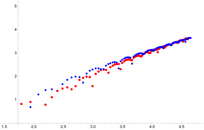
Figure 1: The vertical axis represents $\log\Bigl{(}\log|d^{(n=1)}_{M}[Q]|\Bigr{)}\,$ and the horizontal axis represents $\log Q\,$, with $Q$ ranging from $6$ to $80\,$. The vertical coordinates of the blue points come from evaluating the asymptotic formula  $\log(\frac{1}{3}X+\log|2\cos X|)\,$ where $X=\sqrt[4]{\frac{226}{5}}\pi\,\sqrt{3}{(Q/6)}^{3/4}$. The vertical positions of the red points come from taking $\log(\log|\cdot|)$ of the coefficients in (313).

Notice that the giant graviton index at fixed $n$ grows faster than the total giant graviton index in the limit (308). How are these cancellations explained in the present approach? Let us define the variable $\delta n$

$$\delta n:=\frac{N}{\Lambda^{4}}\,n\,,$$ (316)

which ranges over a continuum domain in the limit as $\Lambda\to\infty$. Then we can trade the sum over $n$ by an integral over a finite segment of length $\widetilde{q}^{\prime}=O(1)$ as $\Lambda\to\infty$ that can be evaluated by saddle-point approximation (as it is Gaussian):

$$\begin{split}\,\sum_{n\,=\,0}^{\lfloor\widetilde{Q}^{\prime}/N\rfloor}\,e^{\Bigl{(}\frac{4\pi^{4}}{3}\frac{{\overline{B}_{4}}\left[\frac{1}{2}+\frac{{\rm i}\omega_{1}}{2\pi}\right]-{\overline{B}_{4}}\left[\frac{{\rm i}\omega_{1}}{2\pi}\right]-\frac{1}{16}}{\Delta_{1}\Delta_{2}\Delta_{3}\epsilon^{3}}\Bigr{)}\,n^{2}}&\,\underset{\Lambda\to\infty}{\sim_{\text{exp}}}\,\int^{\widetilde{q}^{\prime}}_{0}d[\delta n]e^{\Bigl{(}\frac{4\pi^{4}}{3}\frac{{\overline{B}_{4}}\left[\frac{1}{2}+\frac{{\rm i}\omega_{1}}{2\pi}\right]-{\overline{B}_{4}}\left[\frac{{\rm i}\omega_{1}}{2\pi}\right]-\frac{1}{16}}{\Delta_{1}\Delta_{2}\Delta_{3}\epsilon^{3}}\Bigr{)}\,\frac{\Lambda^{8}}{N^{2}}\,\delta n^{2}}\\ &\underset{\Lambda\to\infty}{\sim_{\text{exp}}}\,1\,.\end{split}$$ (317)

This mechanism explains how these contributions do not compete with the ones coming from the singularity locus at $\zeta_{i}=1$ (encoded in (301)) in determinining the total microcanonical giant graviton index (287) at large charges.

References

• (1) J. Kinney, J. M. Maldacena, S. Minwalla, and S. Raju, An Index for 4 dimensional super conformal theories, Commun. Math. Phys. 275 (2007) 209–254, [hep-th/0510251].
• (2) C. Romelsberger, Counting chiral primaries in N = 1, d=4 superconformal field theories, Nucl. Phys. B747 (2006) 329–353, [hep-th/0510060].
• (3) Y. Imamura, Finite-N superconformal index via the AdS/CFT correspondence, PTEP 2021 (2021), no. 12 123B05, [arXiv:2108.12090].
• (4) R. Arai and Y. Imamura, Finite $N$ Corrections to the Superconformal Index of S-fold Theories, PTEP 2019 (2019), no. 8 083B04, [arXiv:1904.09776].
• (5) D. Gaiotto and J. H. Lee, The Giant Graviton Expansion, arXiv:2109.02545.
• (6) J. H. Lee, Exact stringy microstates from gauge theories, JHEP 11 (2022) 137, [arXiv:2204.09286].
• (7) S. Murthy, The growth of the $\frac{1}{16}$-BPS index in 4d $\mathcal{N}=4$ SYM, arXiv:2005.10843.
• (8) P. Agarwal, S. Choi, J. Kim, S. Kim, and J. Nahmgoong, AdS black holes and finite N indices, arXiv:2005.11240.
• (9) A. Cabo-Bizet, D. Cassani, D. Martelli, and S. Murthy, Microscopic origin of the Bekenstein-Hawking entropy of supersymmetric AdS5 black holes, JHEP 10 (2019) 062, [arXiv:1810.11442].
• (10) S. Choi, J. Kim, S. Kim, and J. Nahmgoong, Large AdS black holes from QFT, arXiv:1810.12067.
• (11) F. Benini and E. Milan, Black Holes in 4D $\mathcal{N}$=4 Super-Yang-Mills Field Theory, Phys. Rev. X 10 (2020), no. 2 021037, [arXiv:1812.09613].
• (12) S. Murthy, Unitary matrix models, free fermions, and the giant graviton expansion, Pure Appl. Math. Quart. 19 (2023), no. 1 299–340, [arXiv:2202.06897].
• (13) J. T. Liu and N. J. Rajappa, Finite N indices and the giant graviton expansion, JHEP 04 (2023) 078, [arXiv:2212.05408].
• (14) D. S. Eniceicu, Comments on the Giant-Graviton Expansion of the Superconformal Index, arXiv:2302.04887.
• (15) D. Berenstein and S. Wang, BPS coherent states and localization, JHEP 08 (2022) 164, [arXiv:2203.15820].
• (16) H. Lin, Coherent state operators, giant gravitons, and gauge-gravity correspondence, Annals Phys. 451 (2023) 169248, [arXiv:2212.14002].
• (17) M. Beccaria and A. Cabo-Bizet, On the brane expansion of the Schur index, JHEP 08 (2023) 073, [arXiv:2305.17730].
• (18) M. Honda, Quantum Black Hole Entropy from 4d Supersymmetric Cardy formula, Phys. Rev. D100 (2019), no. 2 026008, [arXiv:1901.08091].
• (19) A. Arabi Ardehali, Cardy-like asymptotics of the 4d $\mathcal{N}=4$ index and AdS5 blackholes, JHEP 06 (2019) 134, [arXiv:1902.06619].
• (20) J. Kim, S. Kim, and J. Song, A 4d $\mathcal{N}$ = 1 Cardy Formula, JHEP 01 (2021) 025, [arXiv:1904.03455].
• (21) A. Cabo-Bizet, D. Cassani, D. Martelli, and S. Murthy, The asymptotic growth of states of the 4d $\mathcal{N}=1$ superconformal index, JHEP 08 (2019) 120, [arXiv:1904.05865].
• (22) D. Cassani and Z. Komargodski, EFT and the SUSY Index on the 2nd Sheet, SciPost Phys. 11 (2021) 004, [arXiv:2104.01464].
• (23) S. Choi, S. Kim, E. Lee, and J. Lee, From giant gravitons to black holes, arXiv:2207.05172.
• (24) J. B. Gutowski and H. S. Reall, Supersymmetric AdS5 black holes, JHEP 02 (2004) 006, [hep-th/0401042].
• (25) J. B. Gutowski and H. S. Reall, General supersymmetric AdS(5) black holes, JHEP 04 (2004) 048, [hep-th/0401129].
• (26) M. Cvetic, H. Lu, and C. Pope, Charged rotating black holes in five dimensional U(1)**3 gauged N=2 supergravity, Phys. Rev. D 70 (2004) 081502, [hep-th/0407058].
• (27) A. Cabo-Bizet, From multi-gravitons to Black holes: The role of complex saddles, arXiv:2012.04815.
• (28) A. Cabo-Bizet and S. Murthy, Supersymmetric phases of 4d $\mathcal{N}$ = 4 SYM at large $N$, JHEP 09 (2020) 184, [arXiv:1909.09597].
• (29) A. Cabo-Bizet, D. Cassani, D. Martelli, and S. Murthy, The large-$N$ limit of the 4d $\mathcal{N}$ = 1 superconformal index, JHEP 11 (2020) 150, [arXiv:2005.10654].
• (30) O. Aharony, F. Benini, O. Mamroud, and E. Milan, A gravity interpretation for the Bethe Ansatz expansion of the $\mathcal{N}=4$ SYM index, Phys. Rev. D 104 (2021) 086026, [arXiv:2104.13932].
• (31) O. Mamroud, The SUSY Index Beyond the Cardy Limit, arXiv:2212.11925.
• (32) Y. Chen, M. Heydeman, Y. Wang, and M. Zhang, Probing Supersymmetric Black Holes with Surface Defects, arXiv:2306.05463.
• (33) D. E. Berenstein, J. M. Maldacena, and H. S. Nastase, Strings in flat space and pp waves from N=4 superYang-Mills, JHEP 04 (2002) 013, [hep-th/0202021].
• (34) L. F. Alday and J. M. Maldacena, Comments on operators with large spin, JHEP 11 (2007) 019, [arXiv:0708.0672].
• (35) B. Basso and G. P. Korchemsky, Anomalous dimensions of high-spin operators beyond the leading order, Nucl. Phys. B 775 (2007) 1–30, [hep-th/0612247].
• (36) Z. Komargodski and A. Zhiboedov, Convexity and Liberation at Large Spin, JHEP 11 (2013) 140, [arXiv:1212.4103].
• (37) A. L. Fitzpatrick, J. Kaplan, D. Poland, and D. Simmons-Duffin, The Analytic Bootstrap and AdS Superhorizon Locality, JHEP 12 (2013) 004, [arXiv:1212.3616].
• (38) L. Alvarez-Gaume, D. Orlando, and S. Reffert, Selected topics in the large quantum number expansion, Physics Reports 933 (oct, 2021) 1–66.
• (39) A. González Lezcano, J. Hong, J. T. Liu, and L. A. Pando Zayas, Sub-leading Structures in Superconformal Indices: Subdominant Saddles and Logarithmic Contributions, arXiv:2007.12604.
• (40) K. Goldstein, V. Jejjala, Y. Lei, S. van Leuven, and W. Li, Residues, modularity, and the Cardy limit of the 4d $\mathcal{N}=4$ superconformal index, arXiv:2011.06605.
• (41) A. Amariti, M. Fazzi, and A. Segati, The SCI of $\mathcal{N}$ = 4 USp(2Nc) and SO(Nc) SYM as a matrix integral, JHEP 06 (2021) 132, [arXiv:2012.15208].
• (42) A. Amariti, M. Fazzi, and A. Segati, Expanding on the Cardy-like limit of the SCI of 4d $\mathcal{N}$ = 1 ABCD SCFTs, JHEP 07 (2021) 141, [arXiv:2103.15853].
• (43) A. Arabi Ardehali and S. Murthy, The 4d superconformal index near roots of unity and 3d Chern-Simons theory, arXiv:2104.02051.
• (44) V. Jejjala, Y. Lei, S. van Leuven, and W. Li, $SL(3,\mathbb{Z})$ Modularity and New Cardy Limits of the $\mathcal{N}=4$ Superconformal Index, arXiv:2104.07030.
• (45) A. A. Ardehali and J. Hong, Decomposition of BPS Moduli Spaces and Asymptotics of Supersymmetric Partition Functions, arXiv:2110.01538.
• (46) A. Cabo-Bizet, On the 4d superconformal index near roots of unity: bulk and localized contributions, JHEP 02 (2023) 134, [arXiv:2111.14941].
• (47) A. Cabo-Bizet, Quantum phases of 4d SU(N) $\mathcal{N}$ = 4 SYM, JHEP 10 (2022) 052, [arXiv:2111.14942].
• (48) V. Jejjala, Y. Lei, S. van Leuven, and W. Li, Modular factorization of superconformal indices, arXiv:2210.17551.
• (49) A. Amariti and A. Zanetti, S-duality in the Cardy-like limit of the superconformal index, arXiv:2307.08391.
• (50) S. Choi, C. Hwang, and S. Kim, Quantum vortices, M2-branes and black holes, arXiv:1908.02470.
• (51) J. Nian and L. A. Pando Zayas, Microscopic entropy of rotating electrically charged AdS4 black holes from field theory localization, JHEP 03 (2020) 081, [arXiv:1909.07943].
• (52) A. González Lezcano, M. Jerdee, and L. A. Pando Zayas, Cardy expansion of 3d superconformal indices and corrections to the dual black hole entropy, JHEP 01 (2023) 044, [arXiv:2210.12065].
• (53) P. Benetti Genolini, A. Cabo-Bizet, and S. Murthy, Supersymmetric phases of AdS4/CFT3, arXiv:2301.00763.
• (54) A. Amariti, J. Nian, L. A. Pando Zayas, and A. Segati, Universal Cardy-Like Behavior of 3D A-Twisted Partition Functions, arXiv:2306.05462.
• (55) N. Bobev, V. Dimitrov, V. Reys, and A. Vekemans, Higher derivative corrections and AdS5 black holes, Phys. Rev. D 106 (2022), no. 12 L121903, [arXiv:2207.10671].
• (56) D. Cassani, A. Ruipérez, and E. Turetta, Corrections to AdS5 black hole thermodynamics from higher-derivative supergravity, JHEP 11 (2022) 059, [arXiv:2208.01007].
• (57) D. Cassani, A. Ruipérez, and E. Turetta, Boundary terms and conserved charges in higher-derivative gauged supergravity, arXiv:2304.06101.
• (58) M. Berkooz, D. Reichmann, and J. Simon, A Fermi Surface Model for Large Supersymmetric AdS(5) Black Holes, JHEP 01 (2007) 048, [hep-th/0604023].
• (59) M. Berkooz and D. Reichmann, Weakly Renormalized Near 1/16 SUSY Fermi Liquid Operators in N=4 SYM, JHEP 10 (2008) 084, [arXiv:0807.0559].
• (60) C.-M. Chang, L. Feng, Y.-H. Lin, and Y.-X. Tao, Decoding stringy near-supersymmetric black holes, arXiv:2306.04673.
• (61) K. Budzik, H. Murali, and P. Vieira, Following Black Hole States, arXiv:2306.04693.
• (62) J. a. Caetano, S. Komatsu, and Y. Wang, Large Charge ’t Hooft Limit of $\mathcal{N}=4$ Super-Yang-Mills, arXiv:2306.00929.
• (63) J. Boruch, M. T. Heydeman, L. V. Iliesiu, and G. J. Turiaci, BPS and near-BPS black holes in $AdS_{5}$ and their spectrum in $\mathcal{N}=4$ SYM, arXiv:2203.01331.
• (64) G. J. Turiaci and E. Witten, $\mathcal{N}=2$ JT Supergravity and Matrix Models, arXiv:2305.19438.
• (65) C.-M. Chang and X. Yin, 1/16 BPS states in $\mathcal{N}=$ 4 super-Yang-Mills theory, Phys. Rev. D88 (2013), no. 10 106005, [arXiv:1305.6314].
• (66) F. A. Dolan and H. Osborn, Applications of the Superconformal Index for Protected Operators and q-Hypergeometric Identities to N=1 Dual Theories, Nucl. Phys. B 818 (2009) 137–178, [arXiv:0801.4947].
• (67) F. Benini and E. Milan, A Bethe Ansatz type formula for the superconformal index, Commun. Math. Phys. 376 (2020), no. 2 1413–1440, [arXiv:1811.04107].
• (68) A. Narukawa, The modular properties and the integral representations of the multiple elliptic gamma functions, math/0306164.
• (69) G. Felder and A. Varchenko Advances in Mathematics 156 (2000), no. 1 44–76, [9907061].