Measurement of branching-fraction ratios and $C\!P$ asymmetries in $B^{\pm}\rightarrow D_{C\!P\pm}K^{\pm}$ decays at Belle and Belle II

Abstract

We report results from a study of $B^{\pm}\rightarrow DK^{\pm}$ decays followed by $D$ decaying to $C\!P$ eigenstates, where $D$ indicates a $D^{0}$ or $\kern 1.99997pt\overline{\kern-1.99997ptD}{}^{0}$ meson. These decays are sensitive to the Cabibbo-Kobayashi-Maskawa unitarity-triangle angle $\phi_{3}$. The results are based on a combined analysis of the final data set of $772\times 10^{6}~{}B\bar{B}$ pairs collected by the Belle experiment and a data set of $198\times 10^{6}~{}B\bar{B}$ pairs collected by the Belle II experiment, both in electron-positron collisions at the $\Upsilon(4S)$ resonance. We measure the $C\!P$ asymmetries to be $\mathcal{A}_{C\!P+}=~{}(+12.5\pm 5.8\pm 1.4)\%$ and $\mathcal{A}_{C\!P-}=~{}(-16.7\pm 5.7\pm 0.6)\%$, and the ratios of branching fractions to be $\mathcal{R}_{C\!P+}=~{}1.164\pm 0.081\pm 0.036$ and $\mathcal{R}_{C\!P-}=~{}1.151\pm 0.074\pm 0.019$. The first contribution to the uncertainties is statistical, and the second is systematic. The asymmetries $\mathcal{A}_{C\!P+}$ and $\mathcal{A}_{C\!P-}$ have similar magnitudes and opposite signs; their difference corresponds to 3.5 standard deviations. From these values we calculate 68.3% confidence intervals of ($8.5^{\circ}<\phi_{3}<16.5^{\circ}$) or ($84.5^{\circ}<\phi_{3}<95.5^{\circ}$) or ($163.3^{\circ}<\phi_{3}<171.5^{\circ}$) and $0.321<r_{B}<0.465$.

1 Introduction

The Cabibbo-Kobayashi-Maskawa (CKM) matrix parameterizes quark mixing in the standard model Cabibbo ; KM . The angle $\phi_{3}$, also called $\gamma$, is the phase of a product of its elements $-V_{\it ud}V^{*}_{\it ub}/V_{\it cd}^{*}V_{\it cb}$. Theoretical relationships connecting the angle $\phi_{3}$ with rates and $C\!P$ asymmetries of the decays $B^{\pm}\rightarrow DK^{\pm}$, where $D$ indicates a $D^{0}$ or $\kern 1.99997pt\overline{\kern-1.99997ptD}{}^{0}$ meson, are reliable and can be used for precise direct measurements of $\phi_{3}$. Any inconsistency between direct measurements of $\phi_{3}$ and the value inferred from global CKM fits performed without this information would show that the CKM mechanism is not a complete description of $C\!P$ violation and reveal effects of physics beyond the standard model. Gronau, London, and Wyler (GLW) proposed a method to extract $\phi_{3}$ using decays in which the neutral $D$, $D_{C\!P\pm}$, is reconstructed as a $C\!P$ eigenstate GLW1 ; GLW2 . We use this method to determine $\phi_{3}$ using combined data sets of the Belle and Belle II experiments.

We measure $C\!P$ asymmetries,

$$\mathcal{A}_{C\!P\pm}\equiv\frac{\mathcal{B}(B^{-}\rightarrow D_{C\!P\pm}K^{-})-\mathcal{B}(B^{+}\rightarrow D_{C\!P\pm}K^{+})}{\mathcal{B}(B^{-}\rightarrow D_{C\!P\pm}K^{-})+\mathcal{B}(B^{+}\rightarrow D_{C\!P\pm}K^{+})},$$ (1)

and the ratio of branching fractions for decays in which the $D$ is reconstructed as a $C\!P$ eigenstate and decays in which the $D$ is reconstructed in a flavor-specific state:

$$\mathcal{R}_{C\!P\pm}\equiv\frac{\mathcal{B}(B^{-}\rightarrow D_{C\!P\pm}K^{-})+\mathcal{B}(B^{+}\rightarrow D_{C\!P\pm}K^{+})}{(\mathcal{B}(B^{-}\rightarrow D_{\rm flav}K^{-})+\mathcal{B}(B^{+}\rightarrow\kern 1.99997pt\overline{\kern-1.99997ptD}{}_{\rm flav}K^{+}))/2}.$$ (2)

This ratio can be expressed as

$$\mathcal{R}_{C\!P\pm}\approx\frac{R_{C\!P\pm}}{R_{\text{flav}}},$$ (3)

where

$$R_{C\!P\pm}\equiv\frac{\mathcal{B}(B^{-}\rightarrow D_{C\!P\pm}K^{-})+\mathcal{B}(B^{+}\rightarrow D_{C\!P\pm}K^{+})}{\mathcal{B}(B^{-}\rightarrow D_{C\!P\pm}\pi^{-})+\mathcal{B}(B^{+}\rightarrow D_{C\!P\pm}\pi^{+})},$$ (4)

and

$$R_{\rm flav}\equiv\frac{\mathcal{B}(B^{-}\rightarrow D_{\rm flav}K^{-})+\mathcal{B}(B^{+}\rightarrow\kern 1.99997pt\overline{\kern-1.99997ptD}{}_{\rm flav}K^{+})}{\mathcal{B}(B^{-}\rightarrow D_{\rm flav}\pi^{-})+\mathcal{B}(B^{+}\rightarrow\kern 1.99997pt\overline{\kern-1.99997ptD}{}_{\rm flav}\pi^{+})}.$$ (5)

In these ratios of branching fractions, most systematic uncertainties, such as those from reconstruction efficiencies and the known $D$ branching fractions, cancel. The approximation in equation 3 is an equality if $C\!P$ is conserved in the $B^{\pm}\rightarrow D\pi^{\pm}$ decay. Neglecting the small effects of $D$ mixing and $C\!P$ violation in the $D^{0}$ decay Rama:2013voa , we relate $\mathcal{R}_{C\!P\pm}$ and $\mathcal{A}_{C\!P\pm}$ to $\phi_{3}$, the ratio $r_{B}$ of the magnitudes of the suppressed to favored $B^{\pm}\rightarrow DK^{\pm}$ amplitudes, and the relative interaction phase $\delta_{B}$ between them PDG :

$$\mathcal{R}_{C\!P\pm} =1+r_{B}^{2}\pm 2r_{B}\cos\delta_{B}\cos\phi_{3},$$ (6)

$$\mathcal{A}_{C\!P\pm} =\pm 2r_{B}\sin\delta_{B}\sin\phi_{3}\,/\,\mathcal{R}_{C\!P\pm}.$$ (7)

The current precision on $\phi_{3}$ is about $3.5^{\circ}$ PDG ; HFLAV , dominated by recent measurements from the LHCb experiment gammaLHCb . The Belle experiment reported a $\phi_{3}$-related measurement using the ADS method ADS1 ; ADS2 for $B^{\pm}\rightarrow DK^{\pm}$ decays with $D\rightarrow K^{\pm}\pi^{\mp}$ using its full data set ADS_Belle . A measurement using the BPGGSZ method GGSZ1 ; GGSZ2 for $B^{\pm}\rightarrow Dh^{\pm}$ decays with $D\rightarrow K^{0}_{\rm\scriptscriptstyle S}h^{\pm}h^{\mp}$, where $h$ is a pion or kaon, using the full Belle data set and $128\text{\,}\mathrm{f}\mathrm{b}^{-1}$ of data from Belle II was reported recently GGSZB2 . However, Belle reported results using the GLW $B^{\pm}\rightarrow D^{(*)}K^{\pm}$ decays based only a fraction of its data GLW_Belle . Here we report results based on the full Belle data set and also a fraction of the available data from Belle II. These results supersede those of Ref. GLW_Belle .

2 Data samples and detectors

We analyze samples containing $772\text{\times}{10}^{6}$ and $198\text{\times}{10}^{6}$ $B\kern 1.79993pt\overline{\kern-1.79993ptB}{}$ pairs collected in electron-positron collisions at the $\Upsilon(4S)$ resonance with the Belle and Belle II detectors. The integrated luminosities of the corresponding data sets are $711\text{\,}\mathrm{f}\mathrm{b}^{-1}$ and $189\text{\,}\mathrm{f}\mathrm{b}^{-1}$ for Belle and Belle II. Belle operated at the KEKB asymmetric-energy collider with electron- and positron-beam energies of $8\text{\,}\mathrm{G}\mathrm{e}\mathrm{V}$ and $3.5\text{\,}\mathrm{G}\mathrm{e}\mathrm{V}$ KEKB ; KEKB_achievement , respectively. Belle II operates at its successor, SuperKEKB, designed to deliver thirty times higher instantaneous luminosity than KEKB, with electron- and positron-beam energies of $7\text{\,}\mathrm{G}\mathrm{e}\mathrm{V}$ and $4\text{\,}\mathrm{G}\mathrm{e}\mathrm{V}$ superKEKB , respectively.

The Belle detector Belle_detector ; Belle_detector_achivement was a large-solid-angle magnetic spectrometer that consisted of a silicon vertex detector, a 50-layer central drift chamber, an array of aerogel threshold Cherenkov counters, a barrel-like arrangement of time-of-flight scintillation counters, and an electromagnetic calorimeter, all located within a superconducting solenoid coil that provided a uniform $1.5\text{\,}\mathrm{T}$ magnetic field collinear with the beams. An iron flux-return yoke located outside the coil was instrumented to detect $K^{0}_{\rm\scriptscriptstyle L}$ and muons.

The Belle II detector Belle2det is an upgrade with several new subdetectors designed to handle the significantly larger beam-related backgrounds of the new collider. It consists of a silicon vertex detector comprising two inner layers of pixel detectors and four outer layers of double-sided silicon strip detectors, a 56-layer central drift chamber, a time-of-propagation detector in the central detector volume and an aerogel ring-imaging Cherenkov detector in the forward region (with respect to the electron-beam’s direction) for charged particle identification (PID), and an electromagnetic calorimeter, all located inside the same solenoid as used for Belle. A flux return outside the solenoid is instrumented with resistive-plate chambers, plastic scintillator modules, and an upgraded read-out system to detect muons, $K^{0}_{\rm\scriptscriptstyle L}$ mesons, and neutrons.

We use simulated data to optimize selection criteria, determine detection efficiencies, train multivariate discriminants, identify sources of background, and obtain our fit models. The EvtGen software package is used to simulate the $e^{+}e^{-}\rightarrow\Upsilon(4S)\rightarrow B\kern 1.79993pt\overline{\kern-1.79993ptB}{}$ process and our signal decays EVTGEN . The KKMC KKMC and Pythia PYTHIA generators are used to simulate the $e^{+}e^{-}\rightarrow q\overline{}q$ continuum, where $q$ indicates a $u,d,s$ or $c$ quark. For Belle, the Geant3 package GSIM was used to model the detector response, whereas for Belle II the Geant4 package GEANT4 is used. To account for final-state radiation, the Photos package PHOTOS is used.

3 Reconstruction and candidate selection

We use the Belle II analysis software framework to reconstruct both Belle and Belle II data BASF2 ; basf2-zenodo ; B2BII . Owing to the different performance of the detectors, separate sets of selection criteria are used for each data set.

Online data-selection criteria are based on requirements of a minimum number of charged particles and observed energy in an event. They are fully efficient for signal and strongly suppress low-multiplicity events. In the offline analysis, reconstructed charged-particle trajectories (tracks) are required to have distances from the $e^{+}e^{-}$ interaction point (IP) smaller than $0.2\text{\,}\mathrm{c}\mathrm{m}$ in the plane transverse to the beams, and smaller than $1.0\text{\,}\mathrm{c}\mathrm{m}$ along the beam direction. Charged kaon and pion candidates are identified based on information from PID detectors and the specific ionisation measured in the drift chamber. We use the ratio $\mathcal{L}(K/\pi)\equiv{\mathcal{L}(K)}/{[\mathcal{L}(K)+\mathcal{L}(\pi)]}$ to identify the type of charged particles, where $\mathcal{L}(h)$ is the likelihood for a kaon or pion to produce the signals observed in the detectors. Charged particles with $\mathcal{L}(K/\pi)>0.6$ are identified as kaons, and those with $\mathcal{L}(K/\pi)<0.6$ as pions. To mitigate pion misidentification in the Belle II data, we remove tracks with a polar angle $\theta>120^{\circ}$, since no PID detector covers this region b2charm_conf . No such veto is necessary for Belle data because the larger KEKB boost results in essentially all tracks being within the acceptance of the PID detectors.

We reconstruct $K^{0}_{\rm\scriptscriptstyle S}$ candidates in their $\pi^{+}\pi^{-}$ final state by forming each from a pair of oppositely charged particles (assuming they are pions) with a common vertex and mass in the range $[486,509]$ $\mathrm{M}\mathrm{e}\mathrm{V}$/$c^{2}$ for Belle data and $[491,504]$ $\mathrm{M}\mathrm{e}\mathrm{V}$/$c^{2}$ for Belle II data. These ranges correspond to $3\sigma$ in resolution in either direction from the known $K^{0}$ mass. To improve the purity of the $K^{0}_{\rm\scriptscriptstyle S}$ sample, we reject combinatorial background using neural networks for Belle data and boosted decision trees for Belle II data nakano_thesis ; nakano_prd ; GGSZB2 . Five input variables are common to the Belle and Belle II discriminators: the angle between the $K^{0}_{\rm\scriptscriptstyle S}$ momentum and the direction from the IP to the $K^{0}_{\rm\scriptscriptstyle S}$ decay vertex; the distance-of-closest-approach to the IP of the pion tracks; the flight distance of the $K^{0}_{\rm\scriptscriptstyle S}$ in the plane transverse to the beams; and the difference between the measured and known $K^{0}_{\rm\scriptscriptstyle S}$ masses divided by the uncertainty of the measured mass. The Belle discriminator uses seven additional variables, including the $K^{0}_{\rm\scriptscriptstyle S}$ momentum and the shortest distance between the two track helices projected along the beam direction nakano_thesis ; nakano_prd . Each $K^{0}_{\rm\scriptscriptstyle S}$ momentum is recalculated from a fit of the pion momenta that constrains them to a common origin.

We reconstruct $\pi^{0}$ candidates via their decays to two photons. In Belle data, each photon is required to have an energy above $50\text{\,}\mathrm{M}\mathrm{e}\mathrm{V}$; in Belle II data, each photon is required to have an energy above $80\text{\,}\mathrm{M}\mathrm{e}\mathrm{V}$ if detected in the forward endcap, $30\text{\,}\mathrm{M}\mathrm{e}\mathrm{V}$ if detected in the barrel, and $60\text{\,}\mathrm{M}\mathrm{e}\mathrm{V}$ if in the backward endcap. Each photon must also be unassociated with any track and have an energy-deposition distribution in the calorimeter consistent with an electromagnetic shower. Each $\pi^{0}$ candidate must have a mass in the range $[120,145]$ $\mathrm{M}\mathrm{e}\mathrm{V}$/$c^{2}$, corresponding to $2.5\sigma$ in resolution on either side of the known $\pi^{0}$ mass, and momentum above $0.6\text{\,}\mathrm{G}\mathrm{e}\mathrm{V}$/$c$. Each $\pi^{0}$ momentum is recalculated from a fit of the photon momenta that constrains them to a common origin and the diphoton mass to the known mass of the $\pi^{0}$.

A $D$ candidate is formed from combinations of $K^{-}$ and $\pi^{+}$, $K^{+}$ and $K^{-}$, and $K^{0}_{\rm\scriptscriptstyle S}$ and $\pi^{0}$ candidates. The mass of each $D$ candidate is required to be consistent with the known $D$ mass PDG within $[-20,+20]$ $\mathrm{M}\mathrm{e}\mathrm{V}$/$c^{2}$ in Belle data and $[-12,+12]$ $\mathrm{M}\mathrm{e}\mathrm{V}$/$c^{2}$ in Belle II data for $D\rightarrow K^{\pm}h^{\mp}$ decays; and within $[-64,+47]$ $\mathrm{M}\mathrm{e}\mathrm{V}$/$c^{2}$ in Belle data and $[-53,+36]$ $\mathrm{M}\mathrm{e}\mathrm{V}$/$c^{2}$ in Belle II data for the $D\rightarrow K^{0}_{\rm\scriptscriptstyle S}\pi^{0}$ decays. These ranges are approximately $3\sigma$ in resolution on either side of the known mass. Each $D$ momentum is recalculated from a fit of the momenta of its decay products that constrains them to a common origin and their invariant mass to the known mass of the $D$ meson.

A $B$ candidate is formed from a $D$ candidate and an $h^{\pm}$ candidate. To select signal candidates, we use the beam-energy-constrained mass,

$$M_{\text{bc}}\equiv c^{-2}\sqrt{E_{\text{beam}}^{*2}-|\vec{p}_{B}c|^{2}},$$ (8)

and the energy difference, $\Delta E\equiv E_{B}-E_{\text{beam}}^{*}$, calculated from the $B$ energy $E_{B}$, momentum $\vec{p}_{B}$, and beam energy $E_{\text{beam}}^{*}$, all in the center-of-mass (c.m.) frame. We require $M_{\text{bc}}$ to be in the range $[5.27,5.29]$ $\mathrm{G}\mathrm{e}\mathrm{V}$/$c^{2}$, which is $\pm 3\sigma$ in resolution around the known $B$ mass PDG . We require $\Delta E$ to be in the range $[-0.13,0.15]$ $\mathrm{G}\mathrm{e}\mathrm{V}$ to suppress partially reconstructed $B^{\pm}\rightarrow D^{*}h^{\pm}$ decays, which have negative $\Delta E$.

Most remaining backgrounds arise from continuum events, in which final-state particles are highly boosted into two jets that are approximately back-to-back in the c.m. frame. Since $B\kern 1.79993pt\overline{\kern-1.79993ptB}{}$ pairs are produced slightly above kinematic threshold, their final-state particles are isotropically distributed in the c.m. frame. We use boosted decision trees (BDTs) to suppress candidates from continuum events. We train them on equal numbers of simulated signal and continuum events using variables that are uncorrelated with $\Delta E$. Those variables are well simulated, as verified by inspection of the flavor-specific channel. The variables used are modified Fox-Wolfram moments KSFW1 ; KSFW2 ; the cosine of the polar angle of the $B$ momentum in the c.m. frame; the absolute value of the cosine of the angle between the thrust axis of the $B$ and the thrust axis of the rest of the charged particles and photons in the event (ROE); the longitudinal distance between the $B$ vertex and the ROE vertex; and the output of a $B$-flavor-tagging algorithm flavor_tag1 ; flavor_tag2 . The thrust axis of a group of particles is the direction that maximizes the sum of the projections of the particle momenta onto it. The BDT classifier output, $\mathcal{C}$, is in the range $[0,1]$, peaking at zero for continuum background and at one for signal. We require $\mathcal{C}>0.15$, which retains 95% of signal in Belle data and 97% in Belle II data, while rejecting 60% and 63% of background, respectively.

To suppress $D$ decays from $D^{*}\rightarrow D\pi$ arising from $e^{+}e^{-}\rightarrow c\overline{c}\rightarrow D^{*}D^{(*)}X$ processes, we use the observed difference between the mass of the $D$ candidate and the mass of the $D^{*}$ candidates reconstructed by associating to the $D$ any $\pi^{\pm}$ or $\pi^{0}$ in the ROE. We require that the differences all be outside $\pm 3\sigma$ in resolution from the known $D^{*}$-$D$ mass difference PDG ; the excluded ranges are [143.4, 147.5] $\mathrm{M}\mathrm{e}\mathrm{V}$/$c^{2}$ and [143.8, 147.0] $\mathrm{M}\mathrm{e}\mathrm{V}$/$c^{2}$ in Belle and Belle II data for $D^{*\pm}$, respectively, and [140.0, 145.0] $\mathrm{M}\mathrm{e}\mathrm{V}$/$c^{2}$ in both experiments for $D^{*0}$. This retains 97% of signal candidates and rejects 13% of background candidates in Belle data and 18% in Belle II data. For $B^{\pm}\rightarrow D(\rightarrow K^{\pm}\pi^{\mp})\pi^{\pm}$, we require that the dipion mass not be in the range $[3.08,3.14]$ $\mathrm{G}\mathrm{e}\mathrm{V}$/$c^{2}$ to veto candidates reconstructed from $B^{\pm}\rightarrow{J\mskip-3.0mu/\mskip-2.0mu\psi\mskip 2.0mu}(\rightarrow\ell^{+}\ell^{-})K^{\pm}$ decays in which both leptons are misidentified. The $\Delta E$ distribution of such events peaks in the signal region.

In events with multiple $B$ candidates, 2% of events for the $C\!P$-even mode and 7% for the $C\!P$-odd mode, we retain the candidate with the smallest $\chi^{2}$ calculated from the reconstructed $D$ mass, $M_{\text{bc}}$ and their resolutions; for decays with $D_{C\!P-}$, the reconstructed $\pi^{0}$ mass and its resolution are also used in the $\chi^{2}$ calculation. This selects the correct signal candidate in 70%–80% of such events in simulation.

4 Fits to data

The final event sample consists of signal, cross-feed background that comes from mis-identifying the $h^{\pm}$ of a signal event, other $B\kern 1.79993pt\overline{\kern-1.79993ptB}{}$ background sources, and continuum background. To determine the numbers of signal candidates, we fit to the distributions of $\Delta E$ and $\mathcal{C}$, the variables that best discriminate between signal and the remaining background. To make $\mathcal{C}$ easier to model, we transform it to a new variable $\mathcal{C}^{\prime}$, such that signal is distributed uniformly in $[0,1]$ and background is exponentially distributed mu_trans . We perform an unbinned extended maximum-likelihood fit to candidates with $\Delta E\in[-0.13,0.14]~{}$\mathrm{G}\mathrm{e}\mathrm{V}$$ and $\mathcal{C}^{\prime}$ in its full range.

Simulation shows that $\Delta E$–$\mathcal{C}^{\prime}$ correlations in the distributions of candidates from all sample components are negligible, and thus we factorize the two-dimensional probability density function (PDF) for each component in the fit. For each decay mode, we divide the data into 12 subsets defined by the product of the two possible electric charges of the $B$, the three possible $D$ final states (two $C\!P$-specific and one flavor-specific), and whether $h^{\pm}$ is identified as a kaon or pion. The fit models are mostly common in all decay modes and data subsets, but the shape parameters are different in each.

For signal, the $\Delta E$ PDF is the sum of two Gaussian functions and an asymmetric Gaussian function, with all parameters fixed from simulated data except for the common mean of all three $D$ decay modes and a common multiplier for all signal widths. These parameters are determined by the fit and account for differences in resolution between the experimental and simulated data. The $\mathcal{C}^{\prime}$ PDF is a straight line with its slope fixed to the value fitted in the simulated data, except for the PDF used for the Belle $D\pi$ data, in which the slope is a free parameter.

The cross-feed $\Delta E$ PDF is same to the signal one, but with its own set of parameters. When determining the fixed parameters of the cross-feed PDF for $D\pi$, the simulated data are corrected for momentum-dependent differences in particle misidentification rates between the experimental and simulated data. The $\mathcal{C}^{\prime}$ PDF is the sum of a straight line and an exponential function, with parameters fixed from the simulated samples.

For the $B\kern 1.79993pt\overline{\kern-1.79993ptB}{}$ background component, the $\Delta E$ PDF is the sum of an exponential function and a uniform distribution for the $C\!P$ modes, and the sum of an exponential function and a Novosibirsk function novo for the flavor-specific mode. The $\mathcal{C}^{\prime}$ PDF is a straight line whose slope is fixed from simulated data. A peaking background originates from events in which a $B$ decays directly to $Xh$ without the production of an intermediate charmed meson in the decay chain. This background is estimated from the $D$ mass sidebands in data, We find no peaking structure in the sideband of the $D_{C\!P-}$ mode, while for the $D_{C\!P+}$ mode we see a significant peaking structure and estimate its yield in the signal $\Delta E$ region to be $132\pm 17$ events in Belle data and $24\pm 4$ in Belle II data. These yields are estimated by linearly extrapolating the results obtained in eight $D$ mass sidebands in data, as discussed in Appendix B. In the final fit, the PDF shape of peaking background is fixed from a simulated sample.

For the continuum component, the $\Delta E$ PDF is a straight line and the $\mathcal{C}^{\prime}$ PDF is the sum of two exponential functions. The larger exponential component has its parameter fixed to the value fit from simulated data, and the other free to vary, which accounts for differences between the distributions in experimental and simulated data.

We perform a simultaneous fit to all decay modes in both the Belle and Belle II data, to determine the six charge asymmetries and three branching-fraction ratios. The yields of $B^{\pm}\rightarrow Dh^{\pm}$ with the $D$ decaying to the state $X$ and the charged hadron identified as $h^{\prime\pm}$, denoted as $Y_{h^{\prime}}(B^{\pm}\rightarrow D_{\!X}h^{\pm})$, are related to these physical observables via

$$Y_{\pi}(B^{\pm}\rightarrow D_{\!X}K^{\pm}) =\tfrac{1}{2}[1\mp\mathcal{A}(B\rightarrow D_{\!X}K)]\,N(B\rightarrow D_{\!X}\pi)\,R_{X}\,\delta\,(1-\varepsilon_{\pm}),$$ (9)

$$Y_{K}(B^{\pm}\rightarrow D_{\!X}K^{\pm}) =\tfrac{1}{2}[1\mp\mathcal{A}(B\rightarrow D_{\!X}K)]\,N(B\rightarrow D_{\!X}\pi)\,R_{X}\,\delta\,\varepsilon_{\pm},$$ (10)

$$Y_{\pi}(B^{\pm}\rightarrow D_{\!X}\pi^{\pm}) =\tfrac{1}{2}[1\mp\mathcal{A}(B\rightarrow D_{\!X}\pi)]\,N(B\rightarrow D_{\!X}\pi)\,(1-\kappa_{\pm}),$$ (11)

$$Y_{K}(B^{\pm}\rightarrow D_{\!X}\pi^{\pm}) =\tfrac{1}{2}[1\mp\mathcal{A}(B\rightarrow D_{\!X}\pi)]\,N(B\rightarrow D_{\!X}\pi)\,\kappa_{\pm},$$ (12)

where $\mathcal{A}$ is the charge asymmetry, $N$ is the total number of events regardless of how the charged hadron was identified and of its sign, $\varepsilon_{\pm}$ is the efficiency to identify a kaon with $\pm 1$ charge, and $\kappa_{\pm}$ is the rate for misidentifying a pion as a kaon with $\pm 1$ charge. The efficiency $\delta$ for reconstructing $B^{\pm}\rightarrow DK^{\pm}$ relative to that for $B^{\pm}\rightarrow D\pi^{\pm}$ is independent of the $D$ final state and equals 0.975 in Belle data and 1.000 in Belle II data. We measure PID efficiencies and misidentification rates using control samples. For Belle, we measure $\kappa_{+}=7.7\%$, $\kappa_{-}=8.2\%$, $\varepsilon_{+}=83.4\%$, and $\varepsilon_{-}=84.3\%$ belle_pid . For Belle II, we measure $\kappa_{+}=7.2\%$, $\kappa_{-}=8.7\%$, $\varepsilon_{+}=79.6\%$, and $\varepsilon_{-}=78.9\%$. Uncertainties on those values are typically 0.5%.

The signal yields $N$ are independent for the Belle and Belle II data. For each background component, separate yields are fitted for $B^{+}$ and $B^{-}$ to account for their possible charge asymmetries.

To check for fit biases, we perform the fit on five independent sets of simulated data. We also repeat the analysis on 1000 data sets simulated according to the fit model for seven different values of $\mathcal{A}_{C\!P\pm}$: 0, $\pm 0.1$, $\pm 0.2$, $\pm 0.3$. In all cases, the fit results are consistent with the input values.

5 Systematic uncertainties

We consider several sources of systematic uncertainties, which are summarized in Table 1. In general, for parameters fixed in the fits, we repeat the fits with the parameter varied by its uncertainty and take the resulting change in our results as the fit-model systematic uncertainty. We do this for the fixed PDF parameters, PID efficiencies and mis-identification rates, peaking background yields, and the efficiency ratio. We ignore correlations between those uncertainties and combine them by adding them in quadrature. We also assign systematic uncertainties (included in the "PDF parameters" item of Table 1) from the difference between correcting and not correcting for the momentum-dependent pion misidentification rates when modeling the cross-feed PDF for the $D\pi$ data, and having common and independent mode parameters for the $\Delta E$ PDF’s for $DK$ and $D\pi$. We use a common mean for the signal $\Delta E$ PDFs for all modes. The corresponding systematic uncertainty ("Signal-$\Delta E$ common mean" item of Table 1) is estimated from the variations resulting from assigning different mean values to the $\Delta E$ PDFs, i.e., $B\rightarrow D_{\!X}K$ and $B\rightarrow D_{\!X}\pi$ with the same or independent means, $B^{-}$ and $B^{+}$ with the same or independent means. For the slopes of the $\mathcal{C}^{\prime}$ PDF of the $B\kern 1.79993pt\overline{\kern-1.79993ptB}{}$ component, we calculate the systematic uncertainty from the maximum difference among fit results in which the slope is taken from simulation, as in the nominal fit, or taken from the signal $\mathcal{C}^{\prime}$ PDF’s slope in data, or determined by the fit itself.

Table 1: Systematic and statistical uncertainties.

	$\mathcal{R}_{C\!P+}$	$\mathcal{R}_{C\!P-}$	$\mathcal{A}_{C\!P+}$	$\mathcal{A}_{C\!P-}$
PDF parameters	$0.012$	$0.014$	$0.002$	$0.002$
PID parameters	$0.009$	$0.010$	$0.003$	$0.005$
Peaking background yields	$0.033$	$0.002$	$0.013$	—
Efficiency ratio	$0.001$	$0.001$	$<0.001$	$<0.001$
Signal-$\Delta E$ common mean	$0.005$	$0.006$	$<0.001$	$<0.001$
Total systematic uncertainty	$0.036$	$0.019$	$0.014$	$0.006$
Statistical uncertainty	$0.081$	$0.074$	$0.058$	$0.057$

6 Results

Figures 1, 3, and 5 show distributions and the fit results for candidates satisfying $|\Delta E|<0.05~{}\rm GeV$ and $0.65<\mathcal{C}^{\prime}<1.0$ for Belle data; figures 2, 4, and 6 show the corresponding plots for Belle II data. The fit results agree with the data; the small shifts seen for $B\rightarrow D_{\!X}\pi$ signal in $\Delta E$ are accounted for in the systematic uncertainty estimation. Table 2 summarizes the signal yields.

Table 2: Signal yields extracted from the simultaneous fit in data.

$D_{\!X}$ mode		$N(B\rightarrow D_{\!X}K)$	$N(B\rightarrow D_{\!X}\pi)$
$D\rightarrow K^{\pm}\pi^{\mp}$	Belle	$4238\pm 94$	$59481\pm 267$
	Belle II	$1084\pm 44$	$14229\pm 126$
$D\rightarrow K^{+}K^{-}$	Belle	$476\pm 36$	$5559\pm 85$
	Belle II	$107\pm 15$	$1336\pm 40$
$D\rightarrow K^{0}_{\rm\scriptscriptstyle S}\pi^{0}$	Belle	$541\pm 42$	$6484\pm 95$
	Belle II	$145\pm 16$	$1763\pm 46$

From the combined Belle and Belle II data, the ratios of branching-fraction ratios and $C\!P$ asymmetries of $B^{\pm}\rightarrow D_{C\!P}K^{\pm}$ are

$$\mathcal{R}_{C\!P+} =1.164\pm 0.081\pm 0.036,$$ (13)

$$\mathcal{R}_{C\!P-} =1.151\pm 0.074\pm 0.019,$$ (14)

$$\mathcal{A}_{C\!P+} =(+12.5\pm 5.8\pm 1.4)\%,$$ (15)

$$\mathcal{A}_{C\!P-} =(-16.7\pm 5.7\pm 0.6)\%,$$ (16)

where the first uncertainty is statistical and the second is systematic.

The significances of $C\!P$ violation for $C\!P$-even and $C\!P$-odd $D$ final states are approximated using $\sqrt{-2\ln(\mathcal{L}_{0}/\mathcal{L}_{\text{max}})}\,\sigma_{\text{stat}}/\sqrt{\sigma^{2}_{\text{stat}}+\sigma^{2}_{\text{syst}}}$, where $\mathcal{L}_{\text{max}}$ is the maximum likelihood value, $\mathcal{L}_{0}$ is the likelihood value obtained assuming $C\!P$ symmetry, and $\sigma$ are the statistical and systematic uncertainties. We found $2.0\sigma$ and $2.8\sigma$ significances for $C\!P$ violation in the $D_{C\!P+}$ and $D_{C\!P-}$ modes, respectively. This corresponds to $3.5\sigma$ evidence for the asymmetries being different, i.e., $\mathcal{A}_{C\!P+}\neq\mathcal{A}_{C\!P-}$. The measured $\mathcal{R}_{C\!P+}$ value is $2.2\sigma$ away from its expectation as estimated from the world-average values PDG ; HFLAV of $\phi_{3}$, $r_{B}$, and $\delta_{B}$, while the measured $\mathcal{R}_{C\!P-}$ value agrees well with its expected value. An underestimation of the peaking-background yield for $D_{C\!P+}K$ could be a possible explanation, but this estimation is carefully done using eight different sidebands in data as described in Section 4. Fit bias is also excluded here; we examine data from both realistic simulation and simulation based on the fit model and find no fit bias (Section 4). The $C\!P$ asymmetries of $B^{\pm}\rightarrow D_{\!X}\pi^{\pm}$ and $B^{\pm}\rightarrow D_{\text{flav}}K^{\pm}$ are $\mathcal{A}_{C\!P+}^{\pi}=(-2.0\pm 1.4\pm 0.2)\%$, $\mathcal{A}_{C\!P-}^{\pi}=(-0.3\pm 1.2\pm 0.2)\%$, $\mathcal{A}_{\text{flav}}^{\pi}=(-0.5\pm 0.4\pm 0.2)\%$, and $\mathcal{A}_{\text{flav}}^{K}=(-1.4\pm 1.7\pm 0.1)\%$, consistent with the expected $C\!P$ symmetry in these modes.

\begin{overpic}[width=199.4681pt]{figures/belle_data/Bdata_B2Dpi_Kpi_de_plus.pdf} \put(87.0,60.0){(a)} \end{overpic}

\begin{overpic}[width=199.4681pt]{figures/belle_data/Bdata_B2Dpi_Kpi_de_minus.pdf} \put(87.0,60.0){(b)} \end{overpic}

\begin{overpic}[width=199.4681pt]{figures/belle_data/Bdata_B2Dpi_Kpi_cp_plus.pdf} \put(87.0,60.0){(c)} \end{overpic}

\begin{overpic}[width=199.4681pt]{figures/belle_data/Bdata_B2Dpi_Kpi_cp_minus.pdf} \put(87.0,60.0){(d)} \end{overpic}

\begin{overpic}[width=199.4681pt]{figures/belle_data/Bdata_B2DK_Kpi_de_plus.pdf} \put(87.0,60.0){(e)} \end{overpic}

\begin{overpic}[width=199.4681pt]{figures/belle_data/Bdata_B2DK_Kpi_de_minus.pdf} \put(87.0,60.0){(f)} \end{overpic}

\begin{overpic}[width=199.4681pt]{figures/belle_data/Bdata_B2DK_Kpi_cp_plus.pdf} \put(87.0,60.0){(g)} \end{overpic}

\begin{overpic}[width=199.4681pt]{figures/belle_data/Bdata_B2DK_Kpi_cp_minus.pdf} \put(87.0,60.0){(h)} \end{overpic}

Figure 1: Distributions of $\Delta E$ and $\mathcal{C}^{\prime}$ for $B^{\pm}\rightarrow D(\rightarrow K^{\pm}\pi^{\mp})h^{\pm}$ candidates in the Belle data with fit projections overlaid. Differences between data and fit results normalized by the uncertainty in data are shown in the bottom panels.

\begin{overpic}[width=199.4681pt]{figures/belle2_data/B2data_B2Dpi_Kpi_de_plus.pdf} \put(87.0,60.0){(a)} \end{overpic}

\begin{overpic}[width=199.4681pt]{figures/belle2_data/B2data_B2Dpi_Kpi_de_minus.pdf} \put(87.0,60.0){(b)} \end{overpic}

\begin{overpic}[width=199.4681pt]{figures/belle2_data/B2data_B2Dpi_Kpi_cp_plus.pdf} \put(87.0,60.0){(c)} \end{overpic}

\begin{overpic}[width=199.4681pt]{figures/belle2_data/B2data_B2Dpi_Kpi_cp_minus.pdf} \put(87.0,60.0){(d)} \end{overpic}

\begin{overpic}[width=199.4681pt]{figures/belle2_data/B2data_B2DK_Kpi_de_plus.pdf} \put(87.0,60.0){(e)} \end{overpic}

\begin{overpic}[width=199.4681pt]{figures/belle2_data/B2data_B2DK_Kpi_de_minus.pdf} \put(87.0,60.0){(f)} \end{overpic}

\begin{overpic}[width=199.4681pt]{figures/belle2_data/B2data_B2DK_Kpi_cp_plus.pdf} \put(87.0,60.0){(g)} \end{overpic}

\begin{overpic}[width=199.4681pt]{figures/belle2_data/B2data_B2DK_Kpi_cp_minus.pdf} \put(87.0,60.0){(h)} \end{overpic}

Figure 2: Distributions of $\Delta E$ and $\mathcal{C}^{\prime}$ for $B^{\pm}\rightarrow D(\rightarrow K^{\pm}\pi^{\mp})h^{\pm}$ candidates in the Belle II data with fit projections overlaid. Differences between data and fit results normalized by the uncertainty in data are shown in the bottom panels.

\begin{overpic}[width=199.4681pt]{figures/belle_data/Bdata_B2Dpi_KK_de_plus.pdf} \put(87.0,60.0){(a)} \end{overpic}

\begin{overpic}[width=199.4681pt]{figures/belle_data/Bdata_B2Dpi_KK_de_minus.pdf} \put(87.0,60.0){(b)} \end{overpic}

\begin{overpic}[width=199.4681pt]{figures/belle_data/Bdata_B2Dpi_KK_cp_plus.pdf} \put(87.0,60.0){(c)} \end{overpic}

\begin{overpic}[width=199.4681pt]{figures/belle_data/Bdata_B2Dpi_KK_cp_minus.pdf} \put(87.0,60.0){(d)} \end{overpic}

\begin{overpic}[width=199.4681pt]{figures/belle_data/Bdata_B2DK_KK_de_plus.pdf} \put(87.0,60.0){(e)} \end{overpic}

\begin{overpic}[width=199.4681pt]{figures/belle_data/Bdata_B2DK_KK_de_minus.pdf} \put(87.0,60.0){(f)} \end{overpic}

\begin{overpic}[width=199.4681pt]{figures/belle_data/Bdata_B2DK_KK_cp_plus.pdf} \put(87.0,60.0){(g)} \end{overpic}

\begin{overpic}[width=199.4681pt]{figures/belle_data/Bdata_B2DK_KK_cp_minus.pdf} \put(87.0,60.0){(h)} \end{overpic}

Figure 3: Distributions of $\Delta E$ and $\mathcal{C}^{\prime}$ for $B^{\pm}\rightarrow D(\rightarrow K^{+}K^{-})h^{\pm}$ candidates in the Belle data with fit projections overlaid. Differences between data and fit results normalized by the uncertainty in data are shown in the bottom panels.

\begin{overpic}[width=199.4681pt]{figures/belle2_data/B2data_B2Dpi_KK_de_plus.pdf} \put(87.0,60.0){(a)} \end{overpic}

\begin{overpic}[width=199.4681pt]{figures/belle2_data/B2data_B2Dpi_KK_de_minus.pdf} \put(87.0,60.0){(b)} \end{overpic}

\begin{overpic}[width=199.4681pt]{figures/belle2_data/B2data_B2Dpi_KK_cp_plus.pdf} \put(87.0,60.0){(c)} \end{overpic}

\begin{overpic}[width=199.4681pt]{figures/belle2_data/B2data_B2Dpi_KK_cp_minus.pdf} \put(87.0,60.0){(d)} \end{overpic}

\begin{overpic}[width=199.4681pt]{figures/belle2_data/B2data_B2DK_KK_de_plus.pdf} \put(87.0,60.0){(e)} \end{overpic}

\begin{overpic}[width=199.4681pt]{figures/belle2_data/B2data_B2DK_KK_de_minus.pdf} \put(87.0,60.0){(f)} \end{overpic}

\begin{overpic}[width=199.4681pt]{figures/belle2_data/B2data_B2DK_KK_cp_plus.pdf} \put(87.0,60.0){(g)} \end{overpic}

\begin{overpic}[width=199.4681pt]{figures/belle2_data/B2data_B2DK_KK_cp_minus.pdf} \put(87.0,60.0){(h)} \end{overpic}

Figure 4: Distributions of $\Delta E$ and $\mathcal{C}^{\prime}$ for $B^{\pm}\rightarrow D(\rightarrow K^{+}K^{-})h^{\pm}$ candidates in the Belle II data with fit projections overlaid. Differences between data and fit results normalized by the uncertainty in data are shown in the bottom panels.

\begin{overpic}[width=199.4681pt]{figures/belle_data/Bdata_B2Dpi_Kspi0_de_plus.pdf} \put(87.0,60.0){(a)} \end{overpic}

\begin{overpic}[width=199.4681pt]{figures/belle_data/Bdata_B2Dpi_Kspi0_de_minus.pdf} \put(87.0,60.0){(b)} \end{overpic}

\begin{overpic}[width=199.4681pt]{figures/belle_data/Bdata_B2Dpi_Kspi0_cp_plus.pdf} \put(87.0,60.0){(c)} \end{overpic}

\begin{overpic}[width=199.4681pt]{figures/belle_data/Bdata_B2Dpi_Kspi0_cp_minus.pdf} \put(87.0,60.0){(d)} \end{overpic}

\begin{overpic}[width=199.4681pt]{figures/belle_data/Bdata_B2DK_Kspi0_de_plus.pdf} \put(87.0,60.0){(e)} \end{overpic}

\begin{overpic}[width=199.4681pt]{figures/belle_data/Bdata_B2DK_Kspi0_de_minus.pdf} \put(87.0,60.0){(f)} \end{overpic}

\begin{overpic}[width=199.4681pt]{figures/belle_data/Bdata_B2DK_Kspi0_cp_plus.pdf} \put(87.0,60.0){(g)} \end{overpic}

\begin{overpic}[width=199.4681pt]{figures/belle_data/Bdata_B2DK_Kspi0_cp_minus.pdf} \put(87.0,60.0){(h)} \end{overpic}

Figure 5: Distributions of $\Delta E$ and $\mathcal{C}^{\prime}$ for $B^{\pm}\rightarrow D(\rightarrow K^{0}_{\rm\scriptscriptstyle S}\pi^{0})h^{\pm}$ candidates in the Belle data with fit projections overlaid. Differences between data and fit results normalized by the uncertainty in data are shown in the bottom panels.

\begin{overpic}[width=199.4681pt]{figures/belle2_data/B2data_B2Dpi_Kspi0_de_plus.pdf} \put(87.0,60.0){(a)} \end{overpic}

\begin{overpic}[width=199.4681pt]{figures/belle2_data/B2data_B2Dpi_Kspi0_de_minus.pdf} \put(87.0,60.0){(b)} \end{overpic}

\begin{overpic}[width=199.4681pt]{figures/belle2_data/B2data_B2Dpi_Kspi0_cp_plus.pdf} \put(87.0,60.0){(c)} \end{overpic}

\begin{overpic}[width=199.4681pt]{figures/belle2_data/B2data_B2Dpi_Kspi0_cp_minus.pdf} \put(87.0,60.0){(d)} \end{overpic}

\begin{overpic}[width=199.4681pt]{figures/belle2_data/B2data_B2DK_Kspi0_de_plus.pdf} \put(87.0,60.0){(e)} \end{overpic}

\begin{overpic}[width=199.4681pt]{figures/belle2_data/B2data_B2DK_Kspi0_de_minus.pdf} \put(87.0,60.0){(f)} \end{overpic}

\begin{overpic}[width=199.4681pt]{figures/belle2_data/B2data_B2DK_Kspi0_cp_plus.pdf} \put(87.0,60.0){(g)} \end{overpic}

\begin{overpic}[width=199.4681pt]{figures/belle2_data/B2data_B2DK_Kspi0_cp_minus.pdf} \put(87.0,60.0){(h)} \end{overpic}

Figure 6: Distributions of $\Delta E$ and $\mathcal{C}^{\prime}$ for $B^{\pm}\rightarrow D(\rightarrow K^{0}_{\rm\scriptscriptstyle S}\pi^{0})h^{\pm}$ candidates in the Belle II data with fit projections overlaid. Differences between data and fit results normalized by the uncertainty in data are shown in the bottom panels.

With these results for $R_{C\!P\pm}$ and $\mathcal{A}_{C\!P\pm}$, we constrain the angle $\phi_{3}$ using a frequentist approach as implemented in the CkmFitter package CKMfitter . Figure 7 shows the resulting distributions of the $p$-value (the complement of the confidence level, $1-\text{CL}$). Given the $\delta_{B}\leftrightarrow\phi_{3}$ symmetry of equation 6 and 7, the distribution for $\delta_{B}$ is identical to that for $\phi_{3}$. Table 3 lists the 68.3%- and 95.4%-CL intervals for $\phi_{3}$ and $r_{B}$ for solutions with $\phi_{3}\in[0^{\circ},180^{\circ}]$. The large value measured for $\mathcal{R}_{C\!P+}$ results in a relatively large $r_{B}$ which, in turn, gives a stringent constraint on $\phi_{3}$ due to the correlation between $r_{B}$ and $\phi_{3}$.

Table 3: One-dimensional 68.3% and 95.4% CL regions for $\phi_{3}$ and $r_{B}$, for $\phi_{3}\in[0^{\circ},180^{\circ}]$.

	68.3% CL	95.4% CL
	[8.5, 16.5]	[5.0, 22.0]
$\phi_{3}$ ($\mathrm{\SIUnitSymbolDegree}$)	[84.5, 95.5]	[80.0, 100.0]
	[163.3, 171.5]	[157.5, 175.0]
$r_{B}$	[0.321, 0.465]	[0.241, 0.522]

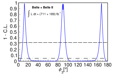
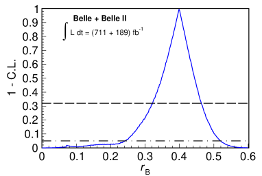
Figure 7: $p$-values ($1-\text{CL}$) as functions of $\phi_{3}$ (left) and $r_{B}$ (right). The dashed horizontal line shows the 68.3% CL, and the dash-dotted line shows the 95.4% CL.

7 Conclusion

We measure the $C\!P$ asymmetries and ratios of branching-fraction ratios for $B^{\pm}\rightarrow D_{C\!P\pm}K^{\pm}$ for the $C\!P$-odd $D$ final state $K^{+}K^{-}$ and the $C\!P$-even final state $K^{0}_{\rm\scriptscriptstyle S}\pi^{0}$ with a combined analysis of the full Belle data set of $772\text{\times}{10}^{6}$ $B\kern 1.79993pt\overline{\kern-1.79993ptB}{}$ pairs and a Belle II data set containing $198\text{\times}{10}^{6}$ $B\kern 1.79993pt\overline{\kern-1.79993ptB}{}$ pairs. As expected, the asymmetries have opposite signs, showing prominent $C\!P$ violation in $B^{\pm}\rightarrow D_{C\!P}K^{\pm}$. The statistical and systematic precision of our results, based on a data set almost four times larger than the previous Belle measurement GLW_Belle , is significantly improved. The results are consistent with those of the BABAR and LHCb experiments babar_paper ; lhcb_paper . We obtain 68.3%-CL intervals for the CKM angle $\phi_{3}$ and the amplitude ratio $r_{B}$:

$$\phi_{3} \in[8.5^{\circ},16.5^{\circ}]\cup[84.5^{\circ},95.5^{\circ}]\cup[163.3^{\circ},171.5^{\circ}],$$ (17)

$$r_{B} \in[0.321,0.465].$$ (18)

Appendix A Correlation matrices

Table 4 and 5 list the statistical and systematic correlation matrices for $\mathcal{A}_{C\!P\pm}$ and $\mathcal{R}_{C\!P\pm}$. We vary every fixed parameter randomly by Gaussian distribution for thousand times. We repeat the fit with the varied values for every fixed parameter, which can result in Gaussian-like distributions of the measured observables. The correlations are calculated by using those Gaussian-like distributions. These correlation matrices are used in the extraction of $\phi_{3}$, $\delta_{B}$ and $r_{B}$.

Table 4: Statistical correlation matrix of measured observables.

	$\mathcal{R}_{C\!P+}$	$\mathcal{R}_{C\!P-}$	$\mathcal{A}_{C\!P+}$	$\mathcal{A}_{C\!P-}$
$\mathcal{R}_{C\!P+}$	1	$-0.081$	0.060	0.000
$\mathcal{R}_{C\!P-}$		1	0.000	0.056
$\mathcal{A}_{C\!P+}$			1	0.000
$\mathcal{A}_{C\!P-}$				1

Table 5: Systematic correlation matrix of measured observables.

	$\mathcal{R}_{C\!P+}$	$\mathcal{R}_{C\!P-}$	$\mathcal{A}_{C\!P+}$	$\mathcal{A}_{C\!P-}$
$\mathcal{R}_{C\!P+}$	1	$-0.063$	$0.342$	$0.005$
$\mathcal{R}_{C\!P-}$		1	$-0.128$	$-0.490$
$\mathcal{A}_{C\!P+}$			1	$0.542$
$\mathcal{A}_{C\!P-}$				1

Appendix B $D$ mass sidebands for the $B^{\pm}\rightarrow D_{C\!P+}K^{\pm}$ mode

In Section 4, we use eight $D$ mass sidebands of data to estimate the peaking background for the $D_{C\!P+}$ mode. Table 6 lists the sideband mass ranges used in the Belle and Belle II analyses, respectively. These sidebands are chosen to extend over the same range as the signal $D$ region.

Table 6: $D$ sideband mass regions for $D_{C\!P+}$ mode, in GeV/$c^{2}$ units.

Analysis	Lower sidebands	Upper sidebands
Belle	[1.67,1.71][1.71,1.75]	[1.90,1.94][1.94,1.98]
	[1.75,1.79][1.79,1.83]	[1.98,2.02][2.02,2.06]
Belle II	[1.706,1.732][1.732,1.758]	[1.758,1.784][1.784,1.810]
	[1.920,1.946][1.946,1.972]	[1.972,1.998][1.998,2.024]

Fig 8 shows distributions and fit-result projections in the data sidebands for the Belle analysis. We obtain the peaking background yield for each sideband and interpolate those yields linearly.

The Belle II data sample used in this analysis has only an integrated luminosity of $189\text{\,}\mathrm{f}\mathrm{b}^{-1}$, which is insufficient to estimate the yield of peaking background. Instead we obtain the Belle II yield by scaling the Belle yield by the reconstruction efficiencies $\epsilon$ of $B^{-}\rightarrow K^{-}K^{+}K^{-}$ in simulated data and the luminosities ($L$) of Belle and Belle II data samples:

$$Y_{B2}(B^{-}\rightarrow K^{-}K^{+}K^{-})=Y_{B}(B^{-}\rightarrow K^{-}K^{+}K^{-})\frac{\epsilon_{B2}L_{B2}}{\epsilon_{B}L_{B}},$$ (19)

where subscripts $B$ and $B2$ stand for Belle and Belle II, respectively.

\begin{overpic}[width=199.4681pt]{figures/appendix/Bdata_KK_SB1_Fit.pdf} \put(87.0,59.0){(a)} \end{overpic}

\begin{overpic}[width=199.4681pt]{figures/appendix/Bdata_KK_SB2_Fit.pdf} \put(87.0,59.0){(b)} \end{overpic}

\begin{overpic}[width=199.4681pt]{figures/appendix/Bdata_KK_SB3_Fit.pdf} \put(87.0,59.0){(c)} \end{overpic}

\begin{overpic}[width=199.4681pt]{figures/appendix/Bdata_KK_SB4_Fit.pdf} \put(87.0,59.0){(d)} \end{overpic}

\begin{overpic}[width=199.4681pt]{figures/appendix/Bdata_KK_SB5_Fit.pdf} \put(87.0,59.0){(e)} \end{overpic}

\begin{overpic}[width=199.4681pt]{figures/appendix/Bdata_KK_SB6_Fit.pdf} \put(87.0,59.0){(f)} \end{overpic}

\begin{overpic}[width=199.4681pt]{figures/appendix/Bdata_KK_SB7_Fit.pdf} \put(87.0,59.0){(g)} \end{overpic}

\begin{overpic}[width=199.4681pt]{figures/appendix/Bdata_KK_SB8_Fit.pdf} \put(87.0,59.0){(h)} \end{overpic}

Figure 8: $\Delta E$ distributions of $B^{\pm}\rightarrow D(\rightarrow K^{-}K^{+})K^{\pm}$ in Belle data with the fit projections overlaid for the lower sidebands [1.67, 1.71] $\mathrm{GeV}/c^{2}$ (a), [1.71, 1.75] $\mathrm{GeV}/c^{2}$ (b), [1.75, 1.79] $\mathrm{GeV}/c^{2}$ (c), and [1.79, 1.83] $\mathrm{GeV}/c^{2}$ (d), and the upper sidebands [1.90, 1.94] $\mathrm{GeV}/c^{2}$ (e), [1.94, 1.98] $\mathrm{GeV}/c^{2}$ (f), [1.98, 2.02] $\mathrm{GeV}/c^{2}$ (g), and [2.02, 2.06] $\mathrm{GeV}/c^{2}$ (h).

References

- (1) N. Cabibbo, Unitary Symmetry and Leptonic Decays, Phys. Rev. Lett. 10, 531 (1963) .
- (2) M. Kobayashi and T. Maskawa, CP violation in the renormalizable theory of weak interaction, Prog. Theor. Phys. 49, 652 (1973).
- (3) M. Gronau and D. London, How to determine all the angles of the unitarity triangle from and , Phys. Lett. B 253, 483 (1991) .
- (4) M. Gronau and D. Wyler, On determining a weak phase from charged B decay asymmetries, Phys. Lett. B 265, 172 (1991).
- (5) M. Rama, Effect of - mixing in the extraction of with and decays, Phys. Rev. D 89, 014021 (2014).
- (6) R. L. Workman et al. (Particle Data Group), Review of Particle Physics, Prog. Theor. Exp. Phys. 2022, 083C01 (2022) and 2023 update.
- (7) Y. Amhis et al. (Heavy Flavor Averaging Group collaboration), Averages of -hadron, -hadron, and -lepton properties as of 2021, Phys. Rev. D 107, 052008 (2023).
- (8) R. Aaij et al., LHCb collaboration, Simultaneous determination of the CKM angle and parameters related to mixing and violation in the charm sector, LHCb-CONF-2022-003.
- (9) D. Atwood, I. Dunietz, and A. Soni, Enhanced CP violation with modes and extraction of the CKM angle , Phys. Rev. Lett. 78, 3257 (1997).
- (10) D. Atwood, I. Dunietz, and A. Soni, Improved methods for observing CP violation in and measuring the CKM phase , Phys. Rev. D 63, 036005 (2001).
- (11) Y. Horii et al., Belle collaboration, Evidence for the Suppressed Decay , Phys. Rev. Lett. 106, 231803 (2011).
- (12) A. Giri, Y. Grossman, A. Soffer, and J. Zupan, Determining using with multibody decays, Phys. Rev. D 68, 054018 (2003).
- (13) A. Bondar, Proceedings of BINP Special Analysis Meeting on Dalitz Analysis, (unpublished) 2002.
- (14) F. Abudinen et al., Belle and Belle II collaborations, Combined analysis of Belle and Belle II data to determine the CKM angle using decays, J. High Energy Phys. 63 (2022).
- (15) K. Abe et al., Belle collaboration, Study of and decays, Phys. Rev. D 73, 051106 (2006).
- (16) S. Kurokawa and E. Kikutani, Overview of the KEKB accelerators, Nucl. Instrum. Meth. A 499, 1 (2003).
- (17) T. Abe et al., Achievement of the KEKB, Prog. Theor. Exp. Phys. (2013) 03A001-03A011.
- (18) K. Akai, K. Furukawa, and H. Koiso, SuperKEKB Collider, Nucl. Instrum. Meth. A 907 (2018) 188.
- (19) A. Abashian et al., Belle collaboration, The Belle Detector, Nucl. Instrum. Meth. A 479, (2002) 117.
- (20) J. Brodzicka et al., Physics Achievements from the Belle Experiment, Prog. Theor. Exp. Phys. (2012) 04D001.
- (21) T. Abe et al., Belle II collaboration, Belle II Technical Design Report, [arXiv:1101.0352].
- (22) D. J. Lange, The EvtGen particle decay simulation package, Nucl. Instrum. Meth. A 462, (2001) 152.
- (23) B. Ward, S. Jadach and Z. Wa̧s, Precision calculation for : The KK MC project, Nucl. Phys. B Proc. Suppl. 116 (2003) 73.
- (24) T. Sjstrand et al., A Brief Introduction to Pythia 8.1 , Comput. Phys. Commun. 178 (2008) 852.
- (25) R. Brun et al., GEANT 3.21, CERN-DD-EE-84-01 (1984) [inSPIRE].
- (26) S. Agostinelli et al., GEANT4 - a simulation toolkit, Nucl. Instrum. Meth. A 506 (2003) 250.
- (27) E. Barberio and Z. Wa̧s, PHOTOS: A Universal Monte Carlo for QED radiative corrections, Comp. Phys. Commun. 79, 291 (1994).
- (28) T. Kuhr et al., The Belle II Core Software, Comput. Softw. Big Sci. 3 (2019) 1.
- (29) “Belle II Analysis Software Framework (basf2), https://doi.org/10.5281/zenodo.5574115.” 10.5281/zenodo.5574115.
- (30) M. Gelb et al., B2BII: Data Conversion from Belle to Belle II, Comput. Softw. Big Sci. 2 (2018) 9.
- (31) F. Abudinen et al., Belle II collaboration, Study of decays using of Belle II data, [arXiv:2104.03628].
- (32) H. Nakano et al., Search for new physics by a time-dependent CP violation analysis of the decay using the Belle detector, Ph.D Thesis, Tohoku University (2014), unpublished. [Thesis].
- (33) H. Nakano et al., Measurement of time-dependent CP asymmetries in decays, Phys. Rev. D 97, 092003 (2018).
- (34) G. C. Fox and S. Wolfram, Observables for the Analysis of Event Shapes in Annihilation and Other Processes, Phys. Rev. Lett. 41, 1581 (1978).
- (35) S. H. Lee et al., Belle collaboration, Evidence for , Phys. Rev. Lett. 91, 261801 (2003).
- (36) H. Kakuno et al., Belle collaboration, Neutral B Flavor Tagging for the Measurement of Mixing-induced CP Violation at Belle, Nucl. Instrum. Meth. A 533, 516 (2004).
- (37) F. Abudinén et al., B-flavor tagging at Belle II, Eur. Phys. J. C 82, 283 (2022).
- (38) A. Hocker et al., TMVA- Toolkit for Multivariate Data Analysis, arXiv:physics/0703039.
- (39) H. Ikeda et al., Belle collaboration, A detailed test of the CsI(T) calorimeter for BELLE with photon beams of energy between 20 MeV and 5.4 GeV, Nucl. Instrum. Meth. A 441, 401 (2000).
- (40) E. Nakano, Belle PID, Nucl. Instrum. Meth. A 494, 402 (2002).
- (41) J. Charles et al., CKMfitter collaboration, CP Violation and the CKM Matrix: Assessing the Impact of the Asymmetric B Factories, Eur. Phys. J. C 41, 1-131 (2005) [ online update].
- (42) P. del Amo Sanchez et al., BaBar collaboration, Measurement of CP observables in decays and constraints on the CKM angle , Phys. Rev. D 82 072004 (2010).
- (43) R. Aaji et al., LHCb collaboration, Measurement of CP observables in and decays using two-body D final states , J. High Energy Phys. 81 (2021).