Feature Modulation Transformer: Cross-Refinement of Global Representation via High-Frequency Prior for Image Super-Resolution

Abstract

Transformer-based methods have exhibited remarkable potential in single image super-resolution (SISR) by effectively extracting long-range dependencies. However, most of the current research in this area has prioritized the design of transformer blocks to capture global information, while overlooking the importance of incorporating high-frequency priors, which we believe could be beneficial. In our study, we conducted a series of experiments and found that transformer structures are more adept at capturing low-frequency information, but have limited capacity in constructing high-frequency representations when compared to their convolutional counterparts. Our proposed solution, the cross-refinement adaptive feature modulation transformer (CRAFT), integrates the strengths of both convolutional and transformer structures. It comprises three key components: the high-frequency enhancement residual block (HFERB) for extracting high-frequency information, the shift rectangle window attention block (SRWAB) for capturing global information, and the hybrid fusion block (HFB) for refining the global representation. Our experiments on multiple datasets demonstrate that CRAFT outperforms state-of-the-art methods by up to 0.29dB while using fewer parameters. The source code will be made available at: https://github.com/AVC2-UESTC/CRAFT-SR.git.

1 Introduction

Single image super-resolution (SISR) has garnered significant attention in recent years, owing to its promising applications across diverse domains, such as surveillance video and medical image enhancement [31, 10], old image reconstruction [21, 17], and efficient image transmission [47]. Despite its practical value, SISR remains an ill-posed problem, given the existence of multiple solutions for a given low-resolution (LR) image. To tackle this challenge, a multitude of classical approaches have been proposed, including A+ [36], SC [41], and ANR [35]. However, these methods exhibit limitations in their performance, primarily attributed to their constrained model capacities.

In recent years, deep learning has experienced significant growth and demonstrated remarkable success in SISR [7, 20, 45, 22]. Prior research efforts have introduced residual and dense connectives to facilitate the stacking of deep convolutional neural networks (CNNs) [16, 37], while others [46, 40, 29, 30] have leveraged attention mechanisms to enhance performance. Notably, the emergence of transformer architectures has demonstrated their efficacy in capturing long-range dependencies and attaining state-of-the-art performance [21, 6, 4, 18, 25]. Despite these advancements, these works have mainly focused on designing transformer blocks to obtain global information and overlooked the potential of incorporating high-frequency priors [32, 8] to further bolster performance in SISR. Additionally, there is limited detailed analysis of the impact of frequency on performance.

In this paper, we investigate the influence of high-frequency information on the performance of CNN and transformer structures in SISR. We achieve this by discarding different ratios of high-frequency components from the input image and observing the corresponding performance changes. Our empirical findings reveal that transformers tend to prioritize low-frequency information and exhibit limited capability in constructing high-frequency representations when compared to CNNs. To address this issue, we proposed a cross-refinement adaptive feature modulation transformer (CRAFT) that integrates the strengths of both structures. Specifically, CRAFT comprises three key components, namely the high-frequency enhancement residual block (HFERB), the shift rectangle window attention block (SRWAB), and the hybrid fusion block (HFB), which work collaboratively to capture high-frequency details, extract long-range dependencies, and refine the output for better representation. Experimental results show that CRAFT outperforms state-of-the-art performance with relatively fewer parameters. The main contributions of this paper are as follows:

• We study the impact of CNN and transformer structures on performance from a frequency perspective and observe that transformer is more effective in capturing low-frequency information while having limited capacity for constructing high-frequency representations compared to CNN.

• Based on the observation, we design a parallel structure to explore different frequency features. We utilize the HFERB branch to introduce high-frequency information, which is beneficial to SISR, and the SRWAB branch to acquire global information.

• We propose a fuse strategy that integrates the strengths of CNN and transformer. Specifically, we treat the HFERB branch as high-frequency prior and the output of SRWAB as key and value for inter-attention, resulting in improved performance.

• Extensive experimental results on multiple datasets show that the proposed method performs on par with the existing state-of-the-art SISR methods while using fewer parameters.

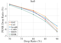
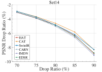
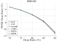
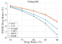
(a) Dependency of different structures on high-frequency information.

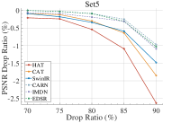
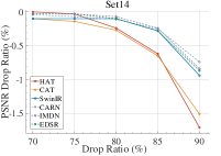
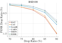
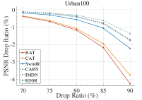
(b) Effectiveness of reconstructing high-frequency information.

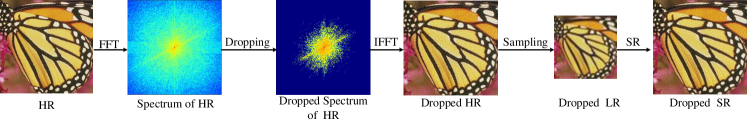
(c) The procedure of dropping high-frequency.

Figure 1: The influence of high-frequency information on the performance of CNN and transformer architectures. Dashed and solid lines correspond to CNN and transformer methods, respectively. (a) With an increase in the high-frequency drop ratio, transformer models exhibit a smaller change in PSNR compared to CNN, suggesting their superiority in capturing low-frequency information. (b) As the high-frequency drop ratio increases, transformer models show a more pronounced change in PSNR compared to CNN, indicating their limited ability to reconstruct high-frequency information from low-frequency.

2 Related Works

2.1 CNN-based SISR

Since the pioneering work SRCNN [7] has achieved significant progress in SISR, various CNN-based works have been proposed. Kim et al. [15] presented an SR method using deep networks by cascading 20 layers, demonstrating promising results. Building upon this, Lim et al. [23] introduced the enhanced deep super-resolution (EDSR) network, which achieved a significant performance boost by removing the batch normalization layer [14] from the residual block and incorporating additional convolution layers. Ahn et al. [2] designed an architecture with an increased number of residual blocks and dense connections, further improving the SR performance. In pursuit of lightweight models, Hui et al. [13] proposed a selective fusion approach, employing cascaded information multi-distillation blocks to construct an efficient model. Li et al. [19] introduced a method involving predefined filters and utilized a CNN to learn coefficients, which were then linearly combined to obtain the final results. Sun et al. [34] proposed a hybrid pixel-unshuffled network (HPUN) by introducing an efficient and effective downsampling module into the SR task.

2.2 Transformer-based SISR

Liang et al. [21] proposed SwinIR, a robust baseline model for image restoration, leveraging the Swin Transformer [24]. CAT [6] modified the window shape and introduced a rectangle window attention to obtaining better performance. Chen et al. [4] proposed a pre-trained image processing transformer and showed that pre-trained mechanism could significantly improve the performance for low-level tasks. Li et al. [18] comprehensively analyzed the effect of pre-training and proposed a versatile model to tackle different low-level tasks. Lu et al. [25] proposed a lightweight transformer to capture long-range dependencies between similar patches in an image with the help of the specially designed efficient transformer and efficient attention mechanism. Zhang et al. [44] introduced a shift convolution and a group-wise multi-scale self-attention to reduce the complexity of transformer. HAT [5] introduced a hybrid attention mechanism to enhance the performance of window-based transformers.

3 Analysis of Frequency Impact

This section delves into the influence of performance from a frequency perspective. To analyze the impact of various frequencies on CNN and transformer, we conduct two sets of experiments using four common used benchmarks, as illustrated in Figure 1.

We select CARN [2], IMDN [13], EDSR [23], and SwinIR [21], CAT [6], HAT [5] as representatives of CNN and transformer structures. The process of dropping frequency components is depicted in Figure 1(c). Given a high-resolution (HR) image $X^{HR}$, we perform a fast Fourier transform (FFT) on it to obtain its frequency spectrum. Subsequently, we flatten this spectrum into a sequence and arrange it in ascending order based on the magnitudes. With a sequence length of $L$, we define a threshold determined by the drop ratio $\gamma$, $0\leq\gamma\leq 1$, located at the magnitude corresponding to the position $\gamma\cdot L$. Frequency components with magnitudes below this threshold are set to zero. Following this, we perform an inverse fast Fourier transform (IFFT) to generate the HR image with dropped frequencies, referred to as $X_{drop}^{HR}(\gamma)$. The formulation for this process is as follows

$$X_{drop}^{HR}(\gamma)=IFFT(Drop(|FFT(X^{HR})|,\gamma)).$$ (1)

Afterward, we downsample $X_{drop}^{HR}(\gamma)$ using bicubic interpolation to obtain the LR version $X_{drop}^{LR}(\gamma)$ (e.g. $\times 4$ down-sampling). Finally, we employ CNN-based and transformer-based SR models to generate the super-resolved counterpart $X_{drop}^{SR}(\gamma)$.

To analyze the dependency of CNN and transformer on high-frequency information, we compute the peak signal-to-noise ratio (PSNR) $P^{D}(\gamma)$ between $X_{drop}^{SR}(\gamma)$ and $X_{drop}^{HR}$. We then plot the PSNR drop trend to visualize the difference between the two structures. As shown in Figure 1(a), the PSNR drop ratio for each drop ratio is defined as

$$R_{drop}^{D}(\gamma)=\frac{P(0)-P^{D}(\gamma)}{P(0)},$$ (2)

where $P(0)$ represents the PSNR without dropping, calculated between $X^{SR}$ and $X^{HR}$. The figures illustrate that the transformer model exhibits reduced sensitivity to high-frequency information and excels in capturing low-frequency information, as evidenced by the smaller PSNR change compared to the CNN model as the proportion of discarded high-frequency information increases.

Furthermore, we conduct another experiment to evaluate the effectiveness of different structures in reconstructing high-frequency information. Specifically, we calculate the PSNR $P^{E}(\gamma)$ between $X_{drop}^{SR}(\gamma)$ and $X^{HR}$ and plot the performance drop trend as previously depicted. The PSNR drop ratio for each drop ratio can be expressed as

$$R_{drop}^{E}(\gamma)=\frac{P^{E}(\gamma)-P(0)}{P(0)}.$$ (3)

From Figure 1(b), we observe that as the proportion of discarded high-frequency information increases, the transformer model experiences a larger PSNR change compared to the CNN model, indicating its limited ability to reconstruct high-frequency information from low-frequency.

Based on these observations, we argue that the transformer requires the assistance of CNN to enhance its capability to recover intricate details. To address this, we propose a method that combines the strengths of both CNN and transformer. Specifically, we introduce CNN information as a high-frequency prior to aid the transformer in refining the global representation.

4 Proposed Method

\begin{overpic}[scale={.35}]{figs/camera_ready/craft.pdf} \put(1.5,51.5){\footnotesize{$X_{\scriptscriptstyle H}$}} \put(18.8,51.5){\footnotesize{$X_{\scriptscriptstyle S}$}} \put(1.5,25.5){\footnotesize{$X_{\scriptscriptstyle H}$}} \put(1.5,15.5){\footnotesize{$X_{\scriptscriptstyle S}$}} \par\put(12.0,55.0){\footnotesize{C}} \put(12.0,34.0){\footnotesize{C}} \put(3.0,40.0){\footnotesize{C}} \put(19.0,37.0){\footnotesize{C}} \par\par\put(25.5,46.3){\footnotesize{C}} \put(27.9,53.0){\footnotesize{C/2}} \put(27.9,37.5){\footnotesize{C/2}} \par\put(20.2,25.5){\footnotesize{${\boldsymbol{\hat{Q}}}$}} \put(24.0,15.8){\footnotesize{${\boldsymbol{\hat{K}}}$}} \put(24.0,6.3){\footnotesize{${\boldsymbol{\hat{V}}}$}} \par\end{overpic}

Figure 2: The framework of CRAFT. HFERB extracts the high frequency from the input features, SRWAB captures the long-range dependency of input features, and HFB integrates the output of HFERB and SRWAB to cross refine the global features. Best viewed in color.

The CRAFT network comprises three key components: Shallow feature extraction, residual cross-refinement fusion groups (RCRFGs), and reconstruction as shown in Figure 2. The shallow feature extraction module comprises a single convolutional layer, while the reconstruction module is followed by the SwinIR [21]. The RCRFG component consists of several cross-refinement fusion blocks (CRFBs), each comprising three types of blocks: the high-frequency enhancement residual blocks (HFERBs), the shift rectangle window attention blocks (SRWABs), and the hybrid fusion blocks (HFBs). We first describe the overall structure of CRAFT and then elaborate on the three key designs, including HFERB, SRWAB, and HFB.

4.1 Model Overview

The input LR image is processed by a $3\times 3$ convolutional layer to obtain shallow features. These features are then fed into a serial of RCRFGs to learn deep features. After the last RCRFG, a $3\times 3$ convolutional layer aggregates the features, and a residual connection is established between its output and the shallow features for facilitating training. The reconstruction module employs a $3\times 3$ convolutional layer to aggregate the features, and a shuffle layer [33] is used to obtain the final SR output image.

4.2 High-frequency Enhancement Residual Block

The HFERB aims to enhance the high-frequency information, as shown in Figure 2. It comprises the local feature extraction (LFE) branch and the high-frequency enhancement (HFE) branch. Specifically, we split the input features $F_{in}\in\mathbb{R}^{H\times W\times C}$ into two parts, and then processed by the two branches separately

$$F_{in}^{LFE},F_{in}^{HFE}=Split(F_{in}),$$ (4)

where $F_{in}^{LFE},F_{in}^{HFE}\in\mathbb{R}^{H\times W\times C/2}$ represent the input of LFE and HFE. For the LFE branch, we utilize a $3\times 3$ convolutional layer followed by a GELU activation function to extract local high-frequency features

$$\hat{F}_{in}^{LFE}=f_{a}(Conv_{3\times 3}(F_{in}^{LFE})),$$ (5)

where the $Conv_{3\times 3}(\cdot)$ refers to the convolutional layer and the $f_{a}(\cdot)$ represents the GELU activation layer. For the HFE branch, we employ a max-pooling layer to extract high-frequency information from the input features $F_{in}^{HFE}$. Then, we use a $1\times 1$ convolutional layer followed by a GELU activation function to enhance the high-frequency features,

$$\hat{F}_{in}^{HFE}=f_{a}(Conv_{1\times 1}(MaxPooling(F_{in}^{HFE}))),$$ (6)

where the $Conv_{1\times 1}(\cdot)$ indicates the convolutional layer, the $MaxPooling(\cdot)$ means the max-pooling layer and the $f_{a}(\cdot)$ represents the GELU activation layer. The outputs of the two branches are then concatenated and fed into a $1\times 1$ convolutional layer to fuse the information thoroughly. To make the network benefit from multi-scale information and maintain training stability, a skip connection is introduced. The whole process can be formulated as

$$X_{H}=Conv_{1\times 1}(Concat(\hat{F}_{in}^{LFE},\hat{F}_{in}^{HFE}))+F_{in},$$ (7)

where the $Concat(\cdot)$ refers to the concatenation operation and the $Conv_{1\times 1}(\cdot)$ represents the convolutional layer.

4.3 Shift Rectangle Window Attention Block

We utilize the shift rectangle window (SRWin) to expand the receptive field, which can benefit SISR [6]. Unlike square windows, the SRWin uses rectangle windows to capture more relevant information along the longer axis. In detail, given an input $X_{in}\in\mathbb{R}^{H\times W\times C}$, we divide it into $\frac{H\times W}{rh\times rw}$ rectangle windows, where $rh$ and $rw$ refer to the height and width of the rectangle window. For the $i$-th rectangle window feature $X_{i}\in\mathbb{R}^{(rh\times rw)\times C}$, we compute the query, key, and value as follows

$$\boldsymbol{Q}_{i}=X_{i}W_{i}^{Q},\boldsymbol{K}_{i}=X_{i}W_{i}^{K},\boldsymbol{V}_{i}=X_{i}W_{i}^{V},$$ (8)

where the $W_{i}^{Q}\in\mathbb{R}^{C\times d}$, $W_{i}^{K}\in\mathbb{R}^{C\times d}$ and $W_{i}^{V}\in\mathbb{R}^{C\times d}$ represent the projection matrices and $d$ is projection dimension which is commonly set to $d=\frac{C}{M}$ where the $M$ is the number of heads. The self-attention can be formulated as

$$Attention(\boldsymbol{Q}_{i},\boldsymbol{K}_{i},\boldsymbol{V}_{i})=Softmax(\frac{\boldsymbol{Q}_{i}\boldsymbol{K}_{i}^{T}}{\sqrt{d}}+B)\boldsymbol{V}_{i},$$ (9)

where $B$ is the dynamic relative position encoding [38]. Moreover, a convolutional operation on the value is introduced to enhance local extraction capability. To capture information from different axes, we utilize two types of rectangle windows: Horizontal and vertical windows. Unlike traditional operations that utilize attention masks to limit calculations to the same window, in practice, we eliminate the mask and enable more extensive information interaction across different windows. Accordingly, we split the attention heads into two equal groups and compute the self-attention within each group separately. We then concatenate the outputs of the two groups to obtain the final output. The procedure can be expressed as

$$Rwin\mbox{-}SA(X)=Concat(V\mbox{-}Rwin,H\mbox{-}Rwin)W^{p},$$ (10)

where the $W^{p}\in\mathbb{R}^{C\times C}$ represents the linear projection to fuse the features, $V\mbox{-}Rwin$ and $H\mbox{-}Rwin$ indicate the vertical and horizontal rectangle window attention. In addition, a multi-layer perceptron (MLP) is used for further feature transformations. The whole process can be formulated as

$$\begin{split}&X=Rwin\mbox{-}SA(LN(X_{in}))+X_{in}\\ &X_{S}=MLP(LN(X))+X,\end{split}$$ (11)

where the $LN$ represents the LayerNorm layer.

4.4 Hybrid Fusion Block

To better integrate the merits of CNN and transformer (HFERB and SRWAB), we have designed a hybrid fusion block (HFB), which is illustrated in Figure 2. We formulate the output of HFERB as the high frequency prior query and the output of SRWAB as key, value and calculate the inter-attention to refine the global features which are obtained from SRWAB. Moreover, most existing methods focus on spatial relations and overlook channel information. To overcome this limitation, we perform inter-attention based on the channel dimension to explore channel dependencies. This design will significantly reduce complexity. Traditional methods that utilize spatial attention tend to result in significant computational complexity (e.g., $O(N^{2}C),N\gg C$), where $N$ represents the length of the sequence and $C$ represents the channel dimension. In contrast, our channel attention design can transfer the quadratic component to the channel dimension (e.g., $O(NC^{2})$), effectively reducing complexity.

Table 1: Performance comparison of different SISR models on five benchmarks. Params represents the total number of network parameters. Results for the best and second best candidates are highlighted, and underlined.

Scale	Model	Params	Set5 (PSNR/SSIM)	Set14 (PSNR/SSIM)	BSD100 (PSNR/SSIM)	Urban100 (PSNR/SSIM)	Manga109 (PSNR/SSIM)
${\times 2}$	EDSR-baseline [23]	1370K	37.99/0.9604	33.57/0.9175	32.16/0.8994	31.98/0.9272	38.54/0.9769
	CARN [2]	1592K	37.76/0.9590	33.52/0.9166	32.09/0.8978	31.92/0.9256	38.36/0.9765
	IMDN [13]	694K	38.00/0.9605	33.63/0.9177	32.19/0.8996	32.17/0.9283	38.88/0.9774
	LatticeNet [26]	756K	38.06/0.9607	33.70/0.9187	32.20/0.8999	32.25/0.9288	-/-
	LAPAR-A [19]	548k	38.01/0.9605	33.62/0.9183	32.19/0.8999	32.10/0.9283	38.67/0.9772
	HPUN-L [34]	714K	38.09/0.9608	33.79/0.9198	32.25/0.9006	32.37/0.9307	39.07/0.9779
2-8[1pt/1pt]	SwinIR-light [21]	878K	38.14/0.9611	33.86/0.9206	32.31/0.9012	32.76/0.9340	39.12/0.9783
	ESRT [25]	777K	38.03/0.9600	33.75/0.9184	32.25/0.9001	32.58/0.9318	39.12/0.9774
	ELAN-light [44]	582K	38.17/0.9611	33.94/0.9207	32.30/0.9012	32.76/0.9340	39.11/0.9782
	CRAFT (Ours)	737K	38.23/0.9615	33.92/0.9211	32.33/0.9016	32.86/0.9343	39.39/0.9786
${\times 3}$	EDSR-baseline [23]	1555K	34.37/0.9270	30.28/0.8417	29.09/0.8052	28.15/0.8527	33.45/0.9439
	CARN [2]	1592K	34.29/0.9255	30.29/0.8407	29.06/0.8034	28.06/0.8493	33.50/0.9440
	IMDN [13]	703K	34.36/0.9270	30.32/0.8417	29.09/0.8046	28.17/0.8519	33.61/0.9445
	LatticeNet [26]	765K	34.53/0.9281	30.39/0.8424	29.15/0.8059	28.33/0.8538	-/-
	LAPAR-A [19]	544k	34.36/0.9267	30.34/0.8421	29.11/0.8054	28.15/0.8523	33.51/0.9441
	HPUN-L [34]	723K	34.56/0.9281	30.45/0.8445	29.18/0.8072	28.37/0.8572	33.90/0.9463
2-8[1pt/1pt]	SwinIR-light [21]	886K	34.62/0.9289	30.54/0.8463	29.20/0.8082	28.66/0.8624	33.98/0.9478
	LBNet [9]	736K	34.47/0.277	30.38/0.8417	29.13/0.8061	28.42/0.8559	33.82/0.9406
	ESRT [25]	770K	34.42/0.9268	30.43/0.8433	29.15/0.8063	28.46/0.8574	33.95/0.9455
	ELAN-light [44]	590K	34.61/0.9288	30.55/0.8463	29.21/0.8081	28.69/0.8624	34.00/0.9478
	CRAFT (Ours)	744K	34.71/0.9295	30.61/0.8469	29.24/0.8093	28.77/0.8635	34.29/0.9491
${\times 4}$	EDSR-baseline [23]	1518K	32.09/0.8938	28.58/0.7813	27.57/0.7357	26.04/0.7849	30.35/0.9067
	CARN [2]	1592K	32.13/0.8937	28.60/0.7806	27.58/0.7349	26.07/0.7837	30.47/0.9084
	IMDN [13]	715K	32.21/0.8948	28.58/0.7811	27.56/0.7353	26.04/0.7838	30.45/0.9075
	LatticeNet [26]	777K	32.18/0.8943	28.61/0.7812	27.57/0.7355	26.14/0.7844	-/-
	LAPAR-A [19]	659k	32.15/0.8944	28.61/0.7818	27.61/0.7366	26.14/0.7871	30.42/0.9074
	HPUN-L [34]	734K	32.31/0.8962	28.73/0.7842	27.66/0.7386	26.27/0.7918	30.77/0.9109
2-8[1pt/1pt]	SwinIR-light [21]	897K	32.44/0.8976	28.77/0.7858	27.69/0.7406	26.47/0.7980	30.92/0.9151
	LBNet [9]	742K	32.29/0.8960	28.68/0.7832	27.62/0.7382	26.27/0.7906	30.76/0.9111
	ESRT [25]	751K	32.19/0.8947	28.69/0.7833	27.69/0.7379	26.39/0.7962	30.75/0.9100
	ELAN-light [44]	601K	32.43/0.8975	28.78/0.7858	27.69/0.7406	26.54/0.7982	30.92/0.9150
	CRAFT (Ours)	753K	32.52/0.8989	28.85/0.7872	27.72/0.7418	26.56/0.7995	31.18/0.9168

Specifically, as shown in Figure 2, we use a $1\times 1$ convolutional layer followed by a $3\times 3$ depth-wise convolutional layer to generate the high frequency query $\boldsymbol{Q}\in\mathbb{R}^{H\times W\times C}$ based on the output of HFERB, $X_{H}$. As to the output of SRWAB, $X_{S}$, we first normalize the features by LayerNorm layer and then use the same operation as the query $\boldsymbol{Q}$ to get the key $\boldsymbol{K}\in\mathbb{R}^{H\times W\times C}$ and the value $\boldsymbol{V}\in\mathbb{R}^{H\times W\times C}$. Following the [42], we perform the reshape operation on $\boldsymbol{Q}$, $\boldsymbol{K}$ and $\boldsymbol{V}$ to get the $\boldsymbol{\hat{Q}}\in\mathbb{R}^{C\times(HW)}$, $\boldsymbol{\hat{K}}\in\mathbb{R}^{C\times(HW)}$ and $\boldsymbol{\hat{V}}\in\mathbb{R}^{C\times(HW)}$. After that, we compute the inter-attention as

$$Attention(\boldsymbol{\hat{Q}},\boldsymbol{\hat{K}},\boldsymbol{\hat{V}})=Softmax(\frac{\boldsymbol{\hat{Q}}\boldsymbol{\hat{K}^{T}}}{\alpha})\boldsymbol{\hat{V}},$$ (12)

where the $\alpha$ represents the learnable parameter. Meanwhile, we add the refinement features to the $X_{S}$ to get the fusion output $X_{fuse}$. In addition, we feed $X_{fuse}$ to an improved feed-forward network [42] to aggregate the features further. The details of this structure are shown in Figure 2. It introduced a gate mechanism to fully extract the spatial and channel information and gain better performance. The whole process can be formulated as

$$\begin{split}X_{fuse}&=Inter\mbox{-}Atten(LN(X_{S}),X_{H})+X_{S}\\ X_{HFB}&=IMLP(LN(X))+X_{fuse},\end{split}$$ (13)

where the $LN$ means LayerNorm operation, $IMLP$ represents the improved MLP, and $Inter\mbox{-}Atten$ indicates the proposed inter-attention mechanism, which introduces high-frequency prior to refining the global representations.

5 Experiments

5.1 Data and Metrics

In this paper, we adopt the DIV2K [1] as the training dataset, which includes 800 training images. Meanwhile, five benchmarks are used for evaluation, including Set5 [3], Set14 [43], BSD100 [27], Urban100 [12], and Manga109 [28] with three magnification factors: $\times 2$, $\times 3$, and $\times 4$. The quality of the images is evaluated using PSNR, and SSIM [39]. The complexity of the model is indicated by its parameters.

5.2 Implementation Details

Following the general setting, we use bicubic to obtain the corresponding LR images from the original HR images. During training, we randomly crop the images into $64\times 64$ patches, and the total training iterations are 500K. Meanwhile, data augmentation is performed, such as random horizontal flipping and $90^{\circ}$ rotation. The Adam optimizer with $\beta_{1}=0.9$ and $\beta_{2}=0.999$ is adopted to minimize the $\mathcal{L}_{1}$ Loss. The batch size is set to 64, the initial learning rate is set to $2\times 10^{-4}$ and reduced by half at the milestone [250K, 400K, 450K, 475K]. In addition, the model is trained on 4 NVIDIA 3090 GPUs using the PyTorch toolbox. In CRAFT, we have set the RCRFG number to 4 and the CRFB number to 2 for each RCRFG. Each CRFB is comprised of 1 HFERB and 2 SRWABs for efficiency. The feature channel, attention head, and MLP expansion ratio are set to 48, 6, and 2, respectively. We also set the IMLP expansion ratio to 2.66, as in [42]. To obtain two types of rectangle windows, we have set the rectangle window size to $[sh,sw]$ as $[4,16]$ and $[16,4]$.

5.3 Comparison with state-of-the-art methods

We compare with several state-of-the-art SISR methods to demonstrate the effective of the proposed CRAFT model, including EDSR [23], CARN [2], IMDN [13], LatticeNet [26], LAPAR [19], SwinIR [21], HPUN [34], ESRT [25], LBNet [9], and ELAN [44].

\begin{overpic}[scale={.39}]{figs/camera_ready/ablation_methods.pdf} \put(9.0,46.3){Img012 ($\times 4$)} \put(6.5,23.7){YumeiroCook ($\times 4$)} \put(5.5,1.0){UchuKigekiM774 ($\times 4$)} \par\put(33.7,57.3){Bicubic} \put(51.3,57.3){EDSR~{}\cite[cite]{[\@@bibref{}{Lim2017}{}{}]}} \put(69.8,57.3){CARN~{}\cite[cite]{[\@@bibref{}{Ahn2018}{}{}]}} \put(88.0,57.3){LBNet~{}\cite[cite]{[\@@bibref{}{gao2022lightweight}{}{}]}} \put(32.8,46.3){SwinIR~{}\cite[cite]{[\@@bibref{}{liang2021swinir}{}{}]}} \put(51.3,46.3){ESRT~{}\cite[cite]{[\@@bibref{}{lu2022transformer}{}{}]}} \put(68.5,46.3){CRAFT (Ours)} \put(90.0,46.3){HR} \par\put(33.7,34.8){Bicubic} \put(51.3,34.8){EDSR~{}\cite[cite]{[\@@bibref{}{Lim2017}{}{}]}} \put(69.8,34.8){CARN~{}\cite[cite]{[\@@bibref{}{Ahn2018}{}{}]}} \put(88.0,34.8){LBNet~{}\cite[cite]{[\@@bibref{}{gao2022lightweight}{}{}]}} \put(32.8,23.7){SwinIR~{}\cite[cite]{[\@@bibref{}{liang2021swinir}{}{}]}} \put(51.3,23.7){ESRT~{}\cite[cite]{[\@@bibref{}{lu2022transformer}{}{}]}} \put(68.5,23.7){CRAFT (Ours)} \put(90.0,23.7){HR} \par\put(33.7,12.3){Bicubic} \put(51.3,12.3){EDSR~{}\cite[cite]{[\@@bibref{}{Lim2017}{}{}]}} \put(69.8,12.3){CARN~{}\cite[cite]{[\@@bibref{}{Ahn2018}{}{}]}} \put(88.0,12.3){LBNet~{}\cite[cite]{[\@@bibref{}{gao2022lightweight}{}{}]}} \put(32.8,1.0){SwinIR~{}\cite[cite]{[\@@bibref{}{liang2021swinir}{}{}]}} \put(51.3,1.0){ESRT~{}\cite[cite]{[\@@bibref{}{lu2022transformer}{}{}]}} \put(68.5,1.0){CRAFT (Ours)} \put(90.0,1.0){HR} \end{overpic}

Figure 3: Visual quality comparison with SOTA methods. CRAFT achieves better restoration quality in both line direction and details.

Quantitative Results. The experimental results for SISR are presented in Table 1, where the proposed CRAFT model demonstrates competitive performance across all benchmarks. Particularly, when compared to traditional CNN-based methods like EDSR, the proposed CRAFT achieves significant performance improvements of 0.85dB, 0.84dB, and 0.83dB at magnification factors $\times 2,\times 3$, and $\times 4$, respectively, while using 46%, 52%, and 50% fewer parameters on the Manga109 dataset. Furthermore, compared to recent channel attention methods such as CARN, the proposed CRAFT achieves improvements of 1.03dB, 0.79dB, and 0.71dB at magnification factors $\times 2,\times 3$, and $\times 4$, respectively, with a 54%, 53%, and 52% reduction in the number of parameters on the Manga109 dataset. Regarding transformer-based methods [25, 21, 44], the proposed CRAFT gains performance improvements of 0.34dB, 0.31dB, and 0.29dB, respectively, with a comparable number of parameters under the magnification factor of $\times 3$ on the Manga109 dataset.

Qualitative Results. We present a visual comparison ($\times 4$) in Figure 3 and analyze the results. Our proposed CRAFT model integrates the strengths of both CNN and transformer structures, leading to accurate line direction recovery while preserving image details. To further investigate the performance, we compare the local attribution map (LAM) [11] between CRAFT and SwinIR, as shown in Figure 4. LAM indicates the correlation between the significance of each pixel in LR and the SR of the patch that is outlined with the red box. By leveraging a broader range of information, our model achieves improved results. Furthermore, we examine the diffusion index (DI), which signifies the range of pixels involved. A larger DI indicates a wider scope of attention. Compared to SwinIR, our model exhibits a higher DI, implying that it can capture more contextual information. These results demonstrate the effectiveness of the proposed CRAFT method.

5.4 Ablation study

5.4.1 Effectiveness of HFERB and SRWAB

\begin{overpic}[scale={.3}]{figs/camera_ready/ablation_lam.pdf} \put(5.0,46.3){HR} \put(5.0,31.0){LR} \put(17.5,58.5){SwinIR} \put(25.6,58.5){CRAFT} \put(16.4,31.0){DI: 10.78} \put(24.8,31.0){DI: 30.34} \put(12.6,52.2){\rotatebox{90.0}{\shortstack{LAM\\ Results}}} \put(12.6,41.4){\rotatebox{90.0}{\shortstack{Contribution\\ Area}}} \put(12.6,34.2){\rotatebox{90.0}{\shortstack{SR\\ Results}}} \par\put(39.2,46.3){HR} \put(39.2,31.0){LR} \put(51.3,58.5){SwinIR} \put(59.5,58.5){CRAFT} \put(51.0,31.0){DI: 9.37} \put(58.9,31.0){DI: 30.94} \put(46.6,52.2){\rotatebox{90.0}{\shortstack{LAM\\ Results}}} \put(46.6,41.4){\rotatebox{90.0}{\shortstack{Contribution\\ Area}}} \put(46.6,34.2){\rotatebox{90.0}{\shortstack{SR\\ Results}}} \par\put(73.0,46.3){HR} \put(73.0,31.0){LR} \put(85.4,58.5){SwinIR} \put(93.5,58.5){CRAFT} \put(84.6,31.0){DI: 13.03} \put(92.9,31.0){DI: 30.87} \put(80.6,52.2){\rotatebox{90.0}{\shortstack{LAM\\ Results}}} \put(80.6,41.4){\rotatebox{90.0}{\shortstack{Contribution\\ Area}}} \put(80.6,34.2){\rotatebox{90.0}{\shortstack{SR\\ Results}}} \par\put(5.0,16.3){HR} \put(5.0,0.5){LR} \put(17.5,28.3){SwinIR} \put(25.6,28.3){CRAFT} \put(16.4,0.5){DI: 7.36} \put(24.8,0.5){DI: 18.89} \put(12.6,22.0){\rotatebox{90.0}{\shortstack{LAM\\ Results}}} \put(12.6,11.2){\rotatebox{90.0}{\shortstack{Contribution\\ Area}}} \put(12.6,4.2){\rotatebox{90.0}{\shortstack{SR\\ Results}}} \par\put(39.2,16.3){HR} \put(39.2,0.5){LR} \put(51.3,28.3){SwinIR} \put(59.5,28.3){CRAFT} \put(51.0,0.5){DI: 9.30} \put(58.9,0.5){DI: 17.98} \put(46.6,22.0){\rotatebox{90.0}{\shortstack{LAM\\ Results}}} \put(46.6,11.2){\rotatebox{90.0}{\shortstack{Contribution\\ Area}}} \put(46.6,4.2){\rotatebox{90.0}{\shortstack{SR\\ Results}}} \par\put(73.0,16.3){HR} \put(73.0,0.5){LR} \put(85.4,28.3){SwinIR} \put(93.5,28.3){CRAFT} \put(84.6,0.5){DI: 12.88} \put(92.9,0.5){DI: 32.17} \put(80.6,22.0){\rotatebox{90.0}{\shortstack{LAM\\ Results}}} \put(80.6,11.2){\rotatebox{90.0}{\shortstack{Contribution\\ Area}}} \put(80.6,4.2){\rotatebox{90.0}{\shortstack{SR\\ Results}}} \end{overpic}

Figure 4: Comparison of the LAM results of SwinIR [21] and CRAFT. LAM indicates the correlation between the significance of each pixel in LR and the SR of the patch that is outlined with the red box. CRAFT utilizes a broader range of information to obtain better performance. DI quantifies the LAM results, CRAFT has a higher DI score, indicating its ability to capture more contextual information.

We conduct several experiments to show the effectiveness of HFERB and SRWAB in Table 2. Specifically, we removed SRWAB and HFERB separately to assess their contributions. We observed that using local or global information alone, as in CRAFT_conv and CRAFT_transformer, respectively, is insufficient to learn a better representation (lower performance). Furthermore, we found that SRWAB provides the most significant performance improvement, demonstrating the benefits of the long-range dependencies learned by the transformer. In addition, high-frequency priors from CNN are also helpful in restoring details, cross-refining learned features and further improving performance. Meanwhile, we also analyzed the properties of HFERB and SRWAB from a frequency perspective. We visualized the features extracted from two blocks in different RCRFGs and plotted the Fourier spectrum to observe what each block learns. The results, shown in Figure 5, indicate that HFERB focuses more on high-frequency information, while SRWAB extracts more global information. Specifically, the top row of each image indicates the Fourier spectrum of each block, and the bottom row indicates the feature maps of each block. The figure shows that SRWAB has a weaker response and focuses more on the low-frequency parts, which correspond to flat regions, while HFERB shows a stronger response and focuses more on intricate parts of features, such as edges and corners. The feature maps on the bottom row also support this conclusion. HFERB captures more details such as window edges and cornices, while SRWAB pays more attention to flat areas such as windows and walls.

Table 2: Study of HFERB, SRWAB, and HFB on SISR. The results ($\times 4$) are obtained from the Manga109 dataset.

Model	HFERB	SRWAB	HFB	Concat	PSNR
CRAFTconv	$\checkmark$		$\checkmark$		30.79
CRAFTtranformer		$\checkmark$	$\checkmark$		31.12
CRAFTconcat	$\checkmark$	$\checkmark$		$\checkmark$	30.92
CRAFT	$\checkmark$	$\checkmark$	$\checkmark$		31.18

Table 3: Effectiveness of high-frequency prior. The results ($\times 4$) are obtained from the Manga109 dataset.

Model	Regular	Swap	Cascade	PSNR	SSIM
CRAFTswap		$\checkmark$		30.67	0.9113
CRAFTcascade			$\checkmark$	30.88	0.9141
CRAFT	$\checkmark$			31.18	0.9168

5.4.2 Effectiveness of HFB

To evaluate the effectiveness of HFB, we conducted an experiment where we modified the fusion method to a concatenation formulation. This involved concatenating the HFERB and SRWAB output and replacing the HFB with a $3\times 3$ convolutional layer to obtain the final output. The results are presented in Table 2, where CRAFT_concat denotes the modified version. The result shows that our proposed method outperforms the concatenation structure by 0.26dB, demonstrating the effectiveness of our HFB. The observed result can be attributed to SRWAB and HFERB focusing on disparate frequency information. Stacking features directly impedes the ability of the network to learn the relationship between high-frequency and low-frequency components. Conversely, the inter-attention mechanism presents a viable solution for integrating features with different distributions.

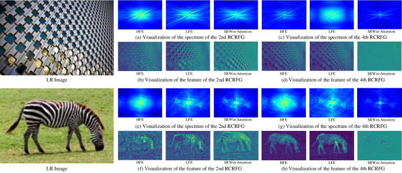
Figure 5: Visualization of HFERB and SRWAB. The LFE indicates the local feature extraction branch in HFERB, the HFE means the high-frequency enhancement branch in HFERB, and the SRWin-Attention represents the self-attention part in SRWAB.

Table 4: Complexity analysis compared to SwinIR.

Model	#Params. (K)	#FLOPs (G)	#GPU Mem. (M)	Ave. Time (ms)
SwinIR	897	32.2	141.2	72.0
CRAFT	753	26.1	79.5	42.8

5.4.3 Effectiveness of High-Frequency Prior

We conducted several experiments to investigate the effectiveness of high-frequency prior. Firstly, we swapped the input of $\boldsymbol{Q}$ and $\boldsymbol{K}$, $\boldsymbol{V}$ in HFB and treated the output of SRWAB as $\boldsymbol{Q}$ and the output of HFERB as $\boldsymbol{K}$, $\boldsymbol{V}$ to verify whether global features are dominant in restoration and high-frequency features only serve as a prior for refining the global representation. As shown in Table 3, compared to the original design, swapping the input leads to a significant drop in performance, with a 0.51dB decrease in PSNR. Furthermore, we also performed an experiment to formulate the model as a cascade structure to verify the effectiveness of the design introducing high-frequency priors. As shown in Table 3, the CRAFT_cascade structure resulted in a performance drop, with a 0.3dB decrease in PSNR compared to CRAFT. These results demonstrate the effectiveness of high-frequency priors in the CRAFT model.

5.4.4 Complexity analysis

We compared CRAFT with SwinIR in terms of complexity using an input size of $128\times 128$, as shown in Table 4. The analysis considered parameters, FLOPs, GPU memory consumption, and average inference time. GPU memory was measured using the official PyTorch function, and time cost was calculated based on 100 inference runs. Compared to SwinIR, CRAFT has fewer parameters and FLOPs, and requires less memory consumption and inference time. Additionally, we analyzed the complexity of our CRAFT framework and summarized the findings in Table 5. We observed that SRWAB contributes approximately 46% of the total complexity, while HFERB involves fewer convolution operations, resulting in reduced FLOPs. Furthermore, the HFB module’s channel-wise attention effectively reduces the computational burden.

Table 5: Complexity analysis of each block.

Model	CRAFT w/o HFERB	CRAFT w/o SRWAB	CRAFT w/o HFB	CRAFT
#Params. (K)	688	441	503	753
#FLOPs (G)	23.8	14.2	20.0	26.1

6 Conclusion

This paper investigates the impact of frequency on the performance of CNN and transformer structures in SISR and finds that transformer structures are more adept at capturing low-frequency information, but have limited capability to reconstruct high-frequency representations compared to CNN. To address this issue, we design a feature modulation transformer, named cross-refinement adaptive feature modulation transformer (CRAFT), which comprises three key components: the high-frequency enhancement residual block (HFERB), the shift rectangle window attention block (SRWAB), and the hybrid fusion block (HFB). The HFERB is designed to extract high-frequency features, while the SRWAB captures global representations. In the HFB, we treat the output of HFERB as a high-frequency prior and the output of SRWAB as key and value, and use inter-attention to refine the global representation. Experimental results demonstrate that CRAFT outperforms state-of-the-art methods by up to 0.29dB with relatively fewer parameters.

References

- [1] Eirikur Agustsson and Radu Timofte. Ntire 2017 challenge on single image super-resolution: Dataset and study. In Proceedings of the IEEE/CVF Conference on Computer Vision and Pattern Recognition Workshop (CVPRW), pages 126–135, 2017.
- [2] Namhyuk Ahn, Byungkon Kang, and Kyung Ah Sohn. Fast, accurate, and lightweight super-resolution with cascading residual network. In Proceedings of the European Conference on Computer Vision (ECCV), pages 256–272, 2018.
- [3] Marco Bevilacqua, Aline Roumy, Christine Guillemot, and Marie Line Alberi-Morel. Low-complexity single-image super-resolution based on nonnegative neighbor embedding. In Proceedings of the British Machine Vision Conference (BMVC), pages 1–10, 2012.
- [4] Hanting Chen, Yunhe Wang, Tianyu Guo, Chang Xu, Yiping Deng, Zhenhua Liu, Siwei Ma, Chunjing Xu, Chao Xu, and Wen Gao. Pre-trained image processing transformer. In Proceedings of the IEEE/CVF Conference on Computer Vision and Pattern Recognition (CVPR), pages 12299–12310, 2021.
- [5] Xiangyu Chen, Xintao Wang, Jiantao Zhou, Yu Qiao, and Chao Dong. Activating more pixels in image super-resolution transformer. In Proceedings of the IEEE/CVF Conference on Computer Vision and Pattern Recognition (CVPR), pages 22367–22377, 2023.
- [6] Zheng Chen, Yulun Zhang, Jinjin Gu, Yongbing Zhang, and Linghe Kong. Cross aggregation transformer for image restoration. In Proceedings of the Conference and Workshop on Neural Information Processing Systems (NeurIPS), 2022.
- [7] Chao Dong, Chen Change Loy, Kaiming He, and Xiaoou Tang. Image super-resolution using deep convolutional networks. IEEE Transactions on Pattern Analysis and Machine Intelligence, 38(2):295–307, 2016.
- [8] Faming Fang, Juncheng Li, and Tieyong Zeng. Soft-edge assisted network for single image super-resolution. IEEE Transactions on Image Processing, 29:4656–4668, 2020.
- [9] Guangwei Gao, Zhengxue Wang, Juncheng Li, Wenjie Li, Yi Yu, and Tieyong Zeng. Lightweight bimodal network for single-image super-resolution via symmetric cnn and recursive transformer. Proceedings of the International Joint Conference on Artificial Intelligence (IJCAI), 2022.
- [10] Hayit Greenspan. Super-resolution in medical imaging. The Computer Journal, 52(1):43–63, 2009.
- [11] Jinjin Gu and Chao Dong. Interpreting super-resolution networks with local attribution maps. In Proceedings of the IEEE/CVF Conference on Computer Vision and Pattern Recognition (CVPR), pages 9199–9208, 2021.
- [12] Jia-Bin Huang, Abhishek Singh, and Narendra Ahuja. Single image super-resolution from transformed self-exemplars. In Proceedings of the IEEE/CVF Conference on Computer Vision and Pattern Recognition (CVPR), pages 5197–5206, 2015.
- [13] Zheng Hui, Yunchu Yang, Xinbo Gao, and Xiumei Wang. Lightweight image super-resolution with information multi-distillation network. In Proceedings of the ACM International Conference on Multimedia (ACMMM), pages 2024–2032, 2019.
- [14] Sergey Ioffe and Christian Szegedy. Batch normalization: Accelerating deep network training by reducing internal covariate shift. In Proceedings of the International Conference on Machine Learning (ICML), pages 448–456, 2015.
- [15] Jiwon Kim, Jung Kwon Lee, and Kyoung Mu Lee. Accurate image super-resolution using very deep convolutional networks. In Proceedings of the IEEE/CVF Conference on Computer Vision and Pattern Recognition (CVPR), pages 1646–1654, 2016.
- [16] Christian Ledig, Lucas Theis, Ferenc Huszár, Jose Caballero, Andrew Cunningham, Alejandro Acosta, Andrew Aitken, Alykhan Tejani, Johannes Totz, Zehan Wang, et al. Photo-realistic single image super-resolution using a generative adversarial network. In Proceedings of the IEEE/CVF Conference on Computer Vision and Pattern Recognition (CVPR), pages 4681–4690, 2017.
- [17] Christian Ledig, Lucas Theis, Ferenc Huszár, Jose Caballero, Andrew Cunningham, Alejandro Acosta, Andrew Aitken, Alykhan Tejani, Johannes Totz, Zehan Wang, and Wenzhe Shi. Photo-realistic single image super-resolution using a generative adversarial network. In Proceedings of the IEEE/CVF Conference on Computer Vision and Pattern Recognition (CVPR), pages 105–114, 2017.
- [18] Wenbo Li, Xin Lu, Jiangbo Lu, Xiangyu Zhang, and Jiaya Jia. On efficient transformer and image pre-training for low-level vision. arXiv preprint arXiv:2112.10175, 2021.
- [19] Wenbo Li, Kun Zhou, Lu Qi, Nianjuan Jiang, Jiangbo Lu, and Jiaya Jia. Lapar: Linearly-assembled pixel-adaptive regression network for single image super-resolution and beyond. In Proceedings of the Conference and Workshop on Neural Information Processing Systems (NeurIPS), pages 1–13, 2020.
- [20] Zhen Li, Jinglei Yang, Zheng Liu, Xiaomin Yang, Gwanggil Jeon, and Wei Wu. Feedback network for image super-resolution. In Proceedings of the IEEE/CVF Conference on Computer Vision and Pattern Recognition (CVPR), pages 3867–3876, 2019.
- [21] Jingyun Liang, Jiezhang Cao, Guolei Sun, Kai Zhang, Luc Van Gool, and Radu Timofte. Swinir: Image restoration using swin transformer. In Proceedings of the IEEE/CVF Conference on Computer Vision Workshop (ICCVW), pages 1833–1844, 2021.
- [22] Jingyun Liang and Luc Van Gool. Flow-based Kernel Prior with Application to Blind Super-Resolution. In Proceedings of the IEEE/CVF Conference on Computer Vision and Pattern Recognition (CVPR), pages 10601–10610, 2021.
- [23] Bee Lim, Sanghyun Son, Heewon Kim, Seungjun Nah, and Kyoung Mu Lee. Enhanced deep residual networks for single image super-resolution. In Proceedings of the IEEE/CVF Conference on Computer Vision and Pattern Recognition Workshop (CVPRW), pages 1132–1140, 2017.
- [24] Ze Liu, Yutong Lin, Yue Cao, Han Hu, Yixuan Wei, Zheng Zhang, Stephen Lin, and Baining Guo. Swin transformer: Hierarchical vision transformer using shifted windows. In Proceedings of the IEEE/CVF Conference on Computer Vision (ICCV), pages 10012–10022, 2021.
- [25] Zhisheng Lu, Juncheng Li, Hong Liu, Chaoyan Huang, Linlin Zhang, and Tieyong Zeng. Transformer for single image super-resolution. In Proceedings of the IEEE/CVF Conference on Computer Vision and Pattern Recognition Workshop (CVPRW), pages 457–466, 2022.
- [26] Xiaotong Luo, Yuan Xie, Yulun Zhang, Yanyun Qu, Cuihua Li, and Yun Fu. Latticenet: Towards lightweight image super-resolution with lattice block. In Proceedings of the European Conference on Computer Vision (ECCV), pages 272–289, 2020.
- [27] David Martin, Charless Fowlkes, Doron Tal, and Jitendra Malik. A database of human segmented natural images and its application to evaluating segmentation algorithms and measuring ecological statistics. In Proceedings of the IEEE/CVF Conference on Computer Vision (ICCV), pages 416–423, 2001.
- [28] Yusuke Matsui, Kota Ito, Yuji Aramaki, Azuma Fujimoto, Toru Ogawa, Toshihiko Yamasaki, and Kiyoharu Aizawa. Sketch-based manga retrieval using manga109 dataset. Multimedia Tools and Applications, 76(20):21811–21838, 2017.
- [29] Yiqun Mei, Yuchen Fan, and Yuqian Zhou. Image Super-Resolution with Non-Local Sparse Attention. In Proceedings of the IEEE/CVF Conference on Computer Vision and Pattern Recognition (CVPR), pages 3517–3526, 2021.
- [30] Yiqun Mei, Yuchen Fan, Yuqian Zhou, Lichao Huang, Thomas S. Huang, and Humphrey Shi. Image super-resolution with cross-scale non-local attention and exhaustive self-exemplars mining. In Proceedings of the IEEE/CVF Conference on Computer Vision and Pattern Recognition (CVPR), 2020.
- [31] Sivaram Prasad Mudunuri and Soma Biswas. Low resolution face recognition across variations in pose and illumination. IEEE Transactions on Pattern Analysis and Machine Intelligence, 38(5):1034–1040, 2015.
- [32] Kamyar Nazeri, Harrish Thasarathan, and Mehran Ebrahimi. Edge-informed single image super-resolution. In Proceedings of the IEEE/CVF Conference on Computer Vision Workshop (ICCVW), pages 3275–3284, 2019.
- [33] Wenzhe Shi, Jose Caballero, Ferenc Huszár, Johannes Totz, Andrew Aitken, Rob Bishop, Daniel Rueckert, and Zehan Wang. Real-time single image and video super-resolution using an efficient sub-pixel convolutional neural network. In Proceedings of the IEEE/CVF Conference on Computer Vision and Pattern Recognition (CVPR), pages 1874–1883, 2016.
- [34] Bin Sun, Yulun Zhang, Songyao Jiang, and Yun Fu. Hybrid pixel-unshuffled network for lightweight image super-resolution. In Proceedings of the Association for the Advancement of Artificial Intelligence (AAAI), 2023.
- [35] Radu Timofte, Vincent De Smet, and Luc Van Gool. Anchored neighborhood regression for fast example-based super-resolution. In Proceedings of the IEEE/CVF Conference on Computer Vision (ICCV), pages 1920–1927, 2013.
- [36] Radu Timofte, Vincent De Smet, and Luc Van Gool. A+: Adjusted anchored neighborhood regression for fast super-resolution. In Proceedings of the Asian Conference on Computer Vision (ACCV), pages 111–126, 2014.
- [37] Tong Tong, Gen Li, Xiejie Liu, and Qinquan Gao. Image Super-Resolution Using Dense Skip Connections. In Proceedings of the IEEE/CVF Conference on Computer Vision (ICCV), pages 4809–4817, 2017.
- [38] Wenxiao Wang, Lu Yao, Long Chen, Binbin Lin, Deng Cai, Xiaofei He, and Wei Liu. Crossformer: A versatile vision transformer hinging on cross-scale attention. In Proceedings of the International Conference on Learning Representations (ICLR), 2022.
- [39] Zhou Wang, Alan C Bovik, Hamid R Sheikh, and Eero P Simoncelli. Image quality assessment: from error visibility to structural similarity. IEEE Transactions on Image Processing, 13(4):600–612, 2004.
- [40] Bin Xia, Yucheng Hang, Yapeng Tian, Wenming Yang, Qingmin Liao, and Jie Zhou. Efficient non-local contrastive attention for image super-resolution. In Proceedings of the Association for the Advancement of Artificial Intelligence (AAAI), pages 2759–2767, 2022.
- [41] Jianchao Yang, John Wright, Thomas S Huang, and Yi Ma. Image super-resolution via sparse representation. IEEE Transactions on Image Processing, 19(11):2861–2873, 2010.
- [42] Syed Waqas Zamir, Aditya Arora, Salman Khan, Munawar Hayat, Fahad Shahbaz Khan, and Ming-Hsuan Yang. Restormer: Efficient transformer for high-resolution image restoration. In Proceedings of the IEEE/CVF Conference on Computer Vision and Pattern Recognition (CVPR), pages 5718–5729, 2022.
- [43] Roman Zeyde, Michael Elad, and Matan Protter. On single image scale-up using sparse-representations. In International Conference on Curves and Surfaces (ICCS), pages 711–730, 2010.
- [44] Xindong Zhang, Hui Zeng, Shi Guo, and Lei Zhang. Efficient long-range attention network for image super-resolution. In Proceedings of the European Conference on Computer Vision (ECCV), 2022.
- [45] Xindong Zhang, Hui Zeng, and Lei Zhang. Edge-oriented convolution block for real-time super resolution on mobile devices. In Proceedings of the ACM International Conference on Multimedia (ACMMM), pages 4034–4043, 2021.
- [46] Yulun Zhang, Kunpeng Li, Kai Li, Lichen Wang, Bineng Zhong, and Yun Fu. Image super-resolution using very deep residual channel attention networks. In Proceedings of the European Conference on Computer Vision (ECCV), pages 294–310, 2018.
- [47] Zhengdong Zhang and Vivienne Sze. Fast: A framework to accelerate super-resolution processing on compressed videos. In Proceedings of the IEEE/CVF Conference on Computer Vision and Pattern Recognition (CVPR), pages 1015–1024, 2017.