Low temperature TBA and GHD for simple integrable QFT

Abstract

We derive the low temperature thermodynamic equations corrected by virtual processes for integrable QFT on large but finite size space circle. Obtained TBA’s are solved numerically for the sinh-Gordon model. We also derive corresponding Euler scale generalized hydrodynamics (GHD) equations.

Contents

1. 1 Introduction
2. 2 TBA with virtual excitations
   1. 2.1 Numerical solution of the TBA equations for the Sinh-Gordon model.
3. 3 Euler scale GHD
   1. 3.1 Dressing
   2. 3.2 Hydrodynamics
4. 4 Conclusions
5. A Some useful properties of the dressing operator

1 Introduction

Effective descriptions of many-body systems in terms of thermodynamics and hydrodynamics is arguably very successful approach to equilibrium and non-equilibrium phenomena. Its $(1+1)$ dimensional versions are useful playgrounds to test our understanding of extremely complicated physics present in higher dimensions. Thermodynamics of integrable models is well developed subject [1]. In recent years their hydrodynamical description has been successfully constructed and named GHD [2, 3]. The approach flourished in numerous developments [4, 5, 6, 7, 8, 9, 10] and extensions including effects of diffusion [11, 12] and dispersion[13]. GHD can be applied for quantum systems as well as classical gasses of solitons [14, 15]. Obtained results were confirmed by numerical simulations (see also [16]) as well as by experiments involving one dimensional cold atomic gases [17, 18, 19]. For detailed exposition of the subject we refer the reader to [20],[21] and [22].

Integrable QFT’s pose new problems due to virtual processes which come into play. It is known that at finite temperature virtual quasiparticles modify TBA equations [23, 24, 25, 26]. In consequence they also change GHD equations [27] but the proposed formulae are had to deal with: one need to solve generalized BE’s which is plagued with technical difficulties.

In this work we propose a generalization of the TBA equations that includes virtual processes of integrable relativistic QFT. The obtained formulae are valid at low temperatures. We shall also derive corresponding Euler scale GHD equations. The results depend heavily on relativistic invariance and the duality between finite but large temperature circle $R$ and the space circle $L$.

The paper is organized as follows. In Sec.2 we recall basic facts about virtual processes in integrable QFT with one type of quasiparticles. We shall take thermodynamic limit on the temperature circle obtaining set of four integral equations on densities and pseudoenergies which generalizes standard BYE and TBA equations. We solve numerically the system for the sinh-Gordon model for some values of free parameters of the theory. In the following section we derive the dressing operation which is an essential ingredient of the hydrodynamics. Next we write down explicit form of the GHD equations. We end with conclusions. The appendix A summarizes some properties of the dressing entering the discussed system.

2 TBA with virtual excitations

Our purpose is to describe thermodynamics of an integrable QFT defined on a circle of the large size $L$. In QFT the temperature is emulated by going to Euclidean time circle of the size $R$. Hence one deals with two circles $L$ and $R$ what gives possibility to interchange their role: $1/L$ enters some formulae as the dual temperature. We go to thermodynamic limit on both circles keeping $R$ and $L$ large but finite and introduce continuous densities for real (residing on $L$) and virtual (on $R$) quasiparticles.

In this paper we shall explicitly display formulae for theories with one type of quasiparticles for which the sinh-Gordon model [28, 29, 30] is a benchmark theory. The generalization to many quasiparticles case should be straightforward.

Our starting point is the standard TBA equation without virtual quasiparticles taken into account.

$${\boldsymbol{\epsilon}}_{0}(\theta)=E(\theta)-\frac{1}{R}\int\!\!{d\!\!\raisebox{6.02773pt}{\_}u}\,{}\Phi^{\prime}(\theta-u)\log(1+e^{-R{\boldsymbol{\epsilon}}_{0}(u)}),$$ (2.1)

where $\log S=i\Phi$ and $E(\theta)=m\cosh(\theta)$ for mass $m$ quasiparticles. Due to QFT phenomena virtual quasiparticles going around $R$ circle are present modifying (2.1) to

$${\boldsymbol{\epsilon}}(\theta)=E(\theta)+\frac{i}{R}\sum_{j}\Phi(\theta-\theta_{j}^{+})-\frac{1}{R}\int\!\!{d\!\!\raisebox{6.02773pt}{\_}u}\,{}\Phi^{\prime}(\theta-u)\log(1+e^{-R{\boldsymbol{\epsilon}}(u)})$$ (2.2)

Notice that virtual particles rapidities $\theta_{j}^{+}=\theta_{j}+\frac{i\pi}{2}$ reside in mirror channel according to standard nomenclature (see e.g. [31]). Their values are determined demanding:

$$R\,{\boldsymbol{\epsilon}}(\theta_{i}^{+})=i(2n_{i}+1)\pi,\quad n_{i}\in{\mathbb{Z}}$$ (2.3)

This yields BE corrected by the ground state contribution.

$$i(2n_{i}+1)\pi=R\,E(\theta^{+}_{i})+i\sum_{j}\Phi(\theta_{i}-\theta_{j})+i\pi-\int\!\!{d\!\!\raisebox{6.02773pt}{\_}u}\,{}\Phi^{\prime}(\theta^{+}_{i}-u)\log(1+e^{-R{\boldsymbol{\epsilon}}(u)})$$ (2.4)

Notice that the mirror energy respects: $E(\theta^{+}_{i})=i\,p(\theta_{i})$, where $p(\theta)$ is the relativistic momentum. The two sets of equations (2.2) and (2.4) determine pseudoenergy ${\boldsymbol{\epsilon}}$ and thus the occupation number $n=(1+e^{R{\boldsymbol{\epsilon}}})^{-1}$ of quasiparticles on $L$. The equations were analyzed to some extent in e.g. [26].

Going to thermodynamic limit for the virtual quasiparticles on the large circle $R$ we get

$${\boldsymbol{\epsilon}}(\theta)= E(\theta)+i\!\int\!du\ \Phi(\theta-u^{+})\tilde{{\boldsymbol{\rho}}}(u)-\frac{1}{R}\!\int\!\!{d\!\!\raisebox{6.02773pt}{\_}u}\,{}\Phi^{\prime}(\theta-u)\log(1+e^{-R{\boldsymbol{\epsilon}}(u)})$$ (2.5)

where $\tilde{{\boldsymbol{\rho}}}$ is the density of the virtual quasiparticles. Differentiating (2.4) over $\theta$ we get the modified BYE

$$2\pi i\tilde{{\boldsymbol{\rho}}}_{t}(\theta)=E^{\prime}(\theta^{+})+i\int\!du\,\Phi^{\prime}(\theta-u)\tilde{{\boldsymbol{\rho}}}(u)+\int\!\!{d\!\!\raisebox{6.02773pt}{\_}u}\,{}\Phi^{\prime}(\theta^{+}-u)n(u){\boldsymbol{\epsilon}}^{\prime}(\theta)$$ (2.6)

where we have used ${\boldsymbol{\epsilon}}^{\prime}(\theta^{+})=2\pi i\tilde{{\boldsymbol{\rho}}}_{t}(\theta)$ and $\tilde{{\boldsymbol{\rho}}}_{t}$ is density of the virtual states.

One sees that the above procedure yields two equations (2.5) and (2.6) on three unknown functions ${\boldsymbol{\epsilon}},\ \tilde{{\boldsymbol{\rho}}}_{t},\ \tilde{{\boldsymbol{\rho}}}$. Hence we need to supplement the system by an extra input. For large $L$ we can use dual picture of the situation in which we swap the role of $R$ and $L$ i.e. we can threat $R$ circle as space in which the density $\tilde{{\boldsymbol{\rho}}}$ is determined by the temperature $1/L$. The equations governing $\tilde{{\boldsymbol{\rho}}}$ are dual cousins of Eqs. (2.5) and (2.6). Notice that in the dual picture below we choose $\tilde{{\boldsymbol{\epsilon}}}^{\prime}(\theta^{-})=-2\pi i{\boldsymbol{\rho}}_{t}(\theta)$ instead of ${\boldsymbol{\epsilon}}^{\prime}(\theta^{+})=2\pi i\tilde{{\boldsymbol{\rho}}}_{t}(\theta)$ we had previously. The difference is irrelevant here due to $\Phi(\theta^{-}\!-u)=-\Phi(\theta^{+}\!-u)$ but we have found it useful for the construction of dressing to be discussed in the next section.

In this way we can write the complete set of equations on the unknowns: $\tilde{{\boldsymbol{\epsilon}}},\ \tilde{{\boldsymbol{\rho}}}_{t},\ {\boldsymbol{\epsilon}},\ {\boldsymbol{\rho}}_{t}$.

$${\boldsymbol{\epsilon}}(\theta)= E(\theta)+i\!\int\!{d\!\!\raisebox{6.02773pt}{\_}u}\,{}\ \Phi(\theta-u^{+})\tilde{n}(u)\tilde{{\boldsymbol{\rho}}}_{t}(u)-\frac{1}{R}\!\int\!\!{d\!\!\raisebox{6.02773pt}{\_}u}\,{}\Phi^{\prime}(\theta-u)\log(1+e^{-R{\boldsymbol{\epsilon}}(u)})$$ (2.7)

$$\tilde{{\boldsymbol{\rho}}}_{t}(\theta)= -i\,E^{\prime}(\theta^{+})+\!\int\!{d\!\!\raisebox{6.02773pt}{\_}u}\,{}\ \Phi^{\prime}(\theta-u)\tilde{n}(u)\tilde{{\boldsymbol{\rho}}}_{t}(u)+\frac{i}{R}\!\int\!\!{d\!\!\raisebox{6.02773pt}{\_}u}\,{}\Phi^{\prime\prime}(\theta^{+}-u)\log(1+e^{-R{\boldsymbol{\epsilon}}(u)})$$ (2.8)

$$\tilde{{\boldsymbol{\epsilon}}}(\theta)= E(\theta)+i\int\!{d\!\!\raisebox{6.02773pt}{\_}u}\,{}\ \Phi(\theta-u^{+})n(u){\boldsymbol{\rho}}_{t}(u)-\frac{1}{L}\!\int\!\!{d\!\!\raisebox{6.02773pt}{\_}u}\,{}\Phi^{\prime}(\theta-u)\log(1+e^{-L\tilde{{\boldsymbol{\epsilon}}}(u)})$$ (2.9)

$${\boldsymbol{\rho}}_{t}(\theta)= iE^{\prime}(\theta^{-})+\!\int\!{d\!\!\raisebox{6.02773pt}{\_}u}\,{}\ \Phi^{\prime}(\theta-u)n(u){\boldsymbol{\rho}}_{t}(u)-\frac{i}{L}\!\int\!\!{d\!\!\raisebox{6.02773pt}{\_}u}\,{}\Phi^{\prime\prime}(\theta^{-}-u)\log(1+e^{-L\tilde{{\boldsymbol{\epsilon}}}(u)}).$$ (2.10)

where $n(u)=(1+e^{R{\boldsymbol{\epsilon}}(u)})^{-1},\ \tilde{n}(u)=(1+e^{L\tilde{{\boldsymbol{\epsilon}}}(u)})^{-1}$ and we have also redefined $2\pi\tilde{{\boldsymbol{\rho}}}_{t}\rightarrow\;\!\tilde{{\boldsymbol{\rho}}}_{t}$, $2\pi{\boldsymbol{\rho}}_{t}\rightarrow\;\!{\boldsymbol{\rho}}_{t}$. In the limit $L\rightarrow\;\infty$ the occupation ratio $\tilde{n}\rightarrow\;0$ thus the virtual particles contribution to ${\boldsymbol{\epsilon}}$ vanishes and (2.7) and (2.10) become standard TBA and BYE, respectively. Notice that for the standard relativistic kinematics one can rescale ${\boldsymbol{\epsilon}}$’s and ${\boldsymbol{\rho}}$’s in such a way that the mass $m$ enters through products $R\,m,\ L\,m$ only.

2.1 Numerical solution of the TBA equations for the Sinh-Gordon model.

Here we shall display the numerical solutions to $n(\theta)$ from the TBA’s equations (2.7-2.10). We focus on the comparison between $n(\theta)$ and the solution $n_{0}(\theta)$ to the standard TBA equation (2.1) which discards virtual processes.

We do the calculations for the sinh-Gordon model which serves as a benchmark integrable QFT. It has just one type of quasiparticles [32, 33, 1, 34]. The two-particle scattering amplitude is

$$S(\theta) =\frac{\tanh\frac{1}{2}(\theta+i\pi x)}{\tanh\frac{1}{2}(\theta-i\pi x)}=\frac{\sinh(\theta)+ia}{\sinh(\theta)-ia}$$ (2.11)

with $a=\sin(\pi x)$. The scattering phase $\Phi=-i\,\log S(\theta)$ and its derivatives are:

$$\Phi(\theta^{+}) =-\Phi(\theta^{-})=\log(\frac{\cosh(\theta)-a}{\cosh(\theta)+a})$$ (2.12)

$$\varphi(\theta) =\Phi^{\prime}(\theta)=\frac{2a\,\cosh(\theta)}{\sinh^{2}(\theta)+a^{2}}$$ (2.13)

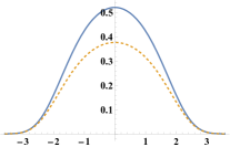
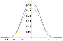
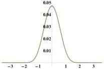
Figure 1: Plots of $n(\theta)$ (continues line) obtained from (2.7-2.10) vs. $n_{0}(\theta)$ (dashed line) from Eq.(2.1). The three plots correspond to $R=0.5,\ 1,\ 3$ going from left to right, while $a=0.5,L=3,m=1$. It is clear that the bigger $R$ the smaller are the virtual corrections: for the last case both plots nearly overlap.

3 Euler scale GHD

GHD is a very powerful tool devised to provide description of the macroscopic properties of integrable models [2, 3]. The relevant hydrodynamical quantities are densities and occupation numbers which, besides rapidity, depend on space-time coordinates: ${\boldsymbol{\rho}}(\theta,t,x),\ n(\theta,t,x)$, etc. Their dynamics is derived from (infinite) current conservation laws of the integrable models under consideration.

We start with brief description of technical steps which lead to Euler scale GHD. Let the complete set of functions (enumerated by $\lambda$) on the space of rapidities to be $h_{\lambda}(\theta)$. We define space-time densities of charges: $q_{\lambda}=\int d\theta\,{\boldsymbol{\rho}}\,h_{\lambda}=\int d\theta\,{\boldsymbol{\rho}}_{t}\,n\,h_{\lambda}$. The dressing of arbitrary function $g$ of rapidities is:

$$(g)^{\rm dr}(\theta)=g(\theta)+\int{d\!\!\raisebox{6.02773pt}{\_}u}\,{}\,\Phi^{\prime}(\theta-u)\,n(u)\,(g)^{\rm dr}(u)$$ (3.1)

or, in short $(g)^{\rm dr}=g+\varphi\star\,n(g)^{\rm dr}$, where $\varphi=\Phi^{\prime}$ and $\star$ denotes convolution. The dressing comes into play by BYE

$${\boldsymbol{\rho}}_{t}=p^{\prime}+\varphi\star n{\boldsymbol{\rho}}_{t}$$ (3.2)

which can be written as ${\boldsymbol{\rho}}_{t}=(p^{\prime})^{\rm dr}$. One can show that (see e.g. [20]), $q_{\lambda}=\int(p^{\prime})^{\rm dr}n\,h_{\lambda}=\int p^{\prime}n\,(h_{\lambda})^{\rm dr}$ . Applying the mirror transformation: $q_{\lambda}\rightarrow\;ij_{\lambda},\ p\rightarrow\;iE$ we obtain $j_{\lambda}=\int E^{\prime}n\,(h_{\lambda})^{\rm dr}=\int(E^{\prime})^{\rm dr}\,n\,h_{\lambda}$. From there and conservation laws of currents, $\partial_{t}q_{\lambda}+\partial_{x}j_{\lambda}=0$, one derives the leading order (Euler scale) GHD equations.

$$(p^{\prime})^{\rm dr}\partial_{t}n+(E^{\prime})^{\rm dr}\partial_{x}n=0$$ (3.3)

The above can be extended to include diffusive [11, 12] and dispersive terms [13].

3.1 Dressing

As we have seen dressing plays major role in construction of hydrodynamics. It expresses change of a quantity due to interaction with other particles in environment. It is clear that any change in the standard TBA and BYE equations leads to change of dressing (for (2.2) and (2.4) see [27]). Here we construct the new dressing operator reflecting properties of Eqs. (2.7-2.10).

Our starting point is Eq.(2.10) which we write as:

$${\boldsymbol{\rho}}_{t}= p^{\prime}+\varphi\star n{\boldsymbol{\rho}}_{t}+\varphi^{-}\star\tilde{n}{\boldsymbol{\rho}}_{t}^{+}$$ (3.4)

where $g^{\pm}(\theta)=g(\theta\pm i\pi/2)$. This indicates the expressions for charges.

$$q_{\lambda}=\int\hat{\boldsymbol{\rho}}_{t}\hat{n}\,\hat{h}_{\lambda}=\int({\boldsymbol{\rho}}_{t}nh_{\lambda}+{\boldsymbol{\rho}}_{t}^{+}\tilde{n}h_{\lambda}^{+})$$ (3.5)

We need $h_{\lambda}\in{\mathbb{R}}$ and $h_{\lambda}^{+}\in i{\mathbb{R}}$ due to ${\boldsymbol{\rho}}_{t}^{+}\in i{\mathbb{R}}$. The inhomogeneous linear relations (3.4) inspire our definition of the new dressing which should be something like ${\boldsymbol{\rho}}_{t}\sim(p^{\prime})^{\rm dr}$. Moreover we expect that it will respect an analogy of the algebraic relation $\int(p^{\prime})^{\rm dr}n\,h_{\lambda}=\int p^{\prime}n\,(h_{\lambda})^{\rm dr}$ used to derived ordinary GHD equations.

It is convenient to rewrite the dressing operator in the matrix form. Notice that from (3.4) we can write: ${\boldsymbol{\rho}}_{t}^{+}=(p^{\prime})^{+}+\varphi^{+}\star n{\boldsymbol{\rho}}_{t}+\varphi\star\tilde{n}{\boldsymbol{\rho}}_{t}^{+}$. Both can be put into

$$\hat{\boldsymbol{\rho}}_{t}= (\hat{p}^{\prime})^{\rm Dr}$$ (3.6)

where the new dressing is defined by

$$(\hat{g})^{\rm Dr}= \hat{g}+\hat{\varphi}\,\star\hat{n}\,(\hat{g})^{\rm Dr}$$ (3.7)

for

$$\hat{g}=\left(\!\!\begin{array}[]{c}g\\ g^{+}\end{array}\!\!\right),\;\hat{\varphi}=\begin{pmatrix}{\varphi}&{\varphi^{-}\!}\\ {\varphi^{+}\!}&{\varphi}\end{pmatrix},\;\hat{n}=\begin{pmatrix}{n}&0\\ 0&{\tilde{n}}\end{pmatrix}$$ (3.8)

where $g^{+}\in i{\mathbb{R}}$.

Similarly from (2.7) and (2.8) we get:

$$\hat{\boldsymbol{\epsilon}}^{\prime}= (\hat{E}^{\prime})^{\rm Dr}$$ (3.9)

It is worth to notice that both (3.9) and (3.6) involve the same dressing operation.

It is easy to show that the following holds (see also App.A):

$$\int(\hat{g})^{\rm Dr}\,\hat{n}\,\hat{h}=\int\hat{g}\,\hat{n}\,(\hat{h})^{\rm Dr}$$ (3.10)

what is all-important identity (see below Eq.(3.2)) leading to

$$q_{\lambda}=\int\hat{\boldsymbol{\rho}}_{t}\hat{n}\,\hat{h}_{\lambda}=\int\hat{p}^{\prime}\hat{n}\,(\hat{h}_{\lambda})^{\rm Dr}.$$ (3.11)

In fact, (3.10) can be treated as the defining identity of the dressing operation.

3.2 Hydrodynamics

Our construction of the hydrodynamics duplicates what has been described in the beginning of this section with some tweaking due to the new dressing we have just defined. Let $(\hat{g})^{\rm Dr}\equiv{\mathbf{Dr}}(\hat{g})$, where ${\mathbf{Dr}}=(1-\hat{\varphi}\star\hat{n})^{-1}$ in accordance with (3.7). Also ${\mathbf{{\bar{D}}r}}=(1-\hat{n}\hat{\varphi}\star)^{-1}$ respects $\hat{n}{\mathbf{Dr}}={\mathbf{{\bar{D}}r}}\,\hat{n}$ . Then for any space-time derivative $\partial$ we have: $\partial(\hat{n}\,(\hat{g})^{\rm Dr})={\mathbf{{\bar{D}}r}}\,\partial\hat{n}\,(\hat{g})^{\rm Dr}$ for any $\hat{g}(\theta)$. Using the above current conservation law reads: $\int\hat{h}_{\lambda}{\mathbf{{\bar{D}}r}}(\partial_{t}\hat{n}\,(\hat{p^{\prime}})^{\rm Dr}+\partial_{x}\hat{n}\,(\hat{E^{\prime}})^{\rm Dr})=0$ which must hold for all $\lambda$. The l.h.s. can be rewritten as: $\int(\hat{h}_{\lambda})^{\rm Dr}(\partial_{t}\hat{n}\,(\hat{p^{\prime}})^{\rm Dr}+\partial_{x}\hat{n}\,(\hat{E^{\prime}})^{\rm Dr})$ what is equivalent to: $\int{\hat{h}_{\lambda}}(\partial_{t}\hat{n}\,(\hat{p^{\prime}})^{\rm Dr}+\partial_{x}\hat{n}\,(\hat{E^{\prime}})^{\rm Dr})$. Thus finally we get the GHD equations in the form

$${\mathbf{{\bar{D}}r}}^{-1}{(\partial_{t}\hat{n}\,(\hat{p^{\prime}})^{\rm Dr}+\partial_{x}\hat{n}\,(\hat{E^{\prime}})^{\rm Dr})}=0.$$ (3.12)

We must stress that (3.12) intertwines dynamics of two occupation ratios: the physical ($n$) and virtual ($\tilde{n}$) quasi-particles.

The equations (3.12) are very involved. The reason is that the dressing ${\mathbf{Dr}}$ is non-local operator acting on the extended space of functions as in (3.8). The only way one can tackle the equations is through numerical calculations. We shall not analyze (3.12) here leaving the problem for the future work.

4 Conclusions

We have presented here the low temperature TBA and the GHD equations corrected by virtual processes for integrable QFT on large but finite size circle $L$. The results have been derived using duality between the space and the temperature circles. The approach can be applied whenever one can use thermodynamic limit on both circles. Obtained TBA’s have been solved numerically for the sinh-Gordon model and the results presented. We have also derived Euler scale GHD. The obtained formulae couple dynamics of two coupled fluids: the physical and virtual quasi-particles.

Equations proposed here need further studies. One could analyze virtual corrections by other methods e.g. following [27] and compare with our proposal. This would require the extensive numerical simulations. The obtained GHD equations have intriguing structure. It would interesting to explore their formal properties as well as analyze solutions e.g. small fluctuations numerically following the approach of [7]. The possible extensions of the equations include higher order terms of the hydrodynamical expansion [13]. We are planning to address these issues in future works.

Appendix A Some useful properties of the dressing operator

Here we describe some basic properties of the dressing operator and function spaces appearing in our formulation of GHD of the Section 3. The discussion is neither complete not rigorous and it is based on the finite dimensional analogs of the object we consider. This should be good enough for the numerical solutions of the obtained GHD equations (3.12).

Let the space of real analytic functions over rapidities be $F$ then we denote

$$\hat{F}=\{\hat{f}=(f,\,f^{+});f\in F\mbox{ and }f^{+}\in i\,F\},$$ (A.1)

where $f^{+}(\theta)=f(\theta+{i\pi}/2)$. We define the scalar product on the space $\hat{F}$.

$$\langle\hat{f}_{1}|\hat{f}_{2}\rangle=\int{{\hat{f}}_{1}}\hat{n}{\hat{f}}_{2}$$ (A.2)

which enters the expressions on charges (3.5). Dressing (3.7) is a symmetric operator in the above scalar product,

$$\langle(\mathfrak{f}_{1})^{\rm Dr}|\hat{f}_{2}\rangle=\langle\hat{f}_{1}|(\hat{f}_{2})^{\rm Dr}\rangle$$ (A.3)

as in Eq. (3.10). Moreover $({\hat{f}})^{\rm Dr}\in\hat{F}$. Let $(\hat{f})^{\rm Dr}\equiv{\mathbf{Dr}}\,{\hat{f}}$. ${\mathbf{Dr}}$ is invertible on $\hat{F}$. In consequence it can be diagonalized with non-zero eigenvalues $\lambda\neq 0$: ${\mathbf{Dr}}=\sum_{\lambda}\lambda|\hat{h}_{\lambda}\rangle\langle\hat{h}_{\lambda}|$, where we have used the bra-ket notation. Denote ${\mathfrak{f}}=(f,g)$ for arbitrary $f,g\in F$. Thus $\langle\hat{h}_{\lambda}|\mathfrak{f}\rangle=0$ for all $\lambda$ means that ${\mathbf{Dr}}\,{{\mathfrak{f}}}=0$ or equivalently ${\mathbf{Dr}}^{-1}\,{{\mathfrak{f}}}=0$. In the case of GHD we have $\mathfrak{f}=\hat{n}^{-1}(\partial_{t}\hat{n}\,(\hat{p^{\prime}})^{\rm Dr}+\partial_{x}\hat{n}\,(\hat{E^{\prime}})^{\rm Dr})$. But due to ${\mathbf{{\bar{D}}r}}\,\hat{n}=\hat{n}\,{\mathbf{Dr}}$ we also have $\hat{n}^{-1}{\mathbf{{\bar{D}}r}}^{-1}={\mathbf{Dr}}^{-1}\hat{n}^{-1}$. This directly leads to the GHD equations (3.12).

References

- [1] G. Mussardo, Statistical Field Theory, Oxford Graduate Texts, Oxford University Press (3, 2020).
- [2] O.A. Castro-Alvaredo, B. Doyon and T. Yoshimura, Emergent hydrodynamics in integrable quantum systems out of equilibrium, Phys. Rev. X 6, 041065 (2016) 6 (2016) 041065 [1605.07331].
- [3] B. Bertini, M. Collura, J. De Nardis and M. Fagotti, Transport in out-of-equilibrium xxz chains: Exact profiles of charges and currents, Phys. Rev. Lett. 117, 207201 (2016) 117 (2016) 207201 [1605.09790].
- [4] B. Doyon and T. Yoshimura, A note on generalized hydrodynamics: inhomogeneous fields and other concepts, SciPost Phys. 2, 014 (2017) 2 (2016) [1611.08225].
- [5] B. Doyon, Exact large-scale correlations in integrable systems out of equilibrium, SciPost Phys. 5, 054 (2018) 5 (2017) [1711.04568].
- [6] V.B. Bulchandani, R. Vasseur, C. Karrasch and J.E. Moore, Bethe-boltzmann hydrodynamics and spin transport in the xxz chain, Phys. Rev. B 97, 045407 (2018) 97 (2017) 045407 [1702.06146].
- [7] M. Panfil and J. Pawełczyk, Linearized regime of the generalized hydrodynamics with diffusion, SciPost Phys. Core 1, 002 (2019) 1 (2019) [1905.06257].
- [8] A.C. Cubero and M. Panfil, Generalized hydrodynamics regime from the thermodynamic bootstrap program, SciPost Phys. 8, 004 (2020) 8 (2019) [1909.08393].
- [9] J. De Nardis, B. Doyon, M. Medenjak and M. Panfil, Correlation functions and transport coefficients in generalised hydrodynamics, Journal of Statistical Mechanics: Theory and Experiment 2022 (2021) 014002 [2104.04462].
- [10] B. Doyon, G. Perfetto, T. Sasamoto and T. Yoshimura, Emergence of hydrodynamic spatial long-range correlations in nonequilibrium many-body systems, 2210.10009.
- [11] J. De Nardis, D. Bernard and B. Doyon, Hydrodynamic Diffusion in Integrable Systems, Physical Review Letters 121 (2018) 160603 [1807.02414].
- [12] J. De Nardis, D. Bernard and B. Doyon, Diffusion in generalized hydrodynamics and quasiparticle scattering, SciPost Physics 6 (2019) 049 [1812.00767].
- [13] J. De Nardis and B. Doyon, Hydrodynamic gauge fixing and higher order hydrodynamic expansion, J. Phys. A 56, 245001 (2023) 56 (2022) 245001 [2211.16555].
- [14] G.A. El, Soliton gas in integrable dispersive hydrodynamics, Journal of Statistical Mechanics: Theory and Experiment (2021) 114001 2021 (2021) 114001 [2104.05812].
- [15] T. Bonnemain, B. Doyon and G.A. El, Generalized hydrodynamics of the kdv soliton gas, Journal of Physics A: Mathematical and Theoretical 55 (2022) 374004 [2203.08551].
- [16] F. Møller, N. Besse, I.E. Mazets, H.-P. Stimming and N.J. Mauser, The dissipative generalized hydrodynamic equations and their numerical solution, 2212.12349.
- [17] M. Schemmer, I. Bouchoule, B. Doyon and J. Dubail, Generalized hydrodynamics on an atom chip, Phys. Rev. Lett. 122, 090601 (2019) 122 (2018) 090601 [1810.07170].
- [18] F. Møller, C. Li, I. Mazets, H.-P. Stimming, T. Zhou, Z. Zhu et al., Extension of the generalized hydrodynamics to the dimensional crossover regime, Phys. Rev. Lett. 126, 090602 (2021) 126 (2020) 090602 [2006.08577].
- [19] N. Malvania, Y. Zhang, Y. Le, J. Dubail, M. Rigol and D.S. Weiss, Generalized hydrodynamics in strongly interacting 1d bose gases, Science 373, 1129 (2021) 373 (2020) 1129 [2009.06651].
- [20] B. Doyon, Lecture notes on generalised hydrodynamics, SciPost Phys. Lect. Notes 18 (2020) (2019) [1912.08496].
- [21] V.B. Bulchandani, S. Gopalakrishnan and E. Ilievski, Superdiffusion in spin chains, J. Stat. Mech. (2021) 084001 2021 (2021) 084001 [2103.01976].
- [22] F.H.L. Essler, A short introduction to generalized hydrodynamics, Physica A,127572 (2022) (2023) 127572 [2306.17072].
- [23] M. Lüscher, Volume dependence of the energy spectrum in massive quantum field theories. 1. Stable particle states, Commun. Math. Phys. 104 (1986) 177.
- [24] M. Lüscher, Volume dependence of the energy spectrum in massive quantum field theories. 2. Scattering states, Commun. Math. Phys. 105 (1986) 153.
- [25] R.A. Janik, Review of AdS/CFT integrability, Chapter III.5: Lüscher corrections, Lett. Math. Phys. 99 (2010) 277 [1012.3994].
- [26] Z. Bajnok, J. Balog, M. Lájer and C. Wu, Field theoretical derivation of lüscher’s formula and calculation of finite volume form factors, Journal of High Energy Physics 2018 (2018) [1802.04021].
- [27] Z. Bajnok and I. Vona, Exact finite volume expectation values of conserved currents, Physics Letters B 805 (2019) 135446 [1911.08525].
- [28] A. Arinshtein, V. Fateyev and A. Zamolodchikov, Quantum s-matrix of the (1 + 1)-dimensional todd chain, Physics Letters B 87 (1979) 389.
- [29] A. Fring, G. Mussardo and P. Simonetti, Form factors for integrable lagrangian field theories, the sinh-gordon model, Nuclear Physics B 393 (1993) 413.
- [30] A. Koubek and G. Mussardo, On the operator content of the sinh-gordon model, Physics Letters B 311 (1993) 193.
- [31] S.J. van Tongeren, Introduction to the thermodynamic bethe ansatz, Journal of Physics A: Mathematical and Theoretical 49 (2016) 323005.
- [32] A. Zamolodchikov, On the thermodynamic bethe ansatz equation in the sinh-gordon model, Journal of Physics A: Mathematical and General 39 (2006) 12863 [hep-th/0005181].
- [33] J. Teschner, On the spectrum of the sinh-gordon model in finite volume, Nuclear Physics B 799 (2008) 403 [hep-th/0702214].
- [34] R. Konik, M. Lájer and G. Mussardo, Approaching the self-dual point of the sinh-gordon model, Journal of High Energy Physics 2021 (2020) [2007.00154].