Study of Jupiter’s Interior with Quadratic Monte Carlo Simulations

Abstract

We construct models for Jupiter’s interior that match the gravity data obtained by the Juno and Galileo spacecrafts. To generate ensembles of models, we introduce a novel quadratic Monte Carlo technique that is more efficient in confining fitness landscapes than affine invariant method that relies on linear stretch moves. We compare how long it takes the ensembles of walkers in both methods to travel to the most relevant parameter region. Once there, we compare the autocorrelation time and error bars of the two methods. For a ring potential and the 2d Rosenbrock function, we find that our quadratic Monte Carlo technique is significantly more efficient. Furthermore we modified the walk moves by adding a scaling factor. We provide the source code and examples so that this method can be applied elsewhere. Here we employ our method to generate five-layer models for Jupiter’s interior that include winds and a prominent dilute core, which allows us to match the planet’s even and odd gravity harmonics. We compare predictions from the different model ensembles and analyze how much an increase of the temperature at 1 bar and ad hoc change to the equation of state affects the inferred amount of heavy elements in atmosphere and in the planet overall.

1 Introduction

Since the Juno spacecraft inserted into orbit around Jupiter in 2016, it has provided us with unprecedented data for the planet’s magnetic field, gravity, and atmospheric abundances (Bolton et al., 2017). For this article, the improvement in the precision of the gravity measurements are particularly important. While, for example, the gravity harmonic $J_{4}$ had been determined to be $J_{4}\times 10^{6}=-587\pm 5$ with data from Pioneer and Voyager mission, it is now known with much higher precision, $J_{4}\times 10^{6}=‐586.6085\pm 0.0024$ (Durante et al., 2020). This has also led to a revision among the methods and assumptions that go into modelling the planet’s interior structure (Stevenson, 1982; Hubbard et al., 2002; Hubbard & Militzer, 2016; Wahl et al., 2017; Ni, 2018; Nettelmann et al., 2021) but the small error bars have made sampling the available space with interior models much more challenging. So here we generate ensembles of models for Jupiter’s interior with a novel Monte Carlo (MC) method. We employ a number of different model assumption starting from our reference ensemble of five layer models (Militzer et al., 2022) that invoke a prominent dilute core that reach out to $\sim$60% of the planet’s radius as well as contributions from winds that we derived by solving thermal wind equation (Kaspi, 2013) in an oblate geometry. Interior and wind parameters are optimized simultaneously, which enabled us to improve upon solutions by Wahl et al. (2017) and match the Juno gravity measurements exactly.

In our second ensemble we raise the 1 bar temperature to 170 K from our reference value of 166.1 K that was determined in situ by the Galileo entry probe by matching the temperature-pressure data points to a dry adiabat (Seiff et al., 1998). While this fit has a very small temperature uncertainty, it is not certain to what degree this measurement represents the planet’s global average because the entry probe fell into a 5 $\mu$m hot spot and thus local weather effects may have played a role. However, one should not expect deviations to be too large because radio occultation measurements by the Voyager spacecrafts determined the 1 bar temperature to be 165 $\pm$ 5 K (Lindal et al., 1981). These remote observations very recently re-analyzed by Gupta et al. (2022) who determined higher temperatures of 167$\pm$4 and 170$\pm$4 K for latitudes of 6^∘S and 12^∘N respectively. The temperature increase was primarily caused by including the chemical species CH₄, Ne, Ar, and PH₃ when the molecular weight of atmosphere was calculated while the original value of 165 $\pm$ 5 K was derived by assuming a hydrogen-helium atmosphere that is free of heavier species.

Given these uncertainties, we constructed an ensemble with $T_{\rm 1bar}=170\,$K here while other authors have consider similar or even higher values. Kerley (2004) constructed models with $T_{\rm 1bar}$= 169 K. Recently, Nettelmann et al. (2021) constructed models with $T_{\rm 1bar}$= 175 and 180 K. Miguel et al. (2022) made the 1 bar temperature a free Monte Carlo parameter and obtained the best match to the Juno data while using 1 bar temperatures between 177 and 188 K. Such a temperature increase may be very appealing because it increase the entropy of the isentrope and there lowers the density everywhere in the planet. This makes it easier to match the Juno measurements of the gravity coefficients $J_{4}$ and $J_{6}$ and more importantly introduces additional flexibilities into the model to move heavy elements from one layer to another. Eventually, however, the temperature will be so high that the isentrope no longer intersect the immiscibility region of hydrogen-helium mixtures (Morales et al., 2013), which provides the basis for the helium rain argument that explains why the Galileo entry probe measured Jupiter’s atmospheric helium abundance [$Y/(X+Y)=0.238\pm 0.005$ von Zahn et al. (1998)] to be depleted compared to the protosolar value of $Y_{0}/(X_{0}+Y_{0})=0.2777$ (Lodders, 2010). Based on the semi-analytical equation of state (EOS) by Saumon et al. (1995) and ab initio EOS by Militzer & Hubbard (2013), we estimate a value for 1 bar temperature of 180 K for helium rain to have started. However, we derived this value exclusively with theoretical methods while the first experimental work, that indirectly inferred the conditions of H-He phase separation at megabar pressures, placed the onset for this process at much higher temperatures (Brygoo et al., 2021).

In our third ensemble, we modify the EOS that we derived with ab initio computer simulations and lowered the density by 3% (Militzer & Hubbard, 2023) in the pressure interval from 10 to 100 GPa where Militzer et al. (2022) found the models to be particularly sensitive. Such ad hoc EOS corrections have been introduced many times in the past when the modeling assumptions by themselves did not yield a good match to the observations. Nettelmann et al. (2021) lowered the density from 30–200 GPa because without a dilute core nor winds, the Juno gravity data could not be reproduced. There is no reason to assume that the ab initio EOS calculations are accurate to 1% level that is typically assumed to required to model giant planet interiors accurately. One reason for this level of accuracy is that one aims to estimate the abundance of heavy elements relative to the protosolar value of 1.53% (Lodders, 2010).

To the gravity coefficients $J_{4}$ and $J_{6}$, we assume in all three ensembles that Jupiter’s core has been substantially diluted with hydrogen and helium. The heavily elements, that were essential to trigger Jupiter’s formation, make up only $\sim$18% by mass. Core dilution is plausible because ab initio computer simulations have shown that all typical core materials such as water, silicates and iron are soluble in metallic hydrogen at megabar pressures (Wilson & Militzer, 2012a, b; Wahl et al., 2013; Gonzalez-Cataldo et al., 2014). It is less clear whether the convection in Jupiter’s interior is sufficiently strong to bring up the heavy elements against the forces of gravity (Guillot et al., 2004). Moll et al. (2017), Müller et al. (2020), and Helled et al. (2022) studied the interior convection and the evolution of a primordial, compact core that was originally compose to 100% of heavy elements. Liu et al. (2019) studied whether Jupiter core could be diluted by a giant impact. It is conceivable that a small compact core exists in inside the dilute core but it could not be very massive because that would take away from the dilute core effect that enabled us to match $J_{4}$ and $J_{6}$. Militzer et al. (2022) placed an upper limit of 3 Earth masses (1% of Jupiter’s mass) on the compact core.

Various papers have investigated the effects that different EOSs have on the inferred properties of Jupiter (Saumon & Guillot, 2004; Miguel et al., 2016). Because there are uncertainties in the EOS, we constructed ensembles of models for which we have lower density in a pressure window from $P^{*}$ to $10\times P^{*}$ and then moved across the entire pressure range of Jupiter’s interior in order to determine on which interval the model predictions depends most sensitively. It was our goal to provide some guidance to future experimental and theoretical work on where to expect the biggest impact for giant planet physics.

We analyze how such EOS change affect the heavy element abundance that is inferred for the planet’s outer envelope. Constructing models with subsolar or even with a “negative” abundance of heavy elements has enabled previous works to match or nearly match the Juno measurements for $J_{4}$ and $J_{6}$ without invoking a dilute core or winds (Hubbard & Militzer, 2016). On the other hand if one makes the assumptions that Jupiter form via core accretion from a well mixed protosolar nebula, the heavy elements in its atmosphere should occur in at least solar abundances. The small number of measurements and remote observations that exist for the atmospheric composition of giant planets have been reviewed in Atreya et al. (2019). With the exception of neon, the Galileo entry probe measured the nobel gases to be three-fold enriched compared to solar. Carbon has found to to be 4$\times$ solar in Jupiter and 9$\times$ solar in Saturn. If the same enrichment applied to oxygen and if these measurements were representative of the Jupiter’s entire envelope, it would pose a major challenge to all modeling activities because most models that match Juno’s $J_{4}$ and $J_{6}$ only yield heavy elements abundance in approximately solar proportions. (The same challenge exists for Saturn, for which typical models (Militzer et al., 2019) predict up to 4$\times$ solar abundance for heavy elements, which is well below the nine-fold solar measurements for carbon.)

The biggest unknown, however, is the concentration of oxygen, the most abundant element besides hydrogen and helium. Its abundance informs us about water which crucial for understanding where and how Jupiter formed (Helled & Lunine, 2014). The Galileo entry probe measured oxygen to be half solar bringing the total heavy element mass fraction to 1.7% before the probe stopped functioning at a pressure of 22 bar. More recently Li et al. (2020) used Juno’s microwave measurements to infer an oxygen abundance between one and five times solar. A more precise determination was not possible because the water signal is small compared to that of ammonia and its radiative properties at relevant conditions are not sufficiently well understood, which provides us with ample motivation to analyze the amount of heavy element that emerge from our model assumptions.

In this article, we construct three ensembles of model of Jupiter’s interior by introducing a novel Markov chain Monte Carlo methods the relies on quadratic rather affine (or linear) moves that are employed by Goodman & Weare (2010). We show that our method is more efficient in confining geometries that are difficult to sample with linear moves. Since its inception, the affine invariance sampling method has gained a remarkable level of acceptance in various fields of science including astronomy and astrophysics where one often needs to determine posterior distributions of model parameters that are compatible with observational data that carry uncertainties. For example, the affine sampling method has been employed to detect stellar companions in radial velocity catalogues (Price-Whelan et al., 2018), to study the relationship between dust disks and their host stars (Andrews et al., 2013), to examine the first observations of the Gemini Planet Imager (Macintosh et al., 2014), to analyze photometry data of Kepler’s K2 phase (Vanderburg & Johnson, 2014), to study the mass distribution in our Milky Way galaxy (McMillan, 2017), to identify satellites of the Magellanic Clouds (Koposov et al., 2015), to analyze gravitational-wave observations of a binary neutron star merger (De et al., 2018), to constrain Hubble constant with data of the cosmic microwave background (Bernal et al., 2016), or to characterize the properties of M-dwarf stars (Mann et al., 2015) to name a few applications. On the other hand, Huijser et al. (2022) demonstrated that the affine invariant method exhibits undesirable properties when the multivariate Rosenbrock density is sampled for more than 50 dimensions.

Goodman & Weare (2010) chose to perform their Markov chain Monte Carlo simulations with an entire ensemble of walkers (or states) rather than propagating just a single walker. The distribution of walkers in the ensemble helps one to propose favorable moves that have an increased chance of being accepted without the need for a detailed investigation of the local fitness landscape as the traditional Metropolis-Hastings Monte Carlo method requires. Many extensions of the Metropolis-Hastings approach have been advanced (Andrieu & Thoms, 2008). For example, Haario et al. (2001) use the entire accumulated history along the Monte Carlo chain of states to adjust the shape of the Gaussian proposal function.

Ensembles of walkers have been employed long before Goodman & Weare (2010) in various types of Monte Carlo methods that were designed for specific applications. In the fields of condensed matter physics and quantum chemistry, ensembles of walkers are employed in variational Monte Carlo (VMC) calculations (Martin et al., 2016) that optimize certain wavefunction parameters with the goal of minimizing the average energy or its variance (Foulkes et al., 2001). Ensembles are used to vectorize or parallelize the VMC calculations. They are also employed generate the initial set of configurations for the walkers in diffusion Monte Carlo (DMC) simulations. In DMC calculations, one samples the groundstate wave function by combining diffusive moves with birth and death processes. An ensemble of walkers is needed to estimate the average local energy so that the birth and death rates lead to a stable population size. Walkers with a low energy are favored and thus more likely to be selected to spawn additional walkers. Walkers in areas of high energy are likely to died out.

The birth and death concepts in DMC have a number of features in common with genetic algorithms that employ a population of individuals (similar to an ensemble of walkers). The best individuals are selected and modified with a variety of approaches to generate the next generation of individuals (Schwefel, 1981; Militzer et al., 1998). The population is needed to establish a fitness scale that enables one to make informed decisions which individuals should be selected for procreation. This scale will change over time as the population migrates towards for favorable regions in the parameter space. This also occurs in DMC calculations as the walker population migrates towards regions of low energy, the average energy in the population stabilizes, and the local energy approaches the ground state energy of the system.

Ensembles of individuals/walkers are not only employed in genetic algorithm but are used in many different stochastic optimization techniques. These methods have primarily been designed for the goal of finding the best state in a complex fitness landscape, or a state that is very close to it, rather than sampling a well-defined statistical distribution function as Monte Carlo method do. Therefore these optimization are much more flexible than Monte Carlo algorithms that typically need to satisfy the detailed balance relation for every move (Kalos & Whitlock, 1986).

The particle swarm optimization method (J. Kennedy & Eberhart, 1997, 2001) employs an ensemble (or swarm) of walkers and successively updates their locations according to a set of velocities. The velocities are updated stochastically using an inertial term and drift terms favor migration towards the best individual in the population and/or towards the global best ever generated.

Furthermore, the downhill simplex method (Press et al., 2001) employs an ensemble of $N+1$ walkers in $N$ dimensions. The optimization algorithm successively moves the walker with the highest or second highest energy in the ensemble in the direction of the center of mass of the other walkers. The ensemble of walkers thereby migrates step by step to more favorable locations in the fitness landscape without the need to ever compute a derivative of the fitness function, which makes this algorithm very appealing in situations where the fitness function is complex and its derivates cannot be derive with reasonable effort.

In general, efficient Monte Carlo methods are required to have two properties. They need to migrate efficiently in parameter space towards the most favorable region. The migration (or convergence) rate is typically measured in Monte Carlo time (or steps). Once the favorable region has been reached and average properties among walkers have stabilized, the Monte Carlo method needs to efficient sample the relevant parameter space. The efficiency of the algorithm is typically measured in terms of the autocorrelation time or the size of the error bars. While in typical applications, algorithms that have fast migration rates also have a short autocorrelation time, there is no guarantee that both are linked because the properties of fitness landscape may differ substantially between the initial and the most favorable regions of the parameter space. For this reason, we measure the migration rate and autocorrelation time separately when we evaluate the performance of the quadratic Monte Carlo method that we introduce in this article.

This article is organized as follows. In section 2, we introduce our quadratic Monte Carlo technique and compare it with the affine invariance method. We also describe how we construct models for Jupiter’s interior. In section 3 we present four sets of results. Frist we compare how the two methods perform for a ring potential problem and for the Rosenbrock density, then construct different ensembles of Jupiter’s interior, and finally study the consequences of various corrections to the assumed EOS for the inferred heavy element abundances in Jupiter’s outer molecular layer. In section 4, we conclude. In the appendix, we show that our quadratic Monte Carlo satisfy the condition of detailed balance.

2 Methods

2.1 Quadratic Moves

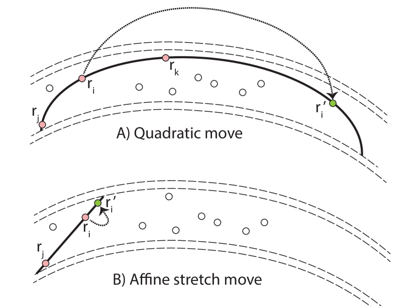
Figure 1: Illustration of quadratic and affine stretch moves in a confining channel that is represented by the dashed lines. The circles indicate the locations of walkers in the ensemble. For the quadratic move, two helper points $\vec{r}_{j}$ and $\vec{r}_{k}$ are employed to sample a new location for walker $i$. Conversely, for the stretch move, only one additional point $\vec{r}_{j}$ is used and walker $i$ may thus not travel as far in a single step in a curved channel.

We divide our Markov chain MC calculations into $N_{b}$ blocks, each consisting of $N_{S}$ steps. During every step, we attempt to move each of $N_{W}$ walkers in the ensemble once. A quadratic MC move proceeds as follows. In addition to the moving walker $i$, we select two other walkers $j$ and $k$ from the ensemble at random. Then we perform a quadratic Lagrange interpolation/extrapolation to sample new parameters, $\vec{r}_{i}^{\prime}$, for walker $i$,

$$\vec{r}_{i}^{\prime}=w_{i}\vec{r}_{i}+w_{j}\vec{r}_{j}+w_{k}\vec{r}_{k}$$ (1)

The interpolation weights $w$ are chosen from,

$$w_{i} = L(t^{\prime}_{i}\,;\,t_{i},t_{j},t_{k}),$$ (2)

$$w_{j} = L(t^{\prime}_{i}\,;\,t_{j},t_{k},t_{i}),$$ (3)

$$w_{k} = L(t^{\prime}_{i}\,;\,t_{k},t_{i},t_{j}),$$ (4)

$$L(x\,;\,x_{0},x_{1},x_{2}) \equiv \frac{x-x_{1}}{x_{0}-x_{1}}\frac{x-x_{2}}{x_{0}-x_{2}}$$ (5)

The function $L$ is the typical Lagrange weighting function that guarantees a proper quadratic interpolation so that $\vec{r}_{i}^{\prime}=\vec{r}_{i}$ if $t_{i}^{\prime}=t_{i}$; $\vec{r}_{i}^{\prime}=\vec{r}_{j}$ if $t_{i}^{\prime}=t_{j}$; and $\vec{r}_{i}^{\prime}=\vec{r}_{k}$ if $t_{i}^{\prime}=t_{k}$. We always set $t_{j}=-1$ and $t_{k}=+1$ to introduce a scale into the parameter space, $t$. To satisfy the detailed balance condition, $T(\vec{r}_{i}\to\vec{r}_{i}^{\prime})=T(\vec{r}_{i}^{\prime}\to\vec{r}_{i})$, it is key that we sample the parameters $t_{i}$ and $t_{i}^{\prime}$ from the same distribution $\mathcal{P}(t)$. (We do not set $t_{i}=0$ but sample it in the same way as $t_{i}^{\prime}$.) The acceptance probability then becomes,

$$A(\vec{r}_{i}\to\vec{r}_{i}^{\prime})=\min\left[1,\frac{\pi(\vec{r}_{i}^{\prime})}{\pi(\vec{r}_{i})}\,\left|w_{i}\right|^{N}\right]\;.$$ (6)

The factor $\left|w_{i}\right|^{N}$ is needed because we sample the one-dimensional $t$ space but then switch to the $N$-dimensional parameter space, $\vec{r}$. It plays the same role as the $\lambda^{\alpha}$ factor of the affine transformation that we discuss below. In appendix A, we derive this factor rigorously from the generalized detailed balance equation by Green & Mira (2001).

For the sampling distribution, $\mathcal{P}(t)$, one has a bit of a choice. Our applications have shown that the precise shape is not important but the width the distribution affects the MC efficiency in the usual way. If one tries to make too large steps in parameter space, too many moves are rejected. If the steps are chosen too small, most moves will be accepted but the resulting states are highly correlated and the parameter space is not explored efficiently either. So we introduce a constant scaling parameter, $a$, that controls the width of our sampling functions $\mathcal{P}(t)$. Besides the number of walkers, $N_{W}$, this is the only parameter a user of our quadratic MC method needs to adjust. $a=1.5$ is a perfectly fine choice. Only if a lot of computer time is to be invested, one may want to compare the MC efficiency for various $a$ values as we do in the next section. For the sampling functions, $\mathcal{P}(t)$, we propose two options:
a) We sample $t_{i}$ and $t^{\prime}_{i}$, uniformly from the interval $[-a,+a]$ or
b) we draw them independently from a Gaussian distribution that we center around zero and set the standard deviation equal to $a$.

In Fig. 1, we given an illustration for why quadratic moves tend to perform well in confined geometries. The move of walker $i$ is guided by the positions of walkers $j$ and $k$, which both reside in the narrow channel. Large moves become possible as long as the channel curvature does not change too rapidly. If it does, one may reduce the parameter $a$. For $t_{i}$ values that are sampled from the interval $[-a,+a]$, the parameter $a$ controls the probability that we choose the new walker location, $\vec{r}_{i}^{\prime}$, by interpolating between $\vec{r}_{j}$ and $\vec{r}_{k}$ ($|t_{i}^{\prime}|\leq 1$) or by extrapolating from these two points ($|t_{i}^{\prime}|>1$).

In Fig. 1, we also illustrate the affine stretch moves (Goodman & Weare, 2010) for comparison. To sample the new location for walker $i$, the position of only one other walker, $j$, is employed to construct this linear transformation,

$$\vec{r}_{i}^{\prime}=\vec{r}_{j}+\lambda(\vec{r}_{i}-\vec{r}_{j})$$ (7)

To make such moves reversible, the stretch factor, $\lambda$, must be sampled from the interval $\left[\frac{1}{a},a\right]$. For the sampling function, $T(\lambda)$, one has a bit of choice. Goodman & Weare (2010) followed Christen (2007) when they chose a function that satisfies,

$$T_{1}(\lambda)\; = \;\frac{1}{\lambda}\;T_{1}(\frac{1}{\lambda})$$ (8)

$$T_{1}(\lambda)\; \propto \;\frac{1}{\sqrt{\lambda}}\;\rm{if}\;\lambda\in\left[\frac{1}{a},a\right]\;\;.$$ (9)

This function can be sampled by choosing a random number, $\eta$, uniformly in [0,1] and transforming it according to,

$$\lambda=\frac{(\eta-d)^{2}}{d^{2}a}\;\;\rm{with}\;\;d=\frac{1}{1-a}$$ (10)

Alternatively, we can sample $\lambda$ in Eq. 7 uniformly from the interval $\left[\frac{1}{a},a\right]$,

$$T_{2}(\lambda)=\frac{a}{a^{2}-1}=\rm{constant~{}if~{}}\lambda\,\in\,\left[\frac{1}{a},a\right]{\rm and~{}T_{2}(\lambda)=0~{}elsewhere.}$$ (11)

For both sampling functions, a factor, $\lambda^{\alpha}=\frac{\left|\vec{r}_{i}^{\prime}-\vec{r}_{j}\right|^{\alpha}}{\left|\vec{r}_{i}-\vec{r}_{j}\right|^{\alpha}}$, must be introduced to the acceptance probability,

$$A(\vec{r}_{i}\to\vec{r}_{i}^{\prime})=\min\left[1,\frac{\pi(\vec{r}_{i}^{\prime})}{\pi(\vec{r}_{i})}\lambda^{\alpha}\right]\;.$$ (12)

For the uniform distribution, $T_{2}(\lambda)$, one sets $\alpha=N-2$ while one sets $\alpha=N-1$ for $T_{1}(\lambda)$. Both factors are caused by the fact that in $N$ dimensions, the area of a sphere around the anchor point $\vec{r}_{j}$ scales with $\left|\vec{r}_{i}-\vec{r}_{j}\right|^{N-1}$. The uniform distribution, $T_{2}(\lambda)$ already stretches the interval of $a$ values automatically and therefore $\alpha$ is set to $N-2$ rather than $N-1$. A derivation for these factors is provided in appendix A.

As a first, very basic test whether any of these methods works correctly, we applied them to sample the Boltzmann distribution,

$$\pi(\vec{r})\propto\exp\left\{-\frac{V(\vec{r})}{k_{B}T}\right\}$$ (13)

for a harmonic potential in $N$ dimensions, $V(\vec{r})=\sum_{d=1}^{N}r_{d}^{2}$, in order to verify that the resulting average potential energy, $\left<V\right>$, agrees with the exact value of $NT/2$ within error bars. (We set the Boltzmann constant, $k_{B}$, to 1 throughout this paper.) This is also a reasonable first test whether the factors in the acceptance ratios in Eqs. 6 and 12 are set correctly. As a second test in section 3.1, we compared the average potential energy that we obtained with the affine and our quadratic MC method for a computationally more challenging ring potential.

2.2 Modified Walk Moves

Goodman & Weare (2010) also introduced an alternate sampling method: walk moves. To move walker $k$ from $\vec{r}_{k}$ to $\vec{r}_{k}^{\prime}=\vec{r}_{k}+W$, one chooses at random a subset, $S$, of $N_{S}$ guiding walkers. $k$ is excluded from $S$ so that the positions in the subset are independent of $\vec{r}_{k}$. The subset size, $N_{S}$, is a free parameter that one needs to choose within $2\leq N_{S}<N_{W}$. We typically keep $N_{S}$ constant for an entire MC chain but we have also performed calculations with a flexible subset size, for which we selected walkers for the subset according to a specified probability, $p_{S}$, but we found no advantages in using a flexible $N_{S}$ number over a fixed value.

We follow Goodman & Weare (2010) in computing the average location all walkers in the subset,

$$\left<\vec{r}\right>=\frac{1}{N_{S}}\sum_{j\in S}\vec{r}_{j}\quad.$$ (14)

but we then modify their formula for computing the step size, $W$, by introduding a scaling factor $a$:

$$W=a\sum_{j\in S}Z_{j}\left(\vec{r}_{j}-\left<\vec{r}\right>\right)\quad.$$ (15)

$Z_{j}$ are univariate standard normal random numbers. By setting $a=1$, one obtains the original walk moves, for which the covariance of the step size, $W$, is the same as the covariance of subset $S$. However, the new scaling parameter, $a$, enables us to make smaller (or larger) steps in situations where the covariance of the instantaneous walker distribution is a not an optimal representation of local structure of the sampling function. We will show later that the scaling factor $a$ enables us to significantly improve the sampling efficiency of the Rosenbrock function and for the ring potential in high dimensions.

2.3 Equation of State

The EOS of hydrogen-helium mixtures plays a crucial role in the modeling Jupiter’s interior structure because both gases make up the bulk of the planet. We derive he EOS by combining the Saumon et al. (1995) predictions at low pressure and with results from ab initio computer simulations at high pressure (P $\geq$ 5 GPa) (Militzer & Hubbard, 2013). For a given composition and entropy, both EOSs provide a $\rho(P)$ relationship. One can gradually switch from one to the other as function of pressure. Still there are two primary sources of uncertainty to consider:

(1) First, current ab initio calculations are based on the density functional theory and employed on the PBE functional (Perdew et al., 1996) while other choices are possible. Currently we lack experimental data to determine how accurately any of the existing functionals (Clay et al., 2016) characterize liquid hydrogen at megabar pressures. X-ray diffraction experiments of solid materials at room temperature have shown that the PBE functional underestimates the density of materials by a few % while the earlier local density approximation, that was constructed from results by Ceperley & Alder (1980), overestimates the density of solids. However, simulations based on the PBE functional are in very good agreement with the shock wave measurements (see Knudson & Desjarlais (2017) and Militzer et al. (2016)) that measured the density of deuterium at megabar pressure more accurately than previously possible. Still accurate density measurements of liquids remain a challenged because X-ray diffraction measurements cannot be applied. On the other hand, quantum Monte Carlo calculation (Mazzola et al., 2018) have predicted hydrogen to be more dense than the PBE predictions. However, a higher-than-PBE density relationship would make the modeling of Jupiter’s interior more difficult and likely lead to subsolar heavy element abundance in the other envelope, as we will discuss in the results section of this manuscript.

(2) The second EOS uncertainty arise from the temperature profile of the isentropes. Locally this is characterized by the Grüneisen parameter, $\gamma=-\left.\frac{\partial\ln T}{\partial\ln V}\right|_{S}=T\left.\frac{\partial P}{\partial T}\right|_{V}/\left.\frac{\partial E}{\partial T}\right|_{V}$ (Militzer & Hubbard, 2007). Globally, one can state that the temperature at 1 bar defines an entropy value that determines $P$-$T$ relationship for the entire thickness of layer in the planet as long as it is homogeneous and convective. Different predictions from local and global approaches have led to very different predictions how hot Jupiter’s interior is (Militzer et al., 2008; Nettelmann et al., 2008). With the global approach, one determine the absolute entropy for a grid of $\rho$-$T$ point with the thermodynamic integration method (Morales et al., 2009; Militzer, 2013) and then find the isentrope through interpolation. We favor this approach (Militzer & Hubbard, 2009) because every $S(\rho,T)$ point is independent. So if one particular calculation were inaccurate, it would not affect the results elsewhere. With the local approach, one needs a very dense grid EOS points to numerically compute the derivatives that are needed trace an isentrope by computing $\gamma$ at every step. A second and important reason for the disagreement on Jupiter’s interior temperature profile was that the local approach requires a reliably starting point for the isentrope and ab initio simulations do not work at 1 bar because the density is too low.

2.4 Modeling Jupiter’s Interior

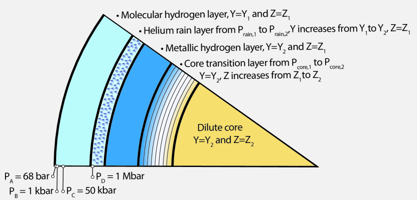
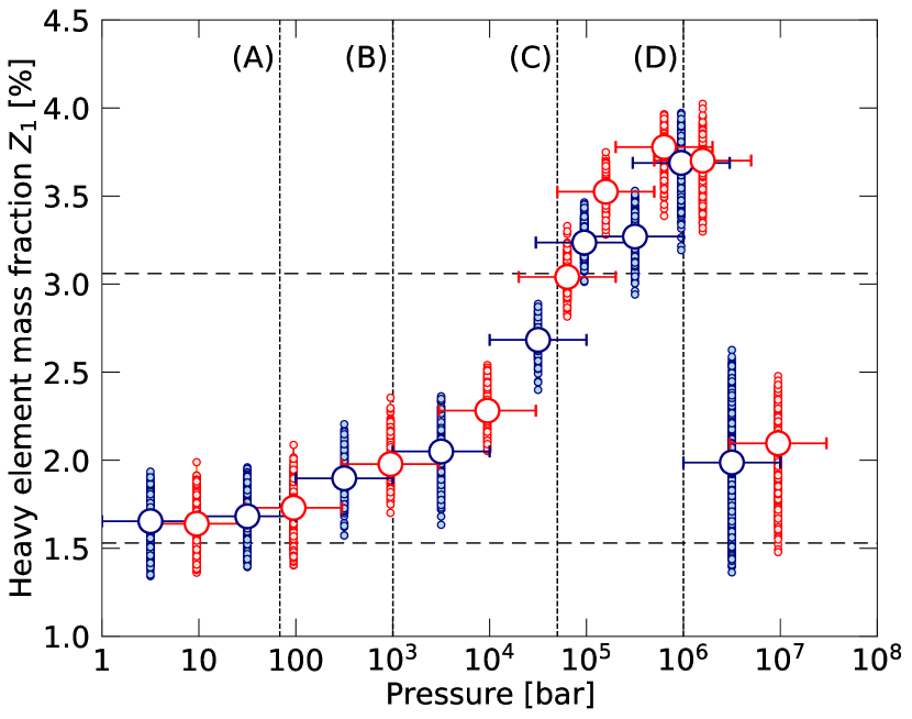
Figure 2: Upper panel: Five layer models of Jupiter’s interior. Lower panel: Effect of an EOS perturbation on heavy element abundance, $Z_{1}$. For 18 separate MC calculations, we lowered the density of our H-He EOS by 3% over a pressure interval from $P^{*}$ to $10\times P^{*}$ and studied how $Z_{1}$ increased. The small circles show individual $Z_{1}$ points while the large circle represent the ensemble average. The horizontal bar indicate the interval from $P^{*}$ to $10\times P^{*}$. The horizontal lines mark protosolar and twice protosolar abundances. The vertical lines A trough D are mark pressures of 68, 1005, $5\times 10^{4}$, and $10^{6}$ bar (1 Mbar = 100 GPa) that are also pointed out in the upper panel. (All points were calculate in the same way. Different colors were just introduced for clarity.)

We model Jupiter’s interior with five distinct layers that we illustrate in Fig. 2. The outer layer contains a mixture of molecular hydrogen, helium, and heavier elements. We derive its EOS by following Hubbard & Militzer (2016). We keep the entropy of this layer fixed by specifying the 1 bar temperature, 166.1 or 170 K. The helium mass fraction is held constant at the Galileo value of $\tilde{Y}_{1}=Y/(X+Y)=0.238$ (von Zahn et al., 1998). $Z_{1}$ represents the mass fraction of the heavy elements. The parameters $P_{\rm rain,1}$ and $P_{\rm rain,2}$ mark the beginning and ending pressures of the helium rain layer where the helium fraction, $Y/(X+Y)$, gradually rises from $\tilde{Y}_{1}$ to a higher value $\tilde{Y}_{2}$. Following Militzer et al. (2022), we adopt this functional form,

$$\tilde{Y}(P) = \tilde{Y}_{1}+x^{\alpha}\left[\tilde{Y}_{2}-\tilde{Y}_{1}\right]\;\;{\rm with}\;\;x=\frac{\log(P/P_{\rm rain,1})}{\log(P_{\rm rain,2}/P_{\rm rain,1})}$$ (16)

The $\tilde{Y}_{2}$ value is adjusted so that the planet overall (excluding heavy elements) has a helium fraction equal to the protosolar value of $Y_{0}/(X_{0}+Y_{0})=0.2777$ (Lodders, 2010). Inside of this layer is a thick, homogeneous, and convective layer of mostly metallic hydrogen that extends down to the core transition layer. The parameters $P_{\rm core,1}$ and $P_{\rm core,2}$ determine the beginning and ending pressures of this layer. We assume it to be stably stratified because the heavy element fraction increases gradually from $Z_{1}$ to $Z_{2}$. $Z_{2}$ is the heavy element abundance in the dilute core, which we assume to be homogeneous and convective. Together with the metallic hydrogen layer is contribution to generating Jupiter’s magnetic field (see analysis by Moore et al. (2022)).

To compare the different models, we define the core mass, $M_{\rm core}$, to be the mass inside of the pressure level, $P_{\rm core,2}$. The mass of the envelope, $M_{\rm env}$, is the mass outside the pressure level, $P_{\rm core,1}$. The remaining mass in between both pressures, is the mass of the core transition layer, $M_{\rm trans}$.

We employ the concentric Maclaurin spheroid (CMS) method (Hubbard, 2013) to construct a hydrostatic solution of a uniformly rotating oblate planet and then use the thermal wind equation to compute the contributions from the zonal winds. The CMS technique treats the effects of rotation nonperturbatively and is thus significantly more accurate than the traditional theory of figures (Zharkov & Trubitsyn, 1978) that starting from a nonrotating planets and then adds rotational effects using an expansion of different orders (Saumon & Guillot, 2004; Nettelmann et al., 2021).

We employ our quadratic Monte Carlo method to construct ensembles of Jupiter models by accepting and rejecting moves according to the $\exp(-\chi^{2}/2)$ function that includes four different terms, $\chi^{2}=\chi^{2}_{J}+\chi^{2}_{\rm H-He}+\chi^{2}_{\rm wind}+\chi^{2}_{\rm guide}$. The most important one measures the deviations of even and odd gravity harmonics between model predictions and the Juno measurements (Durante et al., 2020),

$$\chi^{2}_{J}=\sum\limits_{i=1}^{10}\left[\frac{J_{i}^{\rm model}-J_{i}^{\rm Juno}}{\delta J_{i}^{\rm Juno}}\right]^{2}\quad,$$ (17)

where $\delta J_{i}^{\rm Juno}$ are the 1-$\sigma$ uncertainties of the measurements.

While Eq. 17 is certainly the most important model generation criterion, there are a number of other well motivated constraints to consider (Militzer et al., 2019). For example, one would want to favor models with $P_{\rm rain,1}$ and $P_{\rm rain,2}$ value that are broadly compatible with phase diagram of H-He mixtures as derived by Morales et al. (2013). From the assumed molecular and metallic adiabats, we can infer the temperatures $T_{1}$ and $T_{2}$ that correspond to both pressures. For both pairs $P_{\rm rain,1}$-$T_{1}$ and $P_{\rm rain,2}$-$T_{2}$, we find the closest points on the immiscibility curve, $P^{*}_{1}$-$T^{*}_{1}$ and $P^{*}_{2}$-$T^{*}_{2}$, that minimize the following immiscibility penalty function,

$$\chi^{2}_{\rm H-He}=\sum\limits_{i=1}^{2}C_{P}\left|\frac{P^{*}_{i}-P_{i}}{P_{i}}\right|+C_{T}\left|\frac{T^{*}_{i}-T_{i}}{T_{i}}\right|\quad,$$ (18)

before we add the resulting minimum value to the total $\chi^{2}$. $C_{P}$ and $C_{T}$ are weights that must be balanced with those in other $\chi^{2}$ terms. We set $C_{T}/C_{P}=2$. Implicitly the $\chi^{2}_{\rm H-He}$ term also introduces a penalty for metallic adiabats that are too hot to be compatible with the assumed immiscibility curve. We chose not to square the individual terms in Eq. 18 because there is currently no agreement between theoretical and experimental results where in pressure-temperature space, hydrogen and helium become immiscible. Vorberger et al. (2007) had shown with ab initio simulation that hydrogen and helium are miscible at 8000 K. With more careful ab initio Gibbs free energy calculations, Morales et al. (2013) predicted hydrogen and helium to phase separate at approximately 6500 K for a pressure of 1.5 Mbar. Recent shock wave experiments by Brygoo et al. (2021) that combined Doppler interferometry and reflectivity measurements placed the onset of immiscibility at a much higher temperature of 10 200 K at 1.5 Mbar. Based on Militzer & Hubbard (2013), this corresponds to an entropy of 8.3 k_B/electron and imply that helium rain would set in as soon as a giant planet’s 1 bar temperature cools to 360 K. (Ab initio methods predict 180 K.) Helium rain would begin much earlier and cover a longer fraction of a giant planet’s lifetime. Fortney & Hubbard (2004) for example estimated that Jupiter’s 1 bar temperature only cooled by 10 K during the last 1.5 billion years. Also according to Wahl et al. (2021), helium rain would have already started on hot exoplanets in 9 day orbits like Kepler-85b but not on exoplanets in 1 and 3 days orbits such as WASP-12b and CoRoT-3b. Because the deviations of the ab initio predictions are unexpectedly large and these findings to not yet been reproduced with other laboratory measurements, we will employ the Morales et al. (2013) results when we evaluate the $\chi^{2}_{\rm H-He}$ term in Eq. 18 for this manuscript. Conversely, Miguel et al. (2022) does not invoke a term like Eq. 18 or a gradual change as in Eq. 16. Instead they employ a sharp transition from the molecular to the metallic hydrogen layer without incorporating predictions from ab initio simulations. This transition occur between 2 and 5 Mbar in most models.

Third we add a penalty term (Militzer et al., 2022),

$$\chi^{2}_{\rm wind}=\frac{1}{m}\sum\limits_{i=1}^{m}\left\{\begin{matrix}\left[H(\mu_{i})-H_{\rm max}\right]^{2}&{\rm if\,\,}H(\mu_{i})>H_{\rm max}\\ 0&\;\;\;\;\;\;\;\;\;\;\;\;\;{\rm if\,\,}H_{\rm min}\leq H(\mu_{i})\leq H_{\rm max}\\ \left[H_{\rm min}-H(\mu_{i})\right]^{2}&{\rm if\,\,}H(\mu_{i})<H_{\rm min}\\ \end{matrix}\right.\quad,$$ (19)

that keeps the depth of our winds, $H$, within perscribed limits of $H_{\rm min}=1500\,$km and $H_{\rm max}=4500\,$km to keep them broadly compatible with earlier predictions (Guillot et al., 2018). We evaluate them at $m=61$ equally spaced $\mu$ points between –1 and +1 with $\mu=\cos(\theta)$ and $\theta$ being the colatitude. We directly use the observed cloud-level winds from Tollefson et al. (2017) but then assume the wind depth to be latitude dependent. Alternatively one can allow the winds on the visible surface to deviate from the observations and keep the wind depth the same for all latitudes. Both types of wind solutions are compared in Militzer et al. (2022).

We solve the thermal wind equation (Kaspi et al., 2016) to derive the density perturbation, $\rho^{\prime}$,

$$\frac{\partial\rho^{\prime}}{\partial s}=\frac{2\omega}{g}\frac{\partial}{\partial z}\left[\rho u\right]\quad,$$ (20)

for a rotating, oblate planet (Cao & Stevenson, 2017) in geostrophic balance. $z$ is the vertical coordinate that is parallel to the axis of rotation. $s$ is the distance from the equatorial plane along a path on an equipotential. $\rho$ is static background density and $g$ is the local acceleration. We obtain both from our CMS calculations of a particular model, which means our wind model and the interior structure are selfconsistent. $u$ is the differential flow velocity with respect to the uniform rotation rate, $\omega$. We represent $u$ as a product of the surface winds, $u_{s}$, from Tollefson et al. (2017) and a decay function of $\sin^{2}(x)$ form from Militzer et al. (2019) that keeps the wind speeds initially constant before they decay over a small depth interval. This is consistent with assumptions made by Dietrich et al. (2021) and Galanti & Kaspi (2021) while in Kaspi et al. (2018) and Miguel et al. (2022) a gradual decay of the wind speed with depth is assumed.

We integrate the density perturbation, $\rho^{\prime}$, to determine the dynamic contributions to the gravity harmonics before combining them with the static gravity harmonics that we have obtained from the CMS calculation, $J_{n}^{\rm model}=J_{n}^{\rm static}+J_{n}^{\rm dynamic}$. The resulting harmonics are then compared with the Juno measurements in Eq. 17. We work with the error bars of the Juno measurements, $\delta J_{i}^{\rm Juno}$ directly since we construct selfconsistent models in which wind terms can compensate for variations in the interior structure. This is one of the main differences to the recent work by Miguel et al. (2022) who performed interior and wind calculations separately and increased the Juno error bars by a factor of 30 to represent an unknown contribution to even harmonics that comes from the winds. The other main difference is that we used the nonperturbative CMS approach while Miguel et al. (2022) relied on the 4th order theory of figures method but then compute a correction for a subset of models.

Finally we add the penalty term,

$$\chi^{2}_{\rm guide}=C\left\{\begin{matrix}\left[p_{\rm min}-p\right]^{2}&{\rm if\,\,}p<p_{\rm min}\\ 0&{\rm otherwise}\\ \end{matrix}\right.\quad,$$ (21)

that help us guide the Monte Carlo ensemble to reach and remain in parameter region with $p\geq p_{\rm min}$ that we consider physical. (Similar terms can assure $p\leq p_{\rm max}$.) We find such a soft approach to work better then a hard constraint that would reject any model that violates the condition, $p\geq p_{\rm min}$. Still we set $C$ to a high value like 1000 to assure compliance. We verify that $\chi^{2}_{\rm guide}=0$ for models that we publish. $Z_{1}\geq Z_{\rm protosolar}$ is an obvious condition to satisfy but we also require $Z_{2}\geq Z_{1}$ and $S_{2}\geq S_{1}$.

The Juno gravity measurements (Folkner et al., 2017; Iess et al., 2018; Durante et al., 2020) have reached a very high degree of accuracy and the fact that we employed the error bars directly, rather than inflating them, underlines the need to an efficient sampling method that we provide with our quadratic Monte Carlo approach.

Some interior parameters are allowed to vary freely during the Monte Carlo calculations while others are others constrained by observations. For example, we do not vary the helium fractions, $Y_{1}$ and $Y_{2}$ because $Y_{1}$ is constrained by measurements of the Galileo entropy probe and $Y_{2}$ is derive so that the planet overall has a protosolar $\tilde{Y}$. The heavy elements fractions, $Z_{1}$ and $Z_{2}$ are employed so that the model matches the planet’s mass and $J_{2}$. During the Monte Carlo procedure, we only vary the four pressures, $P_{\rm rain,1}$, $P_{\rm rain,2}$, $P_{\rm core,1}$, $P_{\rm core,2}$, the helium rain exponent $\alpha$, the entropy of the deep interior, $S_{2}$, and the depth of the winds, $H(\mu_{i})$. We do not introduce a prior distribution or apply any hard constraints to these four pressure values. Their posterior distribution is just a result of the different $\chi^{2}$ terms that we have described in this section.

3 Results

3.1 Application to Ring Potential

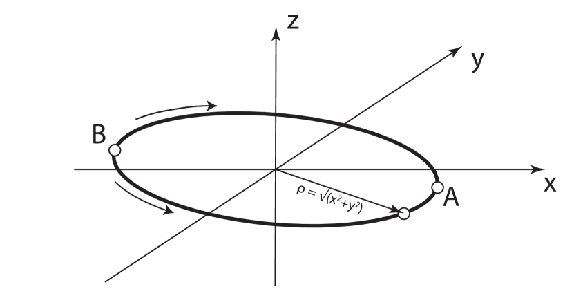
Figure 3: Illustration of the ring potential, $V(\vec{r}=(x,y,z))$, that we constructed to study how well different MC algorithms work in confined geometries. By construction, the potential becomes small if the distance $\rho$ equals a given radius, $R$. We slightly tilted the ring to illustrate the effect of the last term in Eq. 22 that breaks the axial symmetry by lowering the potential for positive $x$ values.

In order to study how our QMC method performs in confined geometries, we constructed the following ring potential,

$$V(\vec{r})=(2m)^{2m}\left[(\rho-R)^{2m}+\sum_{i=3}^{N}r_{i}^{2m}\right]-Cr_{1}\;\;,$$ (22)

where $\vec{r}=\{r_{1},\ldots,r_{N}\}$ is a vector in the $N\geq 2$ dimensional parameter space. $\rho=\sqrt{r_{1}^{2}+r_{2}^{2}}$ is the distance from the origin in the $r_{1}$-$r_{2}$ plane. The first term ensures that the potential is only small along a ring of radius, $R$, in $r_{1}$-$r_{2}$ space as we illustrate in Fig. 3. The second term keeps the magnitude of all remaining parameters, $r_{3\ldots N}$ small. Increasing the positive integer, $m$, allows us to make the potential more confining by making the potential walls around the ring steeper. Finally we introduce the last term to break axial symmetry. Typically we set C to small value like 0.01 so that the potential minimum is approximately located at point $\vec{A}=(+R,0,\ldots)$ while the potential is raised at opposing point $\vec{B}=(-R,0,\ldots)$. The prefactor of the first term in Eq. 22 is introduced so that the location of potential minimum does not shift much with increasing $m$.

For this test case, we insert the ring potential into the Boltzmann distribution in Eq. 13. If we initialize an ensemble of walkers in the vicinity of point $\vec{B}$, the algorithm has no choice but to travel along the ring until it reaches the area of point $\vec{A}$ where the sampling probability is highest, the most relevant states will be sampled, and only then the block averages will start to stabilize.

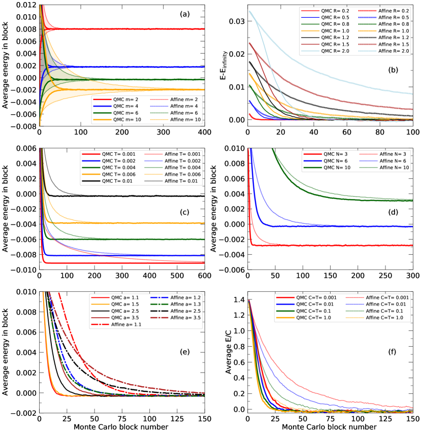
Figure 4: Performance comparison between affine MC and our quadratic MC methods. The average potential energy in a MC block is plotted as function of block number in order to illustrate how long it takes for either method to converge. For all parameters considered here, the QMC method does so more efficiently. In panel (a), two curves are plotting for every method. Tose that converge from above represent MC ensembles that were initialized from the high-energy point $\vec{B}$ (see Fig. 3) while those converge from below where started from the low-energy point $\vec{A}$. In all following panels, we only show ensembles that were initialized near $\vec{A}$. In panel (b), the final, converged energy has been subtracted for clarity. In panel (f), the energy has been divided by constant $C$. (To reduce the noise, 1000 independent MC simulations have been averaged to generate each curve.)

In Figs. 4 and 5, we compare the performance the affine MC and our quadratic MC methods under different conditions. As our baseline case, we set $N=6,m=6,R=1,C=0.01,T=0.01,$ and $a=2.5$. In every block, we attempt to make $10^{3}$ individual moves. In most cases, we initialize the ensemble of MC walkers near point $\vec{B}$, which means average block energy will decrease as the ensemble travels towards the potential minium near point $\vec{A}$ (see Fig. 3). In Fig. 4a, we compare how long that takes for different values $m$. Increasing $m$ makes the potential walls steeper, which causes both methods to converge more slowly. However, in comparison, the QMC method perform significantly better. For $m=10$, it only takes 54 blocks for it converge within 2$\times$10^-4 of the final energy while it takes 308 blocks for the affine MC method to do so. In Fig. 4a, we also show results from simulations that initialized the ensemble of walker at the low-energy point $\vec{A}$. The convergence rates are similar to those before but block averages now converge to the final block energy from below.

In Fig. 4b, we compare the performance of both method for different ring radii, $R$. For a very small value of 0.2, both methods converge equally fast. With increasing radius, it takes the affine MC method much longer than our QMC method to do so. When we lower the temperature from 0.01 to 0.001, we find a similar behavior in Fig. 4c. A lower temperature makes the potential appear more confining, which delays the convergence of the affine MC method dramatically.

In Fig. 4d, we compare the convergence for different spatial dimensions $N$. For $N=3$ and 6, the QMC method converges faster but for $N=10$, the behavior is fairly similar to that of the affine MC method, and it takes both methods longer to converge than for smaller $N$.

In Fig. 4e, we test the dependence on the scaling parameters $a$. For the QMC method, values between $a=1.1$ and 1.5 yield optimal results. For the affine methods, $a\approx 1.3$ is optimal but even then it converges only half as fast approximately as our quadratic method.

Finally in Fig. 4f, we vary the temperature that enters the MC calculation via the Boltzmann factor. Since we are interested in the effects of ring term in Eq. 22 , we set the constant $C$ equal temperature $T$ for this particular analysis. A change in $C=T$ recalibrates the strength of the ring term in Eq. 22 in relation to the linear term. For small $C=T$ values, the confining effect of the potential increases, which foremost delays the convergence of the affine method.

Summarizing one found that for our ring potential, our QMC method performed significantly better than the affine MC method for most conditions. In a few cases like large spatial dimension $N$, the performance was found to be similar.

Figure 5: Autocorrelation function (panel a) and error bar from blocking analysis (panel b) of affine and quadratic MC calculations. In panel (c), we compare the Monte Carlo error bar from the block analysis and the time it take the ensemble to travel around the ring. The number of attempted MC moves was the same in all cases. The symbols correspond to different stretch factors, $a$, given in the legend. Results for various numbers of walkers are shown, $N_{W}$=7, 9, 11, 15, 19, 31, 51, and 200. The blue symbols show results derive with the affine method for $a$=1.2, 1.5, 2.0, and 2.5. The thin, medium thick, and thick blue lines represent results with $N_{W}$=7, 19, and 200 walkers, respectively. The remaining symbols show results from our quadratic MC method with uniform (red) and Gaussian (green) sampling of the $t$ space. The medium thick and thick red lines show the best QMC results for $N_{W}$=11 and 15, respectively. Compared the affine method, our QMC method requires a approximately travel time half as long and leads to error bars half as large if $N_{W}=7\ldots 19$ and $a=0.3\ldots 1.5$ are used.

In Fig. 5, we study autocorrelations of the block energy for our base case parameters, $N_{W}$=7 walkers, and the two stretch parameter $a=1.5$ and 2.5. For this analysis, we removed the transient part of the calculation (see Fig. 4) where the block energies have not yet converged. Fig. 5a shows that the autocorrelation functions of affine MC energies decay much more slowly than that of the QMC energies. Based on the integrals under the plotted curves, we estimate the autocorrelation time to be 79000 and 123000 MC moves for the affine method with a=1.5 and 2.5 respectively but only 12000 and 19000 MC moves for the QMC method (with linear sampling of $P(t)$).

We also performed a block analysis for these four calculations (Allen & Tildesley, 1987; Martin et al., 2016). In Fig. 5b, we plot the error bars that emerged from the blocking analysis when individual block energies are combined into longer and longer blocks. All curves show a plateau that indicates that the blocks were chosen to be sufficiently long for the block averages to be uncorrelated. The affine MC method yielded an energy of $(-3.02\pm 0.12)\times 10^{-4}$ and $(-3.11\pm 0.17)\times 10^{-4}$ for $a=1.5$ nd 2.5 respectively. With the QMC method, we obtained $(-3.007\pm 0.051)\times 10^{-4}$ and $(-3.013\pm 0.063)\times 10^{-4}$ for the two $a$ values respectively. All averages are compatible with one another. For the same calculation duration, the QMC method yielded an error bar that is 2.5 smaller. This is in agreement with observation that its autocorrelation time is approximately six times shorter.

In Fig. 5c, we compare the performance of the affine method with that of our QMC method using linear and Gaussian $t$ sampling. It is our goal of this quantitative analysis is give some guidelines how the stretch factor, $a$, and the numbers of walkers, $N_{W}$, should be chosen. Goodman and Weare recommended setting $a=1.5$ and did not make a recommendation for $N_{W}$ besides choosing it to be large. (E.g. Miguel et al. (2022) employed 512 walkers to sample a 7 dimensional parameter space.) For the ring potential with $T=0.01$, $N=6$, $m=6$, $R=1$, we consider value of the stretch factor $a$ from 0.3 to 2.5 to explore the perform of all three methods even though we consider value $a<0.5$ and $a>1.5$ poor choices. (The affine method requires $a>1$ while the others do not.)

A large number of walkers introduces diversity, which helps to explore the parameter space. On the other hand, if the number of walkers is chose to be too be large, one would expect to algorithm to have difficulties to explore all relevant areas of the parameter space efficiently. In principle one would expect the number of walkers scale with the dimensionality of the space.

In our view, an efficient MC method should have two properties. It should travel effectively from improbable parameter regions to the relevant ones. Once there, it should yield to small error bars for the estimated averages. The two axes of Fig. 5c measure both properties. On the Y axis, we plot the error bar that we obtained with the blocking analysis for long MC calculations (one per pair of $a$ and $N_{W}$ parameters) with 10¹⁰ moves. We initialized the ensemble near low-energy point $\vec{A}$ because, for the error bar calculations, we are are not interest in the time it take the ensemble around the ring. To determine the travel time, we performed 10³ separate but shorter calculations with 10⁷ moves starting from point $\vec{B}$. Every time, we recorded the ring travel time that we define to be average number of MC moves that are required for the energy in the ensemble to reach the mid value between the initial potential energy and final converged value that we quoted above. The ring travel time and the MC error bar both have statistical uncertainties, which introduces noise into Fig. 5c. Still a number of trends emerge clearly.

If a unreasonably number of walkers like $N_{W}=200$ is chosen for the affine method, the ring travel time becomes very large and approaches 10⁶ MC moves. To a lesser degree, this trend is also seen for the QMC method. On the other hand, the computed error bars do not suffer from choosing $N_{W}$ very large. So employing a very large ensemble of walkers yields comparable but not smaller error bars than employing more modest numbers of walkers.

If only 7 walkers are used for the affine method, the ring travel times become very reasonable but resulting MC error bar becomes very large. The best performance is seen for $N_{W}=9\ldots 19$ and $a$=1.5, which yields an average ring travel time of $8\times 10^{4}$ moves and an error bar of $2.5\times 10^{-6}$.

For the same number of MC moves, our QMC method yields error bars half the size of the affine method and ring travel times that are approximately half as long. We see no particular advantage of using the Gaussian $t$ sampling method. The linear $t$ sampling method yields the very good results over a wide range $a$ values from $a=0.3\ldots 1.5$ and $N_{W}$=7 $\ldots$ 19. The average travel time is only $4\times 10^{4}$ moves and the error bar is $1.1\times 10^{-6}$. Based on this analysis, we recommend setting $N_{W}=2N+1\ldots 3N+1$ in general.

3.2 Comparison between Quadratic Sampling and Walk Moves

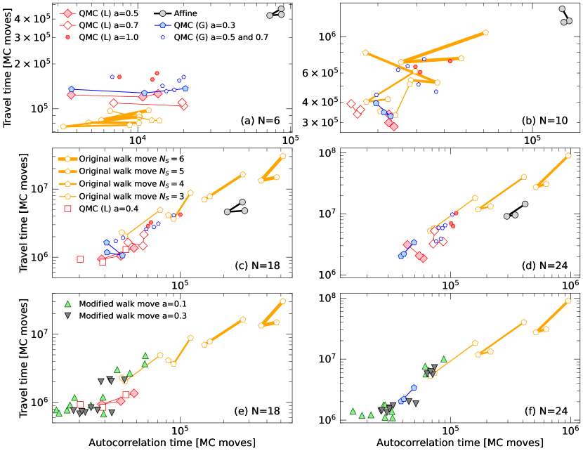
Figure 6: Travel and autocorrelation times computed for the ring potential in dimensions $N=6$, 10, 18 and 24. An efficient algorithm makes both as short as possible. Panels (a)-(d) compare results from the affine, quadratic and the original walk method ($a=1$). For a low dimension of $N=6$, the walk moves perform best regardles whether subset size, $N_{S}=3\ldots 6$, is chosen but the original walk moves are not competitive for $N>10$. Panels (e) and (f) include results from the modified walk method for $N=18$ and 24 because we found that choosing a scale factor $a\ll 1$ increases the sampling efficiency. Symbols were chosen consistently across all panels. So QMC (L) and (G) label results from the quadratic MC method with linear and Gaussian $t$ sampling respectively. The symbols distinguish results that were obtained with different $a$ parameters.

In Fig. 6, we compare the travel and autocorrelation times from the walk method for the ring potential in $N=6$, 10, 18 and 24 dimensions with results obtained affine and quadratic methods using linear and Gaussian $t$ sampling. For every dimension $N$, we performed independent calculations for $N_{W}=N+2,3N/2,$ and $2N$. For the affine method, we fix $a=1.5$ but for the quadratic MC method, we considered $a=\{0.1,0.2,0.3,0.4,0.5,0.7,1.0\}$ for the linear $t$ sampling and $a=\{0.3,0.5,0.7\}$ for the Gaussian $t$ sampling. For original walk method, we chose $N_{S}=3,4,5,$ and 6 for the size of the subset of guiding walkers. We noticed that choosing $N_{S}$ larger made such calculations very inefficient since it led to drastic increases in the travel and autocorrelation times for $N\geq 10$ as panels (b)-(d) of Fig. 6 illustrate. For lower dimension of $N=6$, however, the results of the original walk methods are very good. Panel (a) shows that the travel time can be up to 25% shorter than that of the quadratic sampling method.

Already for $N=10$ dimensions results from the original walk method fall behind those of the quadratic sampling method. For $N=18$ and 24, this trend continues and for a subset size of $N_{S}=6$, the original walk method yields longer travel and autocorrelation times than even the affine method, regardless what ensemble size, $N_{W}$, is employed. This increase in travel and autocorrelation times led us to introduce the scaling factor $a$ into Eq. 15. Choosing small values of $a=0.1$ or 0.3 enabled us to obtained travel and autocorrelation times with the walk method that are at par or shorter than those of the quadratic sampling method as panels (e) and (f) of Fig. 6 illustrate. In the next section, we will analyze how valuable our scaling factor $a$ can be for the sampling of the Rosenbrock density.

3.3 Sampling the Rosenbrock Density

Figure 7: Energy autocorrelation time, energy error bar and acceptance ratios derived for the Rosenbrock density being sampled for $A=100$ and 10000 with the affine method, the quadratic MC method with linear (QMC L) and Gaussian (QMC G) $t$ sampling as well as with the modified walk method. The symbols distinguish results that were obtained with different $a$ parameters.

Following Goodman & Weare (2010), we also applied our methods to sampling the 2d Rosenbrock density,

$$\pi(x_{1},x_{2})\propto\exp\left\{-\frac{A\left(x_{2}-x_{1}^{2}\right)+(1-x_{1})^{2}}{B}\right\}\quad,$$ (23)

which carves a narrow curved channel into the $(x_{1},x_{2})$ landscape. $B$ effectively plays the role of temperature. First we set $A=100$ and $B=5$ to be consistent with Goodman & Weare (2010) but then we also increase $A$ to 10000, while leaving $B$ unchanged, which makes the channel even narrower and makes sampling it yet more challenging.

For both $A$ values, we performed a series of independent MC calculations with 10⁷ blocks, each consisting of 10³ individual moves. We compared the performance of ensembles with $N_{W}=\{3,4,5,6,8,10,20\}$ walkers for the following four methods: For the affine method, we compared the $a$ values $\{1.2,1.5,2.0,2.5\}$, for the quadratic MC with linear and Gaussian $t$ sampling we considered $a=\{0.3,0.5,0.7,1.0,1.2,1.5,2.0\}$ respectively. For the modified walk moves, we studied the combined ranges of $a=\{0.1,0.3,0.5,1.0,1.2,1.5,2.0,3.0\}$ and $N_{S}=\{4,5,6,10\}$ under the condition $N_{S}<N_{W}$.

The results are summarized in Fig. 7 where we plot the autocorrelation time, $\tau$, and the error bar, $\sigma$, that we computed with the blocking method. Both were derived from average energy that we computed for everyone of the last 80% of the 10⁷ blocks. We define an energy for the Rosenbrock density, $E(x_{1},x_{2})=-\ln\pi(x_{1},x_{2})$, using the analogy between Eq. 23 and the Boltzmann factor with $k_{b}T=1$.

Despite conserable noise in Fig. 7, one can identify the expected scaling of $\tau\sim\sigma^{2}$ between the auto correlation time, $\tau$, and the computed error bar, $\sigma$. An optimal algorithm would make both as small as possible. As expected, both values increase considerably for all algorithms if one raises $A$ from 100 to 10000 because it narrows the channel of the Rosenbrock density, which makes sampling it yet more difficult.

We find the affine method yields the largest energy error bars among all methods regardless of which $a$ value is employed. The performance of the modified walk method strongly depends on the choice of $a$, which renders the our modification in Eq. 15 important. For the sampling of the Rosenbrock density, we find that $a$ values larger than 1 perform the best, even though they yield an rather low acceptance ratio of only 2$\times$10^-3 as the lowest panel of Fig. 7 illustrates. However, if $a$ is choosen too large, the acceptance ratio decreases below 10^-3 and the autocorrelation time increases because too few of the large steps get accepted.

We found that the quadratic MC method samples the Rosenbrock density most efficiently. For $A=10000$, the shortest autocorrelation time were approximately four times short than the best results that we obtained with the modified walk method. In Fig.  7, we highlighted some of the most favorable results that were obtained with Gaussian $t$ sampling for $a=1.5$ and linear $t$ sampling for $a=2.0$. The acceptance ratio were again rather low and ranged from 0.01 to 0.03 only. This means for challenging sampling problems like the Rosenbrock density, one may want invest in determining an optimal or at least a reasonable choice for the scaling parameter $a$.

3.4 Predictions for Jupiter’s Interior

We applied our QMC algorithm to generate three different ensembles of interior models under the assuptions in Sec. 2.4. The resulting posterior distributions are shown in Figs. 8 and 9 while averages and standard deviations of different parameters are given in Tab. 1. The three ensembles are:

1. This is our reference ensemble of the five-layer models from Militzer et al. (2022).

2. We increased the interior entropy by increasing the temperature at 1 bar from the Galileo measurements of 166.1 K to 170 K, which reduces the density of H-He mixtures in the molecular layer. At the lowest pressures, where H-He mixture behaves like an ideal gas, this translates into a density reduction of 2.3%. At higher pressure, the reduction is smaller because the systems is more electronically degenerate.

3. Finally we made a change in our equation of state of H-He mixture and reduce the density by 3% in the region from $P^{*}=10$ to 100 GPa but employ a 1 bar temperature of 166.1 K.

Table 1: Ensemble averages and standard deviations of different interior model parameters. Machine-readable data files for a representative model of each ensemble are included in the supplemental material.

Parameter	Reference	$T_{\rm 1bar}=170\,$K	3% density
	ensemble	ensemble	reduction
$Z_{1}$ [%]	1.56 $\pm$ 0.05	2.03 $\pm$ 0.06	3.27 $\pm$ 0.04
$P_{\rm rain,1}$ [GPa]	98 $\pm$ 16	107 $\pm$ 15	95 $\pm$ 11
$P_{\rm rain,2}$ [GPa]	445 $\pm$ 19	314 $\pm$ 19	315 $\pm$ 13
$Z_{2}$ [%]	18.3 $\pm$ 0.3	19.5 $\pm$ 0.3	20.6 $\pm$ 0.3
$P_{\rm core,1}$ [GPa]	786 $\pm$ 38	979 $\pm$ 44	1389 $\pm$ 48
$P_{\rm core,2}$ [GPa]	2054 $\pm$ 106	1946 $\pm$ 96	1811 $\pm$ 63
$M_{\rm Z,total}\,[M_{E}]$	25.08 $\pm$ 0.06	25.92 $\pm$ 0.06	26.90 $\pm$ 0.05
$M_{\rm core}\,[M_{J}]$	0.20 $\pm$ 0.02	0.22 $\pm$ 0.02	0.25 $\pm$ 0.01
$M_{\rm trans}\,[M_{J}]$	0.34 $\pm$ 0.03	0.25 $\pm$ 0.03	0.10 $\pm$ 0.02
$M_{\rm env}\,[M_{J}]$	0.49 $\pm$ 0.02	0.53 $\pm$ 0.02	0.65 $\pm$ 0.01

Most notably these two density changes increase the mount of heavy elements, $Z_{1}$, but they also introduce additional flexibility into our models and thereby widen the allowed region of other model parameters, as the larger standard deviations in Tab. 1 confirm.

One finds that an increase of the 1 bar temperature from 166.1 to 170 K leads to an modest increase in $Z_{1}$ from $\sim$1.6% to $\sim$2.0% while the 3% density reduction leads to a much larger increases $Z_{1}$ to $\sim$3.3%, effectively doubling the amount. We find increases of similar magnitude for the heavy elements abundance of the dilute core region, $Z_{2}$, from 18.3% to 19.5% to 20.6% when the three ensembles are compared. Conversely, the ending pressure for the helium rain layer, $P_{\rm rain,2}$, decreases from $\sim$445 in our reference ensemble to $\sim$315 GPa in other two ensembles.

Fig. 8 shows that $Z_{1}$ is positively correlated with $P_{\rm rain,2}$ because an increase in $P_{\rm rain,2}$ means helium is sequestered to deeper layers and the resulting density reduction over 100–300 GPa pressure interval is compensated by a modest increase in $Z_{1}$. In comparison, the correlation between $Z_{1}$ and the starting pressure of helium rain layer, $P_{\rm rain,1}$, is rather weak because typical values for helium rain exponent are $\alpha\gtrsim 3$ so that the helium concentration does not vary much near $P_{\rm rain,1}$. This is also the reason why $P_{\rm rain,1}$ does not strongly correlate with other model parameter.

Fig. 8 further shows that, within a given ensemble, $Z_{1}$ does not correlate strongly with $Z_{2}$ nor with core pressures, $P_{\rm core,1}$ and $P_{\rm core,2}$. Still, $Z_{1}$ is positively correlated with the magnitudes of $\left|J_{4}\right|$, and $\left|J_{6}\right|$ while there is no apparent correlation with $\left|J_{8}\right|$. $Z_{2}$ and $P_{\rm core,1}$ correlate in the same way with these three gravity coefficients but strengths of their correlation are much higher. The extended dilute core is the main feature of our feature of our five layer models that enables us to fit $J_{4}$ and $J_{6}$ by distributing heavy elements over a wider range of radii than was possible with compact core assumption. So one expects strong correlations of $J_{4}$ and $J_{6}$ with $Z_{2}$ and $P_{\rm core,1}$ that control the heavy element distribution in the core region.

$Z_{2}$ positively correlates with $P_{\rm core,2}$ because an increase of $P_{\rm core,2}$ effectively shrinks the size of the dilute core which is then compensated by an increase in $Z_{2}$. As expected, one finds that $P_{\rm core,1}$ and $P_{\rm core,2}$ are negatively correlated so the combined mass of heavy elements in the core and core transition layer is kept approximately constant.

In the bottom row of Fig. 8 we compare the Juno measurements of gravity harmonics $J_{4}$–$J_{8}$ with the histogram of the computed ensembles. $J_{4}$ is well matched by all three ensembles, which is a consequence of adopting a dilute core. Matching $J_{6}$ is still not straightforward. Models that reduce the density by 3% are symmetrically distributed around the measured $J_{6}$ value. There is also good overlap with models that adopted a 1 bar temperature of 170 K. Most models with a 1 bar temperature of 166.1 K exhibit a larger $J_{6}$ value than was measured. Still as we have shown in Militzer et al. (2022), there are models in the 166.1 K ensemble that match $J_{6}$ exactly but there are also many others that yield higher values. In comparison, matching $J_{8}$ poses no challenge.

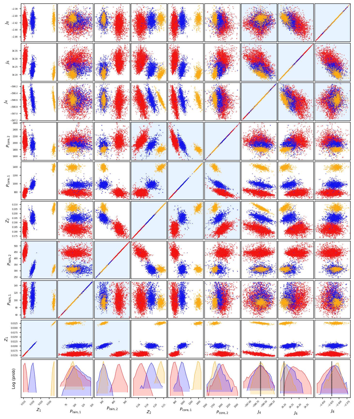
Figure 8: Posterior distribution of the three different QMC ensembles: 1) The red circles represent our reference ensemble of five layer models with a dilute core. 2) We made Jupiter’s interior slightly hotter by increasing temperature at 1 bar from Galileo measurement of 166.1 to 170 K (blue symbols). 3) We reduced the density of the H-He mixture by 3% over the pressure interval from 10 to 100 GPa (orange circles). $Z_{1}$ and $Z_{2}$ are mass fractions of heavy element. The four pressure values are given in units of GPa. The values of the gravity harmonics, $J_{4}\ldots J_{8}$, have all been multiplied by 10⁶. The vertical dashed lines indicate the Juno gravity measurements.

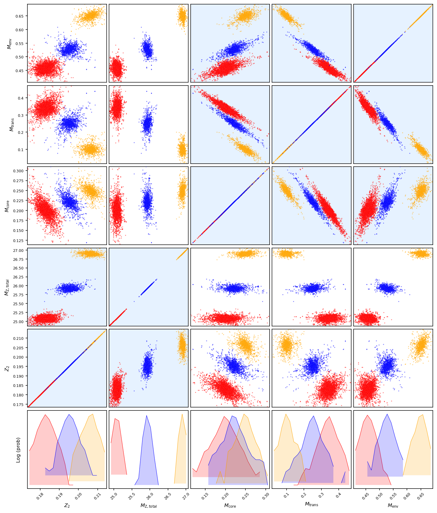
Figure 9: Posterior distribution for the three different QMC ensembles that we show in Fig. 8. Here we plot correlations between heavy elements fraction in the core, $Z_{2}$, the total amount of heavy elements in the planet, $M_{\rm Z,total}$, and the masses of the core, the core transition layer and the envelope. (The values of three masses were divided by the planet’s total mass so that they add up to 1.) The probability distributions of all variables are shown in the bottom panels on a logarithmic scale.

In Fig. 9, we investigate correlations between the core mass fraction, $Z_{2}$, the planet’s total budget of heavy elements, and the masses of the three layers. (Combined they match the planet’s total mass, $M_{J}$.) When we increase the 1 bar temperature (or lower the density by 3% in the 10–100 GPa region), the total amount of heavy elements increase modestly from 25 to 26 (or 27) Earth masses. This is a modest increase compared to 8–39 Earth mass range that Saumon & Guillot (2004) had obtained by considering a plethora of tabulated EOS models for hydrogen. Our heavy element abundances are a bit lower than the 28–32 Earth mass range that Nettelmann et al. (2012) because a compact core and a higher interior temperature profile were assumed.

When we switch between our three ensembles from 1 to 2 (or to 3), the mass of the dilute core increases from 0.20 to 0.22 (or to 0.25) $M_{J}$. The mass of the core transition layer shrinks drastically from 0.34 to 0.25 (or to 0.10) $M_{J}$ as $P_{\rm core,1}$ increases and $P_{\rm core,2}$ decreases. By definition, a rise in $P_{\rm core,1}$ also increases the mass envelope (that include molecular, helium rain, and metallic hydrogen layers) from 0.49 to 0.53 (or to 0.65) $M_{J}$. Switching from ensemble 1 to 2 or 3 leads to a reduction in the size of the dilute core because one lowers the density in the outer region of the planet. This is consistent with earlier modeling work that predicted small or negative heavy elements abundances (Hubbard & Militzer, 2016) because no dilute core was considered.

Fig. 9 illustartes that, within each ensemble, the mass of the transition layer negatively correlates with the masses of the core and that of the envelope. It provides a way to match the total mass of the planet. More surprising is, however, the masses of the core and the envelope are positively correlated. This is consistent with the trend one sees in the first column in Fig. 9. When $Z_{2}$ increases within a particular ensemble, the core mass drops, and the envelope mass increases slightly while the mass of the transition layer remains approximately unchanged.

3.5 Equation of state perturbations

Equations of state of materials at high pressure have been studied with laboratory measurements (Brygoo et al., 2015) and ab initio computer simulations (Militzer, 2009; Hu et al., 2011; McMahon et al., 2012; Militzer et al., 2021). At the same time, it has been a major challenge to the match Jupiter’s $J_{4}$ and $J_{6}$ with interior models that an rely on a physical equation of state for H-He mixtures and, for the molecular envelope, yield at least a protosolar abundance of heavy elements of $Z_{\rm protosolar}=1.53$% according to Lodders (2010) who derived the present-day solar abundances in Tab. 2 by combining spectroscopic measurements of the solar photosphere with laboratry measurements of CI chondrite meteorites. Over time, heavy elements diffuse slowly towards a stars interior because of gravitational forces. Lodders (2010) represent this process by applying a uniform factor of $10^{0.053}$ to obtain the protosolar from the solar abundances. Most of the heavy elements mass comes from just 7 elements that are listed in Tab. 2.

Table 2: Mass fractions in % of different heavy elements according to measurements and various models. The second and third column lists the solar and protosolar abundances from Lodders (2010). The columns four and five show two compositional models for Jupiter. The last column lists one possible interpretation (Hubbard & Militzer, 2016) of measurement of the Galileo entry probe (Wong et al., 2004).

	Present-day	Inferred	3-fold proto-	4-fold CO	Galileo
Element	solar	protosolar	solar model	model for	entry
	abundances	abundances	for Jupiter	Jupiter	probe
O	0.63	0.71	2.13	1.50	0.29
C	0.22	0.25	0.75	1.00	1.06
Ne	0.17	0.19	0.02	0.02	0
Fe	0.12	0.14	0.41	0.14	0
N	0.07	0.08	0.24	0.08	0.35
Si	0.07	0.08	0.24	0.08	0
Mg	0.06	0.07	0.20	0.07	0
Others	0.07	0.08	0.24	0.08	0
Total	1.41	1.53	4.2	2.9	1.7

Note. — Some rounding errors are to be expected.

In Jupiter’s atmosphere, the noble gas neon has been measured to be nine-fold depleted (Mahaffy et al., 2000) compared to the protosolar abundance. It is assumed that neon partitions strongly into the helium droplets when hydrogen and helium phase separate at megabar pressures (Roulston & Stevenson, 1995; Wilson & Militzer, 2010). While the helium depletion is important for interior models, neon only contribute 11% to the solar heavy element budget.

While there is significant uncertainty in the data that have been obtained for heavy element abundances in Jupiter’s atmosphere, one can make a number of plausible assumptions and then compare them with the predictions from interior models (Nettelmann et al., 2012). Here we compare the predictions from our interior models with three abundance models in Tab. 2:

(1) First one can assume all heavy elements are uniformly enriched to their 3-fold protosolar abundance (Owen et al., 1999) while neon has been 9-fold depleted. This yields $Z^{\rm(3fold)}\approx 4.2\%$. This assumes the measured enrichment of carbon, nitrogen, and sulfur applied to all heavy elements even though their respective condensation temperatures are very different, which may pose a challenging if one assumes they were delivered along with solid planetesimals. On the other hand, the near uniform enrichment of the noble gases suggests that direct capture of nebula gas may have played a role (Lodders, 2004). Laboratory condensation experiments (Notesco et al., 2003) showed the preferred way to condense noble gases is to trap them in amorphous ice (Bar-Nun et al., 2007) but these measurements also demonstrated the corresponding trapping rates are nonuniform.

(2) It has also been proposed that oxygen and carbon atoms were delivered in equal numbers in form of carbon monoxide (Helled & Lunine, 2014). If one assumes the measured 4 times protosolar abundance of carbon of reflects this delivery processes, we obtain $Z^{\rm(CO)}\approx 2.9$% while we have included all other elements, except neon, in protosolar proportions.

(3) Finally we can take the measurements of the Galileo entry probe with its subsolar water abundance at face value, $Z^{\rm(Gal)}\approx 1.7$%. While one expects Jupiter’s oxygen abundance to be at least solar, subsolar abundances cannot be ruled out if Jupiter formed inside the ice line in a region that was starved of icy planetesimals (Lodders, 2004). Recently Cavalié et al. (2023) predicted a subsolar oxygen abundance for Jupiter’s interior based on thermochemical models for the atmospheres.

In Fig. 2, we studied how the heavy element abundance in the atmosphere is affected by an EOS change. We lowered the H-He density from Militzer & Hubbard (2013) by 3% over a pressure interval from $P^{*}$ to $10\times P^{*}$. The strongest response is found for a $P^{*}$ range from 0.1 to 3 Mbar, which represent density reductions over broad range of pressure (0.1 to 30 Mbar) and includes the transition from molecular to metallic hydrogen. The resulting models can accommodate more than double the protosolar abundances in the upper layer. Such an EOS correction can accomodate the $Z$ abundances of our CO model and get fairly close to matching the $Z^{\rm(3fold)}$.

Figure 2 also shows that the inferred $Z_{1}$ value is rather insensitive to the density change above 3 Mbar where helium rain layer has ended in most models. This pressure range is also relatively close to onset of the dilute core, so any change in the H-He EOS may be compensated by a change in the heavy $Z$ abundance in the core region. Given this flexibility and the fact that we need the density to increase in this pressure interval to match $J_{4}$ and $J_{6}$ with a dilute core, explains why $Z_{1}$ is rather insensitive to a density correction at such higher pressures.

In Fig. 2, the vertical lines A and B mark the pressures where the density of the SC EOS deviates from that of an ideal gas by respectively 1% and 10% because of interaction effects. A density reduction lead to a modest increase in $Z_{1}$ only because this region does not contain a large fraction of the planet’s mass.

This leaves the B-to-C region (1-50 kbar). A density reduction by 3% there increases $Z_{1}$ to up 1.75 times the protosolar value. This is surprising because this region has not yet been studied in sufficient detail. We are still relying on the SC EOS because the existing density functional molecular dynamics simulations are not applicable in this region for two reasons. First, the simulation cells become very large which makes the expansion of the electronic orbitals in plane waves very expensive. Second, hydrogen molecules and helium atoms do not collide very often, which makes it very difficult to establish a thermodynamic equilibrium within the picosecond time scale of a typical simulations. Still, Fig. 2 underline this region should be carefully investigated with theoretical and experimental method because the predict $Z_{1}$ is surprisingly sensitive to the EOS in this pressure region.

4 Conclusions

We introduced a novel quadratic Monte Carlo method that performs significantly better in confined geometries than the earlier affine (linear) Monte Carlo by Goodman & Weare (2010). Both methods rely on an ensemble of walkers to can adapt to different geometries of the fitness landscape without manual intervention to guide or improve the Monte Carlo sampling. There are a number of reasons for why one might want to switch to our quadratic Monte Carlo method. For a ring potential, we show that our quadratic Monte Carlo algorithm yields error bars that are half as large as that of the affine method, which implies that only one quarter of the computer time is needed to achieve comparable results. Also our QMC method takes half as long to travel the most relevant region of parameter space. The discrepancy in efficience remains present even after the two adjustable sampling parameters, the number of walkers in the ensemble, $N_{W}$, and the stretch factor, $a$, have been optimized for the both methods. We recommend setting $N_{W}$ between $2N+1$ and $3N+1$ with $N$ being dimensionality of the search space. We found that choosing $N_{W}$ much larger increases the time it takes the ensemble to travel from unfavorable to favorable regions of the parameter space.

Our QMC method is general and very simple to implement into any existing MC code. It requires only a few lines of code that we have made available online along with examples (Militzer, 2023). At the same time, all applications are different and it remains to be seen whether the improvements that we report here for the ring potential and Rosenbrock density carry over to other applications.

We also modified the walk moves that Goodman & Weare (2010) had presented as an alternative to the affine invariant moves. We introduce a new scaling factor, $a$, that enables us to make smaller (or larger) steps in situations where the covariance of the instantaneous walker distribution is a not an optimal representation of local structure of the sampling function. We showed that this factor improves the sampling efficiency of the Rosenbrock density. Given the curvature of the its fitness landscape, sampling this density is particularly challenging for the affine method. The autocorrelation time of our quadratic Monte Carlo method is two orders of magnitude shorter.

We apply our quadratic Monte Carlo method to construct five layer models of Jupiter’s interior that match data from Juno and Galileo space missions under one set of physical assumptions. Assuming a dilute core to extends to $\sim$60% of the planet’s radius enables us to match the gravity field as measured by the Juno spacecraft while assuming the helium abundance and 1 bar temperature from the Galileo entry probe. Constructing models with a 3-fold enrichment of heavy elements in the planet’s atmosphere remains a challenge unless one invokes an ad hoc decrease in the density of hydrogen-helium mixture in pressure range from 0.1 to 3 megabar where the model predictions are found to be fairly sensitive. So provide a motivation to revisit the accuracy of the equations of state of hydrogen and helium with novel experimental and theoretical methods in the pressure range. On the other hand, an increase of the 1 bar temperature from 166.1 to 170 K as recently suggested by Gupta et al. (2022) yields only a modest increase in the inferred heavy element abundances.

Appendix A Proof of Detailed Balance

Assuming ergodicity, Monte Carlo simulations are guaranteed to sample the function, $\pi(\vec{r})$, in the limit of large step numbers if the condition of detailed balance is satiesfied (see for example Ceperley (1995)). This condition is often formulated for transitions between two individual states $\vec{r}$ and $\vec{r}^{\prime}$,

$$\pi(\vec{r})P(\vec{r}\to\vec{r}^{\prime})=\pi(\vec{r}^{\prime})P(\vec{r}\to\vec{r}^{\prime})$$ (A1)

but here we follow the work by Green & Mira (2001) who formulated a generatized condition for detailed balance,

$$\int\pi(d\vec{r})P(\vec{r}\to d\vec{r}^{\prime})=\int\pi(d\vec{r}^{\prime})P(\vec{r}^{\prime}\to d\vec{r})$$ (A2)

where one integrates over states $(\vec{r}$,$\vec{r}^{\prime})\in A\times B$ that have been drawn from Borels sets $A$ and $B$, which will be $\mathcal{R}^{N}$ for our purposes. The notation $\int\pi(d\vec{r})$ refers to the integral,

$$\int\ldots\pi(d\vec{r})\equiv\int\ldots p(\vec{r})d\vec{r}\quad,$$ (A3)

where $p(\vec{r})$ is the normalized probability density for the unnormalized distribution function $\pi(\vec{r})$ (see for example C.J.Geyer (1995)). Green & Mira (2001) showed that the acceptance probability for a move from $\vec{r}$ to $\vec{r}^{\prime}$ is given by,

$$A(\vec{r}\to\vec{r}^{\prime})=\min\left\{1,\frac{\pi(\vec{r}^{\prime})T^{\prime}(\vec{\lambda}^{\prime})}{\pi(\vec{r}^{\prime})T(\vec{\lambda})}\left|\frac{\partial(\vec{r}^{\prime},\vec{\lambda}^{\prime})}{\partial(\vec{r},\vec{\lambda})}\right|\right\}\quad,$$ (A4)

where a vector, $\vec{\lambda}$, of $m$ random numbers were drawn from a density, $T$, to generate the new state $\vec{r}^{\prime}$ from $\vec{r}$. Similarly, $\vec{\lambda}^{\prime}$ refers the $m$ random numbers that are required to generate the reverse move from $\vec{r}^{\prime}$ back to $\vec{r}$. In this article, we always use the same functions for both directions, $T=T^{\prime}$. The last factor in Eq. A4 refers to the absolute value of Jacobian determinant for the transformation from $(\vec{r},\vec{\lambda})$ to $(\vec{r}^{\prime},\vec{\lambda}^{\prime})$ in the product space of states and random numbers. This term leads to factors $\lambda^{\alpha}$ in Eq. 12 and $\left|w_{i}\right|^{N}$ in Eq. 6 as we will now show.

For the affine invariant moves, Eq. 7 employs a single random number, $\lambda$, to move from $\vec{r}_{i}$ to $\vec{r}_{i}^{\prime}$. For reverse move, one needs to set

$$\lambda^{\prime}=\frac{1}{\lambda}\quad.$$ (A5)

For the uniform $\lambda$ sampling, one finds $T_{2}(\lambda^{\prime})/T_{2}(\lambda)=1$ but for the sampling function $T_{1}$ in Eq. 9, one derives the factor

$$T_{1}(\lambda^{\prime})/T_{1}(\lambda)=\lambda\quad.$$ (A6)

To derive Jacobian determinant, we introduce $r_{ia}$ and $r^{\prime}_{ib}$ label the $N$ individual elements of state vectors $\vec{r}_{i}$ and $\vec{r}^{\prime}_{i}$. From Eqs. 7 and A5, one finds,

$$\frac{\partial r^{\prime}_{ib}}{\partial r_{ia}}=\lambda\delta_{ab}\quad,\quad\frac{\partial\lambda^{\prime}}{\partial\lambda}=\frac{-1}{\lambda^{2}}\quad,\quad\frac{\partial\lambda^{\prime}}{\partial r_{ia}}=0\quad{\rm and}\quad\frac{\partial r^{\prime}_{ib}}{\partial\lambda}=r_{ib}-r_{jb}\quad.\quad$$ (A7)

So the absolute value of the Jacobian determinant becomes $\lambda^{N-2}$, which explains why one needs to set $\alpha=N-2$ for the sampling function $T_{2}$. Because of Eq. A6, one needs to set $\alpha=N-1$ for the sampling function $T_{1}$.

We now use the same approach to derive the factor $\left|w_{i}\right|^{N}$ in Eq. 6 that specifies the acceptance ratio for a move from $\vec{r}_{i}$ to $\vec{r}_{i}^{\prime}$ according to Eq. 1. The forward move requires two independent random numbers, $\vec{\lambda}=(t_{i},t_{i}^{\prime})$, while their roles are interchanged for the reverse move, $\vec{\lambda}^{\prime}=(t_{i}^{\prime},t_{i})$, which implies

$$\frac{\partial\lambda^{\prime}_{1}}{\partial\lambda_{1}}=0\quad,\quad\frac{\partial\lambda^{\prime}_{2}}{\partial\lambda_{2}}=0\quad,\quad\frac{\partial\lambda^{\prime}_{1}}{\partial\lambda_{2}}=1\quad{\rm and}\quad\frac{\partial\lambda^{\prime}_{2}}{\partial\lambda_{1}}=1\quad.\quad$$ (A8)

The Jacobian becomes a $(N+2,N+2)$ matrix:

$$J=\frac{\partial(\vec{r}_{i}^{\prime},\lambda_{1}^{\prime},\lambda_{2}^{\prime})}{\partial(\vec{r}_{i},\lambda_{1},\lambda_{2})}=\begin{pmatrix}\frac{\partial r^{\prime}_{ib}}{\partial r_{ia}}=w_{i}\delta_{ab}&\frac{\partial r^{\prime}_{ib}}{\partial\lambda_{1}}&\frac{\partial r^{\prime}_{ib}}{\partial\lambda_{2}}\\ \frac{\partial\lambda^{\prime}_{1}}{\partial r_{ia}}=\frac{\partial\lambda_{2}}{\partial r_{ia}}&\frac{\partial\lambda^{\prime}_{1}}{\partial\lambda_{1}}=0&\frac{\partial\lambda^{\prime}_{1}}{\partial\lambda_{2}}=1\\ \frac{\partial\lambda^{\prime}_{2}}{\partial r_{ia}}=\frac{\partial\lambda_{1}}{\partial r_{ia}}&\frac{\partial\lambda^{\prime}_{2}}{\partial\lambda_{1}}=1&\frac{\partial\lambda^{\prime}_{2}}{\partial\lambda_{2}}=0\end{pmatrix}\quad,$$ (A9)

and its determinant is given by a sum over permutations, $\sigma_{k}$,

$$|J|=\sum_{\sigma_{1}\cdots\sigma_{N}}\prod_{k=1}^{N}\frac{\partial r^{\prime}_{i,\sigma_{k}}}{\partial\lambda_{2}}\frac{\partial\lambda_{2}}{\partial r_{i,k}}+\prod_{k=1}^{N}\frac{\partial r^{\prime}_{i,\sigma_{k}}}{\partial\lambda_{1}}\frac{\partial\lambda_{1}}{\partial r_{i,k}}-\prod_{k=1}^{N}w_{i}\delta_{k,\sigma_{k}}=\sum_{\sigma_{1}\cdots\sigma_{N}}\prod_{k=1}^{N}w_{i}\delta_{k,\sigma_{k}}=w_{i}^{N}\quad,$$ (A10)

which explains the factor in Eq. 6.

References

- Allen & Tildesley (1987) Allen, M., & Tildesley, D. 1987, Computer Simulation of Liquids (New York: Oxford University Press)
- Andrews et al. (2013) Andrews, S. M., Rosenfeld, K. A., Kraus, A. L., & Wilner, D. J. 2013, ASTROPHYSICAL JOURNAL, 771, doi: 10.1088/0004-637X/771/2/129
- Andrieu & Thoms (2008) Andrieu, C., & Thoms, J. 2008, Statistics and Computing, 18, 343–373
- Atreya et al. (2019) Atreya, S. K., Crida, A., Guillot, T., et al. 2019, in Saturn in the 21st Century, ed. K. H. Baines, F. M. Flasar, N. Krupp, & N. Stallard No. 1 (Cambdridge University Press), 5–43. https://arxiv.org/abs/1606.04510
- Bar-Nun et al. (2007) Bar-Nun, A., Notesco, G., & Owen, T. 2007, Icarus, 190, 655, doi: https://doi.org/10.1016/j.icarus.2007.03.021
- Bernal et al. (2016) Bernal, J. L., Verde, L., & Riess, A. G. 2016, JOURNAL OF COSMOLOGY AND ASTROPARTICLE PHYSICS, doi: 10.1088/1475-7516/2016/10/019
- Bolton et al. (2017) Bolton, S. J., Adriani, A., Adumitroaie, V., et al. 2017, Science, 356, 821, doi: 10.1126/science.aal2108
- Brygoo et al. (2021) Brygoo, S., Loubeyre, P., Millot, M., et al. 2021, Nature, 593, doi: 10.1038/s41586-021-03516-0
- Brygoo et al. (2015) Brygoo, S., Millot, M., Loubeyre, P., et al. 2015, J. Appl. Phys., 118, 195901, doi: 10.1063/1.4935295
- Cao & Stevenson (2017) Cao, H., & Stevenson, D. J. 2017, J. Geophys. Res. Planets, 122, 686, doi: 10.1002/2017JE005272
- Cavalié et al. (2023) Cavalié, T., Lunine, J., & Mousis, O. 2023, Nature Astronomy
- Ceperley & Alder (1980) Ceperley, D., & Alder, B. 1980, Phys. Rev. Lett., 45, 566
- Ceperley (1995) Ceperley, D. M. 1995, Rev. Mod. Phys., 67, 279
- Christen (2007) Christen, J. 2007, A general purpose scale-independent MCMC algorithm
- C.J.Geyer (1995) C.J.Geyer. 1995
- Clay et al. (2016) Clay, R. I., Holzmann, M., Ceperley, D., & Morales, M. 2016, Phys. Rev. B, 93, 035121
- De et al. (2018) De, S., Finstad, D., Lattimer, J. M., et al. 2018, PHYSICAL REVIEW LETTERS, 121, doi: 10.1103/PhysRevLett.121.091102
- Dietrich et al. (2021) Dietrich, W., Wulff, P., Wicht, J., & Christensen, U. R. 2021, Monthly Notices of the Royal Astronomical Society, 505, 3177, doi: 10.1093/mnras/stab1566
- Durante et al. (2020) Durante, D., Buccino, D. R., Tommei, G., et al. 2020, Geophys. Res. Lett., 47, e2019GL086572
- Folkner et al. (2017) Folkner, W. M., Iess, L., Anderson, J. D., et al. 2017, Geophys. Res. Lett., 44, 4694, doi: 10.1002/2017GL073140
- Fortney & Hubbard (2004) Fortney, J. J., & Hubbard, W. B. 2004, Astrophys. J., 608, 1039
- Foulkes et al. (2001) Foulkes, W. M., Mitas, L., Needs, R. J., & Rajagopal, G. 2001, Rev. Mod. Phys., 73, 33
- Galanti & Kaspi (2021) Galanti, E., & Kaspi, Y. 2021, MNRAS, 501, 2352–2362
- Gonzalez-Cataldo et al. (2014) Gonzalez-Cataldo, F., Wilson, H. F., & Militzer, B. 2014, Astrophys. J., 787, 79
- Goodman & Weare (2010) Goodman, J., & Weare, J. 2010, Communications in Applied Mathematics and Computational Science, 5, 65, doi: 10.2140/camcos.2010.5.65
- Green & Mira (2001) Green, P. J., & Mira, A. 2001, Biometrika, 88, 1035, doi: 10.1093/biomet/88.4.1035
- Guillot et al. (2004) Guillot, T., Stevenson, D. J., Hubbard, W. B., & Saumon, D. 2004, In: Jupiter. The planet, 35
- Guillot et al. (2018) Guillot, T., Miguel, Y., Militzer, B., et al. 2018, Nature, 555, doi: 10.1038/nature25775
- Gupta et al. (2022) Gupta, P., Atreya, S., Steffes, P. G., et al. 2022, arXiv:2205.12926
- Haario et al. (2001) Haario, H., Saksman, E., & Tamminen, J. 2001, Bernulli, Vol. 7, An adaptive Metropolis algorithm (International Statistical Institute (ISI) and the Bernoulli Society for Mathematical Statistics and Probability), 223–242
- Helled & Lunine (2014) Helled, R., & Lunine, J. 2014, Monthly Notices of the Royal Astronomical Society, 441, 2273, doi: 10.1093/mnras/stu516
- Helled et al. (2022) Helled, R., Stevenson, D. J., Lunine, J. I., et al. 2022, Icarus, 378, 114937, doi: https://doi.org/10.1016/j.icarus.2022.114937
- Hu et al. (2011) Hu, S. X., Militzer, B., Goncharov, V. N., & Skupsky, S. 2011, Phys. Rev. B, 84, 224109
- Hubbard (2013) Hubbard, W. B. 2013, Astrophys. J., 768, 43, doi: 10.1088/0004-637X/768/1/43
- Hubbard et al. (2002) Hubbard, W. B., Burrows, A., & Lunine, J. I. 2002, Annual Review of Astronomy and Astrophysics, 40, 103, doi: 10.1146/annurev.astro.40.060401.093917
- Hubbard & Militzer (2016) Hubbard, W. B., & Militzer, B. 2016, Astrophys. J., 820, 80
- Huijser et al. (2022) Huijser, D., Goodman, J., & Brewer, B. J. 2022, Australian & New Zealand Journal of Statistics, 64, 1, doi: https://doi.org/10.1111/anzs.12358
- Iess et al. (2018) Iess, L., Folkner, W., Durante, D., et al. 2018, Nature, 555, doi: 10.1038/nature25776
- J. Kennedy & Eberhart (1997) J. Kennedy, J., & Eberhart, R. 1997, IEEE, 4105, 4104–4108
- J. Kennedy & Eberhart (2001) —. 2001, IEEE, 81–86
- Kalos & Whitlock (1986) Kalos, M. H., & Whitlock, P. A. 1986, Monte Carlo Methods, Volume I: Basics (Wiley, New York)
- Kaspi (2013) Kaspi, Y. 2013, Geophys. Res. Lett., 40, 676, doi: 10.1029/2012GL053873
- Kaspi et al. (2016) Kaspi, Y., Davighi, J. E., Galanti, E., & Hubbard, W. B. 2016, Icarus, 276, 170
- Kaspi et al. (2018) Kaspi, Y., Galanti, E., Hubbard, W., et al. 2018, Nature, 555, doi: 10.1038/nature25793
- Kerley (2004) Kerley, G. I. 2004, Structures of the Planets Jupiter and Saturn
- Knudson & Desjarlais (2017) Knudson, M. D., & Desjarlais, M. P. 2017, Phys. Rev. Lett., 118, 035501
- Koposov et al. (2015) Koposov, S. E., Belokurov, V., Torrealba, G., & Evans, N. W. 2015, ASTROPHYSICAL JOURNAL, 805, doi: 10.1088/0004-637X/805/2/130
- Li et al. (2020) Li, C., Ingersoll, A., Bolton, S., et al. 2020, Nature Astronomy, 4, 609, doi: 10.1038/s41550-020-1009-3
- Lindal et al. (1981) Lindal, G. F., Wood, G. E., Levy, G. S., et al. 1981, Journal of Geophysical Research: Space Physics, 86, 8721, doi: 10.1029/JA086iA10p08721
- Liu et al. (2019) Liu, S.-F., Hori, Y., Muller, S., et al. 2019, Nature, 572, 355
- Lodders (2004) Lodders, K. 2004, The Astrophysical Journal, 611, 587, doi: 10.1086/421970
- Lodders (2010) —. 2010, in Astrophysics and Space Science Proceedings, ed. A. Goswami & B. E. Reddy (Berlin: Springer-Verlag), 379–417
- Macintosh et al. (2014) Macintosh, B., Graham, J. R., Ingraham, P., et al. 2014, PROCEEDINGS OF THE NATIONAL ACADEMY OF SCIENCES OF THE UNITED STATES OF AMERICA, 111, 12661, doi: 10.1073/pnas.1304215111
- Mahaffy et al. (2000) Mahaffy, P. R., Niemann, H. B., Alpert, A., et al. 2000, J. Geophys. Res., 105, 15061
- Mann et al. (2015) Mann, A. W., Feiden, G. A., Gaidos, E., Boyajian, T., & von Braun, K. 2015, ASTROPHYSICAL JOURNAL, 804, doi: 10.1088/0004-637X/804/1/64
- Martin et al. (2016) Martin, R. M., Reining, L., & Ceperley, D. M. 2016, Variational Monte Carlo (Cambridge University Press), 590–608, doi: 10.1017/CBO9781139050807.024
- Mazzola et al. (2018) Mazzola, G., Helled, R., & Sorella, S. 2018, Phys. Rev. Lett., 120, 025701, doi: 10.1103/PhysRevLett.120.025701
- McMahon et al. (2012) McMahon, J. M., Morales, M. A., Pierleoni, C., & Ceperley, D. M. 2012, Rev. Mod. Phys., 84, 1607
- McMillan (2017) McMillan, P. J. 2017, MONTHLY NOTICES OF THE ROYAL ASTRONOMICAL SOCIETY, 465, 76, doi: 10.1093/mnras/stw2759
- Miguel et al. (2016) Miguel, Y., Guillot, T., & Fayon, L. 2016, Astron. Astrophys., 114, 1, doi: 10.1051/0004-6361/201629732
- Miguel et al. (2022) Miguel, Y., Bazot, M., Guillot, T., et al. 2022, Astron. and Astrophys., 662, A18
- Militzer (2009) Militzer, B. 2009, Phys. Rev. B, 79, 155105
- Militzer (2013) —. 2013, Phys. Rev. B, 87, 014202
- Militzer (2023) Militzer, B. 2023, Quadratic Monte Carlo, http://militzer.berkeley.edu/QMC and doi: 10.5281/zenodo.8038144
- Militzer et al. (2021) Militzer, B., Gonzalez-Cataldo, F., Zhang, S., Driver, K. P., & Soubiran, F. 2021, Phys. Rev. E, 103, 013203
- Militzer & Hubbard (2007) Militzer, B., & Hubbard, W. B. 2007, AIP Conf. Proc., 955, 1395
- Militzer & Hubbard (2013) —. 2013, Astrophys. J., 774, 148
- Militzer & Hubbard (2023) —. 2023, The Planetary Science Journal, 4, 95, doi: 10.3847/PSJ/acd2cd
- Militzer & Hubbard (2009) Militzer, B., & Hubbard, W. H. 2009, Astrophys. and Space Sci., 322, 129
- Militzer et al. (2008) Militzer, B., Hubbard, W. H., Vorberger, J., Tamblyn, I., & Bonev, S. A. 2008, Astrophys. J. Lett., 688, L45
- Militzer et al. (2016) Militzer, B., Soubiran, F., Wahl, S. M., & Hubbard, W. 2016, J. Geophys. Res. Planets, 121, 1552
- Militzer et al. (2019) Militzer, B., Wahl, S., & Hubbard, W. B. 2019, The Astrophysical Journal, 879, 78, doi: 10.3847/1538-4357/ab23f0
- Militzer et al. (1998) Militzer, B., Zamparelli, M., & Beule, D. 1998, IEEE Trans. Evol. Comput., 2, 34
- Militzer et al. (2022) Militzer, B., Hubbard, W. B., Wahl, S., et al. 2022, Planet. Sci. J., 3, 185
- Moll et al. (2017) Moll, R., Garaud, P., Mankovich, C., & Fortney, J. J. 2017, ApJ, 849, 24, doi: 10.3847/1538-4357/aa8d74
- Moore et al. (2022) Moore, K. M., Barik, A., Stanley, S., et al. 2022, Journal of Geophysical Research: Planets, 127, e2022JE007479, doi: https://doi.org/10.1029/2022JE007479
- Morales et al. (2013) Morales, M. A., McMahon, J. M., Pierleonie, C., & Ceperley, D. M. 2013, Phys. Rev. Lett., 110, 065702
- Morales et al. (2009) Morales, M. A., Pierleoni, C., Schwegler, E., & Ceperley, D. M. 2009, Proc. Nat. Acad. Sci., 106, 1324
- Müller et al. (2020) Müller, S., Helled, R., & Cumming, A. 2020, Astronomy and Astrophysics, 638, id.A121
- Nettelmann et al. (2012) Nettelmann, N., Becker, A., Holst, B., & Redmer, R. 2012, Astrophys. J., 750, 52
- Nettelmann et al. (2008) Nettelmann, N., Holst, B., Kietzmann, A., et al. 2008, Astrophys. J., 683, 1217
- Nettelmann et al. (2021) Nettelmann, N., Movshovitz, N., Ni, D., et al. 2021, Planetary Science Journal, 2, 241, doi: 10.3847/psj/ac390a
- Ni (2018) Ni, D. 2018, A&A, 613, A32, doi: 10.1051/0004-6361/201732183
- Notesco et al. (2003) Notesco, G., Bar-Nun, A., & Owen, T. 2003, Icarus, 162, 183, doi: https://doi.org/10.1016/S0019-1035(02)00059-3
- Owen et al. (1999) Owen, T., Mahaffy, P., Niemann, H. B., et al. 1999, Nature, 402, 269, doi: 10.1038/46232
- Perdew et al. (1996) Perdew, J. P., Burke, K., & Ernzerhof, M. 1996, Phys. Rev. Lett., 77, 3865
- Press et al. (2001) Press, W. H., Teukolsky, S. A., Vetterling, W. T., & Flannery, B. P. 2001, Numerical Recipes in C++ (Cambridge, UK: Cambridge University Press)
- Price-Whelan et al. (2018) Price-Whelan, A. M., Hogg, D. W., Rix, H.-W., et al. 2018, ASTRONOMICAL JOURNAL, 156, doi: 10.3847/1538-3881/aac387
- Roulston & Stevenson (1995) Roulston, M. S., & Stevenson, D. J. 1995, EOS, 76, 343 (abstract)
- Saumon et al. (1995) Saumon, D., Chabrier, G., & Horn, H. M. V. 1995, Astrophys. J. Suppl., 99, 713
- Saumon & Guillot (2004) Saumon, D., & Guillot, T. 2004, Astrop. J, 609, 1170
- Schwefel (1981) Schwefel, H.-P. 1981, Numerical Optimization of Computer Models (Wiley New York)
- Seiff et al. (1998) Seiff, A., Kirk, D. B., Knight, T. C. D., et al. 1998, J. Geophys. Res., 103, 22857
- Stevenson (1982) Stevenson, D. J. 1982, Annual Review of Earth and Planetary Sciences, 10, 257, doi: 10.1146/annurev.ea.10.050182.001353
- Tollefson et al. (2017) Tollefson, J., Wong, M. H., de Pater, I., et al. 2017, Icarus, 296, 163, doi: https://doi.org/10.1016/j.icarus.2017.06.007
- Vanderburg & Johnson (2014) Vanderburg, A., & Johnson, J. A. 2014, PUBLICATIONS OF THE ASTRONOMICAL SOCIETY OF THE PACIFIC, 126, 948, doi: 10.1086/678764
- von Zahn et al. (1998) von Zahn, U., Hunten, D. M., & Lehmacher, G. 1998, J. Geophys. Res., 103, 22815
- Vorberger et al. (2007) Vorberger, J., Tamblyn, I., Militzer, B., & Bonev, S. 2007, Phys. Rev. B, 75, 024206
- Wahl et al. (2021) Wahl, S. M., Thorngren, D., Lu, T., & Militzer, B. 2021, Astrophys. J., 921, 105
- Wahl et al. (2013) Wahl, S. M., Wilson, H. F., & Militzer, B. 2013, Astrophys. J., 773, 95
- Wahl et al. (2017) Wahl, S. M., Hubbard, W. B., Militzer, B., et al. 2017, Geophys. Res. Lett., 44, 4649, doi: 10.1002/2017GL073160
- Wilson & Militzer (2010) Wilson, H. F., & Militzer, B. 2010, Phys. Rev. Lett., 104, 121101
- Wilson & Militzer (2012a) —. 2012a, Astrophys. J., 745, 54
- Wilson & Militzer (2012b) —. 2012b, Phys. Rev. Lett., 108, 111101
- Wong et al. (2004) Wong, M., Mahaffy, P. R., Atreya, S. K., Niemann, H. B., & Owen, T. C. 2004, Icarus, 171, 153
- Zharkov & Trubitsyn (1978) Zharkov, V. N., & Trubitsyn, V. P. 1978, Physics of Planetary Interiors (Pachart), 388