Sparse Binary Transformers for Multivariate Time Series Modeling

Abstract.

Compressed Neural Networks have the potential to enable deep learning across new applications and smaller computational environments. However, understanding the range of learning tasks in which such models can succeed is not well studied. In this work, we apply sparse and binary-weighted Transformers to multivariate time series problems, showing that the lightweight models achieve accuracy comparable to that of dense floating-point Transformers of the same structure. Our model achieves favorable results across three time series learning tasks: classification, anomaly detection, and single-step forecasting. Additionally, to reduce the computational complexity of the attention mechanism, we apply two modifications, which show little to no decline in model performance: 1) in the classification task, we apply a fixed mask to the query, key, and value activations, and 2) for forecasting and anomaly detection, which rely on predicting outputs at a single point in time, we propose an attention mask to allow computation only at the current time step. Together, each compression technique and attention modification substantially reduces the number of non-zero operations necessary in the Transformer. We measure the computational savings of our approach over a range of metrics including parameter count, bit size, and floating point operation (FLOPs) count, showing up to a $53\times$ reduction in storage size and up to $10.5\times$ reduction in FLOPs.

1. Introduction

The success of deep learning can largely be attributed to the availability of massive computational resources (Krizhevsky et al., 2012; Simonyan and Zisserman, 2014; He et al., 2016). Models such as the Transformer (Vaswani et al., 2017) have changed machine learning in fundamental ways, producing state-of-the-art results across fields such as natural language processing (NLP), computer vision (Chen et al., 2021; Touvron et al., 2021), and time series learning (Zerveas et al., 2021). Much effort has been aimed at scaling these models towards NLP efforts on large datasets (Devlin et al., 2019; Brown et al., 2020), however, such models cannot practically be deployed in resource-constrained machines due to their high memory requirements and power consumption.

Parallel to the developments of the Transformer, the Lottery Ticket Hypothesis (Frankle and Carbin, 2019) demonstrated that neural networks contain sparse subnetworks that achieve comparable accuracy to that of dense models. Pruned deep learning models can substantially decrease computational cost, and enable a lower carbon footprint and the democratization of AI. Subsequent work showed that we can find highly accurate subnetworks within randomly-initialized models without training them (Ramanujan et al., 2020), including binary-weighted neural networks (Diffenderfer and Kailkhura, 2021). Such “lottery-ticket” style algorithms have mostly experimented with image classification using convolutional architectures, however, some work has shown success in pruning NLP Transformer models such as BERT (Chen et al., 2020; Ganesh et al., 2021; Jiao et al., 2020).

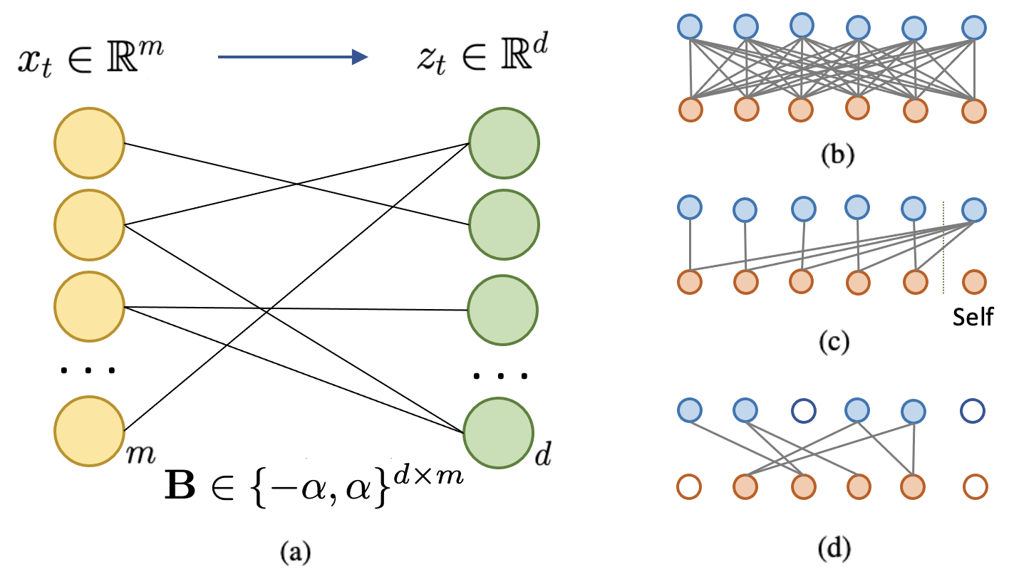
In this work, we extend the Lottery Ticket Hypothesis to time series Transformers, showing that we can prune and binarize the weights of the model and still maintain an accuracy similar to that of a Dense Transformer of the same structure. To achieve this, we employ the Biprop algorithm (Diffenderfer and Kailkhura, 2021), a state-of-the-art technique with proven success on complex datasets such as ImageNet (Deng et al., 2009). The combination of weight binarization and pruning is unique from previous efforts in Transformer compression. Moreover, each compression technique offers separate computational advantages: neural network pruning decreases the number of non-zero floating point operations (FLOPs), while binarization reduces the storage size of the model. The Biprop algorithm’s two compression methods rely on each other during the training process to identify a high-performing subnetwork within a randomly weighted neural network. The combination of pruning and weight binarization is depicted in Figure 1a.

We apply our approach to multivariate time series modeling. Research has shown that Transformers achieve strong results on time series tasks such as classification (Zerveas et al., 2021), anomaly detection (Xu et al., 2022; Tuli et al., 2022), and forecasting (Liu et al., 2021b; Zhou et al., 2021). Time series data is evident in systems such as IoT devices (Cook et al., 2019), engines (Malhotra et al., 2016), and spacecraft (Su et al., 2019; Baireddy et al., 2021), where new insights can be gleaned from the large amounts of unmonitored information. Moreover, such systems often suffer from resource constraints, making regular deep learning models unrealistic – for instance, in the Mars rover missions where battery-powered devices are searching for life (Bhardwaj and Gokhale, 2021). Other systems such as satellites contain thousands of telemetry channels that require granular monitoring. Deploying large deep learning models in each channel can be extremely inefficient. As a result, lightweight Transformer models have the potential to enhance a wide variety of applications.

In addition to pruning and binarizing the Transformer architecture, we simplify the complexity of the attention mechanism by applying two modifications. For anomaly detection and forecasting, which we model using overlapping sliding window inputs, we apply an attention mask to only consider attention at the current time step instead of considering attention for multiple previous time steps. For classification tasks, we apply a static mask to the query, key, and value projections, showing that only a subset of activations is needed in the attention module to achieve the same accuracy as that obtained using all the activations.

Finally, we estimate the computational savings of the model in terms of parameters, storage cost, and non-zero FLOPs, showing that pruned and binarized models achieve comparable accuracy to dense models with substantially lower computational costs.
Our contributions are as follows:

• We show that sparse and binary-weighted Transformers achieve comparable accuracy to Dense Transformers on three time series learning tasks (classification, anomaly detection, forecasting). To the best of our knowledge, this is the first research examining the efficacy of compressed neural networks on time series related learning.

• We examine pruning and binarization jointly in Transformer-based models, showing the benefits of each approach across multiple computational metrics. Weight binarization of Transformer based architectures has not been studied previously.

These findings provide new potential applications for the Transformer architecture, such as in resource-constrained environments that can benefit from time series related intelligence.

2. Related Work

In this section, we describe existing research related to Transformers in time series modeling, neural network pruning and compression, and finally efficient Transformer techniques.

2.1. Transformers in Time Series

Various works have applied Transformers to time series learning tasks (Wen et al., 2022). The main advantage of the Transformer architecture is the attention mechanism, which learns the pairwise similarity of input patterns. Moreover, it can efficiently model long-range dependencies compared to other deep learning frameworks such as LSTM’s (Liu et al., 2021b). Zerveas et al. (Zerveas et al., 2021) showed that we can use unsupervised pretrained Transformers for downstream time series learning tasks such as regression and classification. Additional work in time series classification has proposed using a “two tower” attention approach with channel-wise and time-step-wise attention (Liu et al., 2021a), while other work has highlighted the benefits of Transformers for satellite time series classification compared to both recurrent and convolutional neural networks (Rußwurm and Körner, 2020).

For anomaly detection tasks, Transformers have shown favorable results compared to traditional ML and deep learning techniques. Notably, Meng et al. (Meng et al., 2019) applied the model to NASA telemetry datasets and achieved strong accuracy (0.78 F1) in detecting anomalies. TranAD (Tuli et al., 2022) proposed an adversarial training procedure to exaggerate reconstruction errors in anomalies. Xu et al. (Xu et al., 2022) achieve state-of-the-art results in detecting anomalies in multivariate time series via association discrepancy. Their key finding is that anomalies have high association with adjacent time points and low associations with the whole series, accentuating anomalies.

Finally, Transformer variations have been proposed for time series forecasting to lower the attention complexity of long sequence time series (Li et al., 2019; Zhou et al., 2021; Liu et al., 2021b; Zhou et al., 2022), add stochasticity (Wu et al., 2020), and incorporate traditional time series learning methods (Zhou et al., 2022; Wu et al., 2021). Li et al. (Li et al., 2019) introduce LogSparse attention, which allows each cell to attend only to itself and its previous cells with an exponential step size. The Informer method (Zhou et al., 2021) selects dominant queries to use in the attention module based on a sparsity measurement. Pyraformer (Liu et al., 2021b) introduces a pyramidal attention mechanism for long-range time series, allowing for linear time and memory complexity. Wu et al. (Wu et al., 2020) use a Sparse Transformer as a generator in an encoder-decoder architecture for time series forecasting, using a discriminator to improve the prediction.

Figure 1. A sparse binary linear layer (left) and various attention modules (right). a) An example of a sparse and binary linear module, with binary weights $\mathbf{B}$ scaled to $\{-\alpha,\alpha\}$. b) A fully-connected attention module, where each point represents a time step ($w=6$). c) The Step-T attention module, where each past time point attends to itself and the latest time point $t$ attends to all past time points. d) An attention module with sparse Query (Q), Key (K), and Value (V) activations.

2.2. Compressed Neural Networks

Pruning unimportant weights from neural networks was first shown to be effective by Lecun et al. (LeCun et al., 1989). In recent years, deep learning has scaled the size and computational cost of neural networks. Naturally, research has been directed at decreasing size (Han et al., 2015) and energy consumption (Yang et al., 2017) of deep learning models.

The Lottery Ticket Hypothesis (Frankle and Carbin, 2019) showed that randomly initialized neural networks contain sparse subnetworks that, when trained in isolation, achieve comparable accuracy to a trained dense network of the same structure. The implications of this finding are that over-parameterized neural networks are no longer necessary, and we can prune large models and still maintain the original accuracy.

Subsequent work found that we do not need to train neural networks at all to find accurate sparse subnetworks; instead, we can find a high performance subnetwork using the randomly initialized weights (Ramanujan et al., 2020; Malach et al., 2020; Chijiwa et al., 2021; Gorbett and Whitley, 2023). Edge-Popup (Ramanujan et al., 2020) applied a scoring parameter to learn the importance of each weight, using the straight-through estimator (Bengio et al., 2013) to find a high accuracy mask over randomly initialized models. Diffenderfer and Kailkhuram (Diffenderfer and Kailkhura, 2021) introduced the Multi-Prize Lottery Ticket Hypothesis, showing that 1) multiple accurate subnetworks exist within randomly initialized neural networks, and 2) these subnetworks are robust to quantization, such as binarization of weights. In this work, we use the Biprop algorithm proposed in (Diffenderfer and Kailkhura, 2021) to binarize the weights of Transformer models.

2.3. Compressed and Efficient Transformers

Large-scale Transformers such as the BERT (110 million parameters) are a natural candidate for pruning and model compression (Tay et al., 2022; Ganesh et al., 2021). Chen et al. (Chen et al., 2021) first showed that the Lottery Ticket Hypothesis holds for BERT Networks, finding accurate subnetworks between 40% and 90% sparsity. Jaszczur et al. (Jaszczur et al., 2021) proposed scaling Transformers by using sparse variants for all layers in the Transformer. Other works have reported similar findings (Lepikhin et al., 2020; Fedus et al., 2021), showing that sparsity can help scale Transformer models to even larger levels.

Other works have proposed modifications for more efficient Transformers aside from pruning (Tay et al., 2022). Most research has focused on improving the $\mathcal{O}(n^{2})$ complexity of attention, via methods such as fixed patterns (Qiu et al., 2019), learnable patterns (Kitaev et al., 2020), low rank/kernel methods (Wang et al., 2020; Choromanski et al., 2020), and downsampling (Zhang et al., 2021; Beltagy et al., 2020). Various other methods have been proposed for compressing BERT networks such as pruning via post-training mask searches (Kwon et al., 2022), block pruning (Lagunas et al., 2021), and 8-bit quantization (Zafrir et al., 2019). We refer readers to Tay et al. (Tay et al., 2022) for details.

Despite the various works compressing Transformers, we were not able to find any research using both pruning and binarization. Utilizing both methods allows for more efficient computation (measured using FLOPs) as well as a significant decrease in storage (due to binary weights). Additionally, we find that our proposed model is still a fraction of the size of compressed NLP Transformers models when trained on time series tasks. For instance, TinyBERT (Jiao et al., 2020) contains 14.5 million parameters and 1.2 billion FLOPs, compared to our models which contain less than 1.5 million binary parameters and 38 million FLOPs.

3. Method

Our model consists of a Transformer encoder (Vaswani et al., 2017) with several modifications. We base our model off of Zerveas et al. (Zerveas et al., 2021), who propose using a common Transformer framework for several time series modeling tasks. To begin, we describe the base architecture of the Transformer as applied to multivariate time series. Subsequently, we describe the techniques used for pruning and binarization. Finally, we describe the two changes applied to the attention mechanism.

3.1. Dense Transformer

We denote fully trained Transformers with no pruning and floating point 32 (FP32) weights as Dense Transformers. Let $\mathbf{X_{t}}\in\mathbb{R}^{w\times m}$ be a model input for time $t$ with window size $w$ and $m$ features. Each input contains $w$ feature vectors $\mathbf{x}\in\mathbb{R}^{m}:\mathbf{X_{t}}\in\mathbb{R}^{w\times m}=[\mathbf{x_{t-w}},\mathbf{x_{t-w+1}},...,\mathbf{x_{t}}]$, ordered in time sequence of size $w$. In classification datasets $w$ is predefined at the sample or dataset level. For anomaly detection and forecasting tasks, we fix $w$ to 50 or 200 and use an overlapping sliding window as inputs.

The standard architecture (pre-binarization) projects $m$ features onto a $d$-dimensional vector space using a linear module with learnable weights $\mathbf{W_{p}}\in\mathbb{R}^{d\times m}$ and bias $\mathbf{b_{p}}\in\mathbb{R}^{d}$. We use the standard positional encoder proposed by Vaswani et al. (Vaswani et al., 2017), and we refer readers to the original work for details. For the Dense Transformer classification models, we use learnable positional encoder (Zerveas et al., 2021). Zerveas et al. (Zerveas et al., 2021) propose using batch normalization instead of layer normalization used in traditional Transformer NLP models. They argue that batch normalization mitigates the effects of outliers in time series data. We found that for classification tasks, batch normalization performed the best, while in forecasting tasks layer normalization worked better. For anomaly detection tasks we found that neither normalization technique was needed.

Each Transformer encoder layer consists of a multi-head attention module followed by ReLU layers. The self-attention module takes input $\mathbf{Z_{t}}\in\mathbb{R}^{w\times d}$ and projects it onto a Query ($\mathbf{Q}$), Key ($\mathbf{K}$), and Value ($\mathbf{V}$), each with learnable weights $\mathbf{W}\in\mathbb{R}^{d\times d}$ and bias $\mathbf{b}\in\mathbb{R}^{d}$. Attention is defined as $Attention(\mathbf{Q},\mathbf{K},\mathbf{V})=Softmax\left(\frac{\mathbf{Q}\mathbf{K}^{\intercal}}{\sqrt{d}}\right)\mathbf{V}$. Queries, keys, and values are projected by the number of heads ($h$) to create multi-head attention. The resultant output $\mathbf{Z_{t}}^{\prime}$ undergoes a nonlinearity before being passed to the next encoder layer. The Transformer consists of $N$ encoder layers followed by a final decoder layer. For classification tasks, the decoder outputs $l$ classification labels: $\mathbf{X^{\prime}_{t}}\in\mathbb{R}^{w\times l}$, which are averaged over $w$. For anomaly detection and forecasting, the decoder reconstructs the full input: $\mathbf{X^{\prime}_{t}}\in\mathbb{R}^{w\times m}$.

3.2. Sparse Binary Transformer

Central to our binarization architecture is the Biprop algorithm (Diffenderfer and Kailkhura, 2021), which uses randomly initialized floating point weights to find a binary mask over each layer. Given a neural network with weight matrix $\mathbf{W}\in\mathbb{R}^{i\times j}$ initialized with a standard method such as Kaiming Normal (He et al., 2015), we can express a subnetwork over neural network $f(x;\mathbf{W})$ as $f(x;\mathbf{W}\odot\mathbf{M})$, where $\mathbf{M}\in\{0,1\}$ is a binary mask and $\odot$ is an elementwise multiplication.

To find $\mathbf{M}$, parameter $\mathbf{S}\in\mathbb{R}^{i\times j}$ is initialized for each corresponding $\mathbf{W}\in\mathbb{R}^{i\times j}$. $\mathbf{S}$ acts as a score assigned to each weight dictating the importance of the weights contribution to a successful subnetwork. Using backpropagation as well as the straight-through estimator (Bengio et al., 2013), the algorithm takes pruning rate hyperparameter $p\in[0,1]$, and on the forward pass computes $\mathbf{M}_{k}$ at layer $m$ as

(1) $$\mathbf{M}_{k}=\begin{cases}1&\text{if $|\mathrm{S}_{k}|\in\{\tau(k)_{k=1}^{l_{m}}\geq[l_{m}p]\}$}\\ 0&\text{otherwise}\end{cases}$$

where $\tau$ sorts indices $\{k\}^{l}_{k=1}\in\mathrm{S}$ such that $|S_{\tau(k)}|\leq|S_{\tau(k+1)}|$. Masks are computed by taking the absolute value of scores for each layer, and setting the mask to 1 if the value falls above the top $p^{th}$ percentile.

To convert each layer to binary weights Biprop introduces gain term $\alpha\in\mathbb{R}$, which is common to Binary Neural Networks (BNN’s) (Qin et al., 2020). The gain term utilizes floating-point weights prior to binarization during training. During test-time, the alpha parameter scales the binarized weight vector. The parameter rescales binary weights $\mathbf{B}\in\{-1,1\}$ to $\{-\alpha,\alpha\}$, and the network function becomes $f(x;\alpha(\mathbf{B}\odot\mathbf{M}))$. $\alpha$ is calculated as

(2) $$\alpha=\frac{||\mathbf{M}\odot\mathbf{W}||_{1}}{||\mathbf{M}||_{1}}$$

with $\mathbf{M}$ being multiplied by $\alpha$ for gradient descent (the straight-through estimator is still used for backpropagation). This calculation was originally derived by Rastegari et al. (Rastegari et al., 2016).

In our approach we create sparse and binary modules for each linear and layer normalization layer. Our model consists of two linear layers at the top most level: one for projecting the initial input (embedding in NLP models) and one used for the decoder output. Additionally, each encoder layer consists of six linear layers: $\mathbf{Q}$, $\mathbf{K}$, and $\mathbf{V}$ projections, the multi-head attention output projection, and two additional layers to complement multi-head attention.

3.3. Attention Modifications

In this section we describe two modifications made to the attention module to reduce its quadratic complexity. Several previous works have proposed changes to attention in order to lessen this bottleneck, such as Sparse Transformers (Child et al., 2019), ProbSparse Attention (Zhou et al., 2021), and Pyramidal Attention (Liu et al., 2021b). While each of these works present quality enhancements to the memory bottleneck of attention, we instead seek to evaluate whether simple sparsification approaches can retain the accuracy of the model compared to canonical attention. Our primary motivation for the following attention modifications are to test whether a compressed Transformer can retain the same accuracy as a Dense Transformer.

3.3.1. Fixed Q,K, and V Projection Mask

To reduce the computational complexity of the matrix multiplications within the attention module, we apply random fixed masks to the $\mathbf{Q}$, $\mathbf{K}$, and $\mathbf{V}$ projections. We hypothesize that we can retain the accuracy of full attention by using this “naive” activation pruning approach, which requires no domain knowledge. We argue that the success of this approach provides insight into the necessity of full attention computations. In other words, Transformers are expressive and powerful enough for certain tasks that we can prune the models in an unsophisticated way and maintain accuracy. Moreover, many time series datasets and datasets generated at the edge are often times simplistic enough that we can apply this unsophisticated pruning (Gorbett et al., 2022a, b).

To apply this pruning, on model initialization we create random masks with prune rate $p_{a}\in\{0,1\}$ for each attention module and each projection Q,K, and V. Attention heads within the same module inherit identical Q, K, or V masks. The mask is applied to each projection during train and test. In each of our models we set the prune rate $p_{a}$ of the attention module equal to the prune rate of the linear modules ($p_{a}=p$).

3.3.2. Step-t Attention Mask

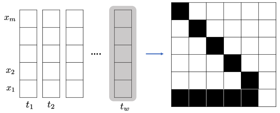
For anomaly detection and single-step forecasting tasks, the Sparse Binary Transformer (SBT) algorithm relies on reconstructing or predicting outputs at the current time step $t$ for each feature $m$, despite $w$ time steps of data being provided to the model. Specifically, the SBT model is only interested in input vector $\mathbf{x_{t}}\in\mathbb{R}^{m}$. For anomaly detection, the model reconstructs $\mathbf{x_{t}}$ from the input, while in forecasting tasks the model masks $\mathbf{x_{t}}=0$ prior to model input, reconstructs the actual values during training and inference.

In both tasks, vector $\mathbf{x_{t}}$ contains the only values necessary for the model to learn, and our loss function reflects this by only computing error for these values. As a result, computing attention for each other time step adds unnecessary computation. As depicted in Figure 2, we pass a static mask to the attention module to compute attention only at step-T. We additionally exclude attention computation at step-T with itself, forcing the variable to attend to historical time points for prediction. Finally, we add diagonal ones to the attention mask at all past time points to add stability to training. This masking method allows us to propagate the full input sample to multiple attention layers, helping us retain relevant historical information for downstream layers that would not be possible by changing the sizes of Q, K, and V to only model the $t$ time step.

Figure 2. Step-t Attention Mask Left: For the forecasting task we mask inputs during training in order to simulate unknown future time points. Right: The Step-T attention mask used to calculate attention only at the current time-step versus past values. Using this mask rather than setting our Query dimension to one enables us to pass time window vectors along multiple encoder layers.

4. Experiments

In this section we detail our experiments for time series classification, anomaly detection, and forecasting. Common to each learning task, we normalize each dataset prior to training such that each feature dimension $m$ has zero mean and unit variance. We use the Transformer Encoder as described in Section 3, training each learning task and dataset using the Dense Transformer and the SBT to compare accuracy. Finally, we run each experiment three times with a different weight seed, and present the average result. For the SBT model, varying the weight seed shows evidence of the robustness to hyperparameters. Specific modifications to the model are made for each learning task, which we describe in the following sections. Additional training and architecture details can be found in the Appendix.

4.1. Classification

For our first time series learning task we select several datasets from the UCR Time Series Classification Repository (Bagnall et al., 2017). The datasets contain diverse characteristics including varying training set size (204-30,000), number of features (13-200), and window size (30-405). We choose three datasets with the largest test set size (Insect Wingbeats, Spoken Arabic Digits, and Face Detection) as well as two smaller datasets (JapaneseVowels, Heartbeat). Each dataset contains a set window size except for Insect Wingbeats and Japanese Vowels, which contain a window size up to 30 and 29, respectively. In these datasets, we pad samples with smaller windows to give them consistent window sizes. The decoder in our classification architecture is a classification head, rather than a full reconstruction of the input as is used in anomaly detection and forecasting tasks. The SBT classification model is trained and tested using the fixed Q,K,V projection mask as described in Section 3.3.

Results In Table 1, we show that SBT s perform as well as, or similar to, the Dense Transformer for each dataset at $p=0.5$ and $p=0.75$. Our models are averaged over three runs with different weight seeds. When comparing our model to state-of-the-art approaches, we find that the SBT achieves strong results across each dataset, with the highest reported performance on three out of the five datasets. Further, the SBT models perform consistently across datasets while models such as Rocket (Dempster et al., 2020) and Fran et al. (Franceschi et al., 2019) have lower performance on one or more datasets.

Surprisingly, the SBT model achieves stronger average accuracy than the Dense Transformer (80.2% versus 78.8%), indicating that the pruned and binarized Transformer achieves a robust performance across datasets. Despite this, Insect Wingbeats and Japanese Vowels datasets achieved a slightly lower performance at $p=0.5$ with a more substantial dropoff at $p=0.75$, indicating the model may lose some of its power on certain tasks.

Model	Arabic Digits	Heart Beat	Insect W.B.	Japan. Vowels	Face Detect.	Mean
XGBoost	69.6	73.2	36.9	96.2	63.3	67.8
LSTM	31.9	72.2	17.6	79.7	57.7	51.8
Rocket (Dempster et al., 2020)	71.2	75.6	-	86.5	64.7	74.5
Fran et al. (Franceschi et al., 2019)	95.6	75.6	16.0	98.9	52.8	67.8
DTW_D	96.3	71.7	-	94.9	52.9	79.0
Dense Trans.	98.0	76.6	63.4	98.0	56.0	78.8
$SBT_{p=0.5}$	98.2	77.2	64.1	95.3	66.1	80.2
$SBT_{p=0.75}$	98.6	78.5	61.3	85.3	65.8	77.9

Table 1. Accuracy of time series classification models on five datasets. Results are obtained from (Zerveas et al., 2021; Franceschi et al., 2019). SBT models achieve higher accuracy than prior works (excluding the Dense Transformer) in each case, except for the Japanese Vowels dataset. Additionally, SBT models achieve accuracy within 2.7% of the Dense Transformer for each dataset.

4.2. Anomaly Detection

For the anomaly detection task we test the SBT algorithm on established multivariate time series anomaly detection datasets used in previous literature: Soil Moisture Active Passive Satellite (SMAP) (Hundman et al., 2018), Mars Science Labratory rover (MSL) (Hundman et al., 2018), and the Server Machine Dataset (SMD) (Su et al., 2019). SMAP and MSL contain telemetry data such as radiation and temperature, while SMD logs computer server data such as CPU load and memory usage. The datasets contain benign samples in the training set, while the test set contains labeled anomalies (either sequences of anomalies or single point anomalies).

Our model takes sliding window data as input and reconstructs data at $\mathbf{x_{t}}$ given previous time points. We use MSE to reconstruct each feature in $\mathbf{x_{t}}$. We use the step-T attention mask as described in Section 3. To evaluate our results, we adopt an adjustment strategy similar to previous works (Xu et al., 2022; Su et al., 2019; Shen et al., 2020; Tuli et al., 2022): if any anomaly is detected within a successive abnormal segment of time, we consider all anomalies in this segment to have been detected. The justification is that detecting any anomaly in a time segment will cause an alert in real-world applications.

To flag anomalies, we retrieve reconstruction loss $\mathbf{x^{\prime}_{t}}$ and threshold $\tau$, and consider anomalies where $\mathbf{x^{\prime}_{t}}>\tau$. Since our model is trained with benign samples, anomalous samples in the test set should yield a higher $\mathbf{x^{\prime}_{t}}$. We compute $\tau$ using two methods from previous works: A manual threshold (Xu et al., 2022) and the Peak Over Threshold (POT) method (Siffer et al., 2017). For the manual threshold, we consider proportion $r$ of the validation set as anomalous. For SMD $r=0.5\%$, and for MSL and SMAP $r=1\%$. For the POT method, similar to OmniAnomaly (Su et al., 2019) and TranAd (Tuli et al., 2022), we use the automatic threshold selector to find $\tau$. Specifically, given our training and validation set reconstruction losses, we use POT to fit the tail portion of a probability distribution using the generalized Pareto Distribution. POT is advantageous when little information is known about a scenario, such as in datasets with an unknown number of anomalies.

Dataset	Metric	Manual Threshold		POT Threshold
		Dense	$\lx@glossaries@gls@link{acronym}{sbt}{\leavevmode SBT}_{p=0.75}$	Dense	$\lx@glossaries@gls@link{acronym}{sbt}{\leavevmode SBT}_{p=0.75}$
MSL	P	92.7	96.8	85.5	82.9
	R	100	100	100	100
	F1	96.2	96.8	92.1	91.1
SMD	P	85.4	85.3	99.9	100
	R	100	100	100	100
	F1	92.1	92.1	100	99.9
SMAP	P	93.9	93.7	85.9	84.9
	R	100	100	100	100
	F1	96.9	96.8	92.4	91.8

Table 2. Anomaly detection results with benign sample windows. We evaluate Precision (P), Recall (R), and the F1 score using both manual threshold and POT threshold technique. We find that the single time step prediction window achieves high accuracy when each past time-step in $w$ is benign. $w=200$ for SMD and $w=50$ for SMAP and MSL. These results indicate that when given time to stabilize after an anomalous event, our SBT framework can detect new anomalies with high accuracy. We evaluate our results using a manual threshold ($\tau$=0.5% for SMD, 1% for others) and the POT automatic threshold selector.

Results In Table 2 we report the unique findings of our single-step anomaly detection method using Precision, Recall, and F1-scores. Specifically, we find that when only considering inputs with fully benign examples in window $w$, both the SBT and the Dense Transformer achieve high accuracy on all three datasets (F1 between 90.6 and 100). In other words, we find that our model performance is best when we filter examples that have an anomalous sequence or data point in $[\mathbf{x_{t-w}},\mathbf{x_{t-w+1}},...,\mathbf{x_{t-1}}]$. For SMD, $w=200$ and for SMAP and MSL $w=50$. This observation implies that the model needs time to stabilize after an anomalous period. Intuitively, if an anomaly occurred recently, new benign observations will have a higher reconstruction loss as a result of their difference with the anomalous examples in their input window. We argue that this validation metric is logical in real-world scenarios, where monitoring of a system after an anomalous period of time is necessary.

We additionally report F1-scores compared to state-of-the-art time series anomaly detection models in Table 3. To accurately compare our model against existing methods, we use the full test set without filtering out benign inputs with anomalies in the near past. SBT results are much more modest, with F1-scores between 70 and 88. Despite this, our method still performs stronger than non-temporal algorithms such as the Isolation Forest, as well as other deep-learning based approaches such as Deep-SVDD and BeatGan.

Model	SMD	MSL	SMAP	Avg.
LOF	46.7	61.2	57.6	55.2
IsolationForest	53.6	66.5	55.5	58.5
OCSVM	56.2	70.8	56.3	61.1
DAGMM	57.3	74.6	68.5	66.8
VAR	74.1	77.9	64.8	72.3
MMPCACD	75.0	70.0	81.7	75.6
ITAD	79.5	76.1	73.9	76.5
Deep-SVDD	79.1	83.6	69.0	77.2
$\textbf{\lx@glossaries@gls@link{acronym}{sbt}{\leavevmode SBT}}_{p=0.9}$	82.5	78.5	70.6	77.2
CL-MPPCA	79.1	80.4	72.9	77.5
BeatGAN	78.1	87.5	69.6	78.4
$\textbf{\lx@glossaries@gls@link{acronym}{sbt}{\leavevmode SBT}}_{p=0.5}$	87	78.4	69.8	78.4
$\textbf{\lx@glossaries@gls@link{acronym}{sbt}{\leavevmode SBT}}_{p=0.75}$	88.0	79.3	70.6	79.3
LSTM-VAE	82.3	82.6	78.1	81.0
OmniAnomaly	85.2	87.7	86.9	86.6
Anomaly Transformer	92.3	93.6	96.7	94.2

Table 3. F1 scores of various time series anomaly detection models. We compare our SBT framework with several state-of-the-art algorithms on the anomaly detection task. The table is ordered by average F1 accuracy across each dataset. We evaluate our algorithm using the traditional method (different from Table 2), where each sample can contain anomalous events in its input window. We use a manual threshold to report results for the SBT model.

Model	ECL		Weather		ETTm1
	MSE	MAE	MSE	MAE	MSE	MAE
Informer	0.185	0.301	0.159	0.197	0.051	0.150
Pyraformer	0.149	0.305	-	-	0.081	0.214
Dense Trans.	0.182	0.299	0.173	0.225	0.070	0.201
$\lx@glossaries@gls@link{acronym}{sbt}{\leavevmode SBT}_{p=0.5}$	0.198	0.316	0.166	0.216	0.059	0.171
$\lx@glossaries@gls@link{acronym}{sbt}{\leavevmode SBT}_{p=0.75}$	0.221	0.333	0.168	0.218	0.070	0.191

Table 4. A summary of time series forecasting models on three datasets. Each SBT model is run three times with different weight seeds and averaged. Standard deviation is less than 0.01.

4.3. Forecasting

We test our method on single-step forecasting using the Step-T attention mask. Specifically, using the framework outlined by Zerveas et al. (Zerveas et al., 2021), we train our model by masking the input at the forecasting time-step $t$. For example, input $\mathbf{X_{t}}$ containing $m$ features and $t$ time-steps $[\mathbf{x_{t-w}},\mathbf{x_{t-w+1}},...,\mathbf{x_{t}}]$ is passed through the network with $\mathbf{x_{t}}=0$. We then reconstruct this masked input with the Transformer model, using mean squared error between the masked inputs reconstruction and the actual value. The masking method simulates unseen future data points during train time, making it compatible with the forecasting task during deployment.

We test our model on three datasets used in previous works: ECL contains electricity consumption of 321 clients in Kwh. The dataset is converted to hourly consumption values due to missing data. Weather contains data for twelve hourly climate features for 1,600 location in the U.S. ETTm1 (Electricity Transformer Temperature) contains 15-minute interval data including oil temperature and six additional power load features. Additional training details are available in the Appendix.

We compare our method against the Informer (Zhou et al., 2021) and the Pyra-former (Liu et al., 2021b) trained with single-step forecasting. Both are current state-of-the-art models that have shown robust results compared against a variety of forecasting techniques. Importantly, each method is compatible with multivariate time series forecasting as opposed to some research. We note that these models are built primarily for long-term time series forecasting (LSTF), which we do not cover in this work.

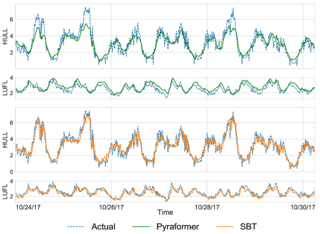
Results We evaluate results in Table 4 using MSE and MAE on the test set of each dataset. Results indicate that the SBT model achieves accuracy comparable to the Dense architecture in each dataset at $p=0.5$. Interestingly, the Weather at ETTm1 SBT models achieved better accuracy than the dense model at $p=0.5$. Both models additionally showed robustness to higher prune rates, with accuracy dropping off slowly. ECL on the other hand showed some sensitivity to prune rate, with a slight drop off when increasing the prune rate. We find that datasets with a higher dimensionality performed the worst: ECL contains 321 features, while Insect Wingbeats contains 200. Increasing the dimensionality of the model ($d$) mitigated some of these effects, however it was at the cost of model size and complexity. Despite this, we find that the SBT model is able to predict the general trend of complex patterns in data, as depicted in Figure 3.

Compared to state-of-the-art approaches such as the Pyraformer and Informer architectures, our general purpose forecasting approach performs comparably, or slightly worse, on the single-step forecasting task. Metrics were not substantially different for any of the models except for the ECL dataset, where Pyraformer was easily the best model. Comparing the architectures, we find that the SBT model achieves substantially lower computational cost than both the Informer and Pyraformer models. For example, on the ECL dataset, Pyraformer contains 4.7 million parameters and the Informer 12.7 million parameters (both FP32, while the SBT model contains 1.5 million binary parameters.

Figure 3. Time series predictions on the ETTm1 dataset for the Pyraformer (top) and Sparse Binary Transformer (bottom) . We show 600 predictions across each model for two features (HULL, LUFL).

4.4. Architecture

Each model in our framework consists of 2 encoder layers each with a multi-head attention module containing two heads. The feedforward dimensionality for each model is 256 with ReLU used for nonlinearity. Classification models had the best results using Batch Normalization layers, similar to (Zerveas et al., 2021), while forecasting models used Layer Normalization typical of other Transformer models. For anomaly detection we did not use Batch or Layer Normalization. For the output of our models, anomaly detection and forecasting rely on a single decoder linear layer which reconstructs the output to size ($m$, $w$), while classification outputs size ($d$, $num.classes$) and takes the mean of $d$ to formulate a final classification prediction. Further details are included in the Appendix and the code repository.

5. Computational Savings

In this section we estimate the computational savings achieved by using the SBT model. We will begin by introducing the metrics used to estimate computational savings, and will then summarize the results of these metrics for each model and task.

We note that several works (highlighted in Section 2) have proposed modifications to the Transformer in order to make attention more efficient. In this section, we concentrate on the enhancements achieved by 1) creating a sparsely connected Transformer with binary weights, and 2) simplifying the attention module for time series specific tasks such as single-step prediction and classification. We argue that these enhancements are independent of the achievements made by previous works.

5.1. Metrics

FLOPs (Non-zero). In the field of network pruning, FLOPs, or the number of multiply-adds, is a commonly used metric to quantify the efficiency of a neural network (Blalock et al., 2020). The metric computes the number of floating point operations required for an input to pass through a neural network. We use the ShrinkBench tool to calculate FLOPs, a framework proposed by Blalock et al. (Blalock et al., 2020) to perform standardized evaluation on pruned neural networks.

Our Transformer architecture contains FP32 activations at each layer along with binary weights scaled to $\{-\alpha,\alpha\}$. As a result, no binary operations are performed, and our total FLOPs count is a function of prune rate $p$. For example, a linear module with a standard FLOPs count of $d\times m$ has a new FLOPs count of $d\times m\times p$, where $p\in[0,1]$. Linear layers outside of attention do not need window size added to the matrix multiply because the inputs are permuted such that batch size is the second dimension of the layer input. Each equation counts the number of nonzero multiply-adds necessary for the neural network.

Attention Type	Q,K,V Proj.	$\mathbf{Q}\mathbf{V}^{\intercal}$	$\mathbf{AV}$
Canonical	$d^{2}w$	$d^{\prime}w^{2}$	$d^{\prime}w^{2}$
Step-T Mask	$(d^{2}w)p_{a}$	$(w-1)d^{\prime}$	$2(w-1)d^{\prime}$
Q,K,V Mask	$(d^{2}w)p_{a}$	$d^{\prime}(wp_{a})^{2}$	$(d^{\prime}w^{2})p_{a}$

Table 5. Non-zero FLOPs equations for various attention modules. These calculations assume $\mathbf{Q},\mathbf{K}$ and $\mathbf{V}$ are equal sized projections in $\mathbb{R}^{w\times d}$, and $d^{\prime}=d/h$. $\mathbf{Q}\mathbf{V}^{\intercal}$ and $\mathbf{AV}$ are additionally multiplied by $h$. $\mathbf{Q}$-scaling and softmax FLOPs excluded from this table.

					Dense Transformer			Sparse Binary Transformer				$\sim$Savings
Type	Dataset	$m$	$w$	$d$	Params (FP32) (K)	Size (Bits) (Mil.)	FLOPs (Mil.)	$p$	Params (Binary) (K)	Size (Bits) (Mil.)	FLOPs (Mil.)	Size (Bits) ($\frac{\text{Dense}}{\text{\lx@glossaries@gls@link{acronym}{sbt}{\leavevmode SBT}}}$)	FLOPs ($\frac{\text{Dense}}{\text{\lx@glossaries@gls@link{acronym}{sbt}{\leavevmode SBT}}}$)
Classification	Heartbeat	61	405	64	169.6	5.4	52.7	0.5	102.3	0.1	21.6	$\times$49.1	$\times$2.4
	Insect W.B.	200	30	128	555.5	17.8	5.4	0.5	420.1	0.4	2.7	$\times$40.0	$\times$2.0
	Arabic Dig.	13	93	64	167.1	5.3	2.8	0.5	100.0	0.1	1.3	$\times$49.5	$\times$2.2
	Japan.Vowels	12	29	32	75.5	2.4	0.3	0.5	41.6	0.04	0.2	$\times$52.9	$\times$2.1
	FaceDetection	144	62	128	414.9	13.3	8.3	0.5	281.3	0.3	4.0	$\times$44.7	$\times$2.1
Anomaly Detection	MSL	55	50	110	223.7	7.2	4.9	0.75	221.5	0.2	1.0	$\times$32.3	$\times$5.0
	SMAP	25	50	50	75.2	2.4	1.3	0.75	73.7	0.1	0.2	$\times$32.6	$\times$6.1
	SMD	38	200	76	132.8	4.2	19.5	0.75	129.8	0.1	1.9	$\times$32.7	$\times$10.5
Forecast.	ECL	321	200	350	1569.4	50.2	204.8	0.75	1563.9	1.6	74.5	$\times$32.1	$\times$2.7
	Weather	7	200	100	188.0	6.0	28.5	0.5	185.6	0.2	6.2	$\times$32.4	$\times$4.6
	ETTm1	12	200	64	102.0	3.3	15.5	0.5	100.0	0.1	2.6	$\times$32.6	$\times$5.9

Table 6. Computational savings for Dense Transformers compared to SBTs. SBT models achieve a substantial reduction in size and FLOPs count across all models. We denote parameters in thousands and size and FLOPs in millions, with savings calculated by dividing the Dense values by the SBT values.

Furthermore, we modify the FLOPs for the attention module to account for step-t attention mask and the fixed $\mathbf{Q},\mathbf{K},\mathbf{V}$ mask, as summarized in Table 5. In the standard attention module where $\mathbf{Q},\mathbf{K}$ and $\mathbf{V}$ are equal sized projections, matrix multiply operations ($\mathbf{Q}\mathbf{V}^{\intercal}$, $\mathbf{AV}$) for each head equate to $d^{\prime}w^{2}$, where $d^{\prime}=d/h$. For step-t attention, we only require computation at the current time step (the last row in Figure 2), while each each of the identities for past time steps equates to one. $\mathbf{A}\mathbf{V}$ requires double the computations because $\mathbf{V}$ contains FP32 activations multiplied by the diagonal in $\mathbf{A}$. For the fixed mask, since $\mathbf{Q}$ and $\mathbf{K}$ are sparse projections, we only require $(wp_{a})^{2}$ nonzero computations in the matrix multiply. Since $\mathbf{A}$ is a dense matrix, we require $w^{2}$ FLOPs to multiply sparse matrix $\mathbf{V}$.

A simplified equation for network FLOPs becomes $2L+N(2L+MHA)$, where $L$ is a linear layer, $N$ is the number of attention layers, and $MHA$ is the multihead attention FLOPs (details described in Table 5). Several FLOP counts are omitted from this equation, which we include in our code, including positional encoding, $Q$-scaling, and layer and batch norm.

Storage Size. We measure the size of each model in total bits. Standard networks rely on weights optimized with the FP32 data type (32 bits). We consider each binarized module in our architecture to contain single bit weights with a single FP32 $\alpha$ parameter for each layer. Anomaly detection and classification datasets contain 14 binarized modules, and forecasting contains 18 with the additional binarization of the layer normalization. We note that the binarized quantities are only theoretical as a result of the PyTorch framework not supporting the binary data type. Hardware limitations are also reported in other works (Frankle and Carbin, 2019).

5.2. Model Size Selection

Important to our work is tuning the size of each model. We analyze whether we can create a Dense Transformer with a smaller number of parameters and still retain a performance on par with a larger model. Our motivation for model size selection is two-fold: 1) Previous research has found that neural networks need to be sufficiently overparameterized to be pruned and retain the same accuracy of the dense model and 2) The time series datasets studied in this paper have a smaller number of dimensions than the vision datasets studied in most pruning and model compression papers. The effect of model overparameterization is that we need a dense model with enough initial parameters in order to prune it and still retain high performance. Theoretical estimates on the number of required parameters are proposed by the Strong Lottery Ticket Hypothesis (Pensia et al., 2020; Orseau et al., 2020) and are further explored in other pruning papers (Diffenderfer and Kailkhura, 2021; Chijiwa et al., 2021). On the other hand, the limited features of some time series datasets (such as Weather with 7 features) leads us to wonder whether we could simply create a smaller model.

To alter the model size, we vary the embedding dimension $d$ of the model. To find the ideal size of the model, we start from a small embedding dimension (such as 8 or 16), and increase the value in the Dense Transformer until the model performance on the validation set stops increasing. With this value of $d$, we test the SBT model.

Our results show that in each dataset, Dense Transformers with a smaller embedding dimension $d$ either a) perform worse than the SBT at the optimized size, b) contain more parameters (as measured in total bits), c) have more FLOPs, or d) some combination of the above. In almost every dataset, the smaller Dense Transformer performs worse than the SBT while also requiring more size and FLOPs. The exception to this was Spoken Arabic Digits, where the smaller Dense Transformers ($d=16$ and $d=32$) performed slightly better than the SBT with $d=64$. Additionally, these models had a lower FLOPs count. The advantage of the SBT model in this scenario was a substantially lower storage cost than both smaller Dense models. Even if both Dense Transformer models were able to be quantized to 8-bit weights, the storage of the SBT would still be many times lower. The ETTm1 dataset additionally had high performance Dense Transformers with a smaller size ($d=16,d=32)$. However, both models were substantially more costly in terms of storage and additionally had a higher FLOPs count. Detailed results are provided in the Appendix.

5.3. Analysis

Results in Table 6 highlight the large computational savings achieved by SBT. We find that layer pruning reduces FLOPs count (due to the added nonzero computations), while binarization helps with the storage size.

Notably, all models have a FLOPs count at least two times less than the original Dense model. FLOPs are dramatically reduced in the anomaly detection and forecasting datasets, largely due to the step-t masking. Classification datasets have a dense attention matrix, leading to a smaller FLOPs reduction due to the softmax operation and the $AV$ calculation (where $V$ is sparse). We note that using a higher prune rate can reduce the FLOPs more, however we include results at 50% prune rate for classification since these models achieved slightly better accuracy.

We highlight the storage savings of SBT models by measuring bit size and parameter count. Table 6 summarizes the substantial reduction in bit size for every model, with only two SBT models having a bit size greater than 1 million (Insect Wingbeats and ECL). The two models with a larger size also had the highest dimensionality $m$, and consequently $d$.

We note that SBT models contain a small number of FP32 values due to the single $\alpha$ parameter in each module. Additionally, we forego a learnable encoding layer in SBT classification models, leading to a smaller overall count. Finally, no bias term is added to the SBT modules, leading to a smaller number of overall parameters.

Compared to other efficient models, our model generally has a lower FLOPs count. For example, MobileV2 (Sandler et al., 2018) has 16.4 million FLOPs when modeling CIFAR10, while EfficientNetV2 (Tan and Le, 2021) has 18.1 million parameters.

6. Discussion

We show that Sparse Binary Transformers attain similar accuracy to the Dense Transformer across three multivariate time series learning tasks: anomaly detection, forecasting, and classification. We estimate the computational savings of SBT’s by counting FLOPs as well as total size of the model.

6.1. Applications

SBT s retain high performance compared to dense models, coupled with a large reduction in computational cost. As a result, SBT s have the potential to impact a variety of new domains. For example, sensors and small embedded systems such as IoT devices could employ SBT s for intelligent and data-driven decisions, such as detecting a malicious actor or forecasting a weather event. Such devices could be extended into new areas of research such as environmental monitoring. Other small capacity applications include implantable devices, healthcare monitoring, and various industrial applications.

Finally, lightweight deep learning models can also benefit larger endeavors. For example, space and satellite applications, such as in the MSL and SMAP telemetry datasets, collect massive amounts of data that is difficult to monitor. Employing effective and intelligent algorithms such as the Transformer could help in the processing and auditing of such systems.

6.2. Limitations and Future Work

Although SBT s theoretically reduce computational costs, the method is not optimized for modern libraries and hardware. Python libraries do not binarize weights to single bits, but 8-bit counts. Special hardware in IoT devices and satellites could additionally make implementation a burden. Additionally, while our implementation shows that sparse binarized Transformers exist, the Biprop algorithm requires backpropagation over a dense network with randomly initialized FP32 weights. Hence, finding accurate binary subnetworks requires more computational power during training than it does during deployment. This may be a key limitation in devices seeking autonomy. In addition to addressing these limitations, a logical step for future work would be to implement SBT s in state-of-the-art Transformer models such as the Pyramformer for forecasting and the Anomaly Transformer for time series anomaly detection.

SBT s have the potential to enable widespread use of AI across new applications. The Transformer stands as one of most powerful deep learning models in use today, and expanding this architecture into new domains provides promising directions for the future.

7. Acknowledgements

This work was supported in part by funding from NSF under Award Numbers ATD 2123761, CNS 1822118, NIST, ARL, Statnett, AMI, NewPush, and Cyber Risk Research.

Supplemental Materials

Appendix A Ablation Studies

We conduct two ablation studies testing the effects of removing the individual pruning mechanisms from the attention computation. We note that the attention pruning methods complement Biprop – Biprop mainly reduces the model size, whereas attention pruning does a better job at reducing the FLOPs. Each ablation experiment is averaged over three experimental runs with different seeds.

Table 1 highlights the effects of removing random pruning from the time series classification models. Notably, Biprop plus random pruning performs comparably to, or better than, Biprop on its own. Adding random pruning even outperforms using only Biprop with the Japanese Vowels dataset.

Table 2 highlights the results of attention variations for both anomaly detection and forecasting tasks. Specifically, we look at our proposed approach (Biprop+Step-T Mask), Biprop plus an identity matrix mask in the attention layers, and finally Biprop only. We report results using mean squared error (MSE) loss averaged over three runs.

Results show that Biprop plus the Step-T mask performs comparably to using Biprop only. For anomaly detection tasks, the MSE is even lower compared to just using Biprop. Comparing both methods to the Biprop plus the identity matrix attention mask, we can see a significant difference in the results: the identity matrix attention mask attains a higher loss in each case.

Dataset	Biprop+Random Pruning	Biprop
Arabic Digits	98.2	98.2
Heartbeat	77.7	77.1
Insect Wingbeats	64.1	64
Japanese Vowels	95.3	84.4
Face Detection	66.1	65.9

Table 1. We compare Biprop with Biprop plus random pruning on classification tasks. We find that random pruning of the attention activations does not hurt classifcation accuracy, and in fact helps it in the case of the Japanese Vowels dataset.

Dataset	Biprop+ Step-T	Biprop+ Identity Matrix	Biprop Only
Anomaly Detection
MSL	0.277	0.364	0.357
SMAP	0.117	0.131	0.125
SMD	0.037	0.041	0.052
Forecasting
ETTm1	0.059	0.068	0.070
ECL	0.198	0.204	0.182
Weather	0.166	0.180	0.166

Table 2. We compare Biprop plus the Step-T attention mask with two other methods. We find that Biprop with the Step-T mask performs similarly to using Biprop with full attention (Biprop Only). Biprop with an Identity Mask on the attention computation performs worse than the other two methods. We report results using MSE loss averaged across three runs.

Appendix B Training Details

Each model is trained with Adam optimization with a learning rate of 1e-3 except for InsectWingbeats, where we use a learning rate of 1e-4. For Dense Transformer classification models we use a learnable positional encoding, while in all other models we use a standard positional encoding.

We found that SBT models sometimes take slightly longer to converge, hence we train the models for more epochs in the forecasting and classification tasks. These numbers are specified in the configuration files in the code repository. Batch Normalization is used for classification tasks, layer normalization is used for forecasting tasks, and no normalization is used for anomaly detection.

Appendix C Analysis

C.1. Attention Magnitude Pruning versus Random Pruning

As apart of our attention pruning analysis, we also applied magnitude pruning to the attention layers. However, this method requires extra computation as a result of the sorting required to take the top activation’s for each input. Below we compare the results of magnitude pruning versus random pruning, finding that random pruning achieves similar accuracy to magnitude pruning at a lower computational cost.

Dataset	Mag. Prune	Rand. Prune
Arabic	98.2	98.2
Heartbeat	77.2	77.7
Insect	64.4	64.1
Japanese	94.9	95.3
Face Det.	66.3	66.1

Table 3. Random pruning versus activation magnitude pruning. We find that random pruning achieves similar accuracy to magnitude pruning with lower computational cost.

C.2. Model size savings of Biprop versus Pruning

In Table 4 we compare the model size savings of Biprop compared to 32-bit pruning as well as pruning plus quantization (8-bit). We show that, even compared to pruning plus 8-bit quantization, Biprop achieves substantially lower model size.

Dataset	Bin.	Prune	Pruning+ Quantization
Classification
Heartbeat	$\times$ 49.10	$\times$3.2	$\times$11.7
Insect	$\times$ 39.98	$\times$ 2.6	$\times$ 9.4
Arabic	$\times$ 49.51	$\times$ 3.2	$\times$ 11.8
Japanese	$\times$ 52.85	$\times$ 3.5	$\times$ 12.8
FaceDet.	$\times$ 44.67	$\times$ 2.8	$\times$ 10.5
Anomaly Detection
MSL	$\times$ 32.31	$\times$ 3.7	$\times$ 11.8
SMAP	$\times$ 32.65	$\times$ 3.7	$\times$ 11.9
SMD	$\times$ 32.74	$\times$ 3.7	$\times$ 11.9
Forecasting
Electricity	$\times$ 32.11	$\times$ 3.7	$\times$ 11.7
Weather	$\times$ 32.42	$\times$ 2.0	$\times$ 7.2
ETTm1	$\times$ 32.65	$\times$ 2.0	$\times$ 7.3

Table 4. Comparison of the size between Biprop, 32-bit pruning, and 32-bit pruning + quantization. Biprop achieves the greatest model size compression by a large degree.

Appendix D Dataset Details

We report the details of datasets used for each task below. For anomaly detection and forecasting tasks, we set the window size $w$ to a fixed value, while in classification, $w$ is predefined.

Dataset	Train Size	Test Size	$m$	$w$	Classes
Arabic	6,599	2,199	13	93	10
Heartbeat	204	205	61	405	2
Insect	30k	20k	200	30	10
Japanese	270	370	12	29	9
Face Det.	5,890	3,524	144	62	2

Table 5. A summary of classification datasets.

Dataset	Train Size	Test Size	Features($m$)	Length ($w$)
ECL	23,377	2,928	321	200
Weather	28,005	7,060	12	200
ETTm1	45,697	11,904	7	200

Table 6. A summary of forecasting datasets.

Dataset	Train Size	Test Size	Features($m$)	Length ($w$)
SMAP	135,183	427,617	25	50
MSL	58,317	73,729	55	50
SMD	708,405	708,420	38	200

Table 7. A summary of anomaly detection datasets.

Appendix E Model Size Selection

We measure model performance as well as computational cost at varying sizes for each model. To vary the size, we increase the embedding dimension $d$ for each model and dataset combination. Tables 8 and 9 show the results for each model size and dataset combination. Overall, we find that the SBT generally performs better than the smaller Dense Transformer in terms of performance, except in a few cases. In all scenarios, the SBT model has at least one computational advantage in terms of storage size or FLOPs count.

Additionally we find that, common with our intuition, datasets with a higher dimensionality $m$ need a higher embedding dimension, while simpler datasets are successful with a smaller embedding dimension. For example, Insect Wingbeats ($m=200$), Face Detection ($m=144$), and ECL ($m=321$) require $d\geq 128$ to achieve optimal performance.

			Dense Transformer			Sparse Binary Transformer
Dataset	$m$ (Num. Features)	$d$	Accuracy	Params (FP32) (K)	FLOPs (Mil.)	Accuracy	Params (Binary) (K)	FLOPs (Mil.)
Heartbeat	61	64	76.6	169.6	52.73	77.2	102.3	21.57
		16	28.8	36.6	11.81	72.2	19.5	4.95
		32	71.1	76.9	24.20	74.5	43.1	9.87
		128	75.6	404.2	124.73	75.1	270.7	52.45
Insect Wingbeats	200	128	63.4	555.5	5.42	64.1	420.9	2.67
		256	65.2	1,503.5	19.77	64.4	1,234.9	9.80
		64	57.9	229.0	1.60	51.4	161.3	0.79
		400	64.9	3,040.0	46.60	64.6	2,620.8	23.16
Japanese Vowels	12	32	98.0	75.5	0.33	95.3	41.6	0.16
		8	92.5	17.7	0.05	78.5	8.9	0.02
		16	93.6	36.0	0.12	87.7	18.8	0.06
		64	96.2	166.9	1.01	94.1	99.9	0.49

Table 8. Classification Model size selection: Performance of various sized models on each classification dataset. We include the parameter count as well as FLOPs for both the dense and sparse binary Transformer models. Parameters are floating-point 32 in the Dense Transformer and Binary in the SBT.

			Dense Transformer			Sparse Binary Transformer
Dataset	$m$ (Num. Features)	$d$	MSE	Params (FP32) (K)	FLOPs (Mil.)	MSE	Params (Binary) (K)	FLOPs (Mil.)
ECL	321	350	0.178	1,569.4	204.76	0.187	1,569.4	74.54
		128	0.199	348.2	40.83	0.337	345.1	10.18
		256	0.197	956.0	120.88	0.27	951.6	40.06
		400	0.216	1,953.2	258.03	0.191	1,947.2	97.21
Weather	7	100	0.173	188.0	28.50	0.166	185.6	6.24
		32	0.171	44.2	6.61	0.187	42.5	0.69
		64	0.172	102.7	15.53	0.177	100.6	2.61
		128	0.169	268.7	40.75	0.166	266.0	10.14

Table 9. Forecasting Model size selection: Performance of various sized models on each forecasting dataset. We include the parameter count as well as FLOPs for both the dense and sparse binary Transformer models. Parameters are floating-point 32 in the Dense Transformer and Binary in the SBT.

References

- (1)
- Bagnall et al. (2017) A. Bagnall, J. Lines, A. Bostrom, J. Large, and E. Keogh. 2017. The Great Time Series Classification Bake Off: a Review and Experimental Evaluation of Recent Algorithmic Advances. Data Mining and Knowledge Discovery 31 (2017), 606–660. Issue 3.
- Baireddy et al. (2021) Sriram Baireddy, Sundip R Desai, James L Mathieson, Richard H Foster, Moses W Chan, Mary L Comer, and Edward J Delp. 2021. Spacecraft time-series anomaly detection using transfer learning. In Proceedings of the IEEE/CVF Conference on Computer Vision and Pattern Recognition. 1951–1960.
- Beltagy et al. (2020) Iz Beltagy, Matthew E Peters, and Arman Cohan. 2020. Longformer: The long-document transformer. arXiv preprint arXiv:2004.05150 (2020).
- Bengio et al. (2013) Yoshua Bengio, Nicholas Léonard, and Aaron Courville. 2013. Estimating or Propagating Gradients Through Stochastic Neurons for Conditional Computation. arXiv:1308.3432 [cs] (Aug. 2013). http://arxiv.org/abs/1308.3432 arXiv: 1308.3432.
- Bhardwaj and Gokhale (2021) Kshitij Bhardwaj and Maya Gokhale. 2021. Semi-supervised on-device neural network adaptation for remote and portable laser-induced breakdown spectroscopy. arXiv preprint arXiv:2104.03439 (2021).
- Blalock et al. (2020) Davis Blalock, Jose Javier Gonzalez Ortiz, Jonathan Frankle, and John Guttag. 2020. What is the state of neural network pruning? Proceedings of machine learning and systems 2 (2020), 129–146.
- Brown et al. (2020) Tom Brown, Benjamin Mann, Nick Ryder, Melanie Subbiah, Jared D Kaplan, Prafulla Dhariwal, Arvind Neelakantan, Pranav Shyam, Girish Sastry, Amanda Askell, Sandhini Agarwal, Ariel Herbert-Voss, Gretchen Krueger, Tom Henighan, Rewon Child, Aditya Ramesh, Daniel Ziegler, Jeffrey Wu, Clemens Winter, Chris Hesse, Mark Chen, Eric Sigler, Mateusz Litwin, Scott Gray, Benjamin Chess, Jack Clark, Christopher Berner, Sam McCandlish, Alec Radford, Ilya Sutskever, and Dario Amodei. 2020. Language Models are Few-Shot Learners. In Advances in Neural Information Processing Systems, Vol. 33. Curran Associates, Inc., 1877–1901. https://papers.nips.cc/paper/2020/hash/1457c0d6bfcb4967418bfb8ac142f64a-Abstract.html
- Chen et al. (2021) Hanting Chen, Yunhe Wang, Tianyu Guo, Chang Xu, Yiping Deng, Zhenhua Liu, Siwei Ma, Chunjing Xu, Chao Xu, and Wen Gao. 2021. Pre-Trained Image Processing Transformer. In 2021 IEEE/CVF Conference on Computer Vision and Pattern Recognition (CVPR). IEEE, Nashville, TN, USA, 12294–12305. https://doi.org/10.1109/CVPR46437.2021.01212
- Chen et al. (2020) Tianlong Chen, Jonathan Frankle, Shiyu Chang, Sijia Liu, Yang Zhang, Zhangyang Wang, and Michael Carbin. 2020. The lottery ticket hypothesis for pre-trained bert networks. Advances in neural information processing systems 33 (2020), 15834–15846.
- Chijiwa et al. (2021) Daiki Chijiwa, Shin’ ya Yamaguchi, Yasutoshi Ida, Kenji Umakoshi, and Tomohiro INOUE. 2021. Pruning Randomly Initialized Neural Networks with Iterative Randomization. In Advances in Neural Information Processing Systems, Vol. 34. Curran Associates, Inc., 4503–4513. https://papers.nips.cc/paper/2021/hash/23e582ad8087f2c03a5a31c125123f9a-Abstract.html
- Child et al. (2019) Rewon Child, Scott Gray, Alec Radford, and Ilya Sutskever. 2019. Generating long sequences with sparse transformers. arXiv preprint arXiv:1904.10509 (2019).
- Choromanski et al. (2020) Krzysztof Choromanski, Valerii Likhosherstov, David Dohan, Xingyou Song, Andreea Gane, Tamas Sarlos, Peter Hawkins, Jared Davis, Afroz Mohiuddin, Lukasz Kaiser, et al. 2020. Rethinking attention with performers. arXiv preprint arXiv:2009.14794 (2020).
- Cook et al. (2019) Andrew A Cook, Göksel Mısırlı, and Zhong Fan. 2019. Anomaly detection for IoT time-series data: A survey. IEEE Internet of Things Journal 7, 7 (2019), 6481–6494.
- Dempster et al. (2020) Angus Dempster, François Petitjean, and Geoffrey I Webb. 2020. ROCKET: exceptionally fast and accurate time series classification using random convolutional kernels. Data Mining and Knowledge Discovery 34, 5 (2020), 1454–1495.
- Deng et al. (2009) Jia Deng, Wei Dong, Richard Socher, Li-Jia Li, Kai Li, and Li Fei-Fei. 2009. ImageNet: A large-scale hierarchical image database. In 2009 IEEE Conference on Computer Vision and Pattern Recognition. 248–255. https://doi.org/10.1109/CVPR.2009.5206848
- Devlin et al. (2019) Jacob Devlin, Ming-Wei Chang, Kenton Lee, and Kristina Toutanova. 2019. BERT: Pre-training of Deep Bidirectional Transformers for Language Understanding. In Proceedings of the 2019 Conference of the North American Chapter of the Association for Computational Linguistics: Human Language Technologies, Volume 1 (Long and Short Papers). Association for Computational Linguistics, Minneapolis, Minnesota, 4171–4186. https://doi.org/10.18653/v1/N19-1423
- Diffenderfer and Kailkhura (2021) James Diffenderfer and Bhavya Kailkhura. 2021. Multi-Prize Lottery Ticket Hypothesis: Finding Accurate Binary Neural Networks by Pruning A Randomly Weighted Network. In International Conference on Learning Representations. https://openreview.net/forum?id=U_mat0b9iv
- Fedus et al. (2021) William Fedus, Barret Zoph, and Noam Shazeer. 2021. Switch transformers: Scaling to trillion parameter models with simple and efficient sparsity. J. Mach. Learn. Res 23 (2021), 1–40.
- Franceschi et al. (2019) Jean-Yves Franceschi, Aymeric Dieuleveut, and Martin Jaggi. 2019. Unsupervised scalable representation learning for multivariate time series. Advances in neural information processing systems 32 (2019).
- Frankle and Carbin (2019) Jonathan Frankle and Michael Carbin. 2019. The Lottery Ticket Hypothesis: Finding Sparse, Trainable Neural Networks. (March 2019). http://arxiv.org/abs/1803.03635 arXiv: 1803.03635.
- Ganesh et al. (2021) Prakhar Ganesh, Yao Chen, Xin Lou, Mohammad Ali Khan, Yin Yang, Hassan Sajjad, Preslav Nakov, Deming Chen, and Marianne Winslett. 2021. Compressing large-scale transformer-based models: A case study on bert. Transactions of the Association for Computational Linguistics 9 (2021), 1061–1080.
- Gorbett et al. (2022a) Matt Gorbett, Hossein Shirazi, and Indrakshi Ray. 2022a. Local Intrinsic Dimensionality of IoT Networks for Unsupervised Intrusion Detection. In Data and Applications Security and Privacy XXXVI: 36th Annual IFIP WG 11.3 Conference, DBSec 2022, Newark, NJ, USA, July 18–20, 2022, Proceedings. Springer, 143–161.
- Gorbett et al. (2022b) Matt Gorbett, Hossein Shirazi, and Indrakshi Ray. 2022b. WiP: The Intrinsic Dimensionality of IoT Networks. In Proceedings of the 27th ACM on Symposium on Access Control Models and Technologies. 245–250.
- Gorbett and Whitley (2023) Matt Gorbett and Darrell Whitley. 2023. Randomly Initialized Subnetworks with Iterative Weight Recycling. arXiv preprint arXiv:2303.15953 (2023).
- Han et al. (2015) Song Han, Jeff Pool, John Tran, and William J. Dally. 2015. Learning both Weights and Connections for Efficient Neural Networks. (Oct. 2015). http://arxiv.org/abs/1506.02626 arXiv: 1506.02626.
- He et al. (2015) Kaiming He, Xiangyu Zhang, Shaoqing Ren, and Jian Sun. 2015. Delving deep into rectifiers: Surpassing human-level performance on imagenet classification. In Proceedings of the IEEE international conference on computer vision. 1026–1034.
- He et al. (2016) Kaiming He, Xiangyu Zhang, Shaoqing Ren, and Jian Sun. 2016. Deep Residual Learning for Image Recognition. In 2016 IEEE Conference on Computer Vision and Pattern Recognition (CVPR). IEEE, Las Vegas, NV, USA, 770–778. https://doi.org/10.1109/CVPR.2016.90
- Hundman et al. (2018) Kyle Hundman, Valentino Constantinou, Christopher Laporte, Ian Colwell, and Tom Soderstrom. 2018. Detecting spacecraft anomalies using lstms and nonparametric dynamic thresholding. In Proceedings of the 24th ACM SIGKDD international conference on knowledge discovery & data mining. 387–395.
- Jaszczur et al. (2021) Sebastian Jaszczur, Aakanksha Chowdhery, Afroz Mohiuddin, Lukasz Kaiser, Wojciech Gajewski, Henryk Michalewski, and Jonni Kanerva. 2021. Sparse is enough in scaling transformers. Advances in Neural Information Processing Systems 34 (2021), 9895–9907.
- Jiao et al. (2020) Xiaoqi Jiao, Yichun Yin, Lifeng Shang, Xin Jiang, Xiao Chen, Linlin Li, Fang Wang, and Qun Liu. 2020. TinyBERT: Distilling BERT for Natural Language Understanding. In Findings of the Association for Computational Linguistics: EMNLP 2020. Association for Computational Linguistics, Online, 4163–4174. https://doi.org/10.18653/v1/2020.findings-emnlp.372
- Kitaev et al. (2020) Nikita Kitaev, Łukasz Kaiser, and Anselm Levskaya. 2020. Reformer: The efficient transformer. arXiv preprint arXiv:2001.04451 (2020).
- Krizhevsky et al. (2012) Alex Krizhevsky, Ilya Sutskever, and Geoffrey E Hinton. 2012. ImageNet Classification with Deep Convolutional Neural Networks. In Advances in Neural Information Processing Systems, Vol. 25. Curran Associates, Inc. https://papers.nips.cc/paper/2012/hash/c399862d3b9d6b76c8436e924a68c45b-Abstract.html
- Kwon et al. (2022) Woosuk Kwon, Sehoon Kim, Michael W. Mahoney, Joseph Hassoun, Kurt Keutzer, and Amir Gholami. 2022. A Fast Post-Training Pruning Framework for Transformers. In Advances in Neural Information Processing Systems, Alice H. Oh, Alekh Agarwal, Danielle Belgrave, and Kyunghyun Cho (Eds.). https://openreview.net/forum?id=0GRBKLBjJE
- Lagunas et al. (2021) François Lagunas, Ella Charlaix, Victor Sanh, and Alexander M Rush. 2021. Block pruning for faster transformers. arXiv preprint arXiv:2109.04838 (2021).
- LeCun et al. (1989) Yann LeCun, John Denker, and Sara Solla. 1989. Optimal Brain Damage. In Advances in Neural Information Processing Systems, Vol. 2. Morgan-Kaufmann. https://papers.nips.cc/paper/1989/hash/6c9882bbac1c7093bd25041881277658-Abstract.html
- Lepikhin et al. (2020) Dmitry Lepikhin, HyoukJoong Lee, Yuanzhong Xu, Dehao Chen, Orhan Firat, Yanping Huang, Maxim Krikun, Noam Shazeer, and Zhifeng Chen. 2020. Gshard: Scaling giant models with conditional computation and automatic sharding. arXiv preprint arXiv:2006.16668 (2020).
- Li et al. (2019) Shiyang Li, Xiaoyong Jin, Yao Xuan, Xiyou Zhou, Wenhu Chen, Yu-Xiang Wang, and Xifeng Yan. 2019. Enhancing the locality and breaking the memory bottleneck of transformer on time series forecasting. Advances in neural information processing systems 32 (2019).
- Liu et al. (2021a) Minghao Liu, Shengqi Ren, Siyuan Ma, Jiahui Jiao, Yizhou Chen, Zhiguang Wang, and Wei Song. 2021a. Gated transformer networks for multivariate time series classification. arXiv preprint arXiv:2103.14438 (2021).
- Liu et al. (2021b) Shizhan Liu, Hang Yu, Cong Liao, Jianguo Li, Weiyao Lin, Alex X Liu, and Schahram Dustdar. 2021b. Pyraformer: Low-complexity pyramidal attention for long-range time series modeling and forecasting. In International Conference on Learning Representations.
- Malach et al. (2020) Eran Malach, Gilad Yehudai, Shai Shalev-Schwartz, and Ohad Shamir. 2020. Proving the Lottery Ticket Hypothesis: Pruning is All You Need. In Proceedings of the 37th International Conference on Machine Learning. PMLR, 6682–6691. ISSN: 2640-3498.
- Malhotra et al. (2016) Pankaj Malhotra, Anusha Ramakrishnan, Gaurangi Anand, Lovekesh Vig, Puneet Agarwal, and Gautam Shroff. 2016. LSTM-based encoder-decoder for multi-sensor anomaly detection. arXiv preprint arXiv:1607.00148 (2016).
- Meng et al. (2019) Hengyu Meng, Yuxuan Zhang, Yuanxiang Li, and Honghua Zhao. 2019. Spacecraft anomaly detection via transformer reconstruction error. In International Conference on Aerospace System Science and Engineering. Springer, 351–362.
- Orseau et al. (2020) Laurent Orseau, Marcus Hutter, and Omar Rivasplata. 2020. Logarithmic Pruning is All You Need. In Advances in Neural Information Processing Systems, Vol. 33. Curran Associates, Inc., 2925–2934.
- Pensia et al. (2020) Ankit Pensia, Shashank Rajput, Alliot Nagle, Harit Vishwakarma, and Dimitris Papailiopoulos. 2020. Optimal Lottery Tickets via Subset Sum: Logarithmic Over-Parameterization is Sufficient. In Advances in Neural Information Processing Systems, Vol. 33. Curran Associates, Inc., 2599–2610.
- Qin et al. (2020) Haotong Qin, Ruihao Gong, Xianglong Liu, Xiao Bai, Jingkuan Song, and Nicu Sebe. 2020. Binary neural networks: A survey. Pattern Recognition 105 (2020), 107281.
- Qiu et al. (2019) Jiezhong Qiu, Hao Ma, Omer Levy, Scott Wen-tau Yih, Sinong Wang, and Jie Tang. 2019. Blockwise self-attention for long document understanding. arXiv preprint arXiv:1911.02972 (2019).
- Ramanujan et al. (2020) Vivek Ramanujan, Mitchell Wortsman, Aniruddha Kembhavi, Ali Farhadi, and Mohammad Rastegari. 2020. What’s Hidden in a Randomly Weighted Neural Network?. In Computer Vision and Pattern Recognition (CVPR).
- Rastegari et al. (2016) Mohammad Rastegari, Vicente Ordonez, Joseph Redmon, and Ali Farhadi. 2016. Xnor-net: Imagenet classification using binary convolutional neural networks. In Computer Vision–ECCV 2016: 14th European Conference, Amsterdam, The Netherlands, October 11–14, 2016, Proceedings, Part IV. Springer, 525–542.
- Rußwurm and Körner (2020) Marc Rußwurm and Marco Körner. 2020. Self-attention for raw optical satellite time series classification. ISPRS journal of photogrammetry and remote sensing 169 (2020), 421–435.
- Sandler et al. (2018) Mark Sandler, Andrew Howard, Menglong Zhu, Andrey Zhmoginov, and Liang-Chieh Chen. 2018. Mobilenetv2: Inverted residuals and linear bottlenecks. In Proceedings of the IEEE conference on computer vision and pattern recognition. 4510–4520.
- Shen et al. (2020) Lifeng Shen, Zhuocong Li, and James Kwok. 2020. Timeseries anomaly detection using temporal hierarchical one-class network. Advances in Neural Information Processing Systems 33 (2020), 13016–13026.
- Siffer et al. (2017) Alban Siffer, Pierre-Alain Fouque, Alexandre Termier, and Christine Largouet. 2017. Anomaly detection in streams with extreme value theory. In Proceedings of the 23rd ACM SIGKDD International Conference on Knowledge Discovery and Data Mining. 1067–1075.
- Simonyan and Zisserman (2014) Karen Simonyan and Andrew Zisserman. 2014. Very Deep Convolutional Networks for Large-Scale Image Recognition. (Sept. 2014). https://doi.org/10.48550/arXiv.1409.1556
- Su et al. (2019) Ya Su, Youjian Zhao, Chenhao Niu, Rong Liu, Wei Sun, and Dan Pei. 2019. Robust Anomaly Detection for Multivariate Time Series through Stochastic Recurrent Neural Network. In Proceedings of the 25th ACM SIGKDD International Conference on Knowledge Discovery & Data Mining. ACM, Anchorage AK USA, 2828–2837. https://doi.org/10.1145/3292500.3330672
- Tan and Le (2021) Mingxing Tan and Quoc Le. 2021. Efficientnetv2: Smaller models and faster training. In International Conference on Machine Learning. PMLR, 10096–10106.
- Tay et al. (2022) Yi Tay, Mostafa Dehghani, Dara Bahri, and Donald Metzler. 2022. Efficient Transformers: A Survey. ACM Comput. Surv. (apr 2022). https://doi.org/10.1145/3530811 Just Accepted.
- Touvron et al. (2021) Hugo Touvron, Matthieu Cord, Matthijs Douze, Francisco Massa, Alexandre Sablayrolles, and Herve Jegou. 2021. Training data-efficient image transformers & distillation through attention. In Proceedings of the 38th International Conference on Machine Learning. PMLR, 10347–10357. https://proceedings.mlr.press/v139/touvron21a.html ISSN: 2640-3498.
- Tuli et al. (2022) Shreshth Tuli, Giuliano Casale, and Nicholas R. Jennings. 2022. TranAD: deep transformer networks for anomaly detection in multivariate time series data. Proceedings of the VLDB Endowment 15, 6 (Feb. 2022), 1201–1214. https://doi.org/10.14778/3514061.3514067
- Vaswani et al. (2017) Ashish Vaswani, Noam Shazeer, Niki Parmar, Jakob Uszkoreit, Llion Jones, Aidan N Gomez, Łukasz Kaiser, and Illia Polosukhin. 2017. Attention is All you Need. In Advances in Neural Information Processing Systems, Vol. 30. Curran Associates, Inc. https://proceedings.neurips.cc/paper/2017/hash/3f5ee243547dee91fbd053c1c4a845aa-Abstract.html
- Wang et al. (2020) Sinong Wang, Belinda Z Li, Madian Khabsa, Han Fang, and Hao Ma. 2020. Linformer: Self-attention with linear complexity. arXiv preprint arXiv:2006.04768 (2020).
- Wen et al. (2022) Qingsong Wen, Tian Zhou, Chaoli Zhang, Weiqi Chen, Ziqing Ma, Junchi Yan, and Liang Sun. 2022. Transformers in Time Series: A Survey. (March 2022). http://arxiv.org/abs/2202.07125 Number: arXiv:2202.07125 arXiv:2202.07125 [cs, eess, stat].
- Wu et al. (2021) Haixu Wu, Jiehui Xu, Jianmin Wang, and Mingsheng Long. 2021. Autoformer: Decomposition transformers with auto-correlation for long-term series forecasting. Advances in Neural Information Processing Systems 34 (2021), 22419–22430.
- Wu et al. (2020) Sifan Wu, Xi Xiao, Qianggang Ding, Peilin Zhao, Ying Wei, and Junzhou Huang. 2020. Adversarial sparse transformer for time series forecasting. Advances in neural information processing systems 33 (2020), 17105–17115.
- Xu et al. (2022) Jiehui Xu, Haixu Wu, Jianmin Wang, and Mingsheng Long. 2022. Anomaly Transformer: Time Series Anomaly Detection with Association Discrepancy. In International Conference on Learning Representations. https://openreview.net/forum?id=LzQQ89U1qm_
- Yang et al. (2017) Tien-Ju Yang, Yu-Hsin Chen, and Vivienne Sze. 2017. Designing Energy-Efficient Convolutional Neural Networks using Energy-Aware Pruning. (April 2017). http://arxiv.org/abs/1611.05128 arXiv: 1611.05128.
- Zafrir et al. (2019) Ofir Zafrir, Guy Boudoukh, Peter Izsak, and Moshe Wasserblat. 2019. Q8bert: Quantized 8bit bert. In 2019 Fifth Workshop on Energy Efficient Machine Learning and Cognitive Computing-NeurIPS Edition (EMC2-NIPS). IEEE, 36–39.
- Zerveas et al. (2021) George Zerveas, Srideepika Jayaraman, Dhaval Patel, Anuradha Bhamidipaty, and Carsten Eickhoff. 2021. A Transformer-Based Framework for Multivariate Time Series Representation Learning. In Proceedings of the 27th ACM SIGKDD Conference on Knowledge Discovery & Data Mining (Virtual Event, Singapore) (KDD ’21). Association for Computing Machinery, New York, NY, USA, 2114–2124. https://doi.org/10.1145/3447548.3467401
- Zhang et al. (2021) Hang Zhang, Yeyun Gong, Yelong Shen, Weisheng Li, Jiancheng Lv, Nan Duan, and Weizhu Chen. 2021. Poolingformer: Long document modeling with pooling attention. In International Conference on Machine Learning. PMLR, 12437–12446.
- Zhou et al. (2021) Haoyi Zhou, Shanghang Zhang, Jieqi Peng, Shuai Zhang, Jianxin Li, Hui Xiong, and Wancai Zhang. 2021. Informer: Beyond efficient transformer for long sequence time-series forecasting. In Proceedings of the AAAI Conference on Artificial Intelligence, Vol. 35. 11106–11115.
- Zhou et al. (2022) Tian Zhou, Ziqing Ma, Qingsong Wen, Xue Wang, Liang Sun, and Rong Jin. 2022. FEDformer: Frequency Enhanced Decomposed Transformer for Long-term Series Forecasting. In Proceedings of the 39th International Conference on Machine Learning (Proceedings of Machine Learning Research, Vol. 162), Kamalika Chaudhuri, Stefanie Jegelka, Le Song, Csaba Szepesvari, Gang Niu, and Sivan Sabato (Eds.). PMLR, 27268–27286. https://proceedings.mlr.press/v162/zhou22g.html