Topological analysis of the complex SSH model

Abstract

This paper presents the topological analysis of the complex Su-Schrieffer-Heeger (SSH) model using two methods: Berry phase and topological data analysis. We demonstrate how both methods can effectively generate topological phase diagrams for the model, revealing two distinct regions based on the relative magnitudes of the parameters $|v|$ and $|w|$. Specifically, when $|v|>|w|$, the system is found to be topologically trivial, whereas for $|v|<|w|$, it exhibits topologically non-trivial behavior. Our results contribute to building the groundwork for topological analysis of more complicated SSH-type models.

I Introduction

The Su-Schrieffer-Heeger (SSH) model [1], describing a single spinless fermion on a one-dimensional lattice with staggered hopping amplitudes, serves as the starting, yet fundamental, model for higher dimensional topological insulators. In particular, since the discovery of edge states in topological insulators/superconductors, the topological behaviour of the SSH model has attracted widespread attention from areas such as spintronics, magnetism and topological quantum computing [2, 3, 4, 5]. Subsequently the family of SSH models has grown to include many extensions of the basic SSH model, such as long range hopping [6, 7, 2], extended unit cells [8, 9] and higher dimensional versions on the square [10] and honeycomb lattices [11].

The most popular and successful approach to identify the topological phases of the family of SSH models is to calculate the Berry phase [12, 13, 14], but it has been shown that the Berry phase requires generalisation in many cases, including some very basic extensions [8, 15, 16, 17]. An attempt was given very recently to explore new methods in detecting topological phases of these models using topological data analysis [18]. Here our intention is to investigate this method further in terms of its performance on extended SSH models.

Among the various extensions of the SSH model, studies involving complex coefficients have gained the most interest in recent years, particularly non-Hermitian SSH models for open systems [15, 19, 17, 20, 21, 22, 23]. As the first step in experimenting with the topological data analysis approach with extended SSH models, we explore the behaviour of the SSH model with complex coupling parameters. We refer to it here as the complex SSH model.

I.1 The complex SSH model

Figure 1: Geometry of the one-dimensional SSH model. The labels $v$ and $w$ represent the alternating hopping coefficients.

The complex SSH model describes the staggered hopping of a single spinless fermion on a one-dimensional chain (see Fig. 1). The Hamiltonian can be written as

$$H = \sum_{m=1}^{N}(v\ket{m,B}\bra{m,A}+h.c.)$$ (1)

$$+\sum^{N-1}_{m=1}(w\ket{m+1,A}\bra{m,B}+h.c.)\,,$$

where $A$, $B$ refer to the two sites in each unit cell, and $v$ and $w$ respectively refer to the intra- and inter-cell hopping amplitudes. The hopping coefficients $v$ and $w$ are here defined as complex numbers. When $v$ and $w$ are real, the model reduces to the original SSH model.

I.2 Bulk-boundary correspondence

Bulk-boundary correspondence is a phenomenon that associates behaviour at the boundary in open systems to those in the bulk [24, 25, 26, 27, 28]. This correspondence is widely used because the analysis of open systems can be drastically simplified by going to the analogous periodic system. The advantage of periodic systems is that the translational symmetry introduced by the periodicity can decompose the Hamiltonian to much smaller invariant subspaces via the Fourier transform. We will illustrate how this simplification can be used to study the topological behaviour of the SSH models.

The topological behaviour of particular interest is associated with the existence of edge states, which live on the boundary of open systems [24]. The characteristic behaviour of the edge states is a predominant peak at the boundary and exponential decay away from the boundary. Without the establishment of the bulk-boundary correspondence, the investigation of edge states requires the system to have open boundaries.

If the bulk-boundary correspondence is established, we can safely transform the open-boundary system to a periodic-boundary system, which contains all necessary information to analyse the topological features. More specifically, with bulk-boundary correspondence, one could predict all the topological phase transition points where edge states occur in the open system from the periodic system.

In the context of the complex SSH model, which will be shown here to possess clear signs of bulk-boundary correspondence, we use the Fourier transform and Bloch’s theorem to reduce the problem to a $2\times 2$ Bloch matrix:

$$\ket{k} =\frac{1}{\sqrt{N}}\sum^{N}_{m=1}e^{imk}\ket{m}\,,$$ (2)

$$\ket{\psi_{n}(k)} =\ket{k}\otimes\ket{u_{n}(k)}\,,$$ (3)

where $m$ is the index of the unit cell, and $k$ is the momentum vector. Specifically, the $2\times 2$ matrix is of the form

$$\begin{bmatrix}0&v+we^{-ik}\\ v^{*}+w^{*}e^{ik}&0\end{bmatrix}\,.$$ (4)

With the Bloch matrices defined, the points for topological phase transitions can be identified by observing the points where the band gaps close for the Bloch matrices.

The bulk-boundary correspondence is observed in most Hermitian systems. In terms of more complicated Hermitian systems and some non-Hermitian systems, a more generalised definition of bulk-boundary correspondence is needed [8, 29, 30].

I.3 Topological analysis

The goal of topological analysis is to generate a topological phase diagram. The most important and first step towards the goal is to identify the topological spaces related to the physical system such that their topological features match with the observed physical topological behaviour. Such topological spaces are not unique to any system. In fact, it is often beneficial to identify as many such spaces as possible, especially for simple systems such as the complex SSH model. Providing as many options as possible lays groundwork for future research on more complicated systems.

Here we show that there are two topological spaces that can successfully identify the topological phase transition in the physical system. The first topological space is the principal line bundles defined by the $k$-space and the $n$th eigenvectors. The topological invariant defined on this topological space is the Berry phase. The second topological space is the eigenspace, a projective Hilbert space. The topological invariant for the topological phases is the homology class of this space. Both topological spaces and the method for computing the topology of the complex SSH model are described below.

I.4 Outline

In section II, we explain in detail how those two topological spaces can be used to generate the topological phase diagrams for the complex SSH model. We define the Berry phase and provide a detailed flowchart for an in-house TDA program. In section III, we present the numerical results for the complex SSH model as well as the topological analysis using two methods. Finally, in section IV, we summarise our findings and future directions.

II The two methods for topological analysis

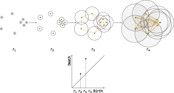
Figure 2: Demonstration of the procedure of topological data analysis. The example persistence diagram here only records the 1-homology classes. Starting from discrete data points as vertices, circles of radius of $r$ are drawn. As $r$ increases and the circles intercept, edges were drawn among the vertices. A series of simplicial complexes are built during the growth of $r$ and the corresponding homology module is recorded into a persistence diagram in the form of the births and deaths of homology generators. The two points in the persistence diagram corresponds to the two circles formed at $r_{2}$ and $r_{3}$ respectively.

II.1 Topology of the principal line bundle: Berry phase

The topological space upon which the Berry phase was defined is the principal line bundle G: ($E,B,\pi,F$), which is associated with the Bloch matrix (4). $B$ is the base manifold as $k\in[-\pi,\pi]$, $F$ is the fiber as the $n$th eigenvector, $E$ is the total space and $\pi$ is the projection map. The Berry phase essentially corresponds to the holonomy class defined on the Hermitian principal line bundle [31, 13]. The expression for the Berry phase is

$$\gamma =\int_{c}i\bra{\Psi_{n}(k)}\frac{\partial}{\partial k}\ket{\Psi_{n}(k)}\,,$$ (5)

where $k$ is the wavenumber, and $\Psi_{n}$ is the $n$th eigenvector of the Bloch matrix. In this paper, we take $n$ to be 1 and will omit the subscript in the following. The expression inside the integral is the connection defined on the Hermitian line bundle with the assumption of adiabatic evolution of the system.

In the physical context, the Berry phase is an extra phase the state picks up while travelling in the parameter space (in this case, the $k$ space) in a closed loop, in addition to the dynamic phase factor which comes from the time-dependent Schrödinger equation (TDSE) [13]. The Berry phase cannot be gauged away, and therefore is physically significant. Below we give a brief derivation of the expression for the Berry phase from this perspective.

We start with

$$\ket{\Psi(t)}\rightarrow e^{i\theta(t)}e^{i\gamma(t)} \ket{\Psi(t)},\qquad\theta(t)=-\frac{1}{\hbar}\int_{0}^{t}E(t^{\prime})dt^{\prime}\,,$$ (6)

where $\ket{\Psi(t)}$ is the state at time $t$, $\theta(t)$ is the dynamic phase factor, and $\gamma(t)$ is the Berry phase.

We then substitute the expression into the TDSE:

$$i\hbar\partial t[e^{i\theta(t)}e^{i\gamma(t)}\ket{\Psi(t)}] =E[e^{i\theta(t)}e^{i\gamma(t)}\ket{\Psi(t)}]\,,$$ (7)

$$\frac{d\gamma}{dt} =i\bra{\Psi(t)}\frac{\partial}{\partial t}\ket{\Psi(t)}\,.$$ (8)

The last step is the variable substitution to arrive at the expression for the Berry phase:

$$\frac{\partial}{\partial t}\ket{\Psi(t)} =\frac{\partial\ket{\Psi(t)}}{\partial k}\frac{\partial k}{\partial t}\,,$$ (9)

$$\gamma =\int_{c}i\bra{\Psi(k^{\prime})}\frac{\partial}{\partial k}\ket{\Psi(k^{\prime})}\,.$$ (10)

The Berry phase as a topological invariant has been shown to be successful in most chiral Hermitian systems. It does not, however, work for all chiral Hermitian systems. For example, recent work has shown that a generalised Berry phase is required for the SSH₄ chain [8].

II.2 Topology of the eigenspace: topological data analysis approach

The topological space topological data analysis (TDA) explores is the projective Hilbert space while the $n$th ($n=1$) state travels in the $k$ space. The projective Hilbert space is the space for $\ket{\psi_{k_{i}}}\bra{\psi_{k_{i}}}$. The metric defined on the projective Hilbert space is fidelity, also known as the Hilbert-Schmidt distance, which describes the geodesic of the states lying on the Bloch sphere, defined as

$$d(\psi_{k_{i}},\psi_{k_{j}})=\sqrt{1-|\bra{\psi_{k_{i}}}\ket{\psi_{k_{j}}}|^{2}}\,.$$ (11)

This approach was introduced in Ref. [18]. We have developed our own in-house program to produce the results reported in this article, and plan to make the program open-sourced.

The topological invariant coming from this projective Hilbert space is its homology class. The idea of this second approach is to use TDA to analyse the homology classes of this space numerically. The next section provides a brief introduction to TDA.

II.2.1 Topological data analysis

Most briefly stated, TDA is a technique that studies a data set using topology (for full details see Ref. [32]). TDA takes a data set as input and calculates the persistence modules of the data set. The basic procedure for calculating $n$th homology modules is as follows: starting from each discrete point, which is considered a vertex in a simplicial complex, an $n$-dimensional ball of radius $r$ is defined centering the vertex. As the $n$-dimensional balls start to intercept with one another, an edge is drawn between the vertices. As $r$ grows larger, a series of simplicial complexes are hence defined. We record the set of simplicial complexes at the point of change in terms of homology as $\{X_{0},X_{1},\ldots,X_{n}\}$, with $X_{0}$ being the trivial homology with $r$ tending to infinity. The corresponding homology module is as follows:

$$H_{p}\mathscr{F}:0=H_{p}(X_{0})\rightarrow H_{p}(X_{1})\rightarrow...$$

$$\rightarrow H_{p}(X_{n})=H_{p}(X)\,,$$ (12)

where $\mathscr{F}$ is the space filtration, and the right arrows represent the inclusion homomorphisms.

The persistence modules can be recorded in persistence diagrams. The persistence diagrams record the births and deaths of $n$-homology classes as $r$ grows larger. An example of how a persistence diagram can represent the homology module is shown in Fig. 2.

A distance metric can be defined in the persistence diagrams space, which is helpful for identifying clusters that correspond to different topological phases. The distance metric between persistence diagrams used here is the Wassterstein distance defined by [32]

$$d(Dgm(\mathscr{F}_{f}), Dgm(\mathscr{F}_{g}))=$$

$$\inf\limits_{x\in\pi}\left[\sum_{x\in Dgm(\mathscr{F}_{f})}(|x-\pi(x)|_{q})^{q}\right]^{1/q}\,,$$ (13)

where $\pi$ is the bijection between two persistence diagrams where all points in the persistence diagrams are considered to be points in $R^{2}$.

II.3 Implementation for the TDA approach

The overall implementation of the TDA approach can be summarised in a series of steps:

Step 1: define the input parameter space for the Bloch matrix.
Step 2: Calculate the persistence diagram for each set of parameters.
Step 3: Conduct cluster analysis on the graph of persistence diagrams.
Step 4: Output the topological phase diagram.

A persistence diagram (step 2) is also calculated in a series of steps:

Step PD1: For each set of parameters, find the optimised list of $k$ samples from $k$ space.
Step PD2: Calculate all eigenvectors corresponding to the list of $k$.
Step PD3: Compute the distance matrix using the fidelity as the distance metric between eigenvectors.
Step PD4: Compute the persistence diagram.

In the above, Step 1 and PD2 are quite self-explanatory. More details associated with the other steps are given as follows.

II.3.1 Step PD1: Optimisation of the sampling of $k$-space

An optimisation procedure is implemented to find a list of $k$ values from $[-\pi,\pi]$ such that the eigenvectors spread in a uniform manner in the eigenspace. This step can ensure the uniform coverage and reduce the noise for the clustering analysis in Step 3.

Step PD1 optimises the sampling of $k$-space by minimising a loss function (details of the numerical implementation are given Appendix A). Here we define our loss function, which is effective and relatively simpler compared to the loss function used in Ref. [18]. If we have the pairwise distances between eigenvectors as the set $L_{d}=\{d(\psi_{k_{0}},\psi_{k_{1}}),d(\psi_{k_{1}},\psi_{k_{2}}),\ldots,d(\psi_{k_{n-1}},\psi_{k_{n}})\}$, where $n$ is the number of samples taken from $k$-space, the loss function is defined as

$$d_{\text{loss}}=\text{std}(L_{d})/\text{mean}(L_{d})\,,$$ (14)

where std and mean refer to the standard deviation and the mean of $L_{d}$.

An example of the effect of the optimisation is shown later in Fig. 5(a)-(d). The implications of the result will be discussed in the results section.

II.3.2 Steps PD3-PD4: generating all the persistence diagrams for all sets of parameters in the parameter space

The inputs required to generate the persistence diagrams are pair-wise distances between the eigenvectors stored in distance matrices (where $D_{ij}=d(\psi_{k_{i}},\psi_{k_{j}})$) (for details of the numerical implementation see Appendix A). After repeating for all sets of parameters for steps PD3 and PD4, all distance matrices for the eigenspaces and the corresponding persistence diagrams are calculated.

II.3.3 Step 3: clustering analysis of persistence diagrams

Once all the persistence diagrams for all sets of parameters are collected, we define a weighted graph G = ($V,E,w$) for the persistence diagrams, where $V$ and $E$ are the sets of vertices and edges respectively, and $w$ is a mapping from the edges to their corresponding weights: $w:E\rightarrow R$. The vertices $V$ are the persistence diagrams corresponding to different parameter sets, and the edge weights are defined with the distance between the persistence diagrams:

$$w_{ij}=\exp{-W_{2}(PD_{i},PD_{j})/\overline{W_{2}}}\,,$$ (15)

where $W_{2}$ refers to the Wasserstein distance (II.2.1) between persistence diagrams with $q$ set to 2. Only the 1-homology was included in the persistence diagrams. $\overline{W_{2}}$ refers to the average Wassterstein distance among all persistence diagrams.

Since the different topology within each region in the parameter space will be captured by the persistence diagrams, clustering analysis of the graph of persistence diagrams will give us the topological phase diagram directly. For the clustering analysis, an unsupervised spectral clustering method is used [33]. In the same way as Ref. [18], we define a random walk Laplacian as

$$L=1-D^{-1}W\,,$$ (16)

where $W$ is the adjacency matrix where $W_{i,j}=w_{ij}$ and $D$ is a diagonal matrix, where $D_{ij}=\sum_{j}w_{ij}$.

The clustering analysis starts by taking lowest eigenvalues and plotting the corresponding eigenvectors. The lowest eigenvalues of the Laplacian signal the existence of clusters in the graph, and the space where clustering analysis takes place involves the eigenvectors corresponding to those eigenvalues. Following Ref. [18], $k$-means clustering was used to detect the clusters on the embedding of the eigenvectors to $R^{n}$.

II.4 The relationship between the two approaches

It is worth noting that the Berry phase and fidelity are connected through the geometric quantum tensor. As shown in Refs. [34, 35], the imaginary part of the geometric tensor can be related to the Berry curvature, while the real part of the geometric tensor is the fidelity, which is the geodesic of the states lying on the Bloch sphere.

III Results

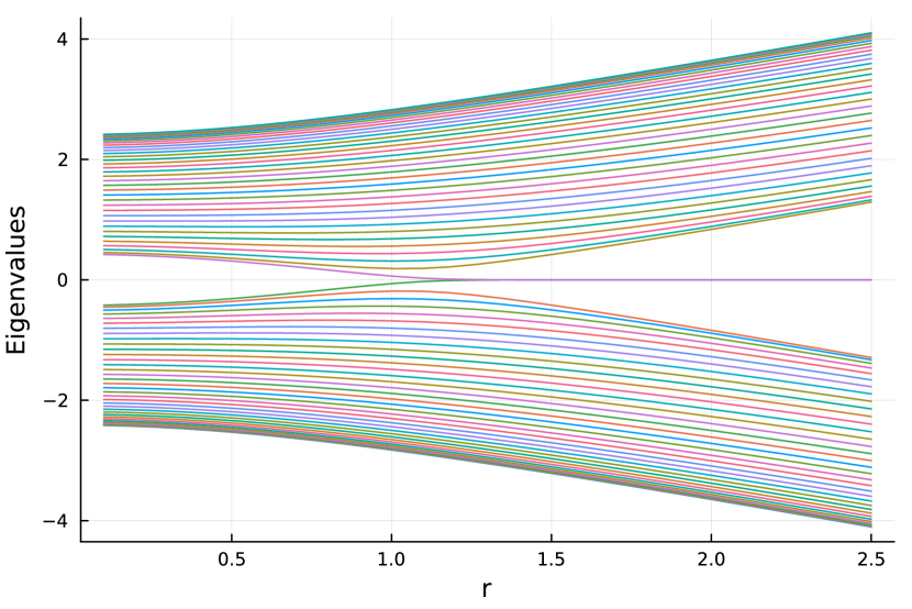
(a)

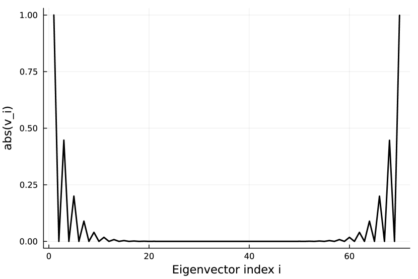
(b)

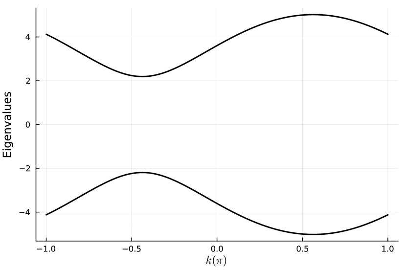
(c)

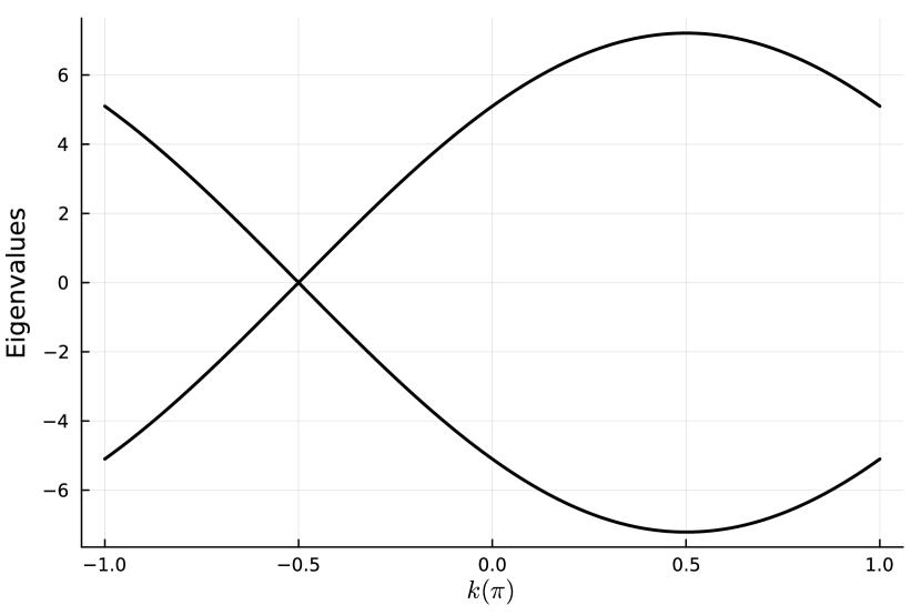
(d)

(e)

Figure 3: (a) The eigenspectrum of the complex SSH model with $v=1+i$ and $w=1+r\,i$, for $N=70$. The phase transition occurs at $r=1$. When $r>1$, $|v|<|w|$, and a zero energy state can be observed. (b) When $|v|<|w|$, zero energy eigenvectors can be observed in the form of an edge state. (c)-(e) The eigenspectrum for the Bloch Hamiltonian for ($v$,$w$) values (2 + 3 i, 1 + i), (1 + i, 2 + 3 i), (2 + 3i, 3 + 2i), respectively.

In this section we explore the topological features of the complex SSH model. The complex extension of this model, unsurprisingly, possesses all the topological behaviour observed in the original SSH model as well as the bulk-boundary correspondence. We have found that there are two topological phases for the complex SSH model, being $|v|<|w|$ and $|v|>|w|$. If $v$ and $w$ are real, as in the case of the original SSH model, the two topological phases reduce to $v<w$ and $v>w$.

Analysis of both the topology of the principal line bundle and the eigenspace are shown here. This includes numerical results for the Berry phase and the results of the TDA approach.

III.1 Eigenspectrum and the bulk-boundary correspondence of the complex SSH

As can be seen in Fig. 3, the overall spectrum behaviour is similar to that of the real SSH model. The number of sites is chosen as even in Fig. 3 without loss of generality. Two zero-energy states can be observed when $|v|<|w|$, corresponding to the edge states, which are shown in Fig. 3(b).

The topological phase transition points, where edge states start to occur, can also be predicted through the Bloch Hamiltonians alone. This shows clear signs of the existence of bulk-boundary correspondence. As shown in Fig. 3(c)-(e), the band gap closes at $|v|=|w|$, which is where the zero energy edge states begin to appear in the open system.

III.2 Numerical results for the Berry phase

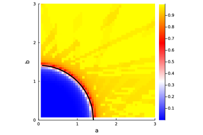
Figure 4: Numerical result for the Berry phase with $v=1+i$ and $w=a+b\,i$. The yellow and blue regions correspond to topological and trivial respectively. The black line is a line plot for a perfect circle with radius $\sqrt{2}$ as a guide for the eye.

The analytical solution for equation (4) is simply

$$\ket{\pm k}=\begin{bmatrix}\pm e^{-i\phi(k)}\\ 1\end{bmatrix}\,,$$ (17)

where

$$\tan(\phi(k))=\frac{(v_{R}w_{R}+v_{i}w_{i}+|w|^{2}\cos k)\sin k}{|v|^{2}+2(v_{R}w_{R}+v_{i}w_{i})\cos k+|w|^{2}\cos 2k}\,.$$ (18)

Thus the Berry phase can be calculated as

$$\gamma =\frac{1}{2\pi}\int_{c}\frac{d\phi}{dk}dk\,.$$ (19)

The numerical calculation of the Berry phase is shown in Fig. 4. Numerical noise aside, it can be observed clearly that there are two topological phases, being inside and outside the circle. It supports our conclusion that $|v|=|w|$ is the phase transition point. When $|v|>|w|$, the complex SSH model is topological trivial with Berry phase value 0. On the other hand, when $|v|<|w|$, the complex SSH model possesses and edge state and is therefore topological non-trivial, with a non-zero Berry phase, 1.

III.3 Topological data analysis of the projected Hilbert space

(a)

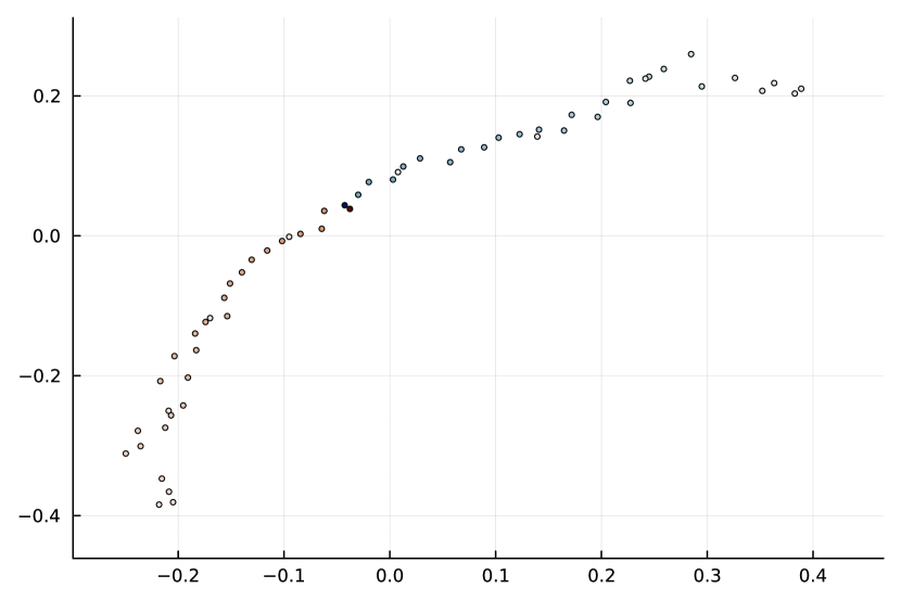
(b)

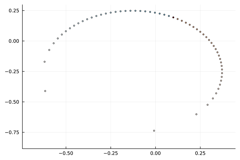
(c)

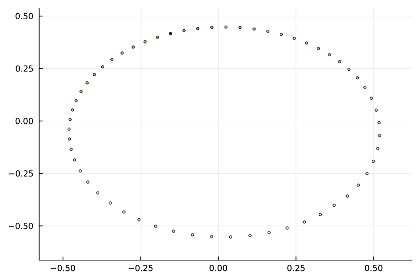
(d)

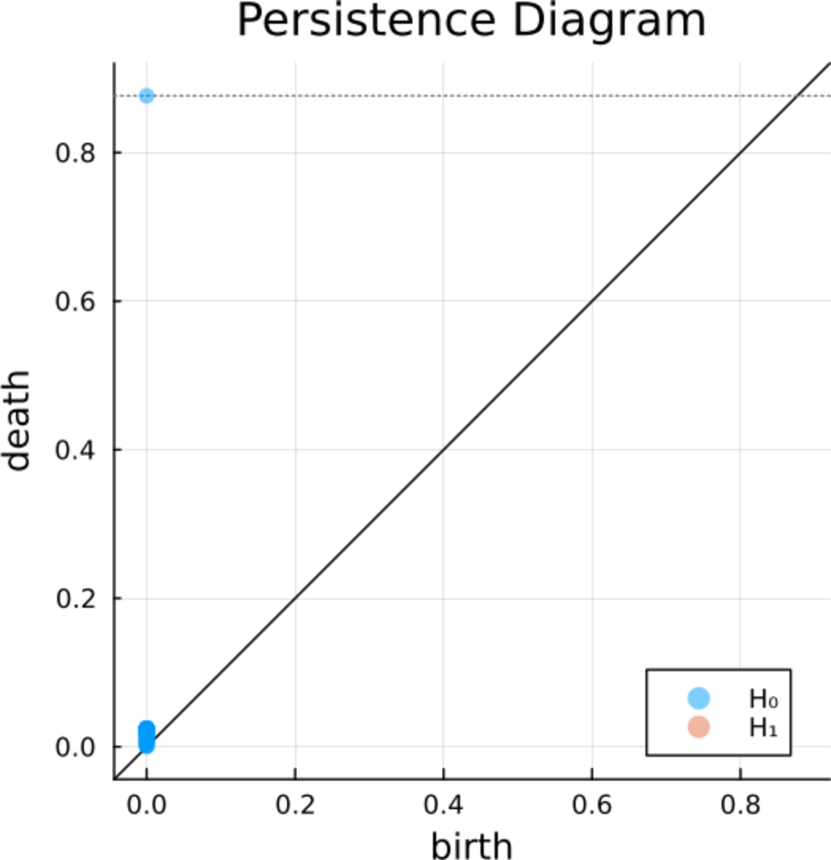
(e)

(f)

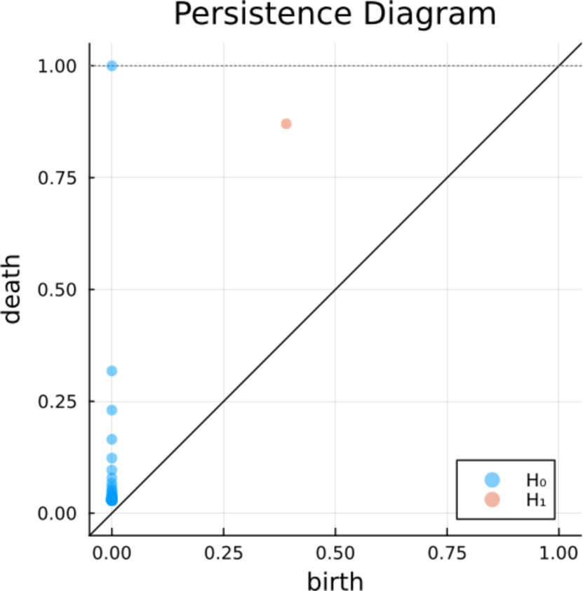
(g)

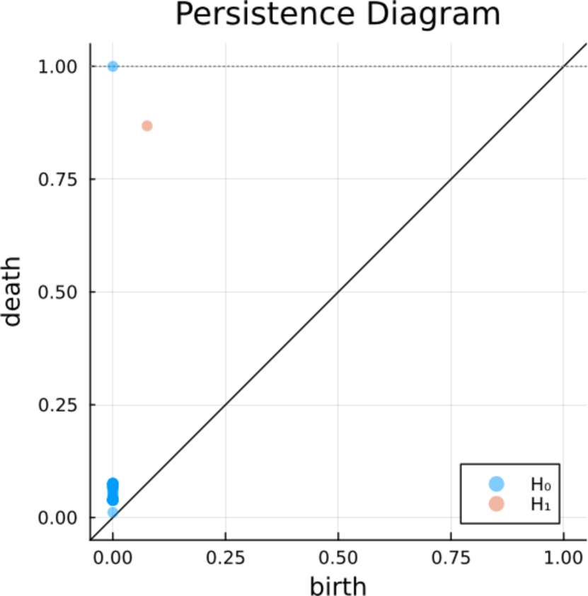
(h)

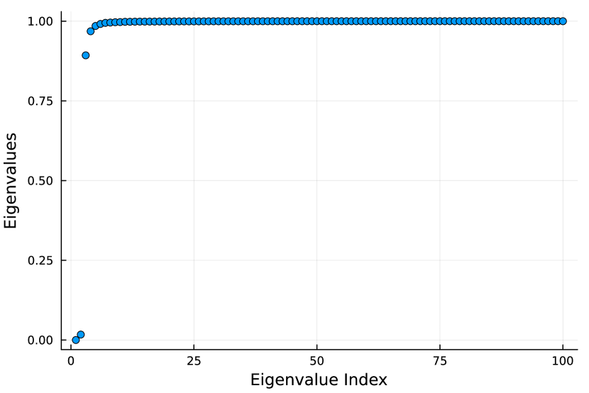
(i)

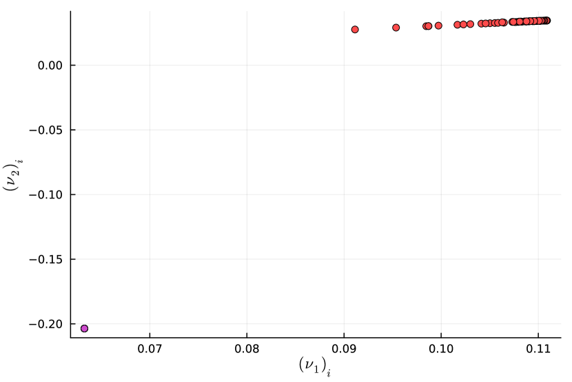
(j)

Figure 5: (a) & (c) The multi-dimensional scaling (MDS) projection of the eigenspaces into the Euclidean space without optimisation (Step PD1 in Section II.3) for $v=0.8+1.4i$, $w=1+1i$, and $v=1+1i$, $w=0.8+1.4i$, respectively. (b) & (d) The corresponding MDS projection of the eigenspace into the Euclidean space with optimisation for $v=0.8+1.4i$, $w=1+1i$, and $v=1+1i$, $w=0.8+1.4i$, respectively. (e)-(h) The corresponding persistence diagrams of the eigenspaces above. (i) The eigenvalues for the random walk Laplacian for the graph of persistence diagrams, with edge weights defined by equation (15). Two values lower than 0.2 were considered to represent two clusters (j) The first two smallest eigenvectors plotted against each other for $k$-means cluster analysis. The purple cluster at the bottom left correspond to the persistence diagrams where $|v|>|w|$ , and the red cluster correspond to the persistence diagrams where $|v|<|w|$.

Similar to the analysis given in Ref. [18], we show that the topology of the eigenspace is sufficient to arrive at the same topological phase diagram for the complex SSH model generated using the Berry phase.

In Fig. 5, we show first how the topology of the eigenspace is different going from the topologically trivial region to the topologically non-trivial region, and how optimisation can make that difference clearer (Fig. 5(a)-(h)). We then show the result of the clustering analysis and the conclusion for the topological phase diagram, which agrees with the results of Section III.2 (Fig. 5(i)-(j)).

We start by showing the difference in topology going from one phase to another. Two sets of parameters were chosen from regions $|v|>|w|$ and $|v|<|w|$. As shown in Fig. 5(a) and (c), we see that if $|v|>|w|$, no circles can be observed from the eigenspace, while a circle is shown when $|v|<|w|$. It is important to note here that both Fig. 5(a) and (c) are projections from the projective Hilbert space to Euclidean space through Multidimensional scaling (MDS) [36]. They are faithful representations in terms of the pair-wise distances between the data points. However, they are for visualization purposes only and the persistence diagram calculations rely on the distance matrices defined in Section II.3.

Fig. 5 also shows that the optimisation step (from Section. II.3) reduces the potential noise present in the system. From Fig. 5(a) to 5(b), and 5(c) to 5(d), we can see that the spread of the samples from the eigenspace is more uniform and the existence or non-existence of a circle is more obvious after optimisation.

Such improvement from optimisation is reflected clearly in the corresponding persistence diagrams. Overall, the persistence diagrams in Fig. 5(e) and (f) show no 1-homology generators, while Fig. 5(g) and (h) show the existence of one homology generator. The effect of the optimisation step is made clear from the comparison between Fig. 5(g) and (f). While both persistence diagrams show the existence of one 1-homology generator, the 1-homology generator shown after optimisation has a longer life expectancy. This extended life of the 1-homology generator after optimisation is reflected by the relative position of the corresponding data point to the diagonal line.

Fig. 5(i) and (j) shows the result of the $k$-means clustering analysis of the persistence diagrams (Step 3 in Section II.3). Fig. 5(i) shows the eigenvalues of the random walk Laplacian. We observed that there are two eigenvalues that are very close to zero, which signal two clusters in the graph. If we plot the first two eigenvectors against each other (shown in Fig. 5(j)), $k$-means can identify those two clusters. It can be shown that the two clusters correspond to the two topological phases identified by Berry phase. The purple cluster at the bottom left corresponds to the region where $|v|>|w|$ and the Berry phase is zero; the red cluster at the top right corresponds to the region where $|v|<|w|$ and the Berry phase is 1.

Therefore, it is clear that the two clusters shown in Fig. 5(j) correspond to the two regions in the topological phase diagram generated using the Berry phase (see Fig. 4).

IV Conclusion

We have used two methods – Berry phase and topological data analysis – to explore the topological properties of the complex SSH model. Our findings demonstrate that both methods can generate topological phase diagrams for the model, identifying two distinct regions based on the relative magnitudes of the complex parameters $|v|$ and $|w|$. Specifically, we find that when $|v|>|w|$, the system is topologically trivial, whereas for $|v|<|w|$, it exhibits topologically non-trivial behavior. These results provide insights into the topological properties of the complex SSH model and highlight the complementary potential of the two methods in the topological analysis of the SSH-type models. We have specifically focused on the Hermitian version of the complex SSH model as a first step towards testing and exploring the limitations and potential generalisations of topological approaches on the more complicated SSH models, including their non-Hermitian extensions.

Appendix A Numerical details for step 2

In the step PD1, Flux is the Julia package used to implement the optimisation of the sampling of $k$-space. Adam, which is an extension to the stochastic gradient descent algorithm, was chosen in Flux to optimise the sampling [37, 38].

The package we used to calculate the persistence diagrams is a pure Julia implementation of the Ripser algorithm, Ripserer [39, 40].

Appendix B Analytical solution for the complex SSH model

The tridiagonal matrix of size $N\times N$ in the basis $\ket{m,A/B}$ for the complex SSH Hamiltonian (1) is of the form

$H$ = $\begin{bmatrix}0&v&0&0&0&0&\dots\\ v^{*}&0&w&0&0&0&\dots\\ 0&w^{*}&0&v&0&0&\dots\\ 0&0&v^{*}&0&w&0&\dots\\ 0&0&0&w^{*}&0&v&\dots\\ 0&0&0&0&v^{*}&0&\dots\\ \vdots&\ldots&\\ 0&&&&&&\ldots&0\end{bmatrix}$  .

B.1 The case when $N$ is odd, $\lambda\not=0$

As noted in the solution of the SSH model with real $v$ and $w$ [41], the diagonalisation of such a matrix has been discussed in the mathematics literature [42], from which we can make use of Lemma 1 [42] in terms of the definition

$$T(\alpha,\beta,n)=\alpha^{n}+\alpha^{n-1}\beta+\cdots+\alpha\beta^{n-1}+\beta^{n}\,.$$ (20)

Lemma 1. Let $\alpha$ and $\beta$ be nonzero complex numbers. Then the Fibonacci-type sequence $\{a_{n}\}^{\infty}_{n=1}$ defined as

$$a_{n+2}-(\alpha+\beta)a_{n+1}+\alpha\beta a_{n}=0,~{}~{}n=1,2,\ldots$$ (21)

can be represented in terms of $a_{1}$ and $a_{2}$ by

$$a_{n}=T(\alpha,\beta,n-2)a_{2}-\alpha\beta T(\alpha,\beta,n-3)a_{1},~{}~{}n=1,2,\ldots$$ (22)

Following [42], if $N=2M+1$, the eigenvector components satisfy the set of equations

$$vx_{2} =\lambda x_{1},$$ (23)

$$w^{*}x_{2M} =\lambda x_{2M+1},$$ (24)

$$v^{*}x_{2n-1}+wx_{2n+1} =\lambda x_{2n},$$ (25)

$$w^{*}x_{2n}+vx_{2n+2} =\lambda x_{2n+1},$$ (26)

where $\lambda$ are the eigenenergies.

From equations (25) and (26), we have

$$x_{2n+3}+\frac{vv^{*}+ww^{*}-\lambda^{2}}{vw}x_{2n+1}+\frac{w^{*}v^{*}}{wv}x_{2n-1} =0.$$ (27)

$$x_{2n+2}+\frac{vv^{*}+ww^{*}-\lambda^{2}}{vw}x_{2n}+\frac{w^{*}v^{*}}{wv}x_{2n-2} =0.$$ (28)

Therefore, we can choose $\alpha$ and $\beta$ such that

$$\alpha+\beta =\frac{vv^{*}+ww^{*}-\lambda^{2}}{vw}x_{2n+1},$$ (29)

$$\alpha\beta =\frac{w^{*}v^{*}}{wv}.$$ (30)

From equations (23)-(26), we have

$$x_{2} =\frac{\lambda}{v}x_{1},$$ (31)

$$x_{3} =\left[\frac{v(\alpha+\beta)+w^{*}}{v}\right]x_{1},$$ (32)

$$x_{4} =\frac{\lambda(\alpha+\beta)}{v}x_{1}.$$ (33)

Combining Lemma 1 with these equations then gives

$$x_{2n-1} =\left[\frac{w^{*}}{v}T(\alpha,\beta,n-2)+T(\alpha,\beta,n-1)\right]x_{1},$$ (34)

$$x_{2n} =\frac{\lambda}{v}T(\alpha,\beta,n-1)x_{1}.$$ (35)

Now combining this result with equation (24) gives

$$T(\alpha,\beta,N)=0\,.$$ (36)

Therefore we have

$$\alpha^{M+1}-\beta^{M+1} =0\,,$$ (37)

$$|\alpha| =|\beta|\,.$$ (38)

A natural choice for $\alpha$ and $\beta$ follows as

$$\alpha=\frac{w^{*}}{w}\exp{ki}\,,\quad\beta=\frac{v^{*}}{v}\exp{-ki}\,.$$ (39)

Substitution into (37) then gives

$$\left(\frac{w^{*}}{w}\right)^{M+1} \exp{ik(M+1)}$$

$$-\left(\frac{v^{*}}{v}\right)^{M+1} \exp{-ik(M+1)}=0\,.$$ (40)

When $\frac{w^{*}}{w}=\frac{v^{*}}{v}$, the solution reduces to

$$k=\frac{n\pi}{M+1},\quad n\in[1,M]\,.$$ (41)

In summary, we have the eigenvalues in the form

$$\lambda=\pm\sqrt{|v|^{2}+|w|^{2}+vw(\alpha+\beta)}\,,$$ (42)

where $\alpha$ and $\beta$ are defined in (39) and $k$ needs to be solved from equation (B.1). The eigenvector components are given by equations (34) and (35).

B.2 The case when $N$ is even, $\lambda\not=0$

Again following Ref. [42], if $N=2M$, we have the set of equations

$$vx_{2} =\lambda x_{1}\,,$$ (43)

$$v^{*}x_{2M-1} =\lambda x_{2M}\,,$$ (44)

$$v^{*}x_{2n-1}+wx_{2n+1} =\lambda x_{2n}\,,$$ (45)

$$w^{*}x_{2n}+vx_{2n+2} =\lambda x_{2n+1}\,.$$ (46)

Combining these equations with (34) and (35) gives

$$\frac{v^{*}w^{*}}{v}T(\alpha,\beta,M-2)+v^{*}T(\alpha,\beta,M-1)$$

$$=\frac{\lambda^{2}}{v}T(\alpha,\beta,M-1)\,.$$ (47)

The eigenvalue expression is the same as equation (42). The eigenvectors are as given in (34) and (35), where $k$ needs to be solved using the anstaz in (39) in combination with (B.2), which can be readily done.

B.3 $\lambda=0$

From equations (23), (25) and (26), the form of the eigenvectors for the zero energy edge states is

$$x_{2n+1} =\left(-\frac{v^{*}}{w}\right)^{n}x_{2n-1}\,,$$ (48)

$$x_{2n} =0\,.$$ (49)

References

- Su et al. [1979] W. Su, J. Schrieffer, and A. J. Heeger, Solitons in polyacetylene, Physical Review Letters 42, 1698 (1979).
- Pérez-González et al. [2018] B. Pérez-González, M. Bello, Á. Gómez-León, and G. Platero, SSH model with long-range hoppings: topology, driving and disorder, arXiv preprint arXiv:1802.03973 (2018).
- Kitaev [2003] A. Y. Kitaev, Fault-tolerant quantum computation by anyons, Annals of physics 303, 2 (2003).
- Plugge et al. [2017] S. Plugge, A. Rasmussen, R. Egger, and K. Flensberg, Majorana box qubits, New Journal of Physics 19, 012001 (2017).
- Li et al. [2015] L. Li, C. Yang, and S. Chen, Winding numbers of phase transition points for one-dimensional topological systems, Europhysics Letters 112, 10004 (2015).
- Li and Miroshnichenko [2018] C. Li and A. E. Miroshnichenko, Extended SSH model: Non-local couplings and non-monotonous edge states, Physics 1, 2 (2018).
- Li et al. [2014] L. Li, Z. Xu, and S. Chen, Topological phases of generalized Su-Schrieffer-Heeger models, Physical Review B 89, 085111 (2014).
- Anastasiadis et al. [2022] A. Anastasiadis, G. Styliaris, R. Chaunsali, G. Theocharis, and F. K. Diakonos, Bulk-edge correspondence in the trimer Su-Schrieffer-Heeger model, Physical Review B 106, 085109 (2022).
- Alvarez and Coutinho-Filho [2019] V. M. Alvarez and M. Coutinho-Filho, Edge states in trimer lattices, Physical Review A 99, 013833 (2019).
- Otaki and Fukui [2019] Y. Otaki and T. Fukui, Higher-order topological insulators in a magnetic field, Physical Review B 100, 245108 (2019).
- Liu et al. [2022] Q. Liu, K. Wang, J.-X. Dai, and Y. Zhao, Takagi topological insulator on the honeycomb lattice, Frontiers in Physics , 400 (2022).
- Berry [1984] M. V. Berry, Quantal phase factors accompanying adiabatic changes, Proceedings of the Royal Society of London. A. Mathematical and Physical Sciences 392, 45 (1984).
- Böhm et al. [2003] A. Böhm, A. Mostafazadeh, H. Koizumi, Q. Niu, and J. Zwanziger, The Geometric phase in quantum systems: foundations, mathematical concepts, and applications in molecular and condensed matter physics (Springer, 2003).
- Chen [2021] Z. Chen, A mathematical formalism of non-Hermitian quantum mechanics and observable-geometric phases, arXiv preprint arXiv:2111.12883 (2021).
- Yao and Wang [2018] S. Yao and Z. Wang, Edge states and topological invariants of non-Hermitian systems, Physical Review Letters 121, 086803 (2018).
- Kawabata et al. [2019] K. Kawabata, K. Shiozaki, M. Ueda, and M. Sato, Symmetry and topology in non-Hermitian physics, Physical Review X 9, 041015 (2019).
- Tsubota et al. [2022] S. Tsubota, H. Yang, Y. Akagi, and H. Katsura, Symmetry-protected quantization of complex Berry phases in non-Hermitian many-body systems, Physical Review B 105, L201113 (2022).
- Park et al. [2022] S. Park, Y. Hwang, and B.-J. Yang, Unsupervised learning of topological phase diagram using topological data analysis, Physical Review B 105, 195115 (2022).
- Gong et al. [2018] Z. Gong, Y. Ashida, K. Kawabata, K. Takasan, S. Higashikawa, and M. Ueda, Topological phases of non-Hermitian systems, Physical Review X 8, 031079 (2018).
- Yu and Deng [2021] L.-W. Yu and D.-L. Deng, Unsupervised learning of non-hermitian topological phases, Physical Review Letters 126, 240402 (2021).
- Zhou and Lee [2019] H. Zhou and J. Y. Lee, Periodic table for topological bands with non-Hermitian symmetries, Physical Review B 99, 235112 (2019).
- Cheng and Yu [2021] Z. Cheng and Z. Yu, Supervised machine learning topological states of one-dimensional non-Hermitian systems, Chinese Physics Letters 38, 070302 (2021).
- Ryu et al. [2012] J.-W. Ryu, S.-Y. Lee, and S. W. Kim, Analysis of multiple exceptional points related to three interacting eigenmodes in a non-Hermitian Hamiltonian, Physical Review A 85, 042101 (2012).
- Asbóth et al. [2016] J. K. Asbóth, L. Oroszlány, and A. Pályi, A short course on topological insulators, Lecture Notes in Physics 919, 166 (2016).
- Batra and Sheet [2019] N. Batra and G. Sheet, Understanding basic concepts of topological insulators through Su-Schrieffer-Heeger (SSH) model, arXiv preprint arXiv:1906.08435 (2019).
- Sedlmayr et al. [2018] N. Sedlmayr, P. Jaeger, M. Maiti, and J. Sirker, Bulk-boundary correspondence for dynamical phase transitions in one-dimensional topological insulators and superconductors, Physical Review B 97, 064304 (2018).
- Koch and Budich [2020] R. Koch and J. C. Budich, Bulk-boundary correspondence in non-Hermitian systems: stability analysis for generalized boundary conditions, The European Physical Journal D 74, 1 (2020).
- Prodan and Schulz-Baldes [2016] E. Prodan and H. Schulz-Baldes, Bulk and boundary invariants for complex topological insulators: From K-Theory to Physics (Springer, 2016).
- Yokomizo and Murakami [2019] K. Yokomizo and S. Murakami, Non-Bloch band theory of non-Hermitian systems, Physical Review Letters 123, 066404 (2019).
- Xiong [2018] Y. Xiong, Why does bulk boundary correspondence fail in some non-Hermitian topological models, Journal of Physics Communications 2, 035043 (2018).
- Simon [1983] B. Simon, Holonomy, the quantum adiabatic theorem, and Berry’s phase, Physical Review Letters 51, 2167 (1983).
- Dey and Wang [2022] T. K. Dey and Y. Wang, Computational topology for data analysis (Cambridge University Press, 2022).
- Von Luxburg [2007] U. Von Luxburg, A tutorial on spectral clustering, Statistics and computing 17, 395 (2007).
- Cheng [2010] R. Cheng, Quantum geometric tensor (fubini-study metric) in simple quantum system: A pedagogical introduction, arXiv preprint arXiv:1012.1337 (2010).
- Carollo et al. [2020] A. Carollo, D. Valenti, and B. Spagnolo, Geometry of quantum phase transitions, Physics Reports 838, 1 (2020).
- Pedregosa et al. [2011] F. Pedregosa, G. Varoquaux, A. Gramfort, V. Michel, B. Thirion, O. Grisel, M. Blondel, P. Prettenhofer, R. Weiss, V. Dubourg, J. Vanderplas, A. Passos, D. Cournapeau, M. Brucher, M. Perrot, and E. Duchesnay, Scikit-learn: Machine learning in Python, Journal of Machine Learning Research 12, 2825 (2011).
- Innes et al. [2018] M. Innes, E. Saba, K. Fischer, D. Gandhi, M. C. Rudilosso, N. M. Joy, T. Karmali, A. Pal, and V. Shah, Fashionable modelling with flux, CoRR abs/1811.01457 (2018), arXiv:1811.01457 .
- Innes [2018] M. Innes, Flux: Elegant machine learning with julia, Journal of Open Source Software 10.21105/joss.00602 (2018).
- Čufar [2020] M. Čufar, Ripserer.jl: flexible and efficient persistent homology computation in julia, Journal of Open Source Software 5, 2614 (2020).
- Čufar and Žiga Virk [2021] M. Čufar and Žiga Virk, Fast computation of persistent homology representatives with involuted persistent homology (2021), arXiv:2105.03629 [math.AT] .
- Sirker et al. [2014] J. Sirker, M. Maiti, N. Konstantinidis, and N. Sedlmayr, Boundary fidelity and entanglement in the symmetry protected topological phase of the SSH model, Journal of Statistical Mechanics: Theory and Experiment 2014, P10032 (2014).
- Shin [1997] B. C. Shin, A formula for eigenpairs of certain symmetric tridiagonal matrices, Bulletin of the Australian Mathematical Society 55, 249 (1997).