Probing Ultra-late Reionization: Direct Measurements of the Mean Free Path over $5<z<6$

Abstract

The mean free path of ionizing photons, $\lambda_{\rm mfp}$, is a critical parameter for modeling the intergalactic medium (IGM) both during and after reionization. We present direct measurements of $\lambda_{\rm mfp}$ from QSO spectra over the redshift range $5<z<6$, including the first measurements at $z\simeq 5.3$ and 5.6. Our sample includes data from the XQR-30 VLT large program, as well as new Keck/ESI observations of QSOs near $z\sim 5.5$, for which we also acquire new [C II] 158$\mu$m redshifts with ALMA. By measuring the Lyman continuum transmission profile in stacked QSO spectra, we find $\lambda_{\rm mfp}=9.33_{-1.80}^{+2.06}$, $5.40_{-1.40}^{+1.47}$, $3.31_{-1.34}^{+2.74}$, and $0.81_{-0.48}^{+0.73}$ pMpc at $z=5.08$, 5.31, 5.65, and 5.93, respectively. Our results demonstrate that $\lambda_{\rm mfp}$ increases steadily and rapidly with time over $5<z<6$. Notably, we find that $\lambda_{\rm mfp}$ deviates significantly from predictions based on a fully ionized and relaxed IGM as late as $z=5.3$. By comparing our results to model predictions and indirect $\lambda_{\rm mfp}$ constraints based on IGM Ly$\alpha$ opacity, we find that the $\lambda_{\rm mfp}$ evolution is consistent with scenarios wherein the IGM is still undergoing reionization and/or retains large fluctuations in the ionizing UV background well below redshift six.

1 Introduction

When and how reionization occurred is a fundamental question about the early universe and the first galaxies. The appearance of transmitted flux in the Lyman-$\alpha$ (Ly$\alpha$) forest of high-redshift QSOs (e.g., Fan et al., 2006) has long been interpreted as evidence that hydrogen in the intergalactic medium (IGM) was largely reionized by $z=6$. In terms of the ionizing photon budget, however, an end of reionization at $z\geq 6$ is challenging to reconcile with a midpoint of $z\sim 7-8$ suggested by e.g., cosmic microwave background (CMB) observations (Planck Collaboration et al., 2020, see also de Belsunce et al., 2021). In particular, star-forming galaxies at $z>6$ would have to emit ionizing photons extremely efficiently in order to complete reionization within such a short interval. This leaves two possibilities: the ionizing efficiency of galaxies at $z>6$ is remarkably high, and/or reionization extends to lower redshifts.

A number of observations have now been used to constrain the timeline of reionization. These observations include the Ly$\alpha$ damping wing in $z\gtrsim 7$ QSO spectra (e.g., Bañados et al., 2018; Davies et al., 2018; Wang et al., 2020; Yang et al., 2020a; Greig et al., 2021), the decline in observed Ly$\alpha$ emission from galaxies at $z>6$ (e.g., Mason et al., 2018, 2019; Hoag et al., 2019; Hu et al., 2019, and references therein, but see Jung et al., 2020; Wold et al., 2021), and measurements of the thermal state of the IGM at $z>5$ (e.g., Boera et al., 2019; Gaikwad et al., 2021). These observations support a midpoint of reionization at $z\sim 7-8$ and are generally consistent with an ending point at $z\sim 6$, as constrained by the fraction of dark pixels in the Ly$\alpha$ forest (e.g., McGreer et al., 2015, but see Zhu et al., 2022).

Other observations, however, suggest that reionization may have extended to significantly lower redshifts. Large-scale fluctuations in the measured Ly$\alpha$ effective optical depth (e.g., Fan et al., 2006; Becker et al., 2015; Eilers et al., 2018; Bosman et al., 2018, 2022; Yang et al., 2020b), together with long troughs extending down to or below $z\simeq 5.5$ in the Ly$\alpha$ forest (e.g., Becker et al., 2015; Zhu et al., 2021), potentially indicate the existence of large neutral IGM islands (e.g., Kulkarni et al., 2019; Keating et al., 2020b; Nasir & D’Aloisio, 2020; Qin et al., 2021). This interpretation is further supported by dark gaps in the Ly$\beta$ forest (Zhu et al., 2022). Reionization extending to $z<6$ is also consistent with the observed underdensities around long dark gaps traced by Ly$\alpha$ emitting galaxies (LAEs, Becker et al., 2018; Kashino et al., 2020; Christenson et al., 2021). In addition, such a late-ending reionization scenario is consistent with the evolution of metal-enriched absorbers at $z\sim 6$ (e.g., Becker et al., 2019; Davies et al., 2023a, b), as well as numerical models that reproduce a variety of observations (e.g., Weinberger et al., 2019; Choudhury et al., 2021; Qin et al., 2021; Gaikwad et al., 2023).

A potentially decisive clue for establishing when reionization ended comes from recent measurements of the mean free path of ionizing photons ($\lambda_{\rm mfp}$). Becker et al. (2021, herein referred to as B21) found that the $\lambda_{\rm mfp}$ increases by a factor of around ten between $z=6.0$ and 5.1, and the $\lambda_{\rm mfp}$ at $z=6.0$ is about eight times shorter than what would be expected based on its evolution at $z\lesssim 5$ (see also constraints from Bosman, 2021). Such a rapid evolution in the $\lambda_{\rm mfp}$ is expected to occur near the end of reionization due to (i) the growth and merger of ionized bubbles, and (ii) the photo-evaporation of dense, optically thick sinks (e.g., Shapiro et al., 2004; Furlanetto & Oh, 2005; Sobacchi & Mesinger, 2014; Park et al., 2016; D’Aloisio et al., 2020). Furthermore, the $\lambda_{\rm mfp}$ measurements in B21 are difficult to reconcile with models where reionization completes at $z>6$, and may instead support models where the IGM is still $\gtrsim 20\%$ neutral at $z=6$ (Becker et al., 2021; Cain et al., 2021; Davies et al., 2021).

Our understanding of how $\lambda_{\rm mfp}$ evolves over $5<z<6$ is highly incomplete, however. The measurements of B21 were restricted to $z\simeq 5.1$ and $\simeq 6.0$ by a lack of high-quality spectra at intermediate redshifts. This was due to a historical redshift gap in the discovery of QSOs near $z\sim 5.5$, which have overlap with brown dwarfs in their visible colors. This gap, however, has been filled by Yang et al. (2017, 2019) using near- and mid-infrared photometry, making it possible to obtain a significant sample of high-quality $z\sim 5.5$ QSO spectra for the first time.

In this work, we report the first measurements of $\lambda_{\rm mfp}$ at multiple redshifts between $z=6$ and 5. In addition to archival QSO spectra used in B21, our sample includes new QSO spectra from the XQR-30 VLT large program (e.g., D’Odorico et al., 2023; Bischetti et al., 2022; Bosman et al., 2022; Chen et al., 2022; Davies et al., 2023a; Lai et al., 2022; Satyavolu et al., 2023; Zhu et al., 2021, 2022) as well as from new Keck/ESI observations. This paper is organized as follows. In Section 2, we describe the data and observations. Section 3 briefly introduces the methods we use to measure the $\lambda_{\rm mfp}$. We present our results and discuss their implications for reionization in Section 4. Finally, we summarize our findings in Section 5. Throughout this paper we assume a $\Lambda$CDM cosmology with $\Omega_{\rm m}=0.3$, $\Omega_{\Lambda}=0.7$, and $h=0.7$. Distances are quoted in proper units unless otherwise noted. We also use 912 Å to represent the Lyman limit wavelength of 911.76 Å.

2 Data and Observations

To measure $\lambda_{\rm mfp}$ over $5<z<6$, we employ a large sample of 97 spectra of QSOs at $4.9<z<6.1$. Our sample includes 23 LRIS spectra and 35 GMOS spectra of QSOs at $z\lesssim 5.3$ used in B21. For higher redshifts, we use 18 and 6 spectra from the Keck/ESI (Sheinis et al., 2002) and VLT/X-Shooter (Vernet et al., 2011) archives, respectively. We include 7 high-quality spectra with sufficient wavelength coverage from the XQR-30 VLT large program (D’Odorico et al., 2023). The rest of the data are new spectra of 8 QSOs near $z\sim 5.5$ from our ESI observations. A summary of our QSO sample is provided in Table 2.

Table 1: QSO Spectra Used for $\lambda_{\rm mfp}$ Measurements

QSO	RA (J2000)	DEC (J2000)	$z_{\rm qso}$	Ref	Instrument	$M_{1450}$	Ref	$R_{\rm eq}\,\rm(pMpc)$
J0015$-$0049	00:15:29.86	$-$00:49:04.3	$4.931$	a	LRIS	$-25.2$	$\alpha$	$3.8^{+1.1}_{-0.8}$
J0256$+$0002	02:56:45.75	$+$00:02:00.2	$4.960$	a	LRIS	$-24.6$	$\alpha$	$2.8^{+0.9}_{-0.6}$
J0236$-$0108	02:36:33.83	$-$01:08:39.2	$4.974$	a	LRIS	$-25.0$	$\alpha$	$3.4^{+1.1}_{-0.7}$
J0338$+$0018	03:38:30.02	$+$00:18:40.0	$4.988$	a	LRIS	$-25.1$	$\alpha$	$3.5^{+1.2}_{-0.7}$
J2226$-$0109	22:26:29.28	$-$01:09:56.6	$4.994$	a	LRIS	$-24.6$	$\alpha$	$2.8^{+0.9}_{-0.5}$
SDSSJ1341$+$4611	13:41:41.46	$+$46:11:10.3	$5.003$	b	GMOS	$-25.4$	$\beta$	$4.0^{+1.3}_{-0.8}$
J0129$-$0028	01:29:07.45	$-$00:28:45.6	$5.015$	a	LRIS	$-25.1$	$\alpha$	$3.5^{+1.2}_{-0.7}$
SDSSJ1337$+$4155	13:37:28.82	$+$41:55:39.9	$5.018$	b	GMOS	$-26.6$	$\beta$	$7.0^{+2.2}_{-1.4}$
J0221$-$0342	02:21:12.33	$-$03:42:31.6	$5.024$	a	LRIS	$-24.9$	$\alpha$	$3.2^{+1.0}_{-0.7}$
SDSSJ0846$+$0800	08:46:27.84	$+$08:00:51.7	$5.028$	b	GMOS	$-26.9$	$\beta$	$8.1^{+2.6}_{-1.6}$
J2111$+$0053	21:11:58.02	$+$00:53:02.6	$5.034$	a	LRIS	$-25.3$	$\alpha$	$3.9^{+1.2}_{-0.8}$
SDSSJ1242$+$5213	12:42:47.91	$+$52:13:06.8	$5.036$	b	GMOS	$-25.7$	$\beta$	$4.7^{+1.5}_{-1.0}$
J0023$-$0018	00:23:30.67	$-$00:18:36.6	$5.037$	a	LRIS	$-25.1$	$\alpha$	$3.5^{+1.1}_{-0.7}$
SDSSJ0338$+$0021	03:38:29.31	$+$00:21:56.2	$5.040$	b	GMOS	$-26.7$	$\beta$	$7.4^{+2.3}_{-1.5}$
J0321$+$0029	03:21:55.08	$+$00:29:41.6	$5.041$	a	LRIS	$-24.9$	$\alpha$	$3.2^{+1.0}_{-0.7}$
SDSSJ0922$+$2653	09:22:16.81	$+$26:53:59.1	$5.042$	b	GMOS	$-26.0$	$\beta$	$5.4^{+1.6}_{-1.1}$
SDSSJ1534$+$1327	15:34:59.76	$+$13:27:01.4	$5.043$	b	GMOS	$-25.0$	$\beta$	$3.4^{+1.0}_{-0.7}$
SDSSJ1101$+$0531	11:01:34.36	$+$05:31:33.9	$5.045$	b	GMOS	$-27.7$	$\beta$	$11.8^{+3.6}_{-2.5}$
SDSSJ1340$+$3926	13:40:15.04	$+$39:26:30.8	$5.048$	b	GMOS	$-26.8$	$\beta$	$7.8^{+2.4}_{-1.6}$
SDSSJ1423$+$1303	14:23:25.92	$+$13:03:00.7	$5.048$	b	GMOS	$-27.1$	$\beta$	$8.9^{+2.8}_{-1.8}$
SDSSJ1154$+$1341	11:54:24.73	$+$13:41:45.8	$5.060$	b	GMOS	$-25.6$	$\beta$	$4.5^{+1.3}_{-1.0}$
J1408$+$5300	14:08:22.92	$+$53:00:20.9	$5.072$	a	LRIS	$-25.5$	$\alpha$	$4.3^{+1.3}_{-0.9}$
SDSSJ1614$+$2059	16:14:47.04	$+$20:59:02.8	$5.081$	b	GMOS	$-26.6$	$\beta$	$7.2^{+2.0}_{-1.6}$
J2312$+$0100	23:12:16.44	$+$01:00:51.6	$5.082$	a	LRIS	$-25.6$	$\alpha$	$4.5^{+1.3}_{-1.0}$
J2239$+$0030	22:39:07.56	$+$00:30:22.5	$5.092$	a	LRIS	$-25.2$	$\alpha$	$3.8^{+1.0}_{-0.9}$
SDSSJ1204$-$0021	12:04:41.73	$-$00:21:49.5	$5.094$	b	GMOS	$-27.4$	$\beta$	$10.5^{+2.9}_{-2.4}$
J2233$-$0107	22:33:27.65	$-$01:07:04.5	$5.104$	a	LRIS	$-25.0$	$\alpha$	$3.5^{+1.0}_{-0.8}$
J0108$-$0100	01:08:29.97	$-$01:00:15.7	$5.118$	a	LRIS	$-24.6$	$\alpha$	$2.9^{+0.8}_{-0.7}$
SDSSJ1222$+$1958	12:22:37.96	$+$19:58:42.9	$5.120$	b	GMOS	$-25.5$	$\beta$	$4.4^{+1.2}_{-1.0}$
SDSSJ0913$+$5919	09:13:16.55	$+$59:19:21.7	$5.122$	b	GMOS	$-25.3$	$\beta$	$4.0^{+1.1}_{-0.9}$
SDSSJ1209$+$1831	12:09:52.71	$+$18:31:47.0	$5.127$	b	GMOS	$-26.8$	$\beta$	$8.0^{+2.2}_{-1.8}$
SDSSJ1148$+$3020	11:48:26.17	$+$30:20:19.3	$5.128$	b	GMOS	$-26.3$	$\beta$	$6.3^{+1.7}_{-1.5}$
SDSSJ1334$+$1220	13:34:12.56	$+$12:20:20.7	$5.130$	b	GMOS	$-26.8$	$\beta$	$8.0^{+2.2}_{-1.9}$
J2334$-$0010	23:34:55.07	$-$00:10:22.2	$5.137$	a	LRIS	$-24.6$	$\alpha$	$2.9^{+0.8}_{-0.7}$
J0115$+$0015	01:15:44.78	$+$00:15:15.0	$5.144$	a	LRIS	$-25.1$	$\alpha$	$3.7^{+1.0}_{-0.9}$
SDSSJ2228$-$0757	22:28:45.14	$-$07:57:55.3	$5.150$	b	GMOS	$-26.1$	$\beta$	$5.8^{+1.6}_{-1.3}$
SDSSJ1050$+$5804	10:50:36.47	$+$58:04:24.6	$5.151$	b	GMOS	$-26.5$	$\beta$	$7.0^{+1.9}_{-1.6}$
SDSSJ1054$+$1633	10:54:45.43	$+$16:33:37.4	$5.154$	b	GMOS	$-26.4$	$\beta$	$6.6^{+1.8}_{-1.5}$
SDSSJ0957$+$0610	09:57:07.67	$+$06:10:59.6	$5.167$	b	GMOS	$-27.6$	$\beta$	$11.6^{+3.1}_{-2.7}$
J2238$-$0027	22:38:50.19	$-$00:27:01.8	$5.172$	a	LRIS	$-25.1$	$\alpha$	$3.7^{+1.0}_{-0.8}$
SDSSJ0854$+$2056	08:54:30.37	$+$20:56:50.9	$5.179$	b	GMOS	$-27.0$	$\beta$	$8.8^{+2.4}_{-2.1}$
SDSSJ1132$+$1209	11:32:46.50	$+$12:09:01.7	$5.180$	b	GMOS	$-27.2$	$\beta$	$9.6^{+2.5}_{-2.2}$
J1414$+$5732	14:14:31.57	$+$57:32:34.1	$5.188$	a	LRIS	$-24.8$	$\alpha$	$3.2^{+0.9}_{-0.7}$
SDSSJ0915$+$4924	09:15:43.64	$+$49:24:16.6	$5.199$	b	GMOS	$-26.9$	$\beta$	$8.4^{+2.2}_{-1.9}$
SDSSJ1221$+$4445	12:21:46.42	$+$44:45:28.0	$5.203$	b	GMOS	$-25.8$	$\beta$	$5.1^{+2.3}_{-0.7}$
SDSSJ0824$+$1302	08:24:54.01	$+$13:02:17.0	$5.207$	b	GMOS	$-26.2$	$\beta$	$6.1^{+2.7}_{-0.8}$
J0349$+$0034	03:49:59.42	$+$00:34:03.5	$5.209$	a	LRIS	$-25.3$	$\alpha$	$4.1^{+1.8}_{-0.5}$
SDSSJ0902$+$0851	09:02:45.76	$+$08:51:15.9	$5.226$	b	GMOS	$-25.9$	$\beta$	$5.4^{+2.3}_{-0.8}$
SDSSJ1436$+$2132	14:36:05.00	$+$21:32:39.2	$5.227$	b	GMOS	$-26.8$	$\beta$	$8.2^{+3.3}_{-1.2}$
J2202$+$0131	22:02:33.20	$+$01:31:20.3	$5.229$	a	LRIS	$-24.6$	$\alpha$	$3.0^{+1.2}_{-0.5}$
J0208$-$0112	02:08:04.31	$-$01:12:34.4	$5.231$	a	LRIS	$-25.3$	$\alpha$	$4.1^{+1.7}_{-0.6}$
J2211$+$0011	22:11:41.02	$+$00:11:19.0	$5.237$	a	LRIS	$-24.8$	$\alpha$	$3.3^{+1.3}_{-0.6}$
SDSSJ1053$+$5804	10:53:22.98	$+$58:04:12.1	$5.250$	b	GMOS	$-27.0$	$\beta$	$9.3^{+3.5}_{-1.6}$
SDSSJ1341$+$3510	13:41:54.02	$+$35:10:05.8	$5.252$	b	GMOS	$-26.6$	$\beta$	$7.7^{+2.9}_{-1.4}$
SDSSJ1026$+$2542	10:26:23.62	$+$25:42:59.4	$5.254$	b	GMOS	$-26.5$	$\beta$	$7.4^{+2.7}_{-1.3}$
SDSSJ1626$+$2751	16:26:26.50	$+$27:51:32.5	$5.265$	b	GMOS	$-27.8$	$\beta$	$13.6^{+4.7}_{-2.5}$
SDSSJ1202$+$3235	12:02:07.78	$+$32:35:38.8	$5.298$	a	ESI	$-28.0$	$\beta$	$15.8^{+4.7}_{-3.5}$
SDSSJ1233$+$0622	12:33:33.47	$+$06:22:34.2	$5.300$	b	GMOS	$-26.2$	$\beta$	$6.8^{+2.0}_{-1.5}$
SDSSJ1614$+$4640	16:14:25.13	$+$46:40:28.9	$5.313$	b	GMOS	$-25.8$	$\beta$	$5.7^{+1.6}_{-1.2}$
SDSSJ1659$+$2709	16:59:02.12	$+$27:09:35.1	$5.316$	a	ESI	$-27.9$	$\beta$	$14.6^{+4.2}_{-3.2}$
SDSSJ1437$+$2323	14:37:51.82	$+$23:23:13.4	$5.320$	a	ESI	$-26.8$	$\beta$	$9.0^{+2.6}_{-2.1}$
J1656$+$4541	16:56:35.46	$+$45:41:13.5	$5.336$	a	ESI	$-27.6$	$\gamma$	$12.9^{+3.6}_{-2.9}$
SDSSJ1340$+$2813	13:40:40.24	$+$28:13:28.1	$5.349$	a	ESI	$-26.6$	$\beta$	$8.3^{+2.3}_{-2.0}$
J0306$+$1853	03:06:42.51	$+$18:53:15.8	$5.3808$	c	ESI‡	$-28.9$	$\gamma$	$24.5^{+6.6}_{-5.9}$
J0155$+$0415	01:55:33.28	$+$04:15:06.7	$5.382$	a	ESI	$-27.0$	$\delta$	$10.3^{+2.7}_{-2.5}$
SDSSJ0231$-$0728	02:31:37.65	$-$07:28:54.5	$5.420$	a	ESI	$-26.6$	$\beta$	$8.6^{+2.0}_{-2.2}$
J1054$+$4637	10:54:05.32	$+$46:37:30.2	$5.469$	a	ESI‡	$-27.0$	$\delta$	$10.3^{+2.3}_{-2.8}$
SDSSJ1022$+$2252	10:22:10.04	$+$22:52:25.4	$5.4787$	c	ESI	$-27.3$	$\epsilon$	$11.9^{+2.4}_{-3.2}$
J1513$+$0854	15:13:39.64	$+$08:54:06.5	$5.4805$	c	ESI‡	$-26.8$	$\delta$	$9.6^{+2.0}_{-2.7}$
J0012$+$3632	00:12:32.88	$+$36:32:16.1	$5.485$	c	ESI‡	$-27.2$	$\delta$	$11.8^{+2.4}_{-3.3}$
J2207$-$0416	22:07:10.12	$-$04:16:56.3	$5.5297$	c	ESI‡	$-27.8$	$\delta$	$15.3^{+7.9}_{-2.6}$
J2317$+$2244	23:17:38.25	$+$22:44:09.6	$5.5580$	c	ESI‡	$-27.4$	$\delta$	$12.9^{+6.5}_{-2.2}$
J1500$+$2816	15:00:36.84	$+$28:16:03.0	$5.5727$	c	ESI‡	$-27.6$	$\delta$	$14.4^{+6.9}_{-2.6}$
J1650$+$1617	16:50:42.26	$+$16:17:21.5	$5.5769$	c	ESI‡	$-27.2$	$\delta$	$12.3^{+5.8}_{-2.3}$
J0108$+$0711	01:08:06.59	$+$07:11:20.7	$5.580$	a	ESI‡	$-27.2$	$\delta$	$11.9^{+5.7}_{-2.2}$
J1335$-$0328	13:35:56.24	$-$03:28:38.3	$5.699$	c	X-Shooter	$-27.7$	$\delta$	$18.0^{+4.1}_{-5.8}$
SDSSJ0927$+$2001	09:27:21.82	$+$20:01:23.6	$5.7722$	d	X-Shooter	$-26.8$	$\zeta$	$12.8^{+1.6}_{-4.8}$
SDSSJ1044$-$0125	10:44:33.04	$-$01:25:02.2	$5.7847$	e	ESI	$-27.2$	$\eta$	$15.6^{+1.8}_{-5.9}$
PSOJ308$-$27	20:33:55.91	$-$27:38:54.6	$5.798$	a	X-Shooter†	$-26.8$	$\zeta$	$13.3^{+1.3}_{-5.3}$
SDSSJ0836$+$0054	08:36:43.85	$+$00:54:53.3	$5.805$	a	ESI	$-27.8$	$\zeta$	$21.4^{+12.1}_{-5.0}$
SDSSJ0002$+$2550	00:02:39.40	$+$25:50:34.8	$5.824$	a	ESI	$-27.3$	$\zeta$	$17.3^{+9.2}_{-4.2}$
PSOJ065$+$01	04:23:50.15	$+$01:43:24.8	$5.8348$	f	X-Shooter†	$-26.6$	$\zeta$	$12.4^{+6.3}_{-3.1}$
PSOJ025$-$11	01:40:57.03	$-$11:40:59.5	$5.8414$	f	X-Shooter†	$-26.9$	$\zeta$	$14.4^{+7.4}_{-3.7}$
SDSSJ0840$+$5624	08:40:35.09	$+$56:24:19.8	$5.8441$	g	ESI	$-27.2$	$\zeta$	$16.8^{+8.4}_{-4.4}$
PSOJ242$-$12	16:09:45.53	$-$12:58:54.1	$5.8468$	f	X-Shooter†	$-26.9$	$\zeta$	$14.8^{+7.4}_{-3.9}$
PSOJ023$-$02	01:32:01.70	$-$02:16:03.1	$5.848$	a	X-Shooter†	$-26.5$	$\zeta$	$12.0^{+6.1}_{-3.0}$
SDSSJ0005$-$0006	00:05:52.33	$-$00:06:55.6	$5.851$	a	ESI	$-25.7$	$\zeta$	$8.4^{+4.1}_{-2.2}$
PSOJ183$-$12	12:13:11.81	$-$12:46:03.5	$5.899$	a	X-Shooter†	$-27.5$	$\zeta$	$20.1^{+8.8}_{-5.8}$
SDSSJ1411$+$1217	14:11:11.28	$+$12:17:37.3	$5.920$	a	ESI	$-26.7$	$\zeta$	$14.0^{+5.8}_{-4.1}$
PSOJ340$-$18	22:40:48.98	$-$18:39:43.8	$6.0007$	h	X-Shooter	$-26.4$	$\zeta$	$12.4^{+5.1}_{-3.8}$
SDSSJ0818$+$1722	08:18:27.40	$+$17:22:52.0	$6.001$	a	X-Shooter	$-27.5$	$\zeta$	$20.6^{+8.2}_{-6.4}$
SDSSJ1137$+$3549	11:37:17.72	$+$35:49:56.9	$6.030$	a	ESI	$-27.4$	$\zeta$	$19.7^{+8.0}_{-6.0}$
SDSSJ1306$+$0356	13:06:08.26	$+$03:56:26.2	$6.0330$	i	X-Shooter	$-26.8$	$\zeta$	$14.9^{+6.1}_{-4.6}$
ULASJ1207$+$0630	12:07:37.43	$+$06:30:10.1	$6.0366$	j	X-Shooter	$-26.6$	$\zeta$	$13.6^{+5.4}_{-4.3}$
SDSSJ2054$-$0005	20:54:06.49	$-$00:05:14.6	$6.0391$	e	ESI	$-26.2$	$\zeta$	$11.3^{+4.6}_{-3.5}$
SDSSJ0842$+$1218	08:42:29.43	$+$12:18:50.6	$6.0763$	j	X-Shooter†	$-26.9$	$\zeta$	$15.6^{+6.2}_{-4.9}$
SDSSJ1602$+$4228	16:02:53.98	$+$42:28:24.9	$6.084$	a	ESI	$-26.9$	$\zeta$	$15.6^{+6.2}_{-4.7}$

Note. — Columns: (1) QSO name; (2 & 3) QSO coordinates; (4) QSO redshift; (5) reference for QSO redshift; (6) instrument used for $\lambda_{\rm mfp}$ measurements: $\dagger$ and $\ddagger$ denote XQR-30 spectra and spectra from our new ESI observations, respectively; (7) absolute magnitude corresponding to the mean luminosity at rest-frame 1450 Å; (8) reference for $M_{1450}$; (9) QSO proximity zone size defined by Equation 2.

References. — Redshift lines and references: a. apparent start of the Ly$\alpha$ forest: Becker et al. (2019, 2021) and updated measurements in this work (after correction, see text); b. adopted from Worseck et al. (2014); c. [C II] 158$\mu$m: this work; d. CO: Carilli et al. (2007); e. [C II] 158$\mu$m: Wang et al. (2013); f. [C II] 158$\mu$m: Bosman et al. (in prep.); g. CO: Wang et al. (2010); h. Ly$\alpha$ halo: Farina et al. (2019); i. [C II] 158$\mu$m: Venemans et al. (2020); j. [C II] 158$\mu$m: Decarli et al. (2018);.

$M_{1450}$ references: $\alpha$. McGreer et al. (2013, 2018); $\beta$. Becker et al. (2021), in which $M_{1450}$ values are calculated from the flux-calibrated spectra published by Worseck et al. (2014); $\gamma$. Wang et al. (2016); $\delta$. Yang et al. (2017, 2019); $\epsilon$. measured in this work; $\zeta$. Bañados et al. (2016, 2023); $\eta$. Schindler et al. (2020).

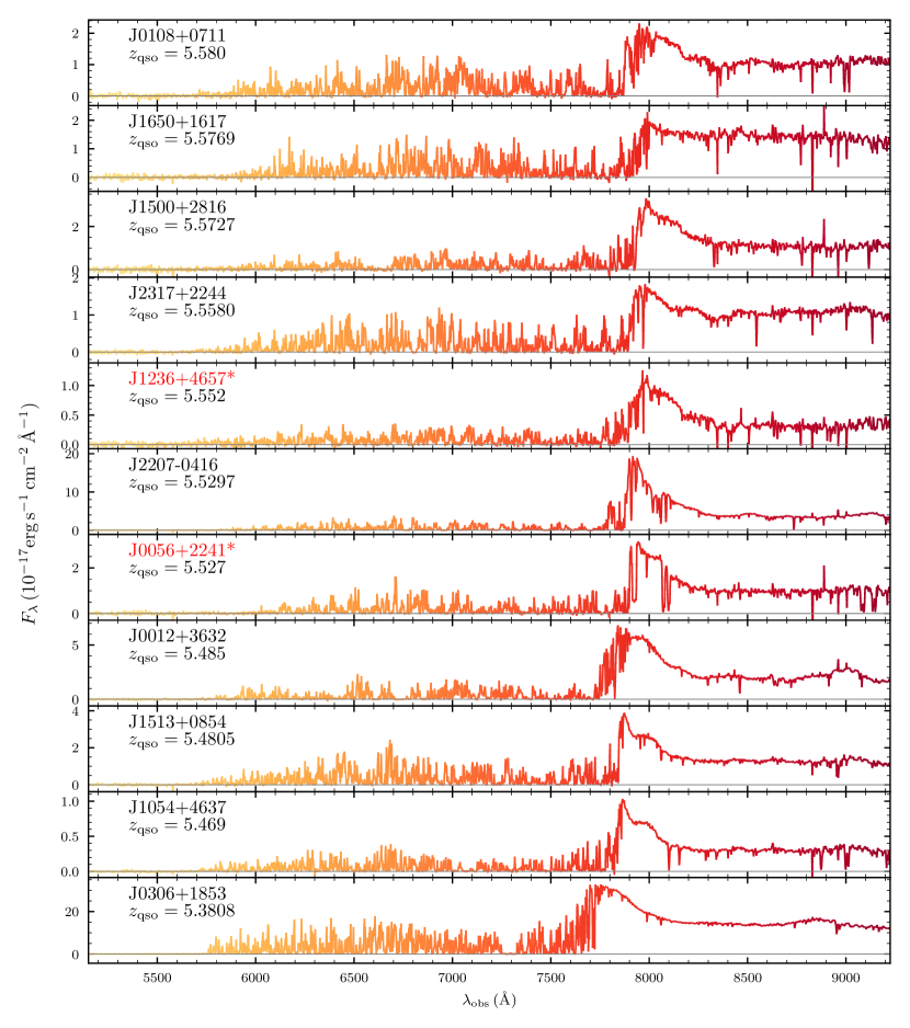
Figure 1: New Keck/ESI QSO spectra obtained for this work. Orange-red and gray curves plot the flux and zero flux, respectively. J0056$+$2241 and J1236$+$4657 (labelled with *) are not included in our sample of $\lambda_{\rm mfp}$ measurements (see text for details). The spectra are re-binned to 2 Å for display.

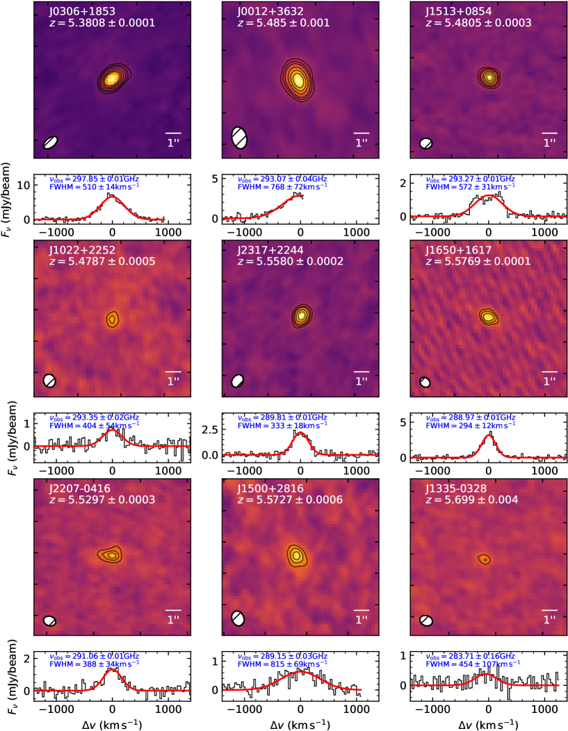
Figure 2: [C II] 158$\mu$m emission maps and spectra of QSOs with our new Keck/ESI observations. Contours show (2$\sigma$, 3$\sigma$, 4$\sigma$, 6$\sigma$, 8$\sigma$, 10$\sigma$) levels. Measured redshifts are labelled for each QSO and red curves show the best Gaussian fits. Observed frequency and FWHM of the [C II] emission are also provided for reference.

In 2021 and 2022, we targeted bright QSOs with $z$-band magnitude $m_{z}\leq 20$ presented in Yang et al. (2017, 2019) using ESI. With a typical exposure time of $\sim 1-3$ hours and using the $1.00^{\prime\prime}$ and $0.75^{\prime\prime}$ slits, we acquired spectra for 11 objects (Figure 1), including 10 QSOs at $z_{\rm qso}\sim 5.5$ (8 of them are included in our sample; see below) and 1 QSO at a lower redshift for replacing its archival spectrum. We followed Becker et al. (2019) to reduce the data, using a custom pipeline that includes optimal techniques for sky subtraction (Kelson, 2003), one-dimensional spectral extraction (Horne, 1986), and telluric absorption corrections for individual exposures using models based on the atmospheric conditions measured by the Cerro Paranal Advanced Sky Model (Noll et al., 2012; Jones et al., 2013). We extracted the spectra with a pixel size of 15 km s^-1. The typical resolution full width at half maximum (FWHM) is approximately 45 km s^-1.

All targets in our sample were selected without any foreknowledge of the Lyman continuum (LyC) transmission. We include all usable spectra as long as the QSO is free from very strong associated metal absorption and/or associated Ly$\alpha$ damping wing absorption, which may bias the $\lambda_{\rm mfp}$ measurements. We also reject objects with strong broad absorption lines (BALs) near the systemic redshift (see Bischetti et al., 2022 for the XQR-30 spectra). Because the LyC transmission is very weak at $z>5.3$, we only use spectra with a signal-to-noise ratio (SNR) of $\gtrsim 20$ per 30 km s^-1 near 1285 Å in the rest frame. Among the objects with new ESI spectra, we exclude J0056 due to its strong associated absorber, and J1236 for its low SNR.

For QSO redshifts, we employ measurements based on sub-millimeter observations, whenever available. Additionally, we carried out ALMA Band 7 observations of our new ESI targets in Cycle 9 and determined the systemic redshifts by fitting the [C II] 158$\mu$m line. For each object, we used two overlapping spectral windows to cover the [C II] line based on the estimated redshift and another two spectral windows to cover the dust continuum. With C43-(1, 2, 3) configurations, the typical angular resolution is $\sim 1^{\prime\prime}$. The data are calibrated and reduced using the default procedures of the CASA pipeline (version 6.4.1.12; McMullin et al., 2007; CASA Team et al., 2022). We follow the procedures described in Eilers et al. (2020) to generate the data cube and image the [C II] line: the [C II] emission is continuum subtracted with uvconstsub, and imaged with the tclean procedure using Briggs cleaning and a robust parameter of 2 (natural weighting) to maximize the sensitivity. We use a robust parameter of 0.5 for J1650+1617 to achieve a best data product. The mean RMS noise of our data set is 0.25 ${\rm mJy\,beam^{-1}}$ per 30 MHz bin. Figure 2 displays [C II] maps along with Gaussian fits to the emission. For each QSO, we extract the spectrum within one beam size centered at the target. We create the [C II] map by stacking the data cube within 1 standard deviation of the Gaussian fit from the line center. We note that the emission line of J0012$+$3632 is incomplete because the [C II] line is at the edge of our spectral window, which was chosen based on a preliminary redshift estimate (Yang et al., 2019). J1513$+$0854 shows a double-peak emission line, which may be due to the rotating disk of the QSO host galaxy. Future observations with higher spatial resolution may help resolve the disk.

For the rest of our sample, we employ redshifts measured from the apparent start of the Ly$\alpha$ forest, which are determined for each line of sight by visually searching for the first Ly$\alpha$ absorption line blueward the Ly$\alpha$ peak (e.g., Worseck et al., 2014; Becker et al., 2019). We do not use redshifts measured from Mg II emission because of their large offsets ($\sim$ 500 km s^-1) from the systemic redshifts (e.g., Venemans et al., 2016; Mazzucchelli et al., 2017; Schindler et al., 2020). Based on 42 QSOs at $5.3<z_{\rm qso}<6.6$ with [C II] or CO redshifts, we find that the redshifts we measure from the apparent start of the Ly$\alpha$ forest are blueshifted from the [C II] or CO redshifts by $\sim 185$ km s^-1 on average, with a standard deviation of $\sim 370$ km s^-1. Such a redshift offset can be explained by the strong proximity zone effect close to the QSO: the first significant absorber may typically occur slightly blueward of the QSO redshift due to ionization effects. This offset is also consistent with that measured in B21. Thus, we shift redshifts measured from the apparent start of the Ly$\alpha$ forest by $+185$ km s^-1 when measuring $\lambda_{\rm mfp}$, and the corrected values are listed in Table 2.

We generate rest-frame composite spectra for QSOs in each $\Delta z=0.3$ bin, starting from $z=4.9$. The redshift bins with a mean redshift of $\langle z\rangle=5.08$, 5.31, 5.65, and 5.93 consist of 44, 26, 9, and 18 spectra, respectively. Following B21, each spectrum is shifted to rest-frame wavelength before being normalized. The normalization is done by dividing each spectrum by its continuum flux measured over wavelengths in the rest frame where the flux from broad emission lines is minimal. Here, we use the continuum flux over $1270{\rm\AA}<\lambda<1380{\rm\AA}$ in the rest frame. We have tested that using a different wavelength window does not significantly change our results. Additionally, we identify and mask wavelength regions affected by skyline subtraction residuals. To reject spurious bad pixels, we apply a light median filter using a 3-pixel sliding window. Mean composite spectra are then computed in 120 km s^-1 bins (as shown in the left-hand panel of Figure 3).

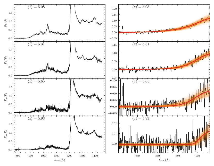
Figure 3: Composite QSO spectra for each redshift bin (left-hand panel) and fits to the LyC transmission (right-hand panel). Black curves show observed flux normalized by the median flux over 1270-1380 Å in the rest frame. The red curve shows our best-fit model. Thin orange curves show the fits from bootstrap realization (only 1000 curves are plotted here for display).

3 Methods

We measure the $\lambda_{\rm mfp}$, which is defined as the distance travelled by ionizing photons that would be attenuated by a factor of $1/e$ by LyC absorption, by fitting the transmitted flux profile blueward of the Lyman limit in composite QSO spectra (Prochaska et al., 2009; B21, ). One challenge with this approach is that the LyC transmission at $z>5$ can be significantly affected by the QSO proximity effect. The ionizing flux from the QSO decreases the ionizing opacity in the proximity zone, which can bias the inferred $\lambda_{\rm mfp}$ high by a factor of two or more (D’Aloisio et al., 2018; B21, ). This is especially important when $\lambda_{\rm mfp}$ is smaller than the proximity zone size, which is true for bright QSOs at $z\gtrsim 5$.

To address this bias, we follow the methods and modeling presented in B21, which modified the Prochaska et al. (2009) method of measuring $\lambda_{\rm mfp}$ to explicitly include the proximity effect. Motivated by simulations, we account for the decrease in ionizing opacity near the QSO by scaling the opacity, $\kappa_{\rm LL}$, according to the local photoionization rate, $\Gamma$. This dependence is modeled as a power law such that $\kappa_{\rm LL}\propto\Gamma^{-\xi}$,

$$\kappa_{\rm LL}(r)=\kappa_{\rm LL}^{\rm bg}\left[1+\frac{\Gamma_{\rm qso}(r)}{\Gamma_{\rm bg}}\right]^{-\xi}~{},$$ (1)

where $\Gamma_{\rm qso}(r)$ is the photoionization rate due to the QSO at a distance $r$ from the QSO, and $\Gamma_{\rm bg}$ is the background photoionization rate. In order to calculate $\Gamma_{\rm qso}(r)$, a key parameter used to describe the proximity zone effect in B21 is $R_{\rm eq}$. It denotes the distance from the QSO where $\Gamma_{\rm qso}(r)$ and $\Gamma_{\rm bg}$ would be equal for purely geometric dilution in the absence of attenuation. Following Calverley et al. (2011), $R_{\rm eq}$ is related to $\Gamma_{\rm bg}$ and the ionizing luminosity of the QSO, $L_{912}$, by

$$R_{\rm eq}=\left[\frac{L_{912}\sigma_{0}}{8\pi^{2}\hbar\Gamma_{\rm bg}(\alpha_{\nu}^{\rm ion}+2.75)}\right]^{1/2}~{},$$ (2)

where $\sigma_{0}$ and $\alpha_{\nu}^{\rm ion}$ are the HI ionization cross section at 912 Å and the power-law index of the QSO continuum at $\lambda<912$ Å in the frequency domain, respectively, and $\hbar$ is the reduced Planck constant. $L_{912}$ can be further related to the absolute magnitude corresponding the the mean luminosity at rest-frame 1450 Å, $L_{1450}$, by $L_{912}=L_{1450}(\nu_{912}/\nu_{1450})^{-\alpha_{\nu}^{\rm UV}}$. Here, $\nu_{912}$ and $\nu_{1450}$ are the photon frequencies at 912 Å and 1450 Å, respectively, and $\alpha_{\nu}^{\rm UV}$ is the power-law slope for the non-ionizing ($912\rm\AA<\lambda<1450\AA$) continuum of the QSO continuum. Following B21, we adopt $\alpha_{\nu}^{\rm ion}=1.5\pm 0.3$ (Telfer et al., 2002; Stevans et al., 2014; Lusso et al., 2015) and $\alpha_{\nu}^{\rm UV}=0.6\pm 0.1$ (Lusso et al., 2015, see also Vanden Berk et al., 2001; Shull et al., 2012; Stevans et al., 2014).

Following B21, the observed flux, $f_{\lambda}^{\rm obs}$, is given by the mean intrinsic QSO continuum, $f_{\lambda}^{\rm cont}\propto(\lambda/912\rm\AA)^{\alpha_{\lambda}^{\rm ion}}$, attenuated by the effective opacity of the Lyman series in the foreground IGM, and the LyC optical depth. The foreground Lyman series opacity is calculated by

$$\tau_{\rm eff}^{\rm Lyman}(\lambda_{\rm obs})=\sum_{j=\rm Ly\alpha,\,Ly\beta,\,...,\,Ly40}\tau_{\rm eff}^{j}(z_{j})\,,$$ (3)

where $\tau_{\rm eff}^{j}(z_{j})$ is the effective opacity of transition $j$ at redshift $z_{j}$ such that $(1+z_{j})\lambda_{j}=\lambda_{\rm obs}$, and $\lambda_{j}$ is the wavelength of transition $j$ in the rest frame. To implement this, we utilized Sherwood simulations (Bolton et al., 2017) to determine the effective optical depth for each Lyman series line across a range of absorption redshifts and $\Gamma$ values. We then include the proximity zone effect for each Lyman series line by matching the effective optical depth to a $\Gamma$ value that corresponds to $\Gamma_{\rm bg}+\Gamma_{\rm qso}$ as a function of distance from the QSO. We compute $\Gamma_{\rm qso}$ by dividing the line of sight into small steps of distance $\delta r$, and solving for $\Gamma_{\rm qso}(r)$ numerically using the method described in B21. For the first step we assume that $\Gamma_{\rm qso}$ decreases purely geometrically, i.e.

$$\Gamma_{\rm qso}(r=\delta r)=\Gamma_{\rm bg}\left(\frac{r}{R_{\rm eq}}\right)^{-2}\,.$$ (4)

We then solve for $\Gamma_{\rm qso}(r+\delta r)$ over subsequent steps as

$$\Gamma_{\rm qso}(r+\delta r)=\Gamma_{\rm qso}(r)\left(\frac{r+\delta r}{r}\right)^{-2}e^{-\kappa_{\rm LL}(r)\delta r}\,,$$ (5)

where $\kappa_{\rm LL}(r)$ is computed using Equation (1). Finally, $\tau_{\rm eff}^{j}(z_{j})$ and $\tau_{\rm eff}^{\rm Lyman}(\lambda_{\rm obs})$ can be computed for each combination of ($\kappa_{\rm LL}^{\rm bg}$, $\xi$, $z_{\rm qso}$, $R_{\rm eq}$), when fitting to the composite spectra. We have also tested that it does not significantly change the measured $\lambda_{\rm mfp}$ by either stacking the foreground Lyman series transmission based on $z_{\rm qso}$ and $R_{\rm eq}$ of each individual QSO (as in B21), or computing a total foreground Lyman series transmission based on the averaged $z_{\rm qso}$ and $R_{\rm eq}$ in each redshift bin.

We use the same procedures for parameterizing the LyC transmission as outlined in B21. However, we make one modification by employing the recent measurements of $\Gamma_{\rm bg}$ from Gaikwad et al. (2023) that match multiple diagnostics of the IGM from observations to the Ly$\alpha$ forest. For reference, the new estimates are $\Gamma_{\rm bg}\simeq 5\times 10^{-13}\rm s^{-1}$ and $1.5\times 10^{-13}\rm s^{-1}$ at $z=5.1$ and 6.0, respectively, in contrast to $7\times 10^{-13}\rm s^{-1}$ and $3\times 10^{-13}\rm s^{-1}$ utilized in B21. The new $\Gamma_{\rm bg}$ at $z=5.1$ is also consistent with measurements in e.g., D’Aloisio et al. (2018). Moreover, instead of assuming a nominal $\pm 0.15$ dex error in $\Gamma_{\rm bg}$, we propagate the uncertainties in the measurements of $\Gamma_{\rm bg}$ from Gaikwad et al. (2023) into $R_{\rm eq}$. We discuss the effect of $\Gamma_{\rm bg}$ on $\lambda_{\rm mfp}$ in Section 4.2.

We fit the transmission for each composite shown in Figure 3 over 820–912 Å in the rest frame. Following B21, uncertainties in $\lambda_{\rm mfp}$ are estimated using a bootstrap approach wherein we randomly draw QSO spectra with replacement in each redshift bin, and refit the new QSO composites for 10,000 realizations. To account for errors in redshift, we randomly shift the spectrum of each QSO that does not have a sub-mm $z_{\rm qso}$ in redshift following a Gaussian distribution with a standard deviation of 370 km s^-1(see Section 2). We include the zero-point as a free parameter while fitting models to the composite, to account for flux zero-point errors. We also treat the normalization of the LyC profile as a free parameter. We randomly vary $\xi$ by assuming a flat prior over $[0.3,1.0]$. The fits are shown in the right-hand panel of Figure 3.

4 Results and Discussion

4.1 $\lambda_{\rm mfp}$ over $5<z<6$

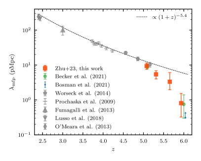
Figure 4: Direct measurements of $\lambda_{\rm mfp}$ from this work (orange-red squares) and from the literature (Becker et al., 2021; Worseck et al., 2014; Prochaska et al., 2009; Fumagalli et al., 2013; Lusso et al., 2018; O’Meara et al., 2013). Error bars show 68% limits. The dashed line shows the power-law extrapolation of $\lambda_{\rm mfp}$ from measurements at $z<5.16$ (Worseck et al., 2014). The blue arrow shows the lower-limit constraint on the $\lambda_{\rm mfp}$ at $z=6$ from Bosman (2021). Symbols are displaced along redshift for display.

Figure 5: (a) Dependence of the $\lambda_{\rm mfp}$ measurements on $\Gamma_{\rm bg}$ at different redshifts. Nominal values and uncertainties of $\Gamma_{\rm bg}$ we adopt from Gaikwad et al. (2023) are shown with horizontal error bars. (b) Measured $\lambda_{\rm mfp}$ based on fixed $\xi$ values of 0.33, 0.67, and 1.00. Symbols are displaced along redshift for display.

We measure $\lambda_{\rm mfp}=9.33_{-1.80(2.82)}^{+2.06(3.76)}$, $5.40_{-1.40(2.39)}^{+1.47(2.39)}$, $3.31_{-1.34(2.06)}^{+2.74(4.02)}$, and $0.81_{-0.48(0.68)}^{+0.73(1.22)}$ pMpc at the averaged redshifts $\langle z\rangle=5.08$, 5.31, 5.65, and 5.93, respectively. The errors give 68% (95%) confidence limits. Figure 4 plots our results along with previous direct $\lambda_{\rm mfp}$ measurements from the literature (Prochaska et al., 2009; Fumagalli et al., 2013; O’Meara et al., 2013; Worseck et al., 2014; Lusso et al., 2018, and B21). Our measurements at both redshift ends are highly consistent with those presented in B21. Our findings clearly indicate a rapid evolution in $\lambda_{\rm mfp}$ at $5<z<6$, particularly at $z\geq 5.3$.

We have confirmed that using different redshift binning does not significantly affect our results. As the composite spectrum at $\langle z\rangle=5.65$ includes relatively fewer QSOs, we tested the robustness of our fitting using mock spectra. We created 1000 sets of $N=9$ mock QSO spectra with similar redshifts and $R_{\rm eq}$ as our sample. The mock spectra were based on our modeling of the transmission at $\lambda<912$ Å, with the mean free path randomly spanning a wide parameter space. We performed 1000 fitting realizations to each of these mock spectra sets, and found that the 68% limits at $z=5.65$ could recover the simulated confidence level quite well. In addition, it is worth noting that none of the objects in our sample are identified as young QSOs with extremely small proximity zones (e.g., Eilers et al., 2020; Satyavolu et al., 2023), given that the $\lambda_{\rm mfp}$ values are quite short near $z\sim 6$.

We note that our $\langle z\rangle=5.65$ stack (Figure 3) includes a small amount of transmission near $\lambda_{\rm rest}\sim 880$ Å, even though the flux has been significantly attenuated at $\lambda_{\rm rest}>890$ Å. We have inspected each individual spectrum in this redshift bin and have found potential transmission near this wavelength ($\lambda_{\rm obs}\sim 5800$ Å) only in the ESI spectra, and not in the X-Shooter spectra. This region is at the boundary of two amplifiers of the ESI CCD. It may also be contaminated by scattered light. This feature might therefore be an instrumental issue ; however, it is also possible that the transmission is real, in which case it may indicate a significant variation in the ionizing free paths towards individual spectra. We hope to explore this in a future work. For the uniform $\lambda_{\rm mfp}$ model used here, however, our tests based on mock spectra indicate that this transmission feature does not significantly impact our measurements.

4.2 Error analysis & dependence on $\Gamma_{\rm bg}$ and $\xi$

Table 2: Error analysis for the measured $\lambda_{\rm mfp}$

	$\langle z\rangle=5.08$	$\langle z\rangle=5.31$	$\langle z\rangle=5.65$	$\langle z\rangle=5.93$
Measured $\lambda_{\rm mfp}$	$9.33_{-1.80}^{+2.06}$	$5.40_{-1.40}^{+1.47}$	$3.31_{-1.34}^{+2.74}$	$0.81_{-0.48}^{+0.73}$
Fixed $\Gamma_{\rm bg}$ and $\xi$	$9.33_{-1.83}^{+1.95}$	$5.40_{-1.14}^{+1.23}$	$3.31_{-0.89}^{+2.52}$	$0.81_{-0.34}^{+0.45}$
Varying $\Gamma_{\rm bg}$ only	$9.33_{-0.69}^{+0.43}$	$5.40_{-0.72}^{+0.62}$	$3.31_{-0.99}^{+0.92}$	$0.81_{-0.26}^{+0.21}$
$\xi=0.33$	$10.10_{-1.69}^{+2.07}$	$6.57_{-1.25}^{+1.23}$	$5.02_{-1.32}^{+1.98}$	$1.53_{-0.49}^{+0.59}$
$\xi=0.67$	$9.33_{-1.81}^{+2.10}$	$5.40_{-1.28}^{+1.27}$	$3.31_{-1.26}^{+2.67}$	$0.81_{-0.40}^{+0.60}$
$\xi=1.00$	$8.74_{-1.88}^{+2.18}$	$4.58_{-1.33}^{+1.30}$	$1.89_{-0.77}^{+3.45}$	$0.30_{-0.13}^{+0.66}$

As described in Section 3, we mitigate the bias on $\lambda_{\rm mfp}$ from the QSO proximity effect by modeling its impact on the ionizing opacity. The effect is parameterized by a nominal proximity zone size $R_{\rm eq}$, which specifies the proper distance at which the hydrogen ionization rate due to the QSO would be equal to the background rate in the absence of any attenuation. Therefore, the measured $\lambda_{\rm mfp}$ has some dependence on $R_{\rm eq}$. Notably, the uncertainties in $R_{\rm eq}$ listed in Table 2 primarily emanate from $\Gamma_{\rm bg}$, with the contribution of uncertainty from $\alpha^{\rm UV}$ and $\alpha^{\rm ion}$ being relatively small ($\lesssim 10\%$). The measurements also depend on $\xi$, as suggested by Equation 1.

Here, we have examined various sources of error in our $\lambda_{\rm mfp}$ measurements, including statistical error, error arising from $\Gamma_{\rm bg}$, and error stemming from $\xi$. Specifically, we evaluate the following: (1) the statistical error obtained by bootstrapping the QSO lines of sight while keeping the nominal values of $\Gamma_{\rm bg}$ and $\xi$ fixed, (2) $\lambda_{\rm mfp}$ values derived by varying $\Gamma_{\rm bg}$ while keeping the QSO composite and $\xi$ constant, and (3) $\lambda_{\rm mfp}$ values obtained for different fixed $\xi$. Table 2 summarizes the results. We would like to emphasize that fixing any of the parameters to their nominal value can lead to a slightly altered distribution of the resulting $\lambda_{\rm mfp}$, and consequently, the corresponding 68% limits may not align precisely with those of the main results. In this case, our primary interest lies in understanding the magnitude of the error.

The “Fixed $\Gamma_{\rm bg}$ and $\xi$” row indicates that the magnitude of the statistical error is comparable to the total error across all redshifts. This suggests that the dominant factor contributing to the error in our measurements is statistical fluctuations, encompassing factors such as the limited number of QSO spectra, flux noise, uncertainties in redshifts, and uncertainties in $\alpha_{\nu}^{\rm UV}$ and $\alpha_{\nu}^{\rm ion}$, among others. As shown in the third row, the random fluctuation in $\Gamma_{\rm bg}$ alone have a minor impact on the overall error. Regarding $\xi$, the last three rows indicate that using a lower (upper) value of $\xi$ shifts the $\lambda_{\rm mfp}$ estimates towards higher (lower) face values. This effect is comparable to the statistical fluctuations and is more pronounced at higher redshifts due to the relatively large $R_{\rm eq}$ in comparison to smaller $\lambda_{\rm mfp}$. Thus, uncertainties in $\xi$ also make a significant contribution to our $\lambda_{\rm mfp}$ measurements.

We also explore how our $\lambda_{\rm mfp}$ measurements depend on $\Gamma_{\rm bg}$ and $\xi$ systematically, such that the results can be easily adjusted for future constraints. Figure 5(a) illustrates the dependence of our best-fitting $\lambda_{\rm mfp}$ measurements on a wide range of $\Gamma_{\rm bg}$ values at each redshift. The figure also displays the nominal $\Gamma_{\rm bg}$ values and their uncertainties. The dependence is minimal at $z\leq 5.3$, where $\lambda_{\rm mfp}\propto\Gamma_{\rm bg}^{\sim 0.2}$. At these redshifts, the proximity zone size is smaller or comparable to $\lambda_{\rm mfp}$, and hence, the measurements are not highly sensitive to $\Gamma_{\rm bg}$. At $z\geq 5.6$, however, $R_{\rm eq}$ is similar to or larger than $\lambda_{\rm mfp}$, leading to a stronger dependence, with $\lambda_{\rm mfp}\propto\Gamma_{\rm bg}^{\sim 0.6}$. Nevertheless, if we adopt the higher end of $\Gamma_{\rm bg}=3\times 10^{-13}\rm s^{-1}$ at $z=5.93$, $\lambda_{\rm mfp}$ would only increase to $\sim 1.0$ pMpc. The results would remain consistent with a steady and rapid $\lambda_{\rm mfp}$ evolution with time.

While there might be an enhanced ionizing background due to galaxies clustering near QSOs, recent research suggests this effect is likely secondary to QSO ionization. Davies (2020) found that even the “ghost” proximity effect of QSOs — a large-scale bias in the ionizing photon mean free path caused by QSO radiation — could overwhelm the ionizing contribution from the clustering of nearby galaxies. In recent JWST observations, Kashino et al. (2023) also found that the impact of a QSO’s ionizing radiation often dominates over local galactic sources near the QSO. These studies reinforce that, despite potential $\Gamma_{\rm bg}$ enhancements from galaxy clustering, the QSO’s influence is typically predominant, as adopted in our modeling for the $\lambda_{\rm mfp}$ measurements.

For our main results, following B21, the mean free path is measured based on a uniform distribution of $\xi\in[0.33,1.00]$, and the face value is measured for $\xi=0.67$. As discussed in B21, however, the scaling of $\kappa_{\rm LL}$ with $\Gamma$ is highly uncertain, especially for high redshifts. The scaling can be milder (smaller $\xi$) when neutral islands and/or self-shielding absorbers are present, and steeper (greater $\xi$) when the IGM shows a more uniform photoionization equilibrium (see e.g., D’Aloisio et al., 2020; Furlanetto & Oh, 2005; McQuinn et al., 2011). For reference, Figure 5(b) shows how our measurements vary with fixed $\xi$ values of 0.33, 0.67, and 1.00. The face value and errors are also listed in Table 2. Similar to the dependence on $\Gamma_{\rm bg}$, the measured $\lambda_{\rm mfp}$ becomes more sensitive to $\xi$ as redshift increases, and as the QSO’s proximity effect becomes stronger relative to a smaller $\lambda_{\rm mfp}$. Even with the extreme $\xi$ values discussed in B21, nevertheless, the measurements are still consistent with our main results with the $1\sigma$ error bars, given the current data. Reassuringly, radiative transfer simulations recently developed by Roth et al. (in prep) suggest that the inferred $\lambda_{\rm mfp}$ using our methods only modestly depends ($\lesssim 20-30\%$) on the QSO lifetimes and environments (see also Satyavolu et al. in prep). Future improved realistic reionization models would provide more insights into the scaling relation, especially when reionization is not fully concluded by $z=6$.

4.3 Implication on when reionization ends

Our measurements not only confirm the $\lambda_{\rm mfp}$ values presented in B21 at $z=5.08$ and 5.93, but also depict a clear evolutionary trend over $5<z<6$. The mean free path increases steadily and rapidly with time: $\lambda_{\rm mfp}$ increases by a factor of $\sim 4$ from $z\simeq 6.0$ to $z\simeq 5.6$, and by a factor of $\sim 2$ every $\Delta z=0.3$ from $z\simeq 5.6$ to $z\simeq 5.0$. This evolution carries important implications for the end of reionization.

D’Aloisio et al. (2020) used radiative transfer hydrodynamic simulations to study the expected evolution of the mean free path following reionization. They found that if reionization had ended well before $z=6$ and the IGM had sufficient time to relax hydrodynamically, then the evolution would expected to follow a trend of $\lambda_{\rm mfp}\propto(1+z)^{-5.4}$. This relation, based on a fully ionized IGM with a homogeneous ionizing UVB, is identical to the best-fitting redshift dependence for direct $\lambda_{\rm mfp}$ measurements at $z\leq 5$ (Worseck et al., 2014). However, as shown in Figure 4, this relation significantly overpredicts the measurements by a factor of $\sim 2-10$ over $5.3<z<6.0$. By this comparison, the data disfavor a fully ionized and relaxed IGM with a homogeneous UVB at these redshifts.

One possible explanation for the rapid evolution in $\lambda_{\rm mfp}$ is that reionization ends later than $z=6$. Such a late-ending reionization scenario has recently been proposed to explain large-scale fluctuations in the observed Ly$\alpha$ effective optical depth ($\tau_{\rm eff}$) at $z>5$ (e.g., Kulkarni et al., 2019; Keating et al., 2020b; Nasir & D’Aloisio, 2020; Choudhury et al., 2021; Qin et al., 2021). The rapid evolution in $\lambda_{\rm mfp}$ can be naturally explained by ongoing reionization when large ionized bubbles merge and dense, optically-thick ionization sinks are photo-evaporated (e.g., Furlanetto & Oh, 2005; Sobacchi & Mesinger, 2014; D’Aloisio et al., 2020). As mentioned above, the rapid evolution in $\lambda_{\rm mfp}$ persists as late as $z\lesssim 5.3$, and the significant discrepancy between measurements and predictions from the relaxed IGM model also appears as late as $z=5.3$. Interestingly, the rapid evolution in $\lambda_{\rm mfp}$ appears to coincide in redshift with the appearance of large fluctuations in the observed Ly$\alpha$ $\tau_{\rm eff}$ at $z\gtrsim 5.3$ (e.g., Becker et al., 2015; Eilers et al., 2018; Bosman et al., 2018, 2022; Yang et al., 2020b). This may be due to the fact that a shorter $\lambda_{\rm mfp}$, along with any potential neutral component from incomplete reionization, will boost the fluctuations in the ionizing UV background, producing scatter in $\tau_{\rm eff}$ (e.g., Davies & Furlanetto, 2016; Nasir & D’Aloisio, 2020; Qin et al., 2021). This joint evolution in the mean free path and UV background is expected near the end of reionization (e.g., Kulkarni et al., 2019; Keating et al., 2020b; Nasir & D’Aloisio, 2020). Such a scenario is also consistent with long dark gaps observed in the Ly$\alpha$/Ly$\beta$ forest (Zhu et al., 2021, 2022) at $z<6$, and the fraction of dark pixels measured in the forest (McGreer et al., 2015; Jin et al., 2023).

4.4 Comparison with reionization simulations

Figure 6: (a) Direct measurements of $\lambda_{\rm mfp}$ from this work (orange-red squares) compared to the predictions from recent models (Cain et al., 2021; Garaldi et al., 2022; Lewis et al., 2022). (b) Our measurements compared with indirect constraints based on Ly$\alpha$ opacities (Gaikwad et al., 2023, Davies et al. in prep., Qin et al. in prep.). Open circles correspond to marginal constraints and arrows correspond to $2\sigma$ limits for Davies et al. (in prep). The shaded region shows the posterior from Qin et al. (in prep.) at the 68% confidence level. In both panels, for comparison, we also show the direct $\lambda_{\rm mfp}$ measurements in Becker et al. (2021) and Worseck et al. (2014), as well as the lower-limit constraint in Bosman (2021). Symbols are displaced along redshift for display.

Figure 6(a) compares our $\lambda_{\rm mfp}$ measurements to recent numerical simulations of reionization, including the enhanced-sink simulation in Cain et al. (2021), THESAN in Garaldi et al. (2022), and CoDaIII in Lewis et al. (2022). These models use late-ending reionization histories and aim to explain the observed short $\lambda_{\rm mfp}$ at $z=6$ and the rapid evolution measured in B21, which we have confirmed in finer detail here. We also include the ATON simulation (“low $\tau_{\rm CMB}$” model) in Keating et al. (2020a) for reference.

Cain et al. (2021) reproduce $\lambda_{\rm mfp}$ that is consistent with the $z=6$ measurements in a late-ending reionization driven by faint galaxies. However, they also find that either a rapid drop in emissivity at $z<6$ or extra sinks are required to reproduce the $\lambda_{\rm mfp}$ measurements at $z<5.2$ in this scenario. Garaldi et al. (2022) use a radiative hydrodynamics simulation and generally reproduce the rapid evolution of $\lambda_{\rm mfp}$  although overshoot the $z=6$ measurement. They find that all of their late-reionization simulations can reproduce a dramatic evolution in $\lambda_{\rm mfp}$ from $z=5.5$ to 6, while one simulation wherein reionization ends by $z>6$ cannot. Lewis et al. (2022) also find that reionization ending later than $z<6$ is able to naturally explain the observations, although a drop in the emissivity is required near the end of reionization (Ocvirk et al., 2021).

We note that these simulations measure the $\lambda_{\rm mfp}$ in slightly different manners. Cain et al. (2021) generate mock LyC QSO spectra using randomly placed sightlines, and fit the stacked spectra using the model proposed by Prochaska et al. (2009). This procedure mimics the method used in Worseck et al. (2014). On the other hand, Garaldi et al. (2022) measure the distance at which the LyC transmission is attenuated by a factor of $1/e$ from individual sightlines, and take the average. Finally, Lewis et al. (2022) adopted multiple measurement methods for the $\lambda_{\rm mfp}$, and the curve shown in Figure 6(a) represents the median distance to a $1/e$ attenuation in LyC among sightlines. We also note that the models shown here may not necessarily reproduce observations of the Ly$\alpha$ forest transmission (e.g., Garaldi et al., 2022). Nevertheless, the rapid evolution of $\lambda_{\rm mfp}$ that we measure over $5<z<6$ is broadly consistent with these models that align with a late conclusion to reionization.

4.5 Comparison with constraints on $\lambda_{\rm mfp}$ from Ly$\alpha$ opacities

Recently, Gaikwad et al. (2023) and Davies et al. (in prep) have used alternative methods to probe the evolution of $\lambda_{\rm mfp}$ at these redshifts. Instead of directly measuring $\lambda_{\rm mfp}$ from the LyC transmission, they use inference methods to jointly constrain $\lambda_{\rm mfp}$ and $\Gamma_{\rm bg}$ by modeling the observed Ly$\alpha$ effective optical depth distribution. Specifically, Gaikwad et al. (2023) post-processed hydrodynamic IGM simulations using a fluctuating UV background specified by a spatially-averaged photoionization rate and a mean-free path parameter, $\lambda_{0}$. These variables are constrained by comparing the simulated cumulative distribution function of $\tau_{\rm eff}$ with observations using a non-parametric two-sample Anderson-Darlington test. A value of the physical mean free path, $\lambda_{\rm mfp}$, is then inferred from the simulated neutral hydrogen distribution once the best-fitting UV background is applied. This step is particularly significant at $z\lesssim 5.3$, where the $\tau_{\rm eff}$ distribution is consistent with a uniform UVB (see also Becker et al., 2018; Bosman et al., 2022) and does not constrain $\lambda_{\rm mfp}$ directly. The fact that the constraints at these redshifts from Gaikwad et al. (2023) agree with the direct constrains presented here suggests that their simulations may be modeling much of the ionizing opacity.

Davies et al. (in prep) take a similar approach but use a combination of hydrodynamical and semi-numerical simulations to model the density field, and employ a likelihood-free inference technique of approximate Bayesian computation to constrain $\lambda_{\rm mfp}$ and $\Gamma_{\rm bg}$ based on the Ly$\alpha$ forest observations. Davies et al. (in prep) also constrain $\lambda_{\rm mfp}$ by treating it as an “input” sub-grid parameter for the UVB fluctuations rather than inferring it from a derived H I density distribution. This accounts for the fact that the Davies et al. (in prep) values at $z<5.3$ are lower limits.

As shown in Figure 6(b), these indirect $\lambda_{\rm mfp}$ constraints are generally consistent ($\lesssim 1\sigma$) with the direct measurements presented here and in B21. This suggests that the rapidly evolving $\lambda_{\rm mfp}$ values needed for UV background fluctuations to drive the observed Ly$\alpha$ $\tau_{\rm eff}$ distribution are consistent with the attenuation of ionizing photons we observe directly. We note that Gaikwad et al. (2023) and Davies et al. (in prep) present somewhat different pictures of the IGM at these redshifts; the Gaikwad et al. (2023) models include neutral islands persisting to $z\simeq 5.2$ while Davies et al. (in prep) have the flexibility to vary the $\lambda_{\rm mfp}$ distribution within ionized regions although no neutral islands are explicitly included. These models are broadly consistent with one another in that the Ly$\alpha$ opacity fluctuations are mainly driven by UV background fluctuations, but this difference highlights the range of physical scenarios that are still formally consistent with the data.

We also include the inference based on multiple observations. Recently, Qin et al. (in prep) use the 21cmFAST Epoch of Reionization (EoR) simulations (Mesinger et al., 2011; Murray et al., 2020) to constrain IGM properties including its $\lambda_{\rm mfp}$. Their input parameters represent galaxy properties such as the stellar-to-halo mass ratio, UV escape fraction and duty cycles. These allow them to evaluate the UV ionizing photon budget and forward model the impact on the IGM. Within a Bayesian framework, they include not only the XQR-30 measurement of the forest fluctuations (Bosman et al., 2022) when computing the likelihood but also the CMB optical depth and galaxy UV luminosity functions. Therefore, the posterior they obtain for the IGM mean free path potentially represents a comprehensive constraint from all currently existing EoR observables. As Figure 6(b) displays, the posterior from Qin et al. (in prep) also show a rapid increase in the $\lambda_{\rm mfp}$ with time between $5\lesssim z\lesssim 6$. Although the posterior does not follow the exact trace of our direct measurements, the general consistency may suggest that such a rapid evolution in $\lambda_{\rm mfp}$ is potentially favored by other EoR observables.

5 Conclusion

We have presented new measurements of the ionizing mean free path between $z=5.0$ and $6.0$. These are the first direct measurements in multiple redshift bins over this interval, allowing us to trace the evolution of $\lambda_{\rm mfp}$ near the end of reionization. Our measurements are based on new and archival data, including new Keck/ESI observations and spectra from the XQR-30 program. By fitting the LyC transmission in composite spectra, we report $\lambda_{\rm mfp}$= $9.33_{-1.80}^{+2.06}$, $5.40_{-1.40}^{+1.47}$, $3.31_{-1.34}^{+2.74}$, and $0.81_{-0.48}^{+0.73}$ pMpc, at $\langle z\rangle=5.08$, 5.31, 5.65, and 5.93, respectively. The results confirm the dramatic evolution in $\lambda_{\rm mfp}$ over $5<z<6$, as first reported in B21, and further show a steady and rapid evolution, with a factor of $\sim 4$ increase from $z\simeq 6.0$ to $z\simeq 5.6$, and a factor of $\sim 2$ increase every $\Delta z=0.3$ from $z\simeq 5.6$ to $z\simeq 5.0$. Our $\lambda_{\rm mfp}$ measurements disfavor a fully ionized and relaxed IGM with a homogeneous UVB at $\gtrsim 95\%$ confidence level down to at least $z\sim 5.3$ and are coincident with the onset of the fluctuations in observed $\tau_{\rm eff}$ at $z\sim 5.3$.

Recent indirect $\lambda_{\rm mfp}$ constraints based on IGM Ly$\alpha$ opacity from Gaikwad et al. (2023) and Davies et al. (in prep) agree well with our measurements and those in B21. Our results are also broadly consistent with a range of late-ending reionization models (Cain et al., 2021; Garaldi et al., 2022; Lewis et al., 2022; Gaikwad et al., 2023). Along with other probes from the Ly$\alpha$ and Ly$\beta$ forests, our results suggest that islands of neutral gas and/or large fluctuations in the UV background may persist in the IGM well below redshift six.

References

- Astropy Collaboration et al. (2013) Astropy Collaboration, Robitaille, T. P., Tollerud, E. J., et al. 2013, A&A, 558, A33, doi: 10.1051/0004-6361/201322068
- Bañados et al. (2016) Bañados, E., Venemans, B. P., Decarli, R., et al. 2016, The Astrophysical Journal Supplement Series, 227, 11, doi: 10.3847/0067-0049/227/1/11
- Bañados et al. (2018) Bañados, E., Venemans, B. P., Mazzucchelli, C., et al. 2018, Nature, 553, 473, doi: 10.1038/nature25180
- Bañados et al. (2023) Bañados, E., Schindler, J.-T., Venemans, B. P., et al. 2023, The Astrophysical Journal Supplement Series, 265, 29, doi: 10.3847/1538-4365/acb3c7
- Becker et al. (2015) Becker, G. D., Bolton, J. S., Madau, P., et al. 2015, MNRAS, 447, 3402, doi: 10.1093/mnras/stu2646
- Becker et al. (2021) Becker, G. D., D’Aloisio, A., Christenson, H. M., et al. 2021, MNRAS, 508, 1853, doi: 10.1093/mnras/stab2696
- Becker et al. (2018) Becker, G. D., Davies, F. B., Furlanetto, S. R., et al. 2018, ApJ, 863, 92, doi: 10.3847/1538-4357/aacc73
- Becker et al. (2019) Becker, G. D., Pettini, M., Rafelski, M., et al. 2019, ApJ, 883, 163, doi: 10.3847/1538-4357/ab3eb5
- Bezanson et al. (2015) Bezanson, J., Edelman, A., Karpinski, S., & Shah, V. B. 2015, Julia: A Fresh Approach to Numerical Computing, arXiv. http://ascl.net/1411.1607
- Bischetti et al. (2022) Bischetti, M., Feruglio, C., D’Odorico, V., et al. 2022, Nature, 605, 244, doi: 10.1038/s41586-022-04608-1
- Boera et al. (2019) Boera, E., Becker, G. D., Bolton, J. S., & Nasir, F. 2019, ApJ, 872, 101, doi: 10.3847/1538-4357/aafee4
- Bolton et al. (2017) Bolton, J. S., Puchwein, E., Sijacki, D., et al. 2017, MNRAS, 464, 897, doi: 10.1093/mnras/stw2397
- Bosman (2021) Bosman, S. E. I. 2021, Constraints on the Mean Free Path of Ionising Photons at $z\sim6$ Using Limits on Individual Free Paths, doi: 10.48550/arXiv.2108.12446
- Bosman et al. (2018) Bosman, S. E. I., Fan, X., Jiang, L., et al. 2018, MNRAS, 479, 1055, doi: 10.1093/mnras/sty1344
- Bosman et al. (2022) Bosman, S. E. I., Davies, F. B., Becker, G. D., et al. 2022, MNRAS, 514, 55, doi: 10.1093/mnras/stac1046
- Cain et al. (2021) Cain, C., D’Aloisio, A., Gangolli, N., & Becker, G. D. 2021, ApJ, 917, L37, doi: 10.3847/2041-8213/ac1ace
- Calverley et al. (2011) Calverley, A. P., Becker, G. D., Haehnelt, M. G., & Bolton, J. S. 2011, MNRAS, 412, 2543, doi: 10.1111/j.1365-2966.2010.18072.x
- Carilli et al. (2007) Carilli, C. L., Neri, R., Wang, R., et al. 2007, ApJ, 666, L9, doi: 10.1086/521648
- Carnall (2017) Carnall, A. C. 2017, arXiv e-prints, arXiv:1705.05165
- CASA Team et al. (2022) CASA Team, Bean, B., Bhatnagar, S., et al. 2022, PASP, 134, 114501, doi: 10.1088/1538-3873/ac9642
- Chen et al. (2022) Chen, H., Eilers, A.-C., Bosman, S. E. I., et al. 2022, ApJ, 931, 29, doi: 10.3847/1538-4357/ac658d
- Choudhury et al. (2021) Choudhury, T. R., Paranjape, A., & Bosman, S. E. I. 2021, MNRAS, 501, 5782, doi: 10.1093/mnras/stab045
- Christenson et al. (2021) Christenson, H. M., Becker, G. D., Furlanetto, S. R., et al. 2021, ApJ, 923, 87, doi: 10.3847/1538-4357/ac2a34
- Coulais et al. (2014) Coulais, A., Schellens, M., Duvert, G., et al. 2014, 485, 331
- D’Aloisio et al. (2018) D’Aloisio, A., McQuinn, M., Davies, F. B., & Furlanetto, S. R. 2018, MNRAS, 473, 560, doi: 10.1093/mnras/stx2341
- D’Aloisio et al. (2020) D’Aloisio, A., McQuinn, M., Trac, H., Cain, C., & Mesinger, A. 2020, ApJ, 898, 149, doi: 10.3847/1538-4357/ab9f2f
- Davies (2020) Davies, F. B. 2020, MNRAS, 494, 2937, doi: 10.1093/mnras/staa528
- Davies et al. (2021) Davies, F. B., Bosman, S. E. I., Furlanetto, S. R., Becker, G. D., & D’Aloisio, A. 2021, ApJ, 918, L35, doi: 10.3847/2041-8213/ac1ffb
- Davies & Furlanetto (2016) Davies, F. B., & Furlanetto, S. R. 2016, MNRAS, 460, 1328, doi: 10.1093/mnras/stw931
- Davies et al. (2018) Davies, F. B., Hennawi, J. F., Bañados, E., et al. 2018, ApJ, 864, 142, doi: 10.3847/1538-4357/aad6dc
- Davies et al. (2023a) Davies, R. L., Ryan-Weber, E., D’Odorico, V., et al. 2023a, MNRAS, 521, 289, doi: 10.1093/mnras/stac3662
- Davies et al. (2023b) —. 2023b, MNRAS, 521, 314, doi: 10.1093/mnras/stad294
- de Belsunce et al. (2021) de Belsunce, R., Gratton, S., Coulton, W., & Efstathiou, G. 2021, MNRAS, 507, 1072, doi: 10.1093/mnras/stab2215
- Decarli et al. (2018) Decarli, R., Walter, F., Venemans, B. P., et al. 2018, ApJ, 854, 97, doi: 10.3847/1538-4357/aaa5aa
- D’Odorico et al. (2023) D’Odorico, V., Banados, E., Becker, G. D., et al. 2023, XQR-30: The Ultimate XSHOOTER Quasar Sample at the Reionization Epoch, doi: 10.48550/arXiv.2305.05053
- Eilers et al. (2018) Eilers, A.-C., Davies, F. B., & Hennawi, J. F. 2018, ApJ, 864, 53, doi: 10.3847/1538-4357/aad4fd
- Eilers et al. (2020) Eilers, A.-C., Hennawi, J. F., Decarli, R., et al. 2020, ApJ, 900, 37, doi: 10.3847/1538-4357/aba52e
- Fan et al. (2006) Fan, X., Strauss, M. A., Becker, R. H., et al. 2006, AJ, 132, 117, doi: 10.1086/504836
- Farina et al. (2019) Farina, E. P., Arrigoni-Battaia, F., Costa, T., et al. 2019, ApJ, 887, 196, doi: 10.3847/1538-4357/ab5847
- Fumagalli et al. (2013) Fumagalli, M., O’Meara, J. M., Prochaska, J. X., & Worseck, G. 2013, ApJ, 775, 78, doi: 10.1088/0004-637X/775/1/78
- Furlanetto & Oh (2005) Furlanetto, S. R., & Oh, S. P. 2005, MNRAS, 363, 1031, doi: 10.1111/j.1365-2966.2005.09505.x
- Gaikwad et al. (2021) Gaikwad, P., Srianand, R., Haehnelt, M. G., & Choudhury, T. R. 2021, MNRAS, 506, 4389, doi: 10.1093/mnras/stab2017
- Gaikwad et al. (2023) Gaikwad, P., Haehnelt, M. G., Davies, F. B., et al. 2023, Measuring the Photo-Ionization Rate, Neutral Fraction and Mean Free Path of HI Ionizing Photons at $4.9 \leq z \leq 6.0$ from a Large Sample of XShooter and ESI Spectra, arXiv. http://ascl.net/2304.02038
- Garaldi et al. (2022) Garaldi, E., Kannan, R., Smith, A., et al. 2022, MNRAS, 512, 4909, doi: 10.1093/mnras/stac257
- Greig et al. (2021) Greig, B., Mesinger, A., Davies, F. B., et al. 2021, arXiv:2112.04091. http://ascl.net/2112.04091
- Hoag et al. (2019) Hoag, A., Bradač, M., Huang, K., et al. 2019, ApJ, 878, 12, doi: 10.3847/1538-4357/ab1de7
- Horne (1986) Horne, K. 1986, PASP, 98, 609, doi: 10.1086/131801
- Hu et al. (2019) Hu, W., Wang, J., Zheng, Z.-Y., et al. 2019, ApJ, 886, 90, doi: 10.3847/1538-4357/ab4cf4
- Hunter (2007) Hunter, J. D. 2007, CSE, 9, 90, doi: 10.1109/MCSE.2007.55
- Jin et al. (2023) Jin, X., Yang, J., Fan, X., et al. 2023, ApJ, 942, 59, doi: 10.3847/1538-4357/aca678
- Jones et al. (2013) Jones, A., Noll, S., Kausch, W., Szyszka, C., & Kimeswenger, S. 2013, A&A, 560, A91, doi: 10.1051/0004-6361/201322433
- Jung et al. (2020) Jung, I., Finkelstein, S. L., Dickinson, M., et al. 2020, ApJ, 904, 144, doi: 10.3847/1538-4357/abbd44
- Kashino et al. (2023) Kashino, D., Lilly, S. J., Matthee, J., et al. 2023, ApJ, 950, 66, doi: 10.3847/1538-4357/acc588
- Kashino et al. (2020) Kashino, D., Lilly, S. J., Shibuya, T., Ouchi, M., & Kashikawa, N. 2020, ApJ, 888, 6, doi: 10.3847/1538-4357/ab5a7d
- Keating et al. (2020a) Keating, L. C., Kulkarni, G., Haehnelt, M. G., Chardin, J., & Aubert, D. 2020a, MNRAS, 497, 906, doi: 10.1093/mnras/staa1909
- Keating et al. (2020b) Keating, L. C., Weinberger, L. H., Kulkarni, G., et al. 2020b, MNRAS, 491, 1736, doi: 10.1093/mnras/stz3083
- Kelson (2003) Kelson, D. D. 2003, PASP, 115, 688, doi: 10.1086/375502
- Kulkarni et al. (2019) Kulkarni, G., Keating, L. C., Haehnelt, M. G., et al. 2019, MNRAS, 485, L24, doi: 10.1093/mnrasl/slz025
- Lai et al. (2022) Lai, S., Bian, F., Onken, C. A., et al. 2022, MNRAS, 513, 1801, doi: 10.1093/mnras/stac1001
- Lewis et al. (2022) Lewis, J. S. W., Ocvirk, P., Sorce, J. G., et al. 2022, MNRAS, 516, 3389, doi: 10.1093/mnras/stac2383
- Lusso et al. (2018) Lusso, E., Fumagalli, M., Rafelski, M., et al. 2018, ApJ, 860, 41, doi: 10.3847/1538-4357/aac514
- Lusso et al. (2015) Lusso, E., Worseck, G., Hennawi, J. F., et al. 2015, MNRAS, 449, 4204, doi: 10.1093/mnras/stv516
- Mason et al. (2018) Mason, C. A., Treu, T., Dijkstra, M., et al. 2018, ApJ, 856, 2, doi: 10.3847/1538-4357/aab0a7
- Mason et al. (2019) Mason, C. A., Fontana, A., Treu, T., et al. 2019, MNRAS, 485, 3947, doi: 10.1093/mnras/stz632
- Mazzucchelli et al. (2017) Mazzucchelli, C., Bañados, E., Venemans, B. P., et al. 2017, ApJ, 849, 91, doi: 10.3847/1538-4357/aa9185
- McGreer et al. (2018) McGreer, I. D., Fan, X., Jiang, L., & Cai, Z. 2018, AJ, 155, 131, doi: 10.3847/1538-3881/aaaab4
- McGreer et al. (2015) McGreer, I. D., Mesinger, A., & D’Odorico, V. 2015, MNRAS, 447, 499, doi: 10.1093/mnras/stu2449
- McGreer et al. (2013) McGreer, I. D., Jiang, L., Fan, X., et al. 2013, ApJ, 768, 105, doi: 10.1088/0004-637X/768/2/105
- McMullin et al. (2007) McMullin, J. P., Waters, B., Schiebel, D., Young, W., & Golap, K. 2007, 376, 127
- McQuinn et al. (2011) McQuinn, M., Oh, S. P., & Faucher-Giguère, C.-A. 2011, ApJ, 743, 82, doi: 10.1088/0004-637X/743/1/82
- Mesinger et al. (2011) Mesinger, A., Furlanetto, S., & Cen, R. 2011, MNRAS, 411, 955, doi: 10.1111/j.1365-2966.2010.17731.x
- Murray et al. (2020) Murray, S., Greig, B., Mesinger, A., et al. 2020, The Journal of Open Source Software, 5, 2582, doi: 10.21105/joss.02582
- Nasir & D’Aloisio (2020) Nasir, F., & D’Aloisio, A. 2020, MNRAS, 494, 3080, doi: 10.1093/mnras/staa894
- Noll et al. (2012) Noll, S., Kausch, W., Barden, M., et al. 2012, A&A, 543, A92, doi: 10.1051/0004-6361/201219040
- Ocvirk et al. (2021) Ocvirk, P., Lewis, J. S. W., Gillet, N., et al. 2021, MNRAS, 507, 6108, doi: 10.1093/mnras/stab2502
- O’Meara et al. (2013) O’Meara, J. M., Prochaska, J. X., Worseck, G., Chen, H.-W., & Madau, P. 2013, ApJ, 765, 137, doi: 10.1088/0004-637X/765/2/137
- Park et al. (2016) Park, H., Shapiro, P. R., Choi, J.-h., et al. 2016, ApJ, 831, 86, doi: 10.3847/0004-637X/831/1/86
- Planck Collaboration et al. (2020) Planck Collaboration, Aghanim, N., Akrami, Y., et al. 2020, A&A, 641, A6, doi: 10.1051/0004-6361/201833910
- Prochaska et al. (2003) Prochaska, J. X., Gawiser, E., Wolfe, A. M., Cooke, J., & Gelino, D. 2003, The Astrophysical Journal Supplement Series, 147, 227, doi: 10.1086/375839
- Prochaska et al. (2009) Prochaska, J. X., Worseck, G., & O’Meara, J. M. 2009, ApJ, 705, L113, doi: 10.1088/0004-637X/705/2/L113
- Qin et al. (2021) Qin, Y., Mesinger, A., Bosman, S. E. I., & Viel, M. 2021, arXiv e-prints, 2101, arXiv:2101.09033. http://ascl.net/2101.09033
- Satyavolu et al. (2023) Satyavolu, S., Eilers, A.-C., Kulkarni, G., et al. 2023, MNRAS, 522, 4918, doi: 10.1093/mnras/stad1326
- Schindler et al. (2020) Schindler, J.-T., Farina, E. P., Bañados, E., et al. 2020, ApJ, 905, 51, doi: 10.3847/1538-4357/abc2d7
- Shapiro et al. (2004) Shapiro, P. R., Iliev, I. T., & Raga, A. C. 2004, MNRAS, 348, 753, doi: 10.1111/j.1365-2966.2004.07364.x
- Sheinis et al. (2002) Sheinis, A. I., Bolte, M., Epps, H. W., et al. 2002, PASP, 114, 851, doi: 10.1086/341706
- Shull et al. (2012) Shull, J. M., Stevans, M., & Danforth, C. W. 2012, ApJ, 752, 162, doi: 10.1088/0004-637X/752/2/162
- Sobacchi & Mesinger (2014) Sobacchi, E., & Mesinger, A. 2014, MNRAS, 440, 1662, doi: 10.1093/mnras/stu377
- Stevans et al. (2014) Stevans, M. L., Shull, J. M., Danforth, C. W., & Tilton, E. M. 2014, ApJ, 794, 75, doi: 10.1088/0004-637X/794/1/75
- Telfer et al. (2002) Telfer, R. C., Zheng, W., Kriss, G. A., & Davidsen, A. F. 2002, ApJ, 565, 773, doi: 10.1086/324689
- van der Walt et al. (2011) van der Walt, S., Colbert, S. C., & Varoquaux, G. 2011, CSE, 13, 22, doi: 10.1109/MCSE.2011.37
- Vanden Berk et al. (2001) Vanden Berk, D. E., Richards, G. T., Bauer, A., et al. 2001, AJ, 122, 549, doi: 10.1086/321167
- Venemans et al. (2016) Venemans, B. P., Walter, F., Zschaechner, L., et al. 2016, ApJ, 816, 37, doi: 10.3847/0004-637X/816/1/37
- Venemans et al. (2020) Venemans, B. P., Walter, F., Neeleman, M., et al. 2020, ApJ, 904, 130, doi: 10.3847/1538-4357/abc563
- Vernet et al. (2011) Vernet, J., Dekker, H., D’Odorico, S., et al. 2011, A&A, 536, A105, doi: 10.1051/0004-6361/201117752
- Wang et al. (2016) Wang, F., Wu, X.-B., Fan, X., et al. 2016, ApJ, 819, 24, doi: 10.3847/0004-637X/819/1/24
- Wang et al. (2020) Wang, F., Davies, F. B., Yang, J., et al. 2020, ApJ, 896, 23, doi: 10.3847/1538-4357/ab8c45
- Wang et al. (2010) Wang, R., Carilli, C. L., Neri, R., et al. 2010, ApJ, 714, 699, doi: 10.1088/0004-637X/714/1/699
- Wang et al. (2013) Wang, R., Wagg, J., Carilli, C. L., et al. 2013, ApJ, 773, 44, doi: 10.1088/0004-637X/773/1/44
- Weinberger et al. (2019) Weinberger, L. H., Haehnelt, M. G., & Kulkarni, G. 2019, MNRAS, 485, 1350, doi: 10.1093/mnras/stz481
- Wold et al. (2021) Wold, I. G. B., Malhotra, S., Rhoads, J., et al. 2021, arXiv e-prints, arXiv:2105.12191
- Worseck et al. (2014) Worseck, G., Prochaska, J. X., O’Meara, J. M., et al. 2014, MNRAS, 445, 1745, doi: 10.1093/mnras/stu1827
- Yang et al. (2017) Yang, J., Fan, X., Wu, X.-B., et al. 2017, AJ, 153, 184, doi: 10.3847/1538-3881/aa6577
- Yang et al. (2019) Yang, J., Wang, F., Fan, X., et al. 2019, ApJ, 871, 199, doi: 10.3847/1538-4357/aaf858
- Yang et al. (2020a) —. 2020a, ApJ, 897, L14, doi: 10.3847/2041-8213/ab9c26
- Yang et al. (2020b) —. 2020b, ApJ, 904, 26, doi: 10.3847/1538-4357/abbc1b
- Zhu et al. (2021) Zhu, Y., Becker, G. D., Bosman, S. E. I., et al. 2021, ApJ, 923, 223, doi: 10.3847/1538-4357/ac26c2
- Zhu et al. (2022) —. 2022, ApJ, 932, 76, doi: 10.3847/1538-4357/ac6e60