Meta-Learning Operators to Optimality from Multi-Task Non-IID Data

Abstract

A powerful concept behind much of the recent progress in machine learning is the extraction of common features across data from heterogeneous sources or tasks. Intuitively, using all of one’s data to learn a common representation function benefits both computational effort and statistical generalization by leaving a smaller number of parameters to fine-tune on a given task. Toward theoretically grounding these merits, we propose a general setting of recovering linear operators $M$ from noisy vector measurements $y=Mx+w$, where the covariates $x$ may be both non-i.i.d. and non-isotropic. We demonstrate that existing isotropy-agnostic meta-learning approaches incur biases on the representation update, which causes the scaling of the noise terms to lose favorable dependence on the number of source tasks. This in turn can cause the sample complexity of representation learning to be bottlenecked by the single-task data size. We introduce an adaptation, De-bias & Feature-Whiten (DFW), of the popular alternating minimization-descent (AMD) scheme proposed in [1], and establish linear convergence to the optimal representation with noise level scaling down with the total source data size. This leads to generalization bounds on the same order as an oracle empirical risk minimizer. We verify the vital importance of DFW on various numerical simulations. In particular, we show that vanilla alternating-minimization descent fails catastrophically even for iid, but mildly non-isotropic data. Our analysis unifies and generalizes prior work, and provides a flexible framework for a wider range of applications, such as in controls and dynamical systems.

1 Introduction

A unifying paradigm belying recent exciting progress in machine learning is learning a common feature space or representation for downstream tasks from heterogeneous sources. This forms the core of fields such as meta-learning, transfer learning, and federated learning. A shared theme across these fields is the scarcity of data for a specific task out of many, such that designing individual models for each task is both computationally and statistically inefficient, impractical, or impossible. Under the assumption that these tasks are similar in some way, a natural alternative approach is to use data across many tasks to learn a common component, such that fine-tuning to a given task involves fitting a much smaller model that acts on the common component. Over the last few years, significant attention has been given to framing this problem setting theoretically, providing provable benefits of learning over multiple tasks in the context of linear regression [2, 3, 4, 1, 5, 6] and in identification/control of linear dynamical systems [7, 8, 9]. These works study the problem of linear representation learning, where the data for each task is generated noisily from an unknown shared latent subspace, and the goal is to efficiently recover a representation of the latent space $\hat{\Phi}$ from data across different task distributions. For example, in the linear regression setting, one may have data of the form

$$\mathopen{}y^{(h)}_{i}\mathclose{}={\theta^{(h)}}^{\top}\Phi\mathopen{}x^{(h)}_{i}\mathclose{}+\mathrm{noise},\quad\mathopen{}y^{(h)}_{i}\mathclose{}\in\mathbb{R},\mathopen{}x^{(h)}_{i}\mathclose{}\in\mathbb{R}^{d_{x}},\Phi\in\mathbb{R}^{r\times d_{x}},$$

with $i=1,\dots,N$ iid data points from $h=1,\dots,H$ task distributions. Since the representation $\Phi$ is shared across all tasks, one may expect the generalization error of an approximate representation $\hat{\Phi}$ fit on $HN$ data points to scale as $\frac{d_{x}r}{HN}$, where $d_{x}r$ is the number of parameters determining the representation. This is indeed the flavor of statistical guarantees from prior work [3, 4, 5, 9], which concretely demonstrates the benefit of using data across different tasks.

However, existing work, especially beyond the scalar measurement setting, is limited in one or more important components of their analysis. For example, it is common to assume that the covariates $\mathopen{}x^{(h)}_{i}\mathclose{}$ are isotropic across all tasks. Furthermore, statistical analyses often assume access to an empirical risk minimizer, even though the linear representation learning problem is non-convex and ill-posed [10, 3, 9]. Our paper addresses these problems under a unified framework of linear operator recovery, i.e. recovering linear operators $M\in\mathbb{R}^{d_{y}\times d_{x}}$ from (noisy) vector measurements $y=Mx+w$, where the covariates $x$ may not be independent or isotropic. This setting subsumes the scalar measurement setting, and encompasses many fundamental control and dynamical systems problems, such as linear system identification and imitation learning. In particular, the data in these settings are incompatible with the common distributional assumptions (e.g., independence, isotropy) made in prior work.

Contributions: Toward this end, our main contributions are as follows:

• We demonstrate that naive implementation of local methods for linear representation learning fail catastrophically even when the data is iid but mildly non-isotropic. We identify the source of the failure as interaction between terms incurring biases in the representation gradient, which do not scale down with the number of tasks.

• We address these issues by introducing two practical algorithmic adjustments, De-bias & Feature-Whiten (DFW), which provably mitigate the identified issues. We then show that DFW is necessary for gradient-based methods to benefit from the total size of the source dataset.

• We numerically show our theoretical guarantees are predictive of the efficacy of our proposed algorithm, and of the key importance of individual aspects of our algorithmic framework.

Our main result can be summarized by the following descent guarantee for our proposed algorithm.

Theorem 1 (main result, informal)

Let $\hat{\Phi}$ be the current estimate of the representation, and $\Phi_{\star}$ the optimal representation. Running one iteration of DFW yields the following improvement

$$\mathrm{dist}(\hat{\Phi}_{+},\Phi_{\star})\leq\rho\cdot\mathrm{dist}(\hat{\Phi},\Phi_{\star})+\frac{C}{\sqrt{\text{\# tasks}\times\text{\# data per task}}},\quad\rho\in(0,1),\;C>0.$$

Critically, the second term of the right hand side scales jointly in the number of tasks and datapoints per task, whereas naively implementing other iterative methods may be bottlenecked by a term that scales solely with the amount of data for a single task, which leads to suboptimal sample-efficiency.

1.1 Related Work

Multi-task linear regression: Directly related to our work are results demonstrating the benefits of multi-task learning for linear regression [10, 2, 3, 4, 1, 5], under the assumption of a shared but unknown linear feature representation. In particular, our proposed algorithm is adapted from the alternating optimization scheme in [1], and extends these results to the vector measurement setting and introduces algorithmic modifications to extend its applicability to non-iid and non-isotropic covariates. We also highlight that in the isotropic linear regression setting, [5] provide an alternating minimization scheme that results in near minimax-optimal representation learning. However, the representation update step simultaneously accesses data across tasks, which we avoid in this work due to motivating applications, e.g. federated learning, that impose data locality or privacy constraints.

Meta/multi-task RL: There is a wealth of literature in reinforcement learning that seeks empirically to solve different tasks with shared parameters [11, 12, 13, 14]. In parallel, there is a body of theoretical work which studies the sample efficiency of representation learning for RL [15, 16, 17]. This line of work considers MDP settings, and thus the specific results are often stated with incompatible assumptions (such as bounded states/cost functions and discrete action spaces), and are suboptimal when instantiated in our setting.

System identification and control: Multi-task learning has gained recent attention in controls, e.g. for adaptive control over similar dynamics [18, 19, 20, 21], imitation learning for linear systems [9, 22], and notably linear system identification [23, 24, 25, 7, 26, 8]. In many of these works [23, 24, 25], task similarity is quantified by a generic norm closeness of the dynamics matrices, and thus the benefit of multiple tasks extends only to a radius around optimality. Under the existence of a shared representation, our work provides an efficient algorithm and statistical analysis to establish convergence to optimality.

Federated learning and non-IID data: Shared global information and local models conditioned on global information appears in federated learning under the banner of personalization [1, 27, 28, 29] (see [30] for a survey). Recently, intense attention has been given to designing algorithms that generalize across heterogeneous agents as well as non-iid data [31, 32, 33] (see [34, 35] for surveys). However, these methods are either empirical or are not well-specified for our data assumptions. Like in [1], our algorithm is compatible with common data locality or privacy constraints.

2 Problem Formulation

Notation: the Euclidean norm of a vector $x$ is denoted $\left\|x\right\|$. The spectral and Frobenius norms of a matrix $A$ are denoted $\left\|A\right\|$ and $\left\|A\right\|_{F}$, respectively. For symmetric matrices $A,B$, $A\preccurlyeq B$ denotes $B-A$ is positive semidefinite. The largest/smallest singular and eigenvalues of a matrix $A$ are denoted $\sigma_{\max}(A)$, $\sigma_{\min}(A)$, and $\lambda_{\max}(A)$, $\lambda_{\min}(A)$, respectively. The condition number of a matrix $A$ is denoted $\kappa(A):=\sigma_{\max}(A)/\sigma_{\min}(A)$. Define the indexing shorthand $[n]:=\left\{1,\dots,n\right\}$. We use big-O notation $\mathcal{O}(\cdot)$, $\Theta(\cdot)$, $\Omega(\cdot)$ to omit universal numerical factors, and $\tilde{}\mathcal{O}(\cdot)$, $\tilde{\Theta}(\cdot)$, $\tilde{\Omega}(\cdot)$ to additionally omit polylog factors in the argument.

Regression Model.

Let a covariate sequence be an indexed set $\{x[t]\}_{t\geq 1}\subset\mathbb{R}^{d_{x}}$. We denote a distribution $\mathbb{P}_{x}$ over covariate sequences, which we assume to have bounded second moments for all $t\geq 1$, i.e. $\mathbb{E}\left[x[t]x[t]^{\top}\right]$ is finite for all $t\geq 1$. Defining the filtration $\{\mathcal{F}[t]\}_{t\geq 0}$ where $\mathcal{F}[t]:=\sigma(\{x[k]\}_{k=1}^{t+1},\{w[k]\}_{k=1}^{t})$ is the $\sigma$-algebra generated by the covariates up to $t+1$ and noise up to $t$, we assume that $\{w[t]\}_{t\geq 1}$ is a $\sigma_{w}^{2}$-subgaussian martingale difference sequence (MDS):

$$\mathbb{E}\left[v^{\top}w[t]\mid\mathcal{F}_{t-1}\right]=0,\quad\mathbb{E}\left[\exp\left(\lambda v^{\top}w[t]\right)\mid\mathcal{F}_{t-1}\right]\leq\exp\left(\lambda^{2}\left\|v\right\|^{2}\sigma_{w}^{2}\right)\;\text{a.s.}\;\forall\lambda\in\mathbb{R},v\in\mathbb{R}^{d_{y}}.$$

Assuming a ground truth operator $M_{\star}\in\mathbb{R}^{d_{y}\times d_{x}}$, our observation model is given by

$$y[t]=M_{\star}x[t]+w[t],\quad t\geq 1,$$

for $y[t]$ the labels, and $w[t]$ the label noise. We further define $\Sigma_{x,T}:=\frac{1}{T}\sum_{t=1}^{T}\mathbb{E}[x[t]x[t]^{\top}]$.

Multi-Task Operator Recovery.

We consider the following instantiation of the above linear operator regression model over multiple tasks. In particular, we consider heterogeneous data $\{(\mathopen{}x^{(h)}_{i}[t]\mathclose{},\mathopen{}y^{(h)}_{i}[t]\mathclose{})\}_{t=1,i=1}^{T,N}$, consisting of $N$ independent trajectories of length $T$, generated by $h=1,\dots,H$ task distributions. For simplicity, we assume that the number and length of trajectories $N,T$ are the same across training tasks. For each task $h$, the observation model is

$$\mathopen{}y^{(h)}_{i}[t]\mathclose{}=M^{(h)}_{\star}\mathopen{}x^{(h)}_{i}[t]\mathclose{}+\mathopen{}w^{(h)}_{i}[t]\mathclose{},$$ (1)

where $M^{(h)}_{\star}=\mathopen{}F^{(h)}_{\star}\mathclose{}\Phi_{\star}$ admits a decomposition into a ground-truth representation $\Phi_{\star}\in\mathbb{R}^{r\times d_{x}}$ common across all tasks $h\in[H]$ and a task-specific weight matrix $\mathopen{}F^{(h)}_{\star}\mathclose{}\in\mathbb{R}^{d_{y}\times r}$, $r\leq\min\{d_{x},d_{y}\}$. We denote the joint distribution over covariates and observations $\{\mathopen{}x^{(h)}_{i}[t]\mathclose{},\mathopen{}y^{(h)}_{i}[t]\mathclose{}\}_{t\geq 1}$ by $\mathbb{P}_{x,y}^{(h)}$. We assume that the representation $\Phi_{\star}$ is normalized to have orthonormal rows to prevent boundedness issues, since $\mathopen{}F^{(h)}_{\star}\mathclose{}^{\prime}=\mathopen{}F^{(h)}_{\star}\mathclose{}Q^{-1}$, $\Phi_{\star}^{\prime}=Q\Phi_{\star}$ are valid decompositions for any invertible $Q\in\mathbb{R}^{r\times r}$. To measure closeness of an approximate representation $\hat{\Phi}$ to optimality, we define a subspace metric.

Definition 1 (Subspace Distance [36, 1])

Let $\Phi,\Phi_{\star}\in\mathbb{R}^{r\times d_{x}}$ be matrices whose rows are orthonormal. Furthermore, let $\Phi_{\star,\perp}\in\mathbb{R}^{(d_{x}-r)\times d_{x}}$ be a matrix such that $\begin{bmatrix}\Phi_{\star}^{\top}&\Phi_{\star,\perp}^{\top}\end{bmatrix}$ is an orthogonal matrix. Define the distance between the subspaces spanned by the rows of $\Phi$ and $\Phi_{\star}$ by

$$\mathrm{dist}(\Phi,\Phi_{\star}) :=\left\|\Phi\Phi_{\star,\perp}^{\top}\right\|_{2}$$ (2)

In particular, the subspace distance quantitatively captures how well-aligned two subspaces are, interpolating smoothly between $0$ (occurring iff $\mathrm{span}(\Phi_{\star})=\mathrm{span}(\hat{\Phi})$) and $1$ (occurring iff $\mathrm{span}(\Phi_{\star})\perp\mathrm{span}(\hat{\Phi})$). We define the task-specific stacked vector notation by capital letters, e.g.,

$$X^{(h)}=\begin{bmatrix}x^{(h)}_{1}[0]&\cdots&x^{(h)}_{1}[T]&\cdots&\mathopen{}x^{(h)}_{i}\mathclose{}[t]&\cdots&x^{(h)}_{N}[T]\end{bmatrix}^{\top}\in\mathbb{R}^{NT\times d_{x}}.$$

The goal of multi-task operator recovery is to estimate $\{\mathopen{}F^{(h)}_{\star}\mathclose{}\}_{h=1}^{H}$ and $\Phi_{\star}$ from data collected across multiple tasks $\{(\mathopen{}x^{(h)}_{i}[t]\mathclose{},\mathopen{}y^{(h)}_{i}[t]\mathclose{})\}_{t=1,i=1}^{T,N}$, $h=1,\dots,H$. Some prior works [10, 3, 9] assume access to an empirical risk minimization oracle, i.e. access to

$$\{\hat{F}^{(h)}\}_{h=1}^{H},\hat{\Phi}\in\operatorname*{argmin}_{\{F^{(h)}\},\Phi}\sum_{h=1}^{H}\sum_{i=1}^{N}\sum_{t=1}^{T}\left\|\mathopen{}y^{(h)}_{i}[t]\mathclose{}-F^{(h)}\Phi\mathopen{}x^{(h)}_{i}[t]\mathclose{}\right\|^{2},$$

focusing on the statistical generalization properties of an ERM solution. However, the above optimization is non-convex even in the linear setting, and thus it is imperative to design and analyze efficient algorithms for recovering optimal matrices $\{\mathopen{}F^{(h)}_{\star}\mathclose{}\}_{h=1}^{H}$ and $\Phi_{\star}$. To address this problem in the linear regression setting, Collins et al. [1] propose FedRep, an alternating minimization-descent scheme, where on a fresh data batch, the weights $\{\hat{F}^{(h)}\}$ are computed on local data via least-squares. An estimate of the representation gradient is then computed with respect to local data and aggregated across tasks to perform gradient descent. This algorithmic framework is intuitive, and thus forms a reasonable starting point toward a provably sample-efficient algorithm in our setting.

3 Sample-Efficient Linear Representation Learning

We begin by describing the vanilla alternating minimization-descent scheme proposed in Collins et al. [1]. We show that in our setting with label noise and non-isotropy, interaction terms arise in the representation gradient, which cause biases to form that do not scale down with the number of tasks $H$. In §3.2, we propose alterations to the scheme to remove these biases, which we then show in §3.3 lead to fast convergence rates that allow us to recover near-oracle ERM generalization bounds.

3.1 Perils of (Vanilla) Gradient Descent on the Representation

We begin with a summary of the main components of an alternating minimization-descent method analogous to FedRep [1]. During each optimization round, a new data batch is sampled for each task: $\{(\mathopen{}x^{(h)}_{i}[t]\mathclose{},\mathopen{}y^{(h)}_{i}[t]\mathclose{})\}_{t=1,i=1}^{T,N}$, $h\in[H]$. We then compute task-specific weights $\hat{F}^{(h)}$ on the corresponding dataset, keeping the current representation estimate $\hat{\Phi}$ fixed. For example, $\hat{F}^{(h)}$ may be the least-squares weights conditioned on $\hat{\Phi}$ [1]. Define $\mathopen{}z^{(h)}_{i}[t]\mathclose{}:=\hat{\Phi}\mathopen{}x^{(h)}_{i}[t]\mathclose{}$, and the empirical covariance matrices $\mathopen{}\hat{\Sigma}^{(h)}_{x,NT}\mathclose{}:=\tfrac{1}{NT}\mathopen{}X^{(h)}\mathclose{}^{\top}\mathopen{}X^{(h)}\mathclose{}$, $\mathopen{}\hat{\Sigma}^{(h)}_{z,NT}\mathclose{}:=\tfrac{1}{NT}\mathopen{}Z^{(h)}\mathclose{}^{\top}\mathopen{}Z^{(h)}\mathclose{}$. The least squares solution $\hat{F}^{(h)}$ is given by the convex quadratic minimization

$$\hat{F}^{(h)} =\operatorname*{argmin}_{F}\sum_{i=1}^{N}\sum_{t=1}^{T}\left\|\mathopen{}y^{(h)}_{i}[t]\mathclose{}-F\mathopen{}z^{(h)}_{i}[t]\mathclose{}\right\|^{2}$$

$$\begin{split}=F^{(h)}_{\star}\Phi_{\star}\mathopen{}X^{(h)}\mathclose{}^{\top}\mathopen{}Z^{(h)}\mathclose{}(\mathopen{}\hat{\Sigma}^{(h)}_{z,NT}\mathclose{})^{-1}+\mathopen{}W^{(h)}\mathclose{}^{\top}\mathopen{}Z^{(h)}\mathclose{}(\mathopen{}\hat{\Sigma}^{(h)}_{z,NT}\mathclose{})^{-1},\end{split}$$ (3)

where we derive (3.1) through standard matrix calculus [37] and expanding (1). For each task, we then fix the weight matrix $\hat{F}^{(h)}$ and perform a descent step with respect to the representation conditioned on the local data. The resulting representations are averaged across tasks to form the new representation. When the descent direction is the gradient, the update rule is given by

$$\overline{\Phi}_{+}^{(h)} =\hat{\Phi}-\frac{\eta}{2NT}\nabla_{\Phi}\left\|\sum_{i=1}^{N}\sum_{t=1}^{T}\mathopen{}y^{(h)}_{i}[t]\mathclose{}-\hat{F}^{(h)}\hat{\Phi}\mathopen{}x^{(h)}_{i}[t]\mathclose{}\right\|^{2},\quad\overline{\Phi}_{+}=\frac{1}{H}\sum_{h=1}^{H}\overline{\Phi}_{+}^{(h)}$$ (4)

where $\eta>0$ is a given step size. We normalize $\overline{\Phi}_{+}$ to have orthonormal rows, e.g. by (thin/reduced) QR decomposition [38], to produce the final output $\hat{\Phi}_{+}$, i.e. $\overline{\Phi}_{+}=R\hat{\Phi}_{+}$, $R\in\mathbb{R}^{r\times r}$, leading to

$$R\hat{\Phi}_{+} =\hat{\Phi}-\frac{\eta}{H}\sum_{h=1}^{H}\mathopen{}\hat{F}^{(h)}\mathclose{}^{\top}\left(\hat{F}^{(h)}\hat{\Phi}-F^{(h)}_{\star}\Phi_{\star}\right)\mathopen{}\hat{\Sigma}^{(h)}_{x,NT}\mathclose{}-\frac{\eta}{HNT}\sum_{h=1}^{H}\mathopen{}\hat{F}^{(h)}\mathclose{}^{\top}\mathopen{}W^{(h)}\mathclose{}^{\top}\mathopen{}X^{(h)}\mathclose{}.$$ (5)

As in [1], we right-multiply both sides of (5) by $\Phi_{\star,\perp}^{\top}$, recalling $\|\Phi\Phi_{\star,\perp}^{\top}\|_{2}=:\mathrm{dist}(\Phi,\Phi_{\star})$. Crucially, Collins et al. [1] assume $\mathopen{}x^{(h)}_{i}\mathclose{}[t]$ has mean $0$ and identity covariance, and $\mathopen{}w^{(h)}_{i}[t]\mathclose{}\equiv 0$ across $t,i,h$. Therefore, the label noise terms $\mathopen{}\hat{F}^{(h)}\mathclose{}^{\top}\mathopen{}W^{(h)}\mathclose{}^{\top}\mathopen{}X^{(h)}\mathclose{}$ disappear, and the sample covariance for each task $\mathopen{}\hat{\Sigma}^{(h)}_{x,NT}\mathclose{}$ concentrates to identity. Under these assumptions, we get

$$\left\|R\hat{\Phi}_{+}\Phi_{\star,\perp}^{\top}\right\| =\left\|\hat{\Phi}\Phi_{\star,\perp}^{\top}-\frac{\eta}{H}\sum_{h=1}^{H}\mathopen{}\hat{F}^{(h)}\mathclose{}^{\top}\left(\hat{F}^{(h)}\hat{\Phi}-F^{(h)}_{\star}\Phi_{\star}\right)\mathopen{}\hat{\Sigma}^{(h)}_{x,NT}\mathclose{}\Phi_{\star,\perp}^{\top}\right\|$$

$$\lesssim\underbrace{\left\|I-\frac{\eta}{H}\sum_{h=1}^{H}\mathopen{}\hat{F}^{(h)}\mathclose{}^{\top}\hat{F}^{(h)}\right\|}_{\text{Contraction term}}\mathrm{dist}\left(\hat{\Phi},\Phi_{\star}\right)+\underbrace{\mathcal{O}\left(\frac{1}{H}\sum_{h=1}^{H}\left\|\mathopen{}\hat{\Sigma}^{(h)}_{x,NT}\mathclose{}-I_{d_{x}}\right\|\right)}_{\text{Covariance concentration term}}.$$

where we note $\Phi_{\star}\Phi_{\star,\perp}^{\top}=0$. Therefore, under appropriate choice of $\eta$ and bounding the effect of the orthonormalization factor $R$, linear convergence to the optimal representation can be established. However, two issues arise when label noise $\mathopen{}w^{(h)}_{i}[t]\mathclose{}$ is introduced and when $\mathopen{}x^{(h)}_{i}[t]\mathclose{}$ has non-identity covariance.

1. When label noise $\mathopen{}w^{(h)}_{i}[t]\mathclose{}$ is present, since $\mathopen{}\hat{F}^{(h)}\mathclose{}$ is computed on $\mathopen{}Y^{(h)}\mathclose{},\mathopen{}X^{(h)}\mathclose{}$, the gradient noise term is generally biased: $\frac{1}{NT}\mathbb{E}[\mathopen{}\hat{F}^{(h)}\mathclose{}\mathopen{}W^{(h)}\mathclose{}^{\top}\mathopen{}X^{(h)}\mathclose{}]\neq 0$. Even in the simple case that all task distributions $\mathbb{P}^{(h)}_{x,y}$ are identical, $\frac{\eta}{HNT}\sum_{h=1}^{H}\mathopen{}\hat{F}^{(h)}\mathclose{}^{\top}\mathopen{}W^{(h)}\mathclose{}^{\top}\mathopen{}X^{(h)}\mathclose{}$ concentrates to its bias, and thus for large $H$ the size of noise term is bottlenecked at $\frac{\eta}{NT}\mathbb{E}\left[\left\|\mathopen{}\hat{F}^{(h)}\mathclose{}^{\top}\mathopen{}W^{(h)}\mathclose{}^{\top}\mathopen{}X^{(h)}\mathclose{}\right\|\right]$. This critically causes the noise term to lose scaling in the number of tasks $H$, even when the tasks are identical.

2. When $\mathopen{}x^{(h)}_{i}[t]\mathclose{}$ has non-identity covariance, the decomposition into a contraction and covariance concentration term no longer holds, since generally $\Phi_{*}\mathbb{E}[\mathopen{}\hat{\Sigma}^{(h)}_{x,NT}\mathclose{}]\Phi_{\star,\perp}^{\top}\neq 0$. This causes a term whose norm otherwise concentrates around $0$ in the isotropic case to scale with $\lambda_{\max}(\mathopen{}\hat{\Sigma}^{(h)}_{x,NT}\mathclose{})-\lambda_{\min}(\mathopen{}\hat{\Sigma}^{(h)}_{x,NT}\mathclose{})$ in the worst case. Unlike prior work that assumes identical distribution of covariates $\mathopen{}x^{(h)}_{i}[t]\mathclose{}$ across tasks, this issue cannot be circumvented by whitening the covariates $\mathopen{}x^{(h)}_{i}[t]\mathclose{}$, as shifting the covariance factor to the operator $F^{(h)}_{\star}\Phi_{\star}\mathopen{}\Sigma_{x,T}^{(h)}\mathclose{}^{1/2}$ in general ruins the shared representation spanned by $\Phi_{\star}$.

This motivates modifying the representation update beyond following the vanilla stochastic gradient.

3.2 A Task-Efficient Algorithm: De-bias & Feature-whiten

In the previous section, we identified two fundamental issues: 1. the bias introduced by computing the least squares weights and representation update on the same data batch, and 2. the nuisance term introduced by non-identity second moments of the covariates $\mathopen{}x^{(h)}_{i}[t]\mathclose{}$. Toward addressing the first issue, we introduce a “de-biasing” step, where each agent computes the least squares weights $\mathopen{}\hat{F}^{(h)}\mathclose{}$ and the representation update on independent batches of data, e.g. disjoint subsets of trajectories. To address the second issue, we introduce a “feature-whitening” adaptation [39], where the gradient estimate sent by each agent is pre-conditioned by its inverse sample covariance matrix. Combining these two adaptations, the representation update becomes

$$R\hat{\Phi}_{+} =\hat{\Phi}-\frac{\eta}{H}\sum_{h=1}^{H}\mathopen{}\hat{F}^{(h)}\mathclose{}^{\top}\left(\hat{F}^{(h)}\hat{\Phi}-F^{(h)}_{\star}\Phi_{\star}\right)-\frac{\eta}{H}\sum_{h=1}^{H}\mathopen{}\hat{F}^{(h)}\mathclose{}^{\top}\mathopen{}W^{(h)}\mathclose{}^{\top}\mathopen{}X^{(h)}\mathclose{}\left(\mathopen{}\hat{\Sigma}^{(h)}_{x,NT}\mathclose{}\right)^{-1},$$ (6)

where we assume $\{\mathopen{}\hat{F}^{(h)}\mathclose{}\}$ are computed on independent data using the aforementioned batching strategy. When $\mathopen{}x^{(h)}_{i}[t]\mathclose{},\mathopen{}w^{(h)}_{i}[t]\mathclose{}$, $t=1,\dots,T$, are all mutually independent, then the first two terms of the update form the contraction, and the last term is an average of zero-mean least-squares-error-like terms over tasks, which can be studied using standard tools [40, 41]. This culminates in convergence rates that scale favorably with the number of tasks (§3.3).

To operationalize our proposed adaptations, let $D^{(h)}=\{(\mathopen{}x^{(h)}_{i}[t]\mathclose{},\mathopen{}y^{(h)}_{i}[t]\mathclose{})\}_{t=1,i=1}^{T,N}$, $h=1,\dots,H$, be a dataset available to each agent. For simplicity, we consider partitions of multiple trajectories, but one can also subsample along single trajectories under appropriate mixing assumptions (§3.3). For the weights de-biasing step, we sub-sample trajectories $\mathcal{N}_{1}\subset[N]$. For each agent, we then compute least-squares weights from $\mathcal{N}_{1}$:

$$\hat{F}^{(h)}=\operatorname*{argmin}_{F}\sum_{i\in\mathcal{N}_{1}}\sum_{t=1}^{T}\left\|\mathopen{}y^{(h)}_{i}[t]\mathclose{}-F\mathopen{}z^{(h)}_{i}[t]\mathclose{}\right\|^{2}.$$ (7)

We then sub-sample trajectories $\mathcal{N}_{2}\subset[N]\setminus\mathcal{N}_{1}$, and compute the task-conditioned representation gradients from $\mathcal{N}_{2}$:

$$\hat{}\mathcal{G}_{\mathcal{N}_{2}}^{(h)}=\nabla_{\Phi}\frac{1}{2}\left\|\sum_{i\in\mathcal{N}_{2}}\sum_{t=1}^{T}\mathopen{}y^{(h)}_{i}[t]\mathclose{}-\hat{F}^{(h)}\hat{\Phi}\mathopen{}x^{(h)}_{i}[t]\mathclose{}\right\|^{2}.$$ (8)

Lastly, each agent updates its local representation via feature-whitened gradient step to yield $\bar{\Phi}_{+}^{(h)}$. The global representation update is computed by averaging the updated task-conditioned representations $\bar{\Phi}_{+}^{(h)}$ and performing orthonormalization:

$$\bar{\Phi}_{+}^{(h)}:=\hat{\Phi}-\eta\hat{}\mathcal{G}_{\mathcal{N}_{2}}^{(h)}\left(\hat{\Sigma}^{(h)}_{x,\mathcal{N}_{2}T}\right)^{-1},\quad R\hat{\Phi}_{+}=\frac{1}{H}\sum_{h=1}^{H}\bar{\Phi}_{+}^{(h)},$$ (9)

We present the full algorithm in Algorithm 1. The above de-biasing and feature whitening steps ensure that the expectation of the representation update is a contraction (with high probability):

$$\mathbb{E}\left[\mathrm{dist}(\hat{\Phi}_{+},\Phi_{\star})\right] =\mathbb{E}\left[\left\|R^{-1}\left(I_{d_{x}}-\frac{\eta}{H}\sum_{h=1}^{H}\mathopen{}\hat{F}^{(h)}\mathclose{}^{\top}\mathopen{}\hat{F}^{(h)}\mathclose{}\right)\right\|\right]\mathrm{dist}(\hat{\Phi},\Phi_{\star}),$$ (10)

where the task and trajectory-wise independence ensures that the variance of the gradient scales inversely in $HNT$.

Algorithm 1 De-biased & Feature-whitened (DFW) Alt. Minimization-Descent

1:Input: step sizes $\left\{\eta_{k}\right\}_{k\geq 1}$, batch sizes $\left\{N_{k},T_{k}\right\}_{k\geq 1}$, initial estimate $\hat{\Phi}_{0}$.

2:for $k=1,\dots,K$ do

3:     for $h\in[H]$ (in parallel) do

4:         Obtain samples $\{(\mathopen{}x^{(h)}_{i}[t]\mathclose{},\mathopen{}y^{(h)}_{i}[t]\mathclose{})\}_{t=1,i=1}^{T_{k},N_{k}}$.

5:         Partition trajectories $[N_{k}]=\mathcal{N}_{k,1}\sqcup\mathcal{N}_{k,2}$.

6:         Compute $\hat{F}^{(h)}_{k}$, e.g. via least squares on $\mathcal{N}_{k,1}$ (7).

7:         Compute task-conditioned representation gradient $\hat{}\mathcal{G}_{\mathcal{N}_{k,2}}^{(h)}$ on $\mathcal{N}_{k,2}$ (8).

8:         Compute task-conditioned representation update $\bar{\Phi}^{(h)}_{k}$ (9).

9:     end for

10:     $\hat{\Phi}_{k},\_\_\leftarrow\texttt{thin\_QR}\left(\frac{1}{H}\sum_{h=1}^{H}\bar{\Phi}_{k}^{(h)}\right)$.

11:end for

12:return Representation estimate $\hat{\Phi}_{K}$.

Remark 1 (Choice of weights $\mathopen{}\hat{F}^{(h)}\mathclose{}$ vs. descent rate)

By observing the contraction expression (10), the contraction rate is seemingly solely controlled by the (average) conditioning of the weight matrices $\mathopen{}\hat{F}^{(h)}\mathclose{}$. Since the choice of algorithm for computing $\mathopen{}\hat{F}^{(h)}\mathclose{}$ is user-determined, this motivates choosing well-conditioned $\mathopen{}\hat{F}^{(h)}\mathclose{}$. However, the hidden trade-off lies in the orthonormalization factor $R$; arbitrary $\mathopen{}\hat{F}^{(h)}\mathclose{}$ may lead to $R$ that undoes progress. As in [1], we analyze $\mathopen{}\hat{F}^{(h)}\mathclose{}$ generated by representation-conditioned least squares (7), but an optimal balance between conditioning of $\mathopen{}\hat{F}^{(h)}\mathclose{}$ and $R$ can be struck by $\ell^{2}$-regularized least squares weights $\mathopen{}\hat{F}^{(h)}\mathclose{}(\lambda)$ (see, e.g. [42]).

3.3 Algorithm Guarantees

We present our main result in the form of convergence guarantees for Algorithm 1. To instantiate our bounds, we make the following assumption on the covariates.

Assumption 1 (Subgaussian covariates)

We assume the marginal distributions of $\mathopen{}x^{(h)}_{i}[t]\mathclose{}$, for all $t,i,h$, to be zero-mean and $\gamma^{2}$-subgaussian:

$$\mathbb{E}[\mathopen{}x^{(h)}_{i}[t]\mathclose{}]=0,\quad\mathbb{E}\left[\exp\left(\lambda v^{\top}\mathopen{}x^{(h)}_{i}[t]\mathclose{}\right)\right]\leq\exp\left(\lambda^{2}\left\|v\right\|^{2}\gamma^{2}\right)\quad\text{a.s. }\forall\lambda\in\mathbb{R},v\in\mathbb{R}^{d_{x}}.$$

Our final convergence rates depend on a notion of task-coverage, which we quantify as the following.

Definition 2 (Task diversity)

We define the quantities

$$\tilde{\lambda}^{F}_{\min}:=\lambda_{\min}\left(\frac{1}{H}\sum_{h=1}^{H}\mathopen{}F^{(h)}_{\star}\mathclose{}^{\top}\mathopen{}F^{(h)}_{\star}\mathclose{}\right),\quad\tilde{\lambda}^{F}_{\max}:=\lambda_{\max}\left(\frac{1}{H}\sum_{h=1}^{H}\mathopen{}F^{(h)}_{\star}\mathclose{}^{\top}\mathopen{}F^{(h)}_{\star}\mathclose{}\right).$$ (11)

We further denote $\tilde{\kappa}^{F}:=\tilde{\lambda}^{F}_{\max}/\tilde{\lambda}^{F}_{\min}$.

We now present our main result for the iid setting.

Theorem 2 (Main result, iid setting)

Let $\mathopen{}x^{(h)}_{i}[t]\mathclose{},\mathopen{}w^{(h)}_{i}[t]\mathclose{}$ be independent for all $t,i,h$ and identically sampled for $t=1,\dots,T$. Let 1 hold with constant $\gamma$. Assume the current representation iterate $\hat{\Phi}$ satisfies $\mathrm{dist}(\hat{\Phi},\Phi_{\star})<\nu<1$, and $NT\geq\tilde{\Omega}\left(\mathrm{poly}\left(\tilde{\kappa}^{F},\max_{h}\kappa(\mathopen{}\Sigma^{(h)}_{x}\mathclose{}),\gamma,1/\nu\right)(\max\left\{d_{y},r\right\}+\log(1/\delta))\right)$. Then there exist universal constants $c_{1},c_{2}>0$ such that the following is true: given $\eta\leq\frac{1}{c_{1}\tilde{\lambda}^{F}_{\max}}$, with probability greater than $1-\delta$, the next iterate outputted by DFW (Algorithm 1) satisfies

$$\mathrm{dist}\left(\hat{\Phi}_{+},\Phi_{\star}\right) \leq\left(1-\eta c_{2}\tilde{\lambda}^{F}_{\min}\right)^{1/2}\mathrm{dist}\left(\hat{\Phi},\Phi_{\star}\right)+\frac{\eta\max_{h}\|\mathopen{}F^{(h)}_{\star}\mathclose{}\|\mathopen{}\sigma^{(h)}_{w}\mathclose{}\sqrt{d_{x}r}}{\sqrt{HNT}},$$ (12)

where $\eta c_{2}\tilde{\lambda}_{\min}^{F}<1$.

We note that the first term on the RHS of (12) induces a contraction, while the second term corresponding to the variance of the gradient estimate, has the “correct” scaling: noise multiplied by # parameters of the representation, divided by the total amount of data $H,N,T$.

Remark 2 (Initialization)

We note that Theorem 2 relies on the representation $\hat{\Phi}$ being sufficiently close to $\Phi_{\star}$. We do not address this issue in this paper, and refer to Collins et al. [1], Tripuraneni et al. [4], Thekumparampil et al. [5] for initialization schemes in the iid linear regression setting. Our experiments suggest that a good initialization is unnecessary, which mirrors the experimental findings in Thekumparampil et al. [5, Sec. 6]. We leave constructing an initialization scheme for our general setting, or proving it is unnecessary, to future work.

A key benefit of having (12) scale properly in $H,N,T$ is that we may construct representations on fixed datasets whose error scales on the same order as the oracle empirical risk minimizer by running Algorithm 1 on appropriately partitioned subsets of a given dataset.

Corollary 1 (Approximate ERM, iid setting)

Let the assumptions of Theorem 2 hold. Let $\hat{\Phi}_{0}$ be an initial representation satisfying $\mathrm{dist}(\hat{\Phi}_{0},\Phi_{\star})<\nu$, and define $\rho:=\eta c_{2}\tilde{\lambda}_{\min}^{F}$. Let $\bm{D}:=\{\{(\mathopen{}x^{(h)}_{i}[t]\mathclose{},\mathopen{}y^{(h)}_{i}[t]\mathclose{})\}_{t=1,i=1}^{T,N}\}_{h\in[H]}$ be a given dataset. There exists a partition of $\bm{D}$ into independent batches $\bm{B}_{1},\dots,\bm{B}_{K}$, such that iterating DFW on $\bm{B}_{k}$, $k\in[K]$ yields with probability greater than $1-\delta$:

$$\mathrm{dist}(\hat{\Phi}_{K},\Phi_{\star})^{2}\leq\tilde{}\mathcal{O}\left(C(\rho)\frac{\max_{h}\mathopen{}\sigma^{(h)}_{w}\mathclose{}^{2}(d_{x}r+\log(1/\delta))}{HNT}\right),$$ (13)

where $C(\rho)>0$ is a constant depending on the contraction rate $\rho$.

In particular, given a fine-tuning dataset of size $N^{\prime}T^{\prime}$ sampled from a task $H+1$ that shares the representation $\Phi_{\star}$, computing the least squares weights $\hat{F}^{(H+1)}$ conditioned on $\hat{\Phi}_{K}$ yields a high-probability bound on the parameter error

$$\left\|\hat{F}^{(H+1)}\hat{\Phi}_{K}-M_{\star}^{(H+1)}\right\|_{F}^{2} \lesssim\mathrm{dist}(\hat{\Phi}_{K},\Phi_{\star})^{2}+{\sigma_{w}^{(H+1)}}^{2}\frac{d_{y}r+\log(1/\delta)}{N^{\prime}T^{\prime}}$$

$$\lesssim C(\rho)\frac{\max_{h}\mathopen{}\sigma^{(h)}_{w}\mathclose{}^{2}(d_{x}r+\log(1/\delta))}{HNT}+\frac{{\sigma_{w}^{(H+1)}}^{2}(d_{y}r+\log(1/\delta))}{N^{\prime}T^{\prime}},$$

where we omit task-related quantities for clarity. We note that the above parameter recovery bound mirrors ERM risk bounds [3, 4, 9], where we note the latter term scales with $d_{y}r$ (the number of parameters in $F^{(H+1)}$) as opposed to $r$ in the linear regression setting ($d_{y}=1$).

We note that the results in this section also hold for sequentially dependent data, i.e. $\{x^{(h)}[t]\}_{t\geq 1}$ are $\beta$-mixing [43, 44, 45], which we describe in detail in Section A.3. In particular, this opens up the applicability of DFW to settings where the data is fundamentally non-IID and non-isotropic. We instantiate our results to the fundamental setting of linear dynamical systems [46] in Appendix B, as well as numerically in the sequel.

4 Numerical Results

We present numerical experiments to demonstrate the effectiveness of Algorithm 1. We consider two scenarios: 1) linear regression with IID, non-isotropic data, and 2) linear system identification The linear regression experiments highlight the necessity of our proposed De-biasing & Feature-whitening steps, and our system identification experiments demonstrate the ability of our algorithm to extend to sequential non-i.i.d. and non-isotropic data. We show that DFW allows us to harness the full dataset by its improved performance and variance compared to its single-task variant and FedRep. Full experimental details and additional experiments can be found in Appendix C.

4.1 Linear Regression with IID and Non-isotropic Data

We consider the observation model from (1), where we set the operator dimensions and rank as $d_{x}=d_{y}=50$ and $r=7$. We set the number of samples $N=100$ across all $H=10$ tasks. We generate the $H$ operators using the following steps: 1) the ground truth representation $\Phi_{\star}\in\mathbb{R}^{r\times d_{x}}$ is randomly generated through the thin_svd operation applied to a random matrix with values drawn iid from $\mathcal{N}(0,1)$, 2) a nominal task weight matrix $F_{0}\in\mathbb{R}^{d_{y}\times r}$ is randomly generated, with its elements drawn from $\mathcal{N}(0,1)$, 3) to generate the task-specific weights $\mathopen{}F^{(h)}_{\star}\mathclose{}\in\mathbb{R}^{d_{y}\times r}$, $h\in[H]$, random rotations around the identity are applied to $F_{0}$. The covariates are drawn iid from a Gaussian distribution $x^{(h)}_{i}\sim\mathcal{N}(0,\Sigma_{x})$, where the covariance matrix is expressed $\Sigma_{x}=\texttt{diag}([1,1+\beta,\ldots,1+(d_{x}-1)\beta])$, such that the value of $\beta$ controls the non-isotropy of the covariates $x^{(h)}_{i}$. Note that $\beta=0$ recovers isotropy.

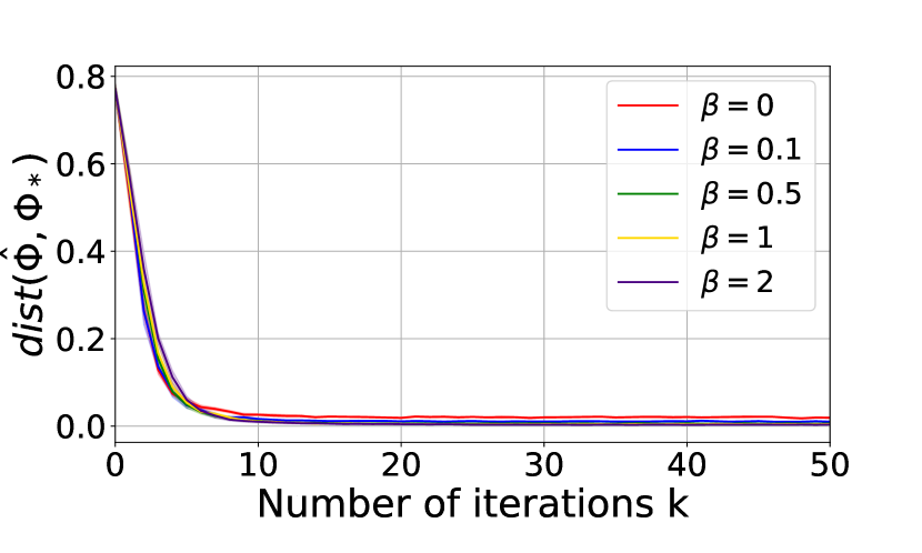
(a) DFW alt. minimization-descent (Algorithm 1)

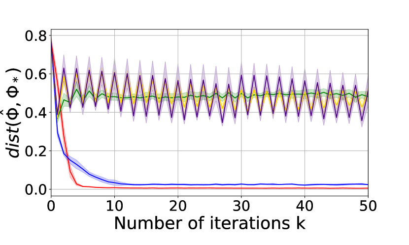
(b) Vanilla alt. minimization-descent (FedRep [1])

Figure 1: We compare subspace distance between the current and ground truth representation with respect to the number of iterations, where we vary non-isotropy through $\beta$. DFW suffers no degradation in performance when non-isotropy of the covariates increases, while FedRep fails catastrophically even under mild non-isotropy.

Figures (1(a)-1(b)) illustrate the influence of varying the degree of non-isotropy $\beta$: we examine its impact on the performance of DFW (Algorithm 1) and compare it with the vanilla alternating minimization-descent algorithm FedRep [1], which does not incorporate de-biasing and feature-whitening. The $\beta=0$ case corresponds to an identity covariance matrix, and our results show both algorithms are effective at recovering the representation as expected. Consistent with our theoretical guarantees, we find that DFW remains effective when the non-isotropy measure $\beta$ is increased; in contrast, Figure 1(b) shows how FedRep fails when dealing with even mildly non-isotropic data. This aligns with our findings in §3.1 and highlights the limitations of the vanilla representation gradient in handling non-isotropic feature data.

We now compare the benefit of multi-task setting over single-task. The problem dimensions $d_{x},d_{y},r,N$ are carried over from the previous experiment. We now introduce a different covariance matrix parameterization: $\Sigma_{x}=\frac{d_{x}\tilde{\Sigma}_{x}}{\text{Tr}(\tilde{\Sigma}_{x})}$, where $\tilde{\Sigma}_{x}=\frac{1}{2}(U+U^{\top})$, $U=5\cdot I_{d_{x}}+V$, with $V$ being a random matrix whose values are drawn from $\mathrm{Unif}(0,1)$. Figure 2(a) compares the performance of Algorithm 1 for the single-task ($H=1$) and multi-task settings ($H=25$), as well as FedRep ($H=25$). The figure highlights that DFW is able to make use of all source data to decrease variance and learn an accurate low-rank representation. As anticipated by our theoretical guarantees, Figure 2(a) demonstrates a significant reduction in the subspace distance as the number of tasks increases. Furthermore, the figure reveals that the vanilla alternating descent algorithm is not able to improve beyond a certain point, as predicted in §3.1.

4.2 System Identification

We consider a discrete-time linear system identification (sysID) problem, with dynamics

$$x[t+1]=Ax[t]+Bu[t]+w[t],\;\ t=0,\dots,T-1,$$

where $x[t]$ is the state of the system and $u[t]$ is the control input. In contrast to the previous example, the covariates are now additionally non-iid due to correlation over time. In particular, we can instantiate multi-task linear sysID in the form of (1),

$$x^{(h)}[t+1]=M^{(h)}_{\star}z^{(h)}[t]+w^{(h)}[t],\;\ t=0,\ldots,T-1$$

where $M^{(h)}_{\star}:=[A^{(h)}\;\ B^{(h)}]=F^{(h)}\Phi_{\star}\in\mathbb{R}^{d_{x}\times d_{z}}$. The state-action pair at time instant $t$ for all tasks $h\in[H]$ is embedded as $z^{(h)}[t]=[x^{(h)}[t]^{\top}\;\ u^{(h)}[t]^{\top}]^{\top}$. The process noise $w^{(i)}[t]$ and control action $u^{(h)}[t]$ are assumed to be drawn from Gaussian distributions $\mathcal{N}(0,\Sigma_{w})$ and $\mathcal{N}(0,\sigma^{2}_{u}I_{d_{u}})$, respectively, where $d_{u}$ represents the dimension of the control action. We set the state dimension $d_{x}=25$, control dimension $d_{u}=2$, latent dimension $r=6$, horizon $T=100$, and input variance $\sigma^{2}_{u}=1$. The generation process of the ground truth system matrices $M^{(h)}_{\star}$ follows a similar approach as described in the linear regression problem, with the addition of normalization step of the nominal weight matrix $F_{0}$ to ensure system stability for all tasks $h\in[H]$. Furthermore, the process noise covariance $\Sigma_{w}$ is parameterized in a similar manner as in the linear regression example, with $U=5\cdot I_{d_{x}}+2\cdot V$. The initial state $x^{(h)}[0]$ is drawn iid across tasks from the system’s stationary distribution $\mathcal{N}(0,\Sigma^{(h)}_{x})$, which is determined by the solution to the discrete Lyapunov equation $\Sigma^{(h)}_{x}=A^{(h)}\Sigma^{(h)}_{x}(A^{(h)})^{\top}+\sigma^{2}_{u}B^{(h)}(B^{(h)})^{\top}+\Sigma_{w}$. We note this implies the covariates $\mathopen{}x^{(h)}_{i}[t]\mathclose{}$ are inherently non-isotropic. Figure 2(b) again demonstrates the advantage of leveraging multi-task data to reduce the error in computing a shared representation across the system matrices $M^{(h)}_{\star}$. In line with our theoretical findings, DFW continues to benefit from multiple tasks, even when the data is non-iid. We see that FedRep remains suboptimal in this non-iid, non-isotropic setting.

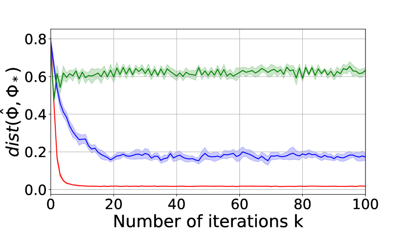
(a) IID linear regression with random covariance

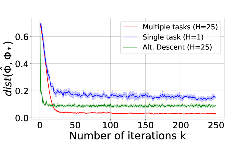
(b) Linear system identification

Figure 2: We plot the subspace distance between the current and ground truth representation with respect to the number of iterations, comparing between the single and multiple-task settings of Algorithm 1 and the multi-task FedRep. We observe performance improvement and variance reduction for multi-task DFW as predicted.

5 Discussion and Future Work

We propose an efficient algorithm to provably recover linear operators across multiple tasks to optimality from non-iid non-isotropic data, recovering near oracle empirical risk minimization rates. We show that the benefit of learning over multiple tasks manifests in a lower noise level in the optimization and smaller sample requirements for individual tasks. These results contribute toward a general understanding of representation learning from an algorithmic and statistical perspective. Some immediate open questions are: whether good initialization of the representation is necessary, and whether the convergence rate of DFW can be optimized e.g., through $\ell^{2}$-regularized weights $\mathopen{}\hat{F}^{(h)}\mathclose{}$. Resolving these questions has important implications for the natural extension of our framework: as emphasized in [1], the alternating empirical risk minimization (holding representation fixed) and gradient descent (holding task-specific weights fixed) framework naturally extends to the nonlinear setting. Providing guarantees for nonlinear function classes is an exciting and impactful avenue for future work, which concurrent work is moving toward, e.g. for $2$-layer ReLU networks [47] and kernel ridge regression [48]. It remains to be seen whether a computationally-efficient algorithm can be established for nonlinear meta-learning in the non-iid and non-isotropic data regime, while preserving joint scaling in number of tasks and data.

Appendix A Theoretical Analysis of DFW (Algorithm 1)

A.1 Preliminaries

We introduce some preliminary concepts and results that recur throughout our analysis. A fundamental concept in the analysis of least-squares solutions is the self-normalized martingale [40, 41].

Lemma 1 (cf. Zhang et al. [9, Lemma B.3])

Let $\{x_{t}\}_{t\geq 1}$ be a $\mathbb{R}^{d}$-valued process adapted to a filtration $\{\mathcal{F}_{t}\}_{t\geq 1}$. Let $\{\eta_{t}\}_{t\geq 1}$ be a $\mathbb{R}^{m}$-valued process adapted to $\{\mathcal{F}_{t}\}_{t\geq 2}$. Suppose that $\{\eta_{t}\}_{t\geq 1}$ is a $\sigma^{2}$-subgaussian martingale difference sequence, i.e.,:

$$\mathbb{E}[\eta_{t}\mid\mathcal{F}_{t}] =0,$$ (14)

$$\mathbb{E}[\exp(\lambda v^{\top}\eta_{t})\mid\mathcal{F}_{t}] \leq\exp\left(\frac{\lambda^{2}\sigma^{2}\left\|v\right\|^{2}}{2}\right)\>\>\forall\mathcal{F}_{t}\text{-measurable }\lambda\in\mathbb{R},v\in\mathbb{R}^{m}.$$ (15)

For $\Lambda\in\mathbb{R}^{m\times d}$, let $\{M_{t}(\Lambda)\}_{t\geq 1}$ be the $\mathbb{R}$-valued process:

$$M_{t}(\Lambda)=\exp\left(\frac{1}{\sigma}\sum_{i=1}^{t}\langle\Lambda x_{i},\eta_{i}\rangle-\frac{1}{2}\sum_{i=1}^{t}\left\|\Lambda x_{i}\right\|^{2}\right).$$ (16)

Then, the process $\{M_{t}(\Lambda)\}_{t\geq 1}$ satisfies $\mathbb{E}[M_{t}(\Lambda)]\leq 1$ for all $t\geq 1$.

In particular, this implies the following self-normalized martingale inequality that handles multiple matrix-valued self-normalized martingales. This can be seen as an instantiation of the Hilbert space variant from [41].

Proposition 1 (cf. Zhang et al. [9, Prop. B.1])

Fix $H\in\mathbb{N}_{+}$. For $h\in[H]$, let $\{x_{t}^{h},\eta_{t}^{h}\}_{t\geq 1}$ be a $\mathbb{R}^{d}\times\mathbb{R}^{m}$-valued process and $\{\mathcal{F}_{t}^{h}\}_{t\geq 1}$ be a filtration such that $\{x_{t}^{h}\}_{t\geq 1}$ is adapted to $\{\mathcal{F}_{t}^{h}\}_{t\geq 1}$, $\{\eta_{t}^{h}\}_{t\geq 1}$ is adapted to $\{\mathcal{F}_{t}^{h}\}_{t\geq 2}$, and $\{\eta_{t}^{h}\}_{t\geq 1}$ is a $\sigma^{2}$-subgaussian martingale difference sequence. Suppose that for all $h_{1}\neq h_{2}$, the process $\{x_{t}^{h_{1}},\eta_{t}^{h_{1}}\}$ is independent of $\{x_{t}^{h_{2}},\eta_{t}^{h_{2}}\}$. Fix (non-random) positive definite matrices $\{V^{h}\}_{h=1}^{H}$. For $t\geq 1$ and $h\in[H]$, define:

$$\bar{V}_{t}^{h}:=V^{h}+V^{h}_{t},\>\>V^{h}_{t}:=\sum_{i=1}^{t}x_{i}x_{i}^{\top},\>\>S_{t}^{h}:=\sum_{i=1}^{t}x_{i}\eta_{i}^{\top}.$$ (17)

For any fixed $T\in\mathbb{N}_{+}$, with probability at least $1-\delta$:

$$\sum_{h=1}^{H}\left\|(\bar{V}^{h}_{T})^{-1/2}S^{h}_{T}\right\|_{F}^{2}\leq 2\sigma^{2}\left[\sum_{h=1}^{H}\log\mathrm{det}((\bar{V}_{T}^{h})^{m/2}(V^{h})^{-m/2})+\log(1/\delta)\right].$$ (18)

We also consider the spectral norm variant of the self-normalized martingale bound.

Proposition 2 (Sarkar et al. [49, Proposition 8.2])

Let $\{x_{t}\}_{t\geq 1}$ be an $\mathbb{R}^{d}$-valued stochastic process adapted to filtration $\{\mathcal{F}_{t}\}_{t\geq 1}$ and $\{\eta_{t}\}_{t\geq 1}\subset\mathbb{R}^{m}$ be a $\sigma^{2}$-subgaussian martingale difference sequence adapted to $\{\mathcal{F}_{t}\}_{t\geq 2}$ as defined in Lemma 1. Fix a $\delta\in(0,1)$ and a non-random positive definite matrix $V\in\mathbb{R}^{d\times d}$. For $t\geq 1$, define $\bar{V}_{t}:=V+V_{t}$, $V_{t}:=\sum_{i=1}^{t}x_{i}x_{i}^{\top}$, $S_{t}:=\sum_{i=1}^{t}x_{i}\eta_{i}^{\top}$. Then with probability at least $1-\delta$,

$$\left\|(V_{T})^{-1/2}S_{T}\right\|^{2}\leq 8\sigma^{2}\left[\log\left(5^{m}\operatorname{\mathrm{det}}(\bar{V}_{T})^{1/2}\operatorname{\mathrm{det}}(V)^{-1/2}\right)+\log(1/\delta)\right].$$ (19)

We introduce the following useful two-sided concentration inequality for the sample covariance of iid subgaussian covariates.

Lemma 2 (Du et al. [3, Lemma A.6])

Let $x_{1},\dots,x_{T}\in\mathbb{R}^{d}$ be iid random vectors that satisfy $\mathbb{E}[x_{t}]=0$, $\mathbb{E}\left[x_{t}x_{t}^{\top}\right]=I_{d}$, and $x_{t}$ is $\gamma^{2}$-subgaussian. Fix $\delta\in(0,1)$. Suppose $T\gtrsim\gamma^{2}\left(d+\log(1/\delta)\right)$. Then with probability at least $1-\delta$, the following holds

$$0.9I_{d}\preceq\frac{1}{T}\sum_{i=1}^{T}x_{t}x_{t}^{\top}\preceq 1.1I_{d}.$$ (20)

In order to instantiate our bounds for non-iid covariates, we introduce the notions of $\beta$-mixing stationary processes [45, 50].

Definition 3 ($\beta$-mixing)

Let $\{x_{t}\}_{t\geq 1}$ be a $\mathbb{R}^{d}$-valued discrete-time stochastic process adapted to filtration $\{\mathcal{F}_{t}\}_{t=1}^{\infty}$. We denote the stationary distribution $\nu_{\infty}$. We define the $\beta$-mixing coefficient

$$\beta(k):=\sup_{t\geq 1}\mathbb{E}_{\left\{x_{\ell}\right\}_{\ell=1}^{t}}\left[\left\|\mathbb{P}_{x_{t+k}}(\cdot\mid\mathcal{F}_{t})-\nu_{\infty}\right\|_{\mathrm{tv}}\right],$$ (21)

where $\left\|\cdot\right\|_{\mathrm{tv}}$ denotes the total variation distance between probability measures.

Intuitively, the $\beta$-mixing coefficient measures how quickly on average a process mixes to the stationary distribution along any sample path. To see how $\beta$-mixing is instantiated, let $\left\{x_{t}\right\}_{t=1}^{T}$ be a sample path from a $\beta$-mixing process. Consider the following subsampled paths formed by taking every $a$-th covariate of $\left\{x_{t}\right\}$:

$$X^{T}_{(j)}:=\left\{x_{t}:1\leq t\leq T,\;(t-1\;\mathrm{mod}\;a)=j-1\right\},\;\;j=1,\dots,a.$$ (22)

Let the integers $m_{1},\dots,m_{a}$ and index sets $I_{(1)},\dots I_{(a)}$ denote the sizes and indices of $X^{T}_{(1)},\dots,X^{T}_{(a)}$, respectively. Finally, let $X^{m_{j}}_{\infty}$ denote a sequence of $m_{j}$ iid draws from the stationary distribution $\nu_{\infty}$. The following is a key lemma in relating a correlated process to iid draws.

Lemma 3 (Kuznetsov and Mohri [45, Proposition 2])

Let $g(\cdot)$ be a real-valued Borel-measurable function satisfying $-M_{1}\leq g(\cdot)\leq M_{2}$ for some $M_{1},M_{2}\geq 0$. Then, for all $j=1,\dots,a$.

$${\left|\mathbb{E}[g(X_{\infty}^{m_{j}})]-\mathbb{E}[g(X_{(j)}^{T})]\right|}\leq(M_{1}+M_{2})m_{j}\beta(a).$$

In our analysis, we often instantiate Lemma 3 with $g(\cdot)$ as an indicator function on a success event. For appropriately selected block length $a$, we are thus able to relate simpler iid analysis on $X_{\infty}^{m_{j}}$ to the original process $X^{T}_{(j)}$, accruing an additional factor in the failure probability. Lastly, we introduce a standard matrix concentration inequality.

Lemma 4 (Matrix Hoeffding [51])

Let $\{X_{h}\}_{h=1}^{H}\subset\mathbb{R}^{d\times d}$ be a sequence of independent, random symmetric matrices, and let $\{B_{h}\}_{h=1}^{H}$ be a sequence of fixed symmetric matrices. Assume each random matrix satisfies

$$\mathbb{E}\left[X_{h}\right]=0,\quad X_{h}^{2}\preceq B_{h}^{2}\text{ almost surely}.$$

Then for all $t\geq 0$,

$$\mathbb{P}\left[\lambda_{\max}\left(\sum_{h=1}^{H}X_{h}\right)\geq t\right]\leq d\cdot\exp\left(-\frac{t^{2}}{8\sigma^{2}}\right),\quad\sigma^{2}:=\left\|\sum_{h=1}^{H}B_{h}^{2}\right\|.$$

In particular, for general rectangular $\{M_{h}\}_{h=1}^{H}\subset\mathbb{R}^{d_{1}\times d_{2}}$, we may define $X_{h}:=\begin{bmatrix}0&M_{h}\\ M_{h}^{\top}&0\end{bmatrix}$ to yield a singular value concentration inequality. Assume each $M_{h}$ satisfies

$$\mathbb{E}\left[M_{h}\right]=0,\quad X_{h}^{2}\preceq B_{h}^{2}\text{ almost surely}.$$

Then for all $t\geq 0$,

$$\mathbb{P}\left[\sigma_{\max}\left(\sum_{h=1}^{H}M_{h}\right)\geq t\right]\leq(d_{1}+d_{2})\cdot\exp\left(-\frac{t^{2}}{8\sigma^{2}}\right),\quad\sigma^{2}:=\left\|\sum_{h=1}^{H}B_{h}^{2}\right\|.$$

As hinted by the indexing of the matrices, by leveraging the independence of processes across tasks $h$, Lemma 4 can be used to bound various quantities averaged across tasks, under the important caveat that the matrices are zero-mean, which ties back to the necessity of our de-biasing and feature-whitening adjustments.

A.2 The IID Setting

We recall that given the current representation iterate $\hat{\Phi}$, an iid draw of a multitask dataset $\{(\mathopen{}x^{(h)}_{i}[t]\mathclose{},\mathopen{}y^{(h)}_{i}[t]\mathclose{})\}_{t=1,i=1}^{T,N}$, $h=1,\dots,H$, and DFW trajectory partitions $\mathcal{N}_{1},\mathcal{N}_{2}$, the least squares weights $\mathopen{}\hat{F}^{(h)}\mathclose{}$ can be written as

$$\hat{F}^{(h)} =\operatorname*{argmin}_{F}\sum_{i\in\mathcal{N}_{1}}\sum_{t=1}^{T}\left\|\mathopen{}y^{(h)}_{i}[t]\mathclose{}-F\mathopen{}z^{(h)}_{i}[t]\mathclose{}\right\|^{2}$$

$$=F^{(h)}_{\star}\Phi_{\star}\mathopen{}X_{\mathcal{N}_{1}}^{(h)}\mathclose{}^{\top}\mathopen{}Z_{\mathcal{N}_{1}}^{(h)}\mathclose{}\left(\hat{\Sigma}^{(h)}_{z,\mathcal{N}_{1}T}\right)^{-1}+\mathopen{}W_{\mathcal{N}_{1}}^{(h)}\mathclose{}^{\top}\mathopen{}Z_{\mathcal{N}_{1}}^{(h)}\mathclose{}\left(\hat{\Sigma}^{(h)}_{z,\mathcal{N}_{1}T}\right)^{-1}$$

$$=\mathopen{}F^{(h)}_{\star}\mathclose{}\Phi_{\star}\hat{\Phi}^{\top}+\mathopen{}F^{(h)}_{\star}\mathclose{}\Phi_{\star}\left(I_{d_{x}}-\hat{\Phi}^{\top}\hat{\Phi}\right)\mathopen{}X_{\mathcal{N}_{1}}^{(h)}\mathclose{}^{\top}\mathopen{}Z_{\mathcal{N}_{1}}^{(h)}\mathclose{}\left(\hat{\Sigma}^{(h)}_{z,\mathcal{N}_{1}T}\right)^{-1}+\mathopen{}W_{\mathcal{N}_{1}}^{(h)}\mathclose{}^{\top}\mathopen{}Z_{\mathcal{N}_{1}}^{(h)}\mathclose{}\left(\hat{\Sigma}^{(h)}_{z,\mathcal{N}_{1}T}\right)^{-1}.$$ (23)

Now recalling the DFW representation update in the iid setting (6), we have

$$R\hat{\Phi}_{+} =\hat{\Phi}-\frac{\eta}{H}\sum_{h=1}^{H}\mathopen{}\hat{F}^{(h)}\mathclose{}^{\top}\left(\hat{F}^{(h)}\hat{\Phi}-F^{(h)}_{\star}\Phi_{\star}\right)-\frac{\eta}{H}\sum_{h=1}^{H}\mathopen{}\hat{F}^{(h)}\mathclose{}^{\top}\mathopen{}W_{\mathcal{N}_{2}}^{(h)}\mathclose{}^{\top}\mathopen{}X_{\mathcal{N}_{2}}^{(h)}\mathclose{}\left(\mathopen{}\hat{\Sigma}^{(h)}_{x,NT}\mathclose{}\right)^{-1}.$$ (24)

Right multiplying the update by $\Phi_{\star,\perp}^{\top}$, we get

$$R\hat{\Phi}_{+}\Phi_{\star,\perp}^{\top} =\hat{\Phi}\Phi_{\star,\perp}^{\top}-\frac{\eta}{H}\sum_{h=1}^{H}\mathopen{}\hat{F}^{(h)}\mathclose{}^{\top}\left(\hat{F}^{(h)}\hat{\Phi}-F^{(h)}_{\star}\Phi_{\star}\right)\Phi_{\star,\perp}^{\top}-\frac{\eta}{H}\sum_{h=1}^{H}\mathopen{}\hat{F}^{(h)}\mathclose{}^{\top}\mathopen{}W_{\mathcal{N}_{2}}^{(h)}\mathclose{}^{\top}\mathopen{}X_{\mathcal{N}_{2}}^{(h)}\mathclose{}\left(\hat{\Sigma}^{(h)}_{x,\mathcal{N}_{2}T}\right)^{-1}\Phi_{\star,\perp}^{\top}$$

$$=\left(I_{dx}-\frac{\eta}{H}\sum_{h=1}^{H}\mathopen{}\hat{F}^{(h)}\mathclose{}^{\top}\hat{F}^{(h)}\right)\hat{\Phi}\Phi_{\star,\perp}^{\top}-\frac{\eta}{H}\sum_{h=1}^{H}\mathopen{}\hat{F}^{(h)}\mathclose{}^{\top}\mathopen{}W_{\mathcal{N}_{2}}^{(h)}\mathclose{}^{\top}\mathopen{}X_{\mathcal{N}_{2}}^{(h)}\mathclose{}\left(\hat{\Sigma}^{(h)}_{x,\mathcal{N}_{2}T}\right)^{-1}\Phi_{\star,\perp}^{\top}$$

This naturally decomposes into a contraction term and a noise term. We start with an analysis of the noise term. We observe that since $\mathopen{}\hat{F}^{(h)}\mathclose{}$ is by construction independent of $\mathopen{}W_{\mathcal{N}_{2}}^{(h)}\mathclose{},\mathopen{}X_{\mathcal{N}_{2}}^{(h)}\mathclose{}$, by the independence of $\mathopen{}x^{(h)}_{i}[t]\mathclose{}$ across $t$ and $i$, and the noise independence $\mathopen{}w^{(h)}_{i}[t]\mathclose{}\perp\mathopen{}x^{(h)}_{i}[t]\mathclose{}$, we find

$$\mathbb{E}\left[\frac{1}{H}\sum_{h=1}^{H}\mathopen{}\hat{F}^{(h)}\mathclose{}^{\top}\mathopen{}W_{\mathcal{N}_{2}}^{(h)}\mathclose{}^{\top}\mathopen{}X_{\mathcal{N}_{2}}^{(h)}\mathclose{}\left(\hat{\Sigma}^{(h)}_{x,\mathcal{N}_{2}T}\right)^{-1}\right] =\frac{1}{H}\sum_{h=1}^{H}\mathbb{E}\left[\mathopen{}\hat{F}^{(h)}\mathclose{}\right]^{\top}\mathbb{E}\left[\mathopen{}W_{\mathcal{N}_{2}}^{(h)}\mathclose{}\right]\mathbb{E}\left[\mathopen{}X_{\mathcal{N}_{2}}^{(h)}\mathclose{}\left(\hat{\Sigma}^{(h)}_{x,\mathcal{N}_{2}T}\right)^{-1}\right]=0.$$

Therefore, we set up for an application of Lemma 4. Toward doing so, we prove the following two ingredients: 1. a high probability bound on $\left\|\mathopen{}\hat{F}^{(h)}\mathclose{}\right\|$, 2. a high probability bound on the least-squares noise-esque term $\left\|\mathopen{}\hat{F}^{(h)}\mathclose{}^{\top}\mathopen{}W_{\mathcal{N}_{2}}^{(h)}\mathclose{}^{\top}\mathopen{}X_{\mathcal{N}_{2}}^{(h)}\mathclose{}\left(\hat{\Sigma}^{(h)}_{x,\mathcal{N}_{2}T}\right)^{-1}\right\|$. We then condition on these two high-probability events to instantiate the almost-sure boundedness in Lemma 4. We start with the analysis of $\mathopen{}\hat{F}^{(h)}\mathclose{}$. We observe trivially that

$$\left\|\mathopen{}\hat{F}^{(h)}\mathclose{}\right\| \leq\left\|\mathopen{}F^{(h)}_{\star}\mathclose{}\right\|+\left\|\mathopen{}F^{(h)}_{\star}\mathclose{}\right\|\left\|\Phi_{\star}\mathcal{P}_{\hat{\Phi}}^{\perp}\right\|\left\|\mathopen{}X_{\mathcal{N}_{1}}^{(h)}\mathclose{}^{\top}\mathopen{}Z_{\mathcal{N}_{1}}^{(h)}\mathclose{}\left(\hat{\Sigma}^{(h)}_{z,\mathcal{N}_{1}T}\right)^{-1}\right\|+\left\|\mathopen{}W_{\mathcal{N}_{1}}^{(h)}\mathclose{}^{\top}\mathopen{}Z_{\mathcal{N}_{1}}^{(h)}\mathclose{}\left(\hat{\Sigma}^{(h)}_{z,\mathcal{N}_{1}T}\right)^{-1}\right\|.$$

Lemma 5

Let ${\left|\mathcal{N}_{1}\right|}T\gtrsim\gamma^{2}\left(\max\left\{d_{y},r\right\}+\log(1/\delta)\right)$. Then, with probability greater than $1-\delta$, we have

$$\left\|\mathopen{}X_{\mathcal{N}_{1}}^{(h)}\mathclose{}^{\top}\mathopen{}Z_{\mathcal{N}_{1}}^{(h)}\mathclose{}\left(\hat{\Sigma}^{(h)}_{z,\mathcal{N}_{1}T}\right)^{-1}\right\| \leq\frac{2}{3}\left(\kappa\left(\mathopen{}\Sigma^{(h)}_{x}\mathclose{}\right)+1\right),$$ (25)

$$\left\|\mathopen{}W_{\mathcal{N}_{1}}^{(h)}\mathclose{}^{\top}\mathopen{}Z_{\mathcal{N}_{1}}^{(h)}\mathclose{}\left(\hat{\Sigma}^{(h)}_{z,\mathcal{N}_{1}T}\right)^{-1}\right\| \leq 6\mathopen{}\sigma^{(h)}_{w}\mathclose{}\sqrt{\frac{d_{y}+\log(1/\delta)}{\lambda_{\min}(\mathopen{}\Sigma^{(h)}_{x}\mathclose{}){\left|\mathcal{N}_{1}\right|}T}}.$$ (26)

Therefore, setting ${\left|\mathcal{N}_{1}\right|}T\gtrsim\max\left\{\gamma^{2},\frac{\mathopen{}\sigma^{(h)}_{w}\mathclose{}^{2}}{\lambda_{\min}(\mathopen{}\Sigma^{(h)}_{x}\mathclose{})}\right\}\left(d_{y}+\log(1/\delta)\right)$, under the assumption that $\left\|\Phi_{\star}\mathcal{P}_{\hat{\Phi}}^{\perp}\right\|\leq\frac{3}{\kappa\left(\mathopen{}\Sigma^{(h)}_{x}\mathclose{}\right)+1}$, we get a high-probability bound on $\mathopen{}\hat{F}^{(h)}\mathclose{}$.

Lemma 6

Assume ${\left|\mathcal{N}_{1}\right|}T\gtrsim\max\left\{\gamma^{2},\frac{\mathopen{}\sigma^{(h)}_{w}\mathclose{}^{2}}{\lambda_{\min}(\mathopen{}\Sigma^{(h)}_{x}\mathclose{})}\right\}\left(\max\left\{d_{y},r\right\}+\log(1/\delta)\right)$ and $\left\|\Phi_{\star}\mathcal{P}_{\hat{\Phi}}^{\perp}\right\|\leq\frac{3}{\kappa\left(\mathopen{}\Sigma^{(h)}_{x}\mathclose{}\right)+1}$. Then with probability at least $1-\delta$

$$\left\|\mathopen{}\hat{F}^{(h)}\mathclose{}\right\| \leq 2\left\|\mathopen{}F^{(h)}_{\star}\mathclose{}\right\|.$$ (27)

Denote the event on which Lemma 6 holds with probability at least $1-\delta$ as $\mathcal{E}_{\mathopen{}\hat{F}^{(h)}\mathclose{}}(\delta)$. Then, conditioned on $\mathcal{E}_{\mathopen{}\hat{F}^{(h)}\mathclose{}}(\delta)$, we observe that $\mathopen{}\hat{F}^{(h)}\mathclose{}\mathopen{}W_{\mathcal{N}_{2}}^{(h)}\mathclose{}$ is a $4\mathopen{}\sigma^{(h)}_{w}\mathclose{}^{2}\|\mathopen{}F^{(h)}_{\star}\mathclose{}\|^{2}$-subgaussian MDS supported on $\mathbb{R}^{r}$. Therefore, bounding

$$\left\|\mathopen{}\hat{F}^{(h)}\mathclose{}^{\top}\mathopen{}W_{\mathcal{N}_{2}}^{(h)}\mathclose{}^{\top}\mathopen{}X_{\mathcal{N}_{2}}^{(h)}\mathclose{}\left(\hat{\Sigma}^{(h)}_{x,\mathcal{N}_{2}T}\right)^{-1}\right\|\leq\left\|\mathopen{}\hat{F}^{(h)}\mathclose{}\mathopen{}W_{\mathcal{N}_{2}}^{(h)}\mathclose{}^{\top}\mathopen{}X_{\mathcal{N}_{2}}^{(h)}\mathclose{}\left(\hat{\Sigma}^{(h)}_{x,\mathcal{N}_{2}T}\right)^{-1/2}\right\|\lambda_{\min}(\hat{\Sigma}^{(h)}_{x,\mathcal{N}_{2}T})^{-1/2},$$

we invoke Proposition 2 and Lemma 2, we get the following bound

Lemma 7

Let the conditions of Lemma 6 hold. Then, conditioned on the success event $\mathcal{E}_{\mathopen{}\hat{F}^{(h)}\mathclose{}}(\delta)$, with probability at least $1-\delta$,

$$\left\|\mathopen{}\hat{F}^{(h)}\mathclose{}^{\top}\mathopen{}W_{\mathcal{N}_{2}}^{(h)}\mathclose{}^{\top}\mathopen{}X_{\mathcal{N}_{2}}^{(h)}\mathclose{}\left(\hat{\Sigma}^{(h)}_{x,\mathcal{N}_{2}T}\right)^{-1}\right\| \leq 12\mathopen{}\sigma^{(h)}_{w}\mathclose{}\|F^{(h)}_{\star}\|\sqrt{\frac{d_{x}+\log(1/\delta)}{\lambda_{\min}(\mathopen{}\Sigma^{(h)}_{x}\mathclose{}){\left|\mathcal{N}_{2}\right|}T}}.$$ (28)

Therefore, we have provided a high-probability bound on the task-wise noise term. Define the matrices

$$B^{(h)} :=12\frac{\mathopen{}\sigma^{(h)}_{w}\mathclose{}\|F^{(h)}_{\star}\|}{H}\sqrt{\frac{d_{x}+\log(H/\delta)}{\lambda_{\min}(\mathopen{}\Sigma^{(h)}_{x}\mathclose{}){\left|\mathcal{N}_{2}\right|}T}}\cdot I_{d_{y}+r}.$$

Union-bounding over the high probability bound events of Lemma 7 with probability $1-\delta/H$ each and setting $B^{(h)}$ as above, we may apply Lemma 4 with $\sigma^{2}:=\sum_{h}{B^{(h)}}^{2}$ to yield the following bound.

Lemma 8

Conditioning on the bounds of Lemma 7 holding with probability at least $1-\delta/H$ for each $h\in[H]$, we have with probability at least $1-\delta$,

$$\left\|\frac{\eta}{H}\sum_{h=1}^{H}\mathopen{}\hat{F}^{(h)}\mathclose{}^{\top}\mathopen{}W_{\mathcal{N}_{2}}^{(h)}\mathclose{}^{\top}\mathopen{}X_{\mathcal{N}_{2}}^{(h)}\mathclose{}\left(\hat{\Sigma}^{(h)}_{x,\mathcal{N}_{2}T}\right)^{-1}\right\| \lesssim\max_{h}\;\frac{\eta\mathopen{}\sigma^{(h)}_{w}\mathclose{}\|F^{(h)}_{\star}\|}{\sqrt{H{\left|\mathcal{N}_{2}\right|}T}}\sqrt{\frac{d_{x}+\log(H/\delta)}{\lambda_{\min}(\mathopen{}\Sigma^{(h)}_{x}\mathclose{})}\log\left(\frac{d_{y}+r}{\delta}\right)}.$$

Importantly, setting ${\left|\mathcal{N}_{2}\right|}=\Theta(N)$, we note that this establishes the desired $\tilde{O}\left(1/\sqrt{HNT}\right)$ scaling of the noise term. We note that our application of Matrix Hoeffding is rather crude, and the above bound can likely be improved in terms of polylog$(1/\delta)$ factors.

We now move on to bounding the contraction term. Defining

$$\mathopen{}\Delta^{(h)}\mathclose{} :=\mathopen{}F^{(h)}_{\star}\mathclose{}\Phi_{\star}\left(I_{d_{x}}-\hat{\Phi}^{\top}\hat{\Phi}\right)\mathopen{}X_{\mathcal{N}_{1}}^{(h)}\mathclose{}^{\top}\mathopen{}Z_{\mathcal{N}_{1}}^{(h)}\mathclose{}\left(\hat{\Sigma}^{(h)}_{z,\mathcal{N}_{1}T}\right)^{-1}$$

$$\mathopen{}E^{(h)}\mathclose{} :=\mathopen{}W_{\mathcal{N}_{1}}^{(h)}\mathclose{}^{\top}\mathopen{}Z_{\mathcal{N}_{1}}^{(h)}\mathclose{}\left(\hat{\Sigma}^{(h)}_{z,\mathcal{N}_{1}T}\right)^{-1},$$

we write (23) as $\mathopen{}\hat{F}^{(h)}\mathclose{}=\mathopen{}F^{(h)}_{\star}\mathclose{}\Phi_{\star}\hat{\Phi}^{\top}+\mathopen{}\Delta^{(h)}\mathclose{}+\mathopen{}E^{(h)}\mathclose{}$. Expanding

$$\mathopen{}\hat{F}^{(h)}\mathclose{}^{\top}\mathopen{}\hat{F}^{(h)}\mathclose{} =\hat{\Phi}\Phi_{\star}^{\top}\mathopen{}F^{(h)}_{\star}\mathclose{}^{\top}\mathopen{}F^{(h)}_{\star}\mathclose{}\Phi_{\star}\hat{\Phi}^{\top}+\mathopen{}\Delta^{(h)}\mathclose{}^{\top}\mathopen{}\Delta^{(h)}\mathclose{}+\mathopen{}E^{(h)}\mathclose{}^{\top}\mathopen{}E^{(h)}\mathclose{}$$

$$\quad+\mathrm{Sym}(\mathopen{}\Delta^{(h)}\mathclose{}^{\top}\mathopen{}F^{(h)}_{\star}\mathclose{}\Phi_{\star}\hat{\Phi}^{\top})+\mathrm{Sym}(\mathopen{}E^{(h)}\mathclose{}^{\top}\mathopen{}F^{(h)}_{\star}\mathclose{}\Phi_{\star}\hat{\Phi}^{\top})+\mathrm{Sym}(\mathopen{}\Delta^{(h)}\mathclose{}^{\top}\mathopen{}E^{(h)}\mathclose{}),$$

where $\mathrm{Sym}(A):=A+A^{\top}$. From Lemma 6, we immediately get an upper bound on $\lambda_{\max}(\mathopen{}\hat{F}^{(h)}\mathclose{}^{\top}\mathopen{}\hat{F}^{(h)}\mathclose{})\leq 4\left\|\mathopen{}F^{(h)}_{\star}\mathclose{}\right\|^{2}$. To lower bound $\lambda_{\min}(\mathopen{}\hat{F}^{(h)}\mathclose{}^{\top}\mathopen{}\hat{F}^{(h)}\mathclose{})$, we observe that the diagonal terms $\mathopen{}\Delta^{(h)}\mathclose{}^{\top}\mathopen{}\Delta^{(h)}\mathclose{}$, $\mathopen{}E^{(h)}\mathclose{}^{\top}\mathopen{}E^{(h)}\mathclose{}$ are pd, and thus can be ignored. We then observe that by Weyl’s inequality [52], we have

$$\lambda_{\min}(\mathopen{}\hat{F}^{(h)}\mathclose{}^{\top}\mathopen{}\hat{F}^{(h)}\mathclose{}) \geq\lambda_{\min}\left(\hat{\Phi}\Phi_{\star}^{\top}\mathopen{}F^{(h)}_{\star}\mathclose{}^{\top}\mathopen{}F^{(h)}_{\star}\mathclose{}\Phi_{\star}\hat{\Phi}^{\top}\right)$$

$$\quad-\lambda_{\max}\left(\mathrm{Sym}(\mathopen{}\Delta^{(h)}\mathclose{}^{\top}\mathopen{}F^{(h)}_{\star}\mathclose{}\Phi_{\star}\hat{\Phi}^{\top})+\mathrm{Sym}(\mathopen{}E^{(h)}\mathclose{}^{\top}\mathopen{}F^{(h)}_{\star}\mathclose{}\Phi_{\star}\hat{\Phi}^{\top})+\mathrm{Sym}(\mathopen{}\Delta^{(h)}\mathclose{}^{\top}\mathopen{}E^{(h)}\mathclose{})\right).$$

We further observe that

$$\lambda_{\max}(\mathrm{Sym}(A)) =\max_{\left\|x\right\|=1}x^{\top}(A+A^{\top})x$$

$$\leq\max_{\left\|u\right\|,\left\|v\right\|=1}x^{\top}Av+x^{\top}A^{\top}v$$

$$\leq 2\left\|A\right\|,$$

such that the cross terms may be bounded as

$$\lambda_{\max}\left(\mathrm{Sym}(\mathopen{}\Delta^{(h)}\mathclose{}^{\top}\mathopen{}F^{(h)}_{\star}\mathclose{}\Phi_{\star}\hat{\Phi}^{\top})+\mathrm{Sym}(\mathopen{}E^{(h)}\mathclose{}^{\top}\mathopen{}F^{(h)}_{\star}\mathclose{}\Phi_{\star}\hat{\Phi}^{\top})+\mathrm{Sym}(\mathopen{}\Delta^{(h)}\mathclose{}^{\top}\mathopen{}E^{(h)}\mathclose{})\right)$$

$$\leq\; 2\left\|\mathopen{}\Delta^{(h)}\mathclose{}^{\top}\mathopen{}F^{(h)}_{\star}\mathclose{}\Phi_{\star}\hat{\Phi}^{\top}\right\|+2\left\|\mathopen{}E^{(h)}\mathclose{}^{\top}\mathopen{}F^{(h)}_{\star}\mathclose{}\Phi_{\star}\hat{\Phi}^{\top}\right\|+2\left\|\mathopen{}\Delta^{(h)}\mathclose{}^{\top}\mathopen{}E^{(h)}\mathclose{}\right\|$$

$$=\; 2\left\|\mathopen{}\Delta^{(h)}\mathclose{}\right\|\left\|\mathopen{}F^{(h)}_{\star}\mathclose{}\right\|+2\left\|\mathopen{}E^{(h)}\mathclose{}\right\|\left\|\mathopen{}F^{(h)}_{\star}\mathclose{}\right\|+2\left\|\mathopen{}\Delta^{(h)}\mathclose{}\right\|\left\|\mathopen{}E^{(h)}\mathclose{}\right\|.$$

Applying a similar analysis as in Lemma 5, we derive the following.

Lemma 9

Assume ${\left|\mathcal{N}_{1}\right|}T\gtrsim\max\left\{\gamma^{2},\frac{\mathopen{}\sigma^{(h)}_{w}\mathclose{}^{2}}{\lambda_{\min}(\mathopen{}\Sigma^{(h)}_{x}\mathclose{})}\frac{\left\|F_{\star}\right\|^{2}}{\sigma_{\min}(F^{(h)}_{\star})^{4}}\right\}\left(\max\left\{d_{y},r\right\}+\log(1/\delta)\right)$, and $\left\|\Phi_{\star}\mathcal{P}_{\hat{\Phi}}^{\perp}\right\|\leq\frac{3}{2}\frac{c}{\kappa\left(\mathopen{}\Sigma^{(h)}_{x}\mathclose{}\right)+1}\frac{\sigma_{\min}(F^{(h)}_{\star})^{2}}{\left\|F_{\star}\right\|}$, where $c>0$ is a sufficiently small, fixed numerical constant. Then with probability at least $1-\delta$,

$$\lambda_{\max}\left(\mathrm{Sym}(\mathopen{}\Delta^{(h)}\mathclose{}^{\top}\mathopen{}F^{(h)}_{\star}\mathclose{}\Phi_{\star}\hat{\Phi}^{\top})+\mathrm{Sym}(\mathopen{}E^{(h)}\mathclose{}^{\top}\mathopen{}F^{(h)}_{\star}\mathclose{}\Phi_{\star}\hat{\Phi}^{\top})+\mathrm{Sym}(\mathopen{}\Delta^{(h)}\mathclose{}^{\top}\mathopen{}E^{(h)}\mathclose{})\right)\leq 3c\sigma_{\min}(\mathopen{}F^{(h)}_{\star}\mathclose{})^{2}.$$

Now, using the fact that

$$\lambda_{\min}\left(\hat{\Phi}\Phi_{\star}^{\top}\mathopen{}F^{(h)}_{\star}\mathclose{}^{\top}\mathopen{}F^{(h)}_{\star}\mathclose{}\Phi_{\star}\hat{\Phi}^{\top}\right) =\min_{\left\|x\right\|=1}x^{\top}\hat{\Phi}\Phi_{\star}^{\top}\mathopen{}F^{(h)}_{\star}\mathclose{}^{\top}\mathopen{}F^{(h)}_{\star}\mathclose{}\Phi_{\star}\hat{\Phi}^{\top}x$$

$$\geq\lambda_{\min}\left(\mathopen{}F^{(h)}_{\star}\mathclose{}^{\top}\mathopen{}F^{(h)}_{\star}\mathclose{}\right)\min_{\left\|x\right\|=1}x^{\top}\hat{\Phi}\Phi_{\star}^{\top}\Phi_{\star}\hat{\Phi}^{\top}x$$

$$=\lambda_{\min}\left(\mathopen{}F^{(h)}_{\star}\mathclose{}^{\top}\mathopen{}F^{(h)}_{\star}\mathclose{}\right)\sigma_{\min}^{2}\left(\Phi_{\star}\hat{\Phi}^{\top}\right).$$

To further lower bound $\sigma_{\min}^{2}\left(\Phi_{\star}\hat{\Phi}^{\top}\right)$, we observe that

$$\hat{\Phi}\hat{\Phi}^{\top} =\hat{\Phi}\left(\Phi_{\star}^{\top}\Phi_{\star}+\Phi_{\star,\perp}^{\top}\Phi_{\star,\perp}\right)\hat{\Phi}^{\top}$$

$$\implies 1=\lambda_{\max}(\hat{\Phi}\hat{\Phi}^{\top}) \leq\lambda_{\min}\left(\hat{\Phi}\Phi_{\star}^{\top}\Phi_{\star}\hat{\Phi}^{\top}\right)+\lambda_{\max}\left(\hat{\Phi}\Phi_{\star,\perp}^{\top}\Phi_{\star,\perp}\hat{\Phi}^{\top}\right)\quad\text{Weyl's inequality}$$

$$\implies\sigma_{\min}^{2}\left(\Phi_{\star}\hat{\Phi}^{\top}\right) \geq 1-\left\|\Phi_{\star,\perp}\hat{\Phi}^{\top}\right\|^{2}.$$

Under the assumption that $\left\|\Phi_{\star,\perp}\hat{\Phi}^{\top}\right\|=\left\|\Phi_{\star}\mathcal{P}_{\hat{\Phi}}^{\perp}\right\|$ is sufficiently small, e.g., $\left\|\Phi_{\star,\perp}\hat{\Phi}^{\top}\right\|\leq 1/2$ such that $1-\left\|\Phi_{\star,\perp}\hat{\Phi}^{\top}\right\|^{2}\geq 3/4$, then we have the following lower bound on $\lambda_{\min}(\mathopen{}\hat{F}^{(h)}\mathclose{}^{\top}\mathopen{}\hat{F}^{(h)}\mathclose{})$: with probability at least $1-\delta$

$$\lambda_{\min}(\mathopen{}\hat{F}^{(h)}\mathclose{}^{\top}\mathopen{}\hat{F}^{(h)}\mathclose{}) \geq\left(\frac{3}{4}-3c\right)\lambda_{\min}(\mathopen{}F^{(h)}_{\star}\mathclose{}^{\top}\mathopen{}F^{(h)}_{\star}\mathclose{}).$$

As such, for $\eta\leq\min_{h}\frac{1}{4\|\mathopen{}F^{(h)}_{\star}\mathclose{}\|^{2}}$ we may bound the contraction factor by

$$\left\|I_{d_{x}}-\eta\frac{1}{H}\sum_{h=1}^{H}\mathopen{}\hat{F}^{(h)}\mathclose{}^{\top}\mathopen{}\hat{F}^{(h)}\mathclose{}\right\| \leq\left(1-\eta\left(\frac{3}{4}-3c\right)\frac{1}{H}\sum_{h=1}^{H}\sigma_{\min}(\mathopen{}F^{(h)}_{\star}\mathclose{})^{2}\right).$$

Piecing this together, we have the following

Lemma 10

Assume ${\left|\mathcal{N}_{1}\right|}T\gtrsim\max\left\{\gamma^{2},\frac{\mathopen{}\sigma^{(h)}_{w}\mathclose{}^{2}}{\lambda_{\min}(\mathopen{}\Sigma^{(h)}_{x}\mathclose{})}\frac{\left\|F_{\star}\right\|^{2}}{\sigma_{\min}(F^{(h)}_{\star})^{4}}\right\}\left(\max\left\{d_{y},r\right\}+\log(H/\delta)\right)$, and $\left\|\Phi_{\star}\mathcal{P}_{\hat{\Phi}}^{\perp}\right\|\leq\min\left\{\frac{3}{16}\frac{1}{\kappa\left(\mathopen{}\Sigma^{(h)}_{x}\mathclose{}\right)+1}\frac{\sigma_{\min}(F^{(h)}_{\star})^{2}}{\left\|F_{\star}\right\|},1/2\right\}$. Let $\eta\leq\min_{h}1/4\|\mathopen{}F^{(h)}_{\star}\mathclose{}\|^{2}$. There exists numerical constant $C>0$ such that the following holds: with probability at least $1-\delta$,

$$\left\|R\hat{\Phi}_{+}\Phi_{\star,\perp}^{\top}\right\| \leq\left(1-\frac{3\eta}{8}\frac{1}{H}\sum_{h=1}^{H}\sigma_{\min}(\mathopen{}F^{(h)}_{\star}\mathclose{})^{2}\right)\left\|\hat{\Phi}\Phi_{\star,\perp}^{\top}\right\|+\max_{h}\;C\frac{\eta\mathopen{}\sigma^{(h)}_{w}\mathclose{}\|F^{(h)}_{\star}\|}{\sqrt{H{\left|\mathcal{N}_{2}\right|}T}}\sqrt{\frac{d_{x}+\log(H/\delta)}{\lambda_{\min}(\mathopen{}\Sigma^{(h)}_{x}\mathclose{})}\log\left(\frac{d_{y}+r}{\delta}\right)},$$

The last remaining step is to bound the effect of the orthogonalization factor $R$. We want to upper bound $\|R^{-1}\|=1/\sigma_{\min}(R)$, and thus it suffices to lower bound $\sigma_{\min}(R)$. By definition, we have

$$RR^{\top}=(R\hat{\Phi}_{+})(R\hat{\Phi}_{+})^{\top}$$

$$=\; \left(\hat{\Phi}-\frac{\eta}{H}\sum_{h=1}^{H}\mathopen{}\hat{F}^{(h)}\mathclose{}^{\top}\left(\hat{F}^{(h)}\hat{\Phi}-F^{(h)}_{\star}\Phi_{\star}\right)-\frac{\eta}{H}\sum_{h=1}^{H}\mathopen{}\hat{F}^{(h)}\mathclose{}^{\top}\mathopen{}W^{(h)}\mathclose{}^{\top}\mathopen{}X^{(h)}\mathclose{}\left(\mathopen{}\hat{\Sigma}^{(h)}_{x,NT}\mathclose{}\right)^{-1}\right)$$

$$\left(\hat{\Phi}-\frac{\eta}{H}\sum_{h=1}^{H}\mathopen{}\hat{F}^{(h)}\mathclose{}^{\top}\left(\hat{F}^{(h)}\hat{\Phi}-F^{(h)}_{\star}\Phi_{\star}\right)-\frac{\eta}{H}\sum_{h=1}^{H}\mathopen{}\hat{F}^{(h)}\mathclose{}^{\top}\mathopen{}W^{(h)}\mathclose{}^{\top}\mathopen{}X^{(h)}\mathclose{}\left(\mathopen{}\hat{\Sigma}^{(h)}_{x,NT}\mathclose{}\right)^{-1}\right)^{\top}$$

$$\succeq\; I_{r}-\mathrm{Sym}\left(\frac{\eta}{H}\sum_{h=1}^{H}\mathopen{}\hat{F}^{(h)}\mathclose{}^{\top}\left(\hat{F}^{(h)}\hat{\Phi}-F^{(h)}_{\star}\Phi_{\star}\right)\hat{\Phi}^{\top}\right)-\mathrm{Sym}\left(\frac{\eta}{H}\sum_{h=1}^{H}\mathopen{}\hat{F}^{(h)}\mathclose{}^{\top}\mathopen{}W^{(h)}\mathclose{}^{\top}\mathopen{}X^{(h)}\mathclose{}\left(\mathopen{}\hat{\Sigma}^{(h)}_{x,NT}\mathclose{}\right)^{-1}\hat{\Phi}^{\top}\right)$$

$$\quad+\mathrm{Sym}\left(\frac{\eta^{2}}{H^{2}}\mathopen{}\hat{F}^{(h)}\mathclose{}^{\top}\left(\hat{F}^{(h)}\hat{\Phi}-F^{(h)}_{\star}\Phi_{\star}\right)^{\top}\left(\sum_{h=1}^{H}\mathopen{}\hat{F}^{(h)}\mathclose{}^{\top}\mathopen{}W^{(h)}\mathclose{}^{\top}\mathopen{}X^{(h)}\mathclose{}\left(\mathopen{}\hat{\Sigma}^{(h)}_{x,NT}\mathclose{}\right)^{-1}\right)^{\top}\right),$$

where we discarded the pd diagonal terms of the expansion. Focusing on the first cross term, we have

$$\mathrm{Sym}\left(\frac{\eta}{H}\sum_{h=1}^{H}\mathopen{}\hat{F}^{(h)}\mathclose{}^{\top}\left(\hat{F}^{(h)}\hat{\Phi}-F^{(h)}_{\star}\Phi_{\star}\right)\hat{\Phi}^{\top}\right)$$

$$=\; \frac{\eta}{H}\sum_{h=1}^{H}\mathrm{Sym}\left(\mathopen{}\hat{F}^{(h)}\mathclose{}^{\top}\mathopen{}\hat{F}^{(h)}\mathclose{}-\mathopen{}\hat{F}^{(h)}\mathclose{}^{\top}\mathopen{}F^{(h)}_{\star}\mathclose{}\Phi_{\star}\hat{\Phi}^{\top}\right)$$

$$=\; \frac{\eta}{H}\sum_{h}\mathrm{Sym}\left(\mathopen{}\hat{F}^{(h)}\mathclose{}^{\top}\left(\mathopen{}F^{(h)}_{\star}\mathclose{}\Phi_{\star}\left(I_{d_{x}}-\hat{\Phi}^{\top}\hat{\Phi}\right)\mathopen{}X_{\mathcal{N}_{1}}^{(h)}\mathclose{}^{\top}\mathopen{}Z_{\mathcal{N}_{1}}^{(h)}\mathclose{}\left(\hat{\Sigma}^{(h)}_{z,\mathcal{N}_{1}T}\right)^{-1}+\mathopen{}W_{\mathcal{N}_{1}}^{(h)}\mathclose{}^{\top}\mathopen{}Z_{\mathcal{N}_{1}}^{(h)}\mathclose{}\left(\hat{\Sigma}^{(h)}_{z,\mathcal{N}_{1}T}\right)^{-1}\right)\right).$$

Conditioning on the high probability bound events of Lemma 5 and Lemma 6, we repeat a similar analysis as Lemma 9 to yield

$$\sigma_{\min}(R)^{2}\geq 1-\frac{4c\eta}{H}\sum_{h}\left\|\mathopen{}F^{(h)}_{\star}\mathclose{}\right\|^{2}.$$

Therefore, for appropriately chosen numerical constant $c>0$, we have

$$\sigma_{\min}(R)\left\|I_{d_{x}}-\frac{\eta}{H}\sum_{h=1}^{H}\mathopen{}\hat{F}^{(h)}\mathclose{}^{\top}\mathopen{}\hat{F}^{(h)}\mathclose{}\right\|\leq\left(1-\frac{3\eta}{16}\frac{1}{H}\sum_{h=1}^{H}\sigma_{\min}(\mathopen{}F^{(h)}_{\star}\mathclose{})^{2}\right)^{1/2}.$$

Combining the above lemmas culminates in the final descent guarantee.

Theorem 3 (Full version of Theorem 2)

Assume ${\left|\mathcal{N}_{1}\right|}T\gtrsim\max\left\{\gamma^{2},\frac{\mathopen{}\sigma^{(h)}_{w}\mathclose{}^{2}}{\lambda_{\min}(\mathopen{}\Sigma^{(h)}_{x}\mathclose{})}\frac{\left\|F_{\star}\right\|^{2}}{\sigma_{\min}(F^{(h)}_{\star})^{4}}\right\}\left(\max\left\{d_{y},r\right\}+\log(H/\delta)\right)$, and $\left\|\hat{\Phi}\Phi_{\star,\perp}^{\top}\right\|\leq\min\left\{\frac{3}{16}\frac{1}{\kappa\left(\mathopen{}\Sigma^{(h)}_{x}\mathclose{}\right)+1}\frac{\sigma_{\min}(F^{(h)}_{\star})^{2}}{\left\|F_{\star}\right\|},1/2\right\}$. Let $\eta\leq\min_{h}1/4\|\mathopen{}F^{(h)}_{\star}\mathclose{}\|^{2}$. There exists numerical constant $C>0$ such that the following holds: with probability at least $1-\delta$,

$$\left\|\hat{\Phi}_{+}\Phi_{\star,\perp}^{\top}\right\| \leq\left(1-\frac{3\eta}{16}\frac{1}{H}\sum_{h=1}^{H}\sigma_{\min}(\mathopen{}F^{(h)}_{\star}\mathclose{})^{2}\right)^{1/2}\left\|\hat{\Phi}\Phi_{\star,\perp}^{\top}\right\|$$

$$\quad+\max_{h}\;C\frac{\eta\mathopen{}\sigma^{(h)}_{w}\mathclose{}\|F^{(h)}_{\star}\|}{\sqrt{H{\left|\mathcal{N}_{2}\right|}T}}\sqrt{\frac{d_{x}+\log(H/\delta)}{\lambda_{\min}(\mathopen{}\Sigma^{(h)}_{x}\mathclose{})}\log\left(\frac{d_{y}+r}{\delta}\right)}.$$

A.3 The Non-IID Setting

To extend our analysis to the non-iid setting, we first instantiate our covariates as $\beta$-mixing stationary processes [43, 45].

Assumption 2 (Geometric mixing)

For each $h$, assume the process $\{\mathopen{}x^{(h)}_{i}[t]\mathclose{}\}_{t\geq 1}$ is a mean-zero stationary $\beta$-mixing process, with stationary covariance $\mathopen{}\Sigma^{(h)}_{x}\mathclose{}$ and $\beta(k):=\Gamma\mu^{k}$.

We note that exact stationarity is unnecessary as long as the marginal distributions converge to stationarity sufficiently fast; however, we assume exact stationarity for convenience. We now invoke the blocking technique on each set of $N$ independent trajectories, where each trajectory is subsampled into $a$ trajectories of length $m$ (we assume $T=ma$ for notational convenience). We may then apply the analysis of the iid setting on a deflated dataset of $HNm$ data points drawn from the respective stationary distributions to yield:

Proposition 3

Let $\mathopen{}x^{(h)}_{i}[t]\mathclose{}\sim\nu_{\infty}^{(h)}$ for each $h\in[H]$, $i\in[N]$, and $t\in[m]$. Assume ${\left|\mathcal{N}_{1}\right|}m\gtrsim\max\left\{\gamma^{2},\frac{\mathopen{}\sigma^{(h)}_{w}\mathclose{}^{2}}{\lambda_{\min}(\mathopen{}\Sigma^{(h)}_{x}\mathclose{})}\frac{\left\|F_{\star}\right\|^{2}}{\sigma_{\min}(F^{(h)}_{\star})^{4}}\right\}\left(\max\left\{d_{y},r\right\}+\log(H/\delta)\right)$, and $\left\|\hat{\Phi}\Phi_{\star,\perp}^{\top}\right\|\leq\min\left\{\frac{3}{16}\frac{1}{\kappa\left(\mathopen{}\Sigma^{(h)}_{x}\mathclose{}\right)+1}\frac{\sigma_{\min}(F^{(h)}_{\star})^{2}}{\left\|F_{\star}\right\|},1/2\right\}$. Let $\eta\leq\min_{h}1/4\|\mathopen{}F^{(h)}_{\star}\mathclose{}\|^{2}$. There exists numerical constant $C>0$ such that the following holds: with probability at least $1-\delta$,

$$\left\|\hat{\Phi}_{+}\Phi_{\star,\perp}^{\top}\right\| \leq\left(1-\frac{3\eta}{16}\frac{1}{H}\sum_{h=1}^{H}\sigma_{\min}(\mathopen{}F^{(h)}_{\star}\mathclose{})^{2}\right)^{1/2}\left\|\hat{\Phi}\Phi_{\star,\perp}^{\top}\right\|$$

$$\quad+\max_{h}\;C\frac{\eta\mathopen{}\sigma^{(h)}_{w}\mathclose{}\|F^{(h)}_{\star}\|}{\sqrt{H{\left|\mathcal{N}_{2}\right|}m}}\sqrt{\frac{d_{x}+\log(H/\delta)}{\lambda_{\min}(\mathopen{}\Sigma^{(h)}_{x}\mathclose{})}\log\left(\frac{d_{y}+r}{\delta}\right)}.$$

Now applying Lemma 3, setting $g(\cdot)$ as the indicator function for the burn-in requirement and the final descent bound, we have for all $j=1,\dots,a$.

$${\left|\mathbb{E}\left[g\left(\left\{X^{(h),Nm}_{\infty}\right\}_{h\in[H]}\right)\right]-\mathbb{E}\left[g\left\{X^{(h),NT}_{(j)}\right\}_{h\in[H]}\right]\right|}\leq m\beta(a)\leq\delta^{\prime}$$

Setting $\delta^{\prime}=\delta/a$ and union bounding over each $j=1,\dots,a$, we may invert $T\beta(a)=\delta$ to find $a:=\log\left(\frac{\Gamma T}{\delta}\right)/\log\left(\frac{1}{\mu}\right)$. This yields the final descent guarantee.

Theorem 4

Let 2 hold for the processes $\{\mathopen{}x^{(h)}_{i}[t]\mathclose{}\}_{t=1}^{T}$ for each $i\in[N]$, $h\in[H]$. Define $m:=\frac{\log(1/\mu)T}{\log\left(\frac{\Gamma T}{\delta}\right)}$. Assume ${\left|\mathcal{N}_{1}\right|}m\gtrsim\max\left\{\gamma^{2},\frac{\mathopen{}\sigma^{(h)}_{w}\mathclose{}^{2}}{\lambda_{\min}(\mathopen{}\Sigma^{(h)}_{x}\mathclose{})}\frac{\left\|F_{\star}\right\|^{2}}{\sigma_{\min}(F^{(h)}_{\star})^{4}}\right\}\left(\max\left\{d_{y},r\right\}+\log(H/\delta)\right)$, and $\left\|\hat{\Phi}\Phi_{\star,\perp}^{\top}\right\|\leq\min\left\{\frac{3}{16}\frac{1}{\kappa\left(\mathopen{}\Sigma^{(h)}_{x}\mathclose{}\right)+1}\frac{\sigma_{\min}(F^{(h)}_{\star})^{2}}{\left\|F_{\star}\right\|},1/2\right\}$. Let $\eta\leq\min_{h}1/4\|\mathopen{}F^{(h)}_{\star}\mathclose{}\|^{2}$. There exists numerical constant $C>0$ such that the following holds: with probability at least $1-\delta$,

$$\left\|\hat{\Phi}_{+}\Phi_{\star,\perp}^{\top}\right\| \leq\left(1-\frac{3\eta}{16}\frac{1}{H}\sum_{h=1}^{H}\sigma_{\min}(\mathopen{}F^{(h)}_{\star}\mathclose{})^{2}\right)^{1/2}\left\|\hat{\Phi}\Phi_{\star,\perp}^{\top}\right\|$$

$$\quad+\max_{h}\;C\frac{\eta\mathopen{}\sigma^{(h)}_{w}\mathclose{}\|F^{(h)}_{\star}\|}{\sqrt{H{\left|\mathcal{N}_{2}\right|}m}}\sqrt{\frac{d_{x}+\log(H/\delta)}{\lambda_{\min}(\mathopen{}\Sigma^{(h)}_{x}\mathclose{})}\log\left(\frac{d_{y}+r}{\delta}\right)}$$

$$=\left(1-\frac{3\eta}{16}\frac{1}{H}\sum_{h=1}^{H}\sigma_{\min}(\mathopen{}F^{(h)}_{\star}\mathclose{})^{2}\right)^{1/2}\left\|\hat{\Phi}\Phi_{\star,\perp}^{\top}\right\|$$

$$\quad+\tilde{}\mathcal{O}\left(\max_{h}\;\frac{\eta\mathopen{}\sigma^{(h)}_{w}\mathclose{}\|F^{(h)}_{\star}\|}{\sqrt{H{\left|\mathcal{N}_{2}\right|}T}}\sqrt{\frac{d_{x}+\log(H/\delta)}{\lambda_{\min}(\mathopen{}\Sigma^{(h)}_{x}\mathclose{})}\log\left(\frac{d_{y}+r}{\delta}\right)}\right).$$

A.4 Converting to Sample Complexity Bounds

To highlight the importance of the task scaling $H$ in our descent guarantees, we demonstrate how to convert general descent lemmas to sample complexity guarantees.

Lemma 11

For a sequence of positive integers $\{M_{k}\}_{k\geq 1}\subset\mathbb{N}$, define $\{d_{k}\}_{k\geq 1}\subset\mathbb{R}_{+}$ as a sequence of non-negative real numbers dependent on $\{M_{k}\}$ that satisfy the relation

$$d_{k+1}\leq\rho\cdot d_{k}+\frac{C}{M_{k}},$$

for some $\rho\in(0,1)$ and $C>0$. Let $d_{0}=\tau$. Given a positive integer $M$, we may partition $M=\sum_{k=1}^{K}M_{k}$, where

$$K:=\left\lfloor\frac{1}{2}\log\left(\frac{2}{1+\rho}\right)^{-1}\frac{M\tau^{2}}{C}\left(\frac{1-\rho}{2}\right)^{3}+1\right\rfloor,$$

such that the following guarantee holds on $d_{K}$:

$$d_{K}\leq\tau\sqrt{\frac{2C}{M}\left(\frac{2}{1-\rho}\right)^{3}}.$$

The proof of Lemma 11 follows by setting each $M_{k}$ such that $\rho\cdot d_{k}+\frac{C}{M_{k}}=\left(\frac{1+\rho}{2}\right)d_{k}$, and setting $K$ as the maximal $K$ such that $\sum_{k=1}^{K}M_{k}\leq M$. Evaluating $d_{K}\leq\tau\left(\frac{1+\rho}{2}\right)^{K}$ yields the result. For convenience, we do not consider burn-in times $M_{k}\geq M_{0}\;\forall k$ or pseudo-linear dependence $\frac{C\mathrm{polylog}(M_{k})}{M_{k}}$. However, these will only lead to inflating $d_{K}$ by a polylog$(M)$ factor.

In essence, Lemma 11 demonstrates how a fixed offline dataset of size $M$ can be partitioned into independent blocks of increasing size such that the final iterate satisfies an approximate ERM bound scaling as $\frac{1}{\sqrt{M}}$, inflated by a function of the contraction rate $\rho$. Instantiating Lemma 11 with the problem parameters of Theorem 2 yields Corollary 1.

A.4.1 Near-ERM Transfer Learning

An important consequence of Lemma 11 (thus Corollary 1) is that near-ERM parameter recovery bounds can be extracted. In particular, given some $h\in[H+1]$, for a given representation $\hat{\Phi}$, and the least squares weights $\mathopen{}\hat{F}^{(h)}\mathclose{}$ computed with respect to some independent dataset of size $NT$,

$$\left\|\hat{M}^{(h)}-M_{\star}^{(h)}\right\|_{F}^{2} =\left\|\mathopen{}\hat{F}^{(h)}\mathclose{}\hat{\Phi}-\mathopen{}F^{(h)}_{\star}\mathclose{}\Phi_{\star}\right\|^{2}_{F}$$

$$=\left\|\mathopen{}\hat{F}^{(h)}\mathclose{}\hat{\Phi}\begin{bmatrix}\hat{\Phi}^{\top}&\hat{\Phi}_{\perp}^{\top}\end{bmatrix}-\mathopen{}F^{(h)}_{\star}\mathclose{}\Phi_{\star}\begin{bmatrix}\hat{\Phi}^{\top}&\hat{\Phi}_{\perp}^{\top}\end{bmatrix}\right\|^{2}_{F}$$

$$=\left\|\begin{bmatrix}\mathopen{}\hat{F}^{(h)}\mathclose{}-\mathopen{}F^{(h)}_{\star}\mathclose{}\Phi_{\star}\hat{\Phi}^{\top}&-\mathopen{}F^{(h)}_{\star}\mathclose{}\Phi_{\star}\hat{\Phi}_{\perp}^{\top}\end{bmatrix}\right\|_{F}^{2}$$

$$=\left\|\mathopen{}\hat{F}^{(h)}\mathclose{}-\mathopen{}F^{(h)}_{\star}\mathclose{}\Phi_{\star}\hat{\Phi}^{\top}\right\|_{F}^{2}+\left\|\mathopen{}F^{(h)}_{\star}\mathclose{}\Phi_{\star}\hat{\Phi}_{\perp}^{\top}\right\|^{2}_{F}$$

$$\leq 2\left\|\mathopen{}F^{(h)}_{\star}\mathclose{}\Phi_{\star}\left(I_{d_{x}}-\hat{\Phi}^{\top}\hat{\Phi}\right)\mathopen{}X^{(h)}\mathclose{}^{\top}\mathopen{}Z^{(h)}\mathclose{}\left(\hat{\Sigma}^{(h)}_{z,\mathcal{N}_{1}T}\right)^{-1}\right\|_{F}^{2}+2\left\|\mathopen{}W^{(h)}\mathclose{}^{\top}\mathopen{}Z^{(h)}\mathclose{}\left(\hat{\Sigma}^{(h)}_{z,\mathcal{N}_{1}T}\right)^{-1}\right\|_{F}^{2}$$

$$\quad+\left\|\mathopen{}F^{(h)}_{\star}\mathclose{}\right\|^{2}\mathrm{dist}(\hat{\Phi},\Phi_{\star})^{2}$$

$$\lesssim\left\|\mathopen{}F^{(h)}_{\star}\mathclose{}\right\|^{2}\kappa\left(\mathopen{}\Sigma^{(h)}_{x}\mathclose{}\right)\mathrm{dist}(\hat{\Phi},\Phi_{\star})^{2}+\mathopen{}\sigma^{(h)}_{w}\mathclose{}^{2}\frac{d_{y}r+\log(1/\delta)}{\lambda_{\min}(\mathopen{}\Sigma^{(h)}_{x}\mathclose{})NT}\quad\text{w.p. }\geq 1-\delta,$$

where the last line follows from applying Lemma 5. We observe that the parameter error nicely decomposes into a term quadratic in $\mathrm{dist}(\hat{\Phi},\Phi_{\star})$ and least squares fine-tuning error scaling with $\frac{1}{NT}$. For a fixed dataset of size $HNT$, one can crudely set aside $\Theta(NT)$ samples for each task, and use the rest of the $\Theta(HNT)$ samples to compute $\hat{\Phi}$. Invoking Corollary 1 and using the set-aside $\Theta(NT)$ samples to compute $\mathopen{}\hat{F}^{(h)}\mathclose{}$ conditioned on $\hat{\Phi}$, we recover the near-ERM high probability generalization bound on the parameter error

$$\left\|\hat{M}^{(h)}-M_{\star}^{(h)}\right\|_{F}^{2}\leq\tilde{O}\left(\|\mathopen{}F^{(h)}_{\star}\mathclose{}\|^{2}\kappa\left(\mathopen{}\Sigma^{(h)}_{x}\mathclose{}\right)C(\rho)\frac{\max_{h}\mathopen{}\sigma^{(h)}_{w}\mathclose{}^{2}d_{x}r}{HNT}+\frac{\mathopen{}\sigma^{(h)}_{w}\mathclose{}^{2}d_{y}r}{\lambda_{\min}(\mathopen{}\Sigma^{(h)}_{x}\mathclose{})NT}\right).$$

Appendix B Case Study: Linear Dynamical Systems

To understand the importance of permitting non-isotropy and sequential dependence in multi-task data, we consider the fundamental setting of linear systems, which has served as a staple testbed for statistical and algorithmic analysis in recent years, since it lends itself to non-trivial yet tractable continuous reinforcement learning problems (see e.g., [53, 54, 50, 55, 56, 57]), as well as (online) statistical learning problems with temporally dependent covariates [40, 41, 58, 59, 60, 61, 62, 63, 64, 65, 66] (see [67] for a tutorial and literature review). In particular for our purposes, the dependence of contiguous covariates in a linear system is intricately connected to its stability properties [66, 68, 69], such that we may instantiate the guarantees of DFW for non-iid data in an interpretable manner.

The standard state-space linear system set-up admits the form

$$\begin{split}&s[t+1]=A^{(h)}s[t]+B^{(h)}u[t]+w[t]\\ &w[t]\overset{\mathrm{i.i.d.}}{\sim}\mathcal{N}(0,\Sigma^{(h)}_{w}),\;\;s[0]\sim\mathcal{N}(0,\Sigma^{(h)}_{0}),\end{split}$$ (29)

where we preemptively index possibly task-specific quantities. We consider the following two common linear system settings: system identification and imitation learning.

B.1 Linear System Identification

In linear system identification, the aim is to estimate the system matrices $(A^{(h)},B^{(h)})$ given state and input measurements $s_{t},u_{t}$. In particular, we may cast the sysID problem as the following regression:

$$s[t+1]=\begin{bmatrix}A^{(h)}&B^{(h)}\end{bmatrix}\begin{bmatrix}s[t]\\ u[t]\end{bmatrix}+w[t].$$

It is customary to consider exploratory signals that are iid zero-mean Gaussian random vectors $u[t]\overset{\mathrm{i.i.d.}}{\sim}\mathcal{N}(0,\Sigma^{(h)}_{u})$ [66, 58, 67]. In the stable system case, $\rho(A^{(h)})<1$, we can therefore evaluate the covariance of the stationary distribution of states $s[t]$ induced by exploratory signal $u[t]\overset{\mathrm{i.i.d.}}{\sim}\mathcal{N}(0,\Sigma^{(h)}_{u})$ by plugging in (LABEL:eq:_linear_system) into the following equation

$$\mathbb{E}_{u,w}[s[t]s[t]^{\top}] =\mathbb{E}_{u,w}\left[s[t+1]s[t+1]^{\top}\right]$$

$$=A^{(h)}\mathbb{E}_{u,w}\left[s[t]s[t]^{\top}\right]{A^{(h)}}^{\top}+B^{(h)}\mathbb{E}\left[u[t]u[t]^{\top}\right]{B^{(h)}}^{\top}+\mathbb{E}\left[w[t]w[t]^{\top}\right]$$

$$=A^{(h)}\mathbb{E}_{u,w}\left[s[t]s[t]^{\top}\right]{A^{(h)}}^{\top}+B^{(h)}\Sigma^{(h)}_{u}{B^{(h)}}^{\top}+\Sigma^{(h)}_{w}$$

Therefore, evaluating the stationary state covariance $\Sigma^{(h)}_{s}:=\mathbb{E}\left[s[\infty]s[\infty]^{\top}\right]$ amounts to solving the Discrete Lyapunov Equation (dlyap):

$$\Sigma_{s}^{(h)}:=A^{(h)}\Sigma_{s}^{(h)}{A^{(h)}}^{\top}+B^{(h)}\Sigma^{(h)}_{u}{B^{(h)}}^{\top}+\Sigma^{(h)}_{w}.$$

In the notation introduced earlier in the paper, casting $y[t]\leftarrow s[t+1]$, $x[t]\leftarrow\begin{bmatrix}s[t]\\ u[t]\end{bmatrix}$, $M_{\star}^{(h)}\leftarrow\begin{bmatrix}A^{(h)}&B^{(h)}\end{bmatrix}$, we may instantiate multi-task linear system identification as a non-iid, non-isotropic linear operator recovery problem.

Definition 4

Let the initial state covariance be the stationary covariance $\Sigma_{0}^{(h)}=\Sigma_{s}^{(h)}$, such that the covariance of the marginal covariate distribution satisfies

$$\Sigma_{x}^{(h)}:=\mathbb{E}\left[x[t]x[t]^{\top}\right]=\begin{bmatrix}\Sigma_{s}^{(h)}&0\\ 0&\Sigma_{u}^{(h)}\end{bmatrix},\;\text{for all }t\geq 0.$$

We make the above standard definition for the initial state distribution for convenience, as it ensures the marginal distributions of each state are identical. We note, however, given a different initial state distribution, the marginal state distribution converges exponentially quickly to stationarity, thus accumulating only a negligible factor to the final rates. We then make the following system assumptions to instantiate our representation learning guarantees.

Assumption 3

We assume that for any task $h$ the following hold:

1. The operators share a rowspace $M_{\star}^{(h)}:=\begin{bmatrix}A^{(h)}&B^{(h)}\end{bmatrix}=F_{\star}^{(h)}\Phi_{\star}$, $F_{\star}^{(h)}\in\mathbb{R}^{d_{s}\times r}$, $\Phi_{\star}\in\mathbb{R}^{r\times(d_{s}+d_{u})}$.

2. The state matrices have uniformly bounded spectral radii $\rho(A^{(h)})<\mu<1$. Subsequently, we assume there exists a constant $\Gamma^{\prime}>0$ that satisfies

   $$\|{A^{(h)}}^{k}\|_{2}\leq\Gamma^{\prime}\mu^{k},\;\;\text{for all }k\geq 0.$$

   The existence of a uniform $\Gamma^{\prime}$ is guaranteed by Gelfand’s Formula [52], and quantitative bounds may be found in, e.g., [70, 50].

The first assumption is satisfied, for example, when $A^{(h)}=P_{\star}^{(h)}U_{\star}$ and $B^{(h)}=Q_{\star}^{(h)}V_{\star}$ individually admit low-rank decompositions. The second assumption translates to a quantitative bound on the mixing time of the covariates $x[t]$ by adapting a result from [50].

Proposition 4 (Adapted from Tu and Recht [50, Prop. 3.1])

For each $h$, let the dynamics for the linear system evolve as described in (LABEL:eq:_linear_system). Let 3 hold with constants $\Gamma^{\prime},\rho$. Define $\mathbb{P}_{s[k]\sim\nu_{k}}\left[\;\cdot\mid s_{0}=s\right]$ as the conditional distribution of states $s[k]$ given initial condition $s_{0}=s$. We have for any $k\geq 0$ and initial state distribution $\nu_{0}$,

$$\mathbb{E}_{s\sim\nu_{0}}\left[\left\|\mathbb{P}_{s[k]}\left[\;\cdot\mid s_{0}=s\right]-\mathbb{P}_{s[k]}\right\|_{\mathrm{tv}}\right]\leq\frac{\Gamma^{\prime}}{2}\sqrt{\mathbb{E}_{\nu_{0}}[\left\|s[0]\right\|^{2}]+\frac{\left\|\Sigma^{-1}\right\|_{\ast}}{1-\mu^{2}}}\cdot\mu^{k},$$ (30)

where $\left\|\cdot\right\|_{\ast}$ indicates the nuclear norm [52], and $\Sigma:=B^{(h)}\Sigma_{u}^{(h)}{B^{(h)}}^{\top}+\Sigma_{w}^{(h)}$.

We note that by the independence of control inputs $u[t]$, we have trivially that the total variation distance between the conditional and marginal distributions of covariates $x[t]$ is the same as that of the states $s[t]$.

$$\left\|\mathbb{P}_{s[k]}\left[\;\cdot\mid s_{0}=s\right]-\mathbb{P}_{s[k]}\right\|_{\mathrm{tv}}=\left\|\mathbb{P}_{x[k]}\left[\;\cdot\mid s_{0}=s\right]-\mathbb{P}_{x[k]}\right\|_{\mathrm{tv}}$$

Since by construction the marginal distribution of states is identically $\mathcal{N}(0,\Sigma_{s}^{(h)})$, applying Proposition 4 to $s[t],s[t+k]$ for any $t,k$, we get the following quantitative bound on the mixing-time of the covariates $x[t]=\begin{bmatrix}s[t]^{\top}&u[t]^{\top}\end{bmatrix}^{\top}$.

Lemma 12

Following Definition 4 and 3, the covariate process $\left\{x^{(h)}[t]\right\}_{t\geq 0}$ is a mean-zero, stationary, geometrically $\beta$-mixing process with covariance $\Sigma_{x}^{(h)}=\begin{bmatrix}\Sigma_{s}^{(h)}&0\\ 0&\Sigma_{u}^{(h)}\end{bmatrix}$, where $\Sigma_{s}^{(h)}=\mathrm{dlyap}(A^{(h)},B^{(h)}\Sigma_{u}^{(h)}B^{(h)}+\Sigma_{w}^{(h)})$, and mixing-time bounded by

$$\begin{split}&\beta(k)=\Gamma\mu^{k},\;\;\text{where}\\ &\Gamma:=\frac{\Gamma^{\prime}}{2}\sqrt{\operatorname{Tr}\left(\Sigma_{s}^{(h)}\right)+\frac{\left\|\Sigma^{-1}\right\|_{\ast}}{1-\mu^{2}}},\;\Sigma:=B^{(h)}\Sigma_{u}^{(h)}{B^{(h)}}^{\top}+\Sigma_{w}^{(h)}.\end{split}$$ (31)

Thus, instantiating Lemma 12 in Theorem 4 gives us guarantees of DFW applied to multi-task linear system identification.

B.2 Imitation Learning

In linear (state-feedback) imitation learning (IL), the aim is to estimate linear state-feedback controllers $K^{(h)}\in\mathbb{R}^{d_{u}\times d_{x}}$ from (noisy) state-input pairs $\left\{(s[t],u[t])\right\}_{t\geq 0}$ induced by unknown expert controllers $K^{(h)}_{\star}$. In particular, we assume the expert control inputs are generated as

$$u[t]=K^{(h)}_{\star}s[t]+z[t],\quad z[t]\overset{\mathrm{i.i.d.}}{\sim}\mathcal{N}(0,\Sigma_{z}^{(h)}),$$

which we observe lends itself naturally as a linear regression, casting $y[t]\leftarrow u[t]$, $x[t]\leftarrow s[t]$, $M_{\star}^{(h)}\leftarrow K_{\star}^{(h)}$. Plugging the expert control inputs into the dynamics (LABEL:eq:_linear_system) yields that the states/covariates evolve as

$$s[t+1] =A^{(h)}s[t]+B^{(h)}\left(K^{(h)}_{\star}s[t]+z[t]\right)+w[t]$$

$$=\left(A^{(h)}+B^{(h)}K_{\star}^{(h)}\right)s[t]+Bz[t]+w[t].$$

We make the natural assumption that the expert controller $K_{\star}^{(h)}$ stabilizes the system, i.e. the spectral radius of the closed-loop dynamics has spectral radius strictly less than 1: $\rho\left(A^{(h)}+B^{(h)}K_{\star}^{(h)}\right)<1$. As such, similar to the linear sysID setting, we may plug the above dynamics into the stationarity equation to yield the stationary covariance:

$$\mathbb{E}[s[t]s[t]^{\top}] =\mathbb{E}\left[s[t+1]s[t+1]^{\top}\right]$$

$$=\left(A^{(h)}+B^{(h)}K_{\star}^{(h)}\right)\mathbb{E}[s[t]s[t]^{\top}]\left(A^{(h)}+B^{(h)}K_{\star}^{(h)}\right)^{\top}+B^{(h)}\Sigma_{z}^{(h)}{B^{(h)}}^{\top}+\Sigma_{w}^{(h)}$$

$$\implies\Sigma_{s}^{(h)} =\mathrm{dlyap}\left(A^{(h)}+B^{(h)}K_{\star}^{(h)},B^{(h)}\Sigma_{z}^{(h)}{B^{(h)}}^{\top}+\Sigma_{w}^{(h)}\right).$$

Analogously to linear sysID, we make the following assumptions.

Assumption 4

We assume that for any task $h$ the following hold:

1. The initial state covariance is set to the stationary covariance $\Sigma_{0}^{(h)}=\Sigma_{s}^{(h)}$, such that the marginal covariate distributions satisfy

   $$\mathbb{E}\left[x[t]x[t]^{\top}\right]=\Sigma_{s}^{(h)}=:\Sigma_{x}^{(h)},\;\text{for all }t\geq 0.$$

2. The controllers share a rowspace $M_{\star}^{(h)}\equiv K_{\star}^{(h)}=\mathopen{}F^{(h)}_{\star}\mathclose{}\Phi_{\star}$, $\mathopen{}F^{(h)}_{\star}\mathclose{}\in\mathbb{R}^{d_{u}\times r}$, $\Phi_{\star}\in\mathbb{R}^{r\times d_{s}}$.

3. The closed-loop dynamics have uniformly bounded spectral radii $\rho\left(A^{(h)}+B^{(h)}K_{\star}^{(h)}\right)<\mu<1$. Subsequently, we assume there exists a constant $\Gamma^{\prime}>0$ that satisfies

   $$\left\|\left(A^{(h)}+B^{(h)}K_{\star}^{(h)}\right)^{k}\right\|_{2}\leq\Gamma^{\prime}\mu^{k}.$$

   The existence of uniform $\Gamma^{\prime}$ is guaranteed by Gelfand’s Formula [52].

By using a result almost identical to Proposition 4, we yield the following quantitative bound on the mixing time of covariates generated by stabilizing expert controllers.

Lemma 13

Following 4, the covariate process $\left\{x^{(h)}[t]\right\}_{t\geq 0}$ is a mean-zero, stationary, geometrically $\beta$-mixing process with covariance $\Sigma_{x}^{(h)}=\Sigma_{s}^{(h)}$, where $\Sigma_{s}^{(h)}=\mathrm{dlyap}\left(A^{(h)}+B^{(h)}K_{\star}^{(h)},B^{(h)}\Sigma_{z}^{(h)}{B^{(h)}}^{\top}+\Sigma_{w}^{(h)}\right)$, and mixing-time bounded by

$$\begin{split}&\beta(k)=\Gamma\mu^{k},\;\;\text{where}\\ &\Gamma:=\frac{\Gamma^{\prime}}{2}\sqrt{\operatorname{Tr}\left(\Sigma_{s}^{(h)}\right)+\frac{\left\|\Sigma^{-1}\right\|_{\ast}}{1-\mu^{2}}},\;\Sigma:=B^{(h)}\Sigma_{z}^{(h)}{B^{(h)}}^{\top}+\Sigma_{w}^{(h)}.\end{split}$$ (32)

Thus, instantiating Lemma 12 in Theorem 4 gives us guarantees of DFW applied to multi-task linear imitation learning.

Appendix C Additional Numerical Experiments and Details

We present additional numerical experiments to demonstrate the effectiveness of DFW (Algorithm 1) and provide a more detailed explanation of the task-generating process for constructing random operators in linear regression and system identification examples. Furthermore, we introduce an additional setting, imitation learning, to illustrate the advantages of collaborative learning across tasks in learning a linear quadratic regulator by leveraging expert data to compute a shared common representation across all tasks. In this latter setting, we also emphasize the importance of feature whitening when dealing with non-i.i.d. and non-isotropic data.

• Random rotation: For all the numerical experiments presented in this paper, the application of a random rotation around the identity is employed for both task-specific weight generation and the initialization of the representation. This random rotation is defined as $R_{\text{rot}}=\exp(\tilde{L})$, where $\tilde{L}=\frac{L-L^{\top}}{2}$ and $L=\gamma S$. Here, $S$ is a random matrix with entries drawn from a standard normal distribution, $d_{l}$ is the corresponding dimension of the high-dimensional latent space, and $\gamma$ corresponds to the scale of the rotation. We set $\gamma=0.01$ for generating different task weights and $\gamma=1$ for initializing the representation.

• Step-sizes: The step-size $\eta$ used to update the common representation is carefully selected to ensure a fair comparison between Algorithm 1 and the vanilla alternating minimization-descent approach employed in FedRep [1]. For example, to obtain the results depicted in Figure 1(a), we set $\eta=7,5\times 10^{-3}$, while for the alternating minimization-descent approach, which demonstrates better performance with a smaller step-size, we set $\eta=5\times 10^{-5}$ to achieve the results presented in Figure 1(b). In Figure 2(a), both the single-task and multi-task implementations of Algorithm 1 adopt $\eta=7,5\times 10^{-3}$, whereas the vanilla alternating minimization-descent approach uses $\eta=7.5\times 10^{-3}$ for a fair comparison. Similarly, in Figure 2(b), both the single-task and multi-task versions of Algorithm 1 use $\eta=1\times 10^{-1}$, while the vanilla alternating minimization-descent approach utilizes $\eta=2\times 10^{-3}$.

C.1 Linear Regression with IID and Non-isotropic Data

Continuing our experiments for the linear regression problem, this time with different random linear operators as illustrated in Figure 2(b), we present the results for an extended range of tasks using Algorithm 1 and the alternating minimization-descent approach (FedRep [1]). In this analysis, we utilize the same specific parameters as discussed in §4. Additionally, we set the step-size $\eta=7.5\times 10^{-3}$ for both the single-task and multi-task implementations of Algorithm 1, and $\eta=7.5\times 10^{-5}$ for both the single-task and multi-task alternating minimization-descent.

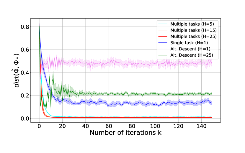
Figure 3: We plot the subspace distance between the current and ground truth representation with respect to the number of iterations, comparing between the single and multiple-task settings of Algorithm 1 and the multi-task FedRep for the IID linear regression with random covariance. We observe performance improvement and variance reduction for multi-task DFW as predicted.

Figure 3 presents a comparison of the performance between Algorithm 1 and the vanilla alternating minimization approach in both single and multi-task settings. In line with our theoretical results, the figure demonstrates that as the number of tasks $H$ increases, the error between the current representation and the ground truth representation significantly diminishes. In the specific case of linear regression with iid and non-isotropic data, this figure emphasizes that a small number of tasks ($H=5$), is sufficient to achieve a low error in computing a shared representation across the tasks. Furthermore, the depicted figure reveals that while the multi-task alternating descent algorithm outperforms the single-task case, it is worth noting that this algorithm remains sub-optimal and is unable to surpass the limitation imposed by the presence of bias in the non-isotropic data. Despite its improved performance, the multi-task alternating descent algorithm still encounters challenges in overcoming the inherent noise barrier.

C.2 System Identification

Building upon the results presented in §4, we conduct an extended experiment involving a larger range of tasks while maintaining the parameters specified in §4.2. Specifically, we generate distinct random operators different from those utilized to obtain the results illustrated in Figure 2(b). In this current analysis, we present the outcomes for the expanded range of tasks using Algorithm 1 and compare them to the single-task and multi-task vanilla alternating minimization-descent algorithms. The step-size $\eta$ is set to $1\times 10^{-1}$ for both the single-task and multi-task implementations of Algorithm 1, while for the single-task and multi-task vanilla alternating minimization-descent algorithms, we set $\eta$ to $2\times 10^{-3}$.

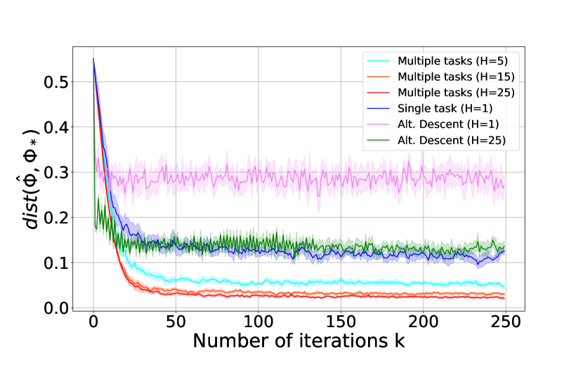
Figure 4: We plot the subspace distance between the current and ground truth representation with respect to the number of iterations, comparing between the single and multiple-task settings of Algorithm 1 multi-task FedRep for the linear system identification with random covariance. We observe performance improvement and variance reduction for multi-task DFW as predicted.

In alignment with our main theoretical findings, Figure 4 provides compelling evidence regarding the advantages of the proposed algorithm (Algorithm 1) compared to the vanilla alternating descent approach when computing a shared representation for all tasks. Consistent with the trend observed in Figure 3 for the linear regression problem, Figure 4 illustrates a significant reduction in the error between the current representation and the ground truth representation as the number of tasks increases. Additionally, it is noteworthy that while the multi-task alternating descent outperforms the single-task scenario, the single-task variant of Algorithm 1 achieves even better results. This observation underscores the importance of incorporating de-biasing and feature-whitening techniques when dealing with non-iid and non-isotropic data.

C.3 Imitation Learning

Our focus now turns to the problem of learning a linear quadratic regulator (LQR) controller, denoted as $K^{(H+1)}=F^{(H+1)}_{\star}\Phi_{\star}$, by imitating the behavior of $H$ expert controllers $K^{(1)},K^{(2)},\ldots,K^{(H)}$. These controllers share a common low-rank representation and can be decomposed into the form $K^{(h)}=F^{(h)}_{\star}\Phi_{\star}$, where $F^{(h)}_{\star}$ represents the task-specific weight and $\Phi_{\star}$ corresponds to the common representation across all tasks. To achieve this, we exploit Algorithm 1 to compute a shared low-rank representation for all tasks by leveraging data obtained from the expert controllers. Within this context, we consider a discrete-time linear time-invariant dynamical system as follows:

$$x^{(h)}[t+1]=Ax^{(h)}[t]+Bu^{(h)}[t],\;\ t=0,1,\ldots,T-1,$$

with $n_{x}=4$ states and $n_{u}=4$ inputs, for all $h\in[H+1]$, where $u^{(h)}[t]=K^{(h)}x^{(h)}[t]+z^{(h)}[t]$, with $z^{(h)}[t]\sim\mathcal{N}(0,I_{n_{u}})$ being the input noise. In our current setting, rather than directly observing the state, we obtain a high-dimensional observation derived from an injective linear function of the state. Specifically, we assume that $y^{(h)}[t]=Gx^{(h)}[t]+w^{(h)}[t]$, where $G\in\mathbb{R}^{25\times 4}$ represents the high-dimensional linear mapping. The injective linear mapping matrix $G$ is generated by applying a thin_svd operation to a random matrix with values drawn from a normal distribution $\mathcal{N}(0,1)$. This process ensures injectiveness with a high probability.

For this aforementioned multi-task imitation learning setting, we adopt a scheme in which we gather observations of the form $\{\{y^{(h)}[h],u^{(h)}[t]\}_{t=0}^{T-1}\}_{h=1}^{H}$ from the initial $H$ expert controllers to learn the controller $K^{(H+1)}$. These observations are obtained by following the dynamics:

$$y^{(h)}[t]=(\tilde{A}+\tilde{B}\tilde{K}^{(h)})y[t]+\tilde{B}z^{(h)}[t]+w^{(h)}[t]$$

with $\tilde{A}=GAG^{\dagger}$, $\tilde{B}=GB$, $\tilde{K}^{(h)}=K^{(h)}G^{\dagger}$, and process noise $w^{(h)}[t]\sim\mathcal{N}(0,\Sigma_{w})$.

The collection of stabilizing LQR controllers $K^{(1)},K^{(2)},\ldots,K^{(H+1)}$ is generated by assigning different cost matrices, namely $R=\frac{1}{4}I_{n_{u}}$ and $Q^{(h)}=\alpha^{(h)}I_{n_{x}}$, where $\alpha^{(h)}\in\texttt{logspace}(0,3,H)$. These matrices are then utilized to solve the Discrete Algebraic Ricatti Equation (DARE): $P^{(h)}=A^{\top}P^{(h)}A^{\top}+A^{\top}P^{(h)}B(B^{\top}P^{(h)}B+R)^{-1}B^{\top}P^{(h)}A+Q^{(h)}$, and compute $K^{(h)}=-(B^{\top}P^{(h)}B+R)^{-1}B^{\top}P^{(h)}A$, for all $h\in[H+1]$. Moreover, the system matrices $A$ and $B$ are randomly generated, with elements drawn from a uniform distribution. The trajectory length $T=75$ remains consistent for all tasks. The shared representation is initialized by applying a random rotation to the true representation, denoted as $\Phi_{\star}=G^{\dagger}$.

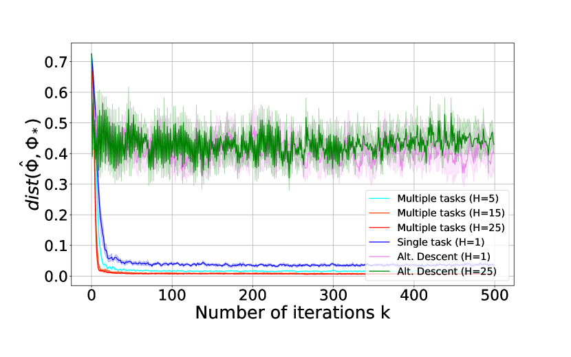
Figure 5: We plot the subspace distance between the current and ground truth representation with respect to the number of iterations, comparing between the single and multiple-task settings of Algorithm 1 and the multi-task FedRep for the imitation learning with random covariance. We observe performance improvement and variance reduction for multi-task DFW as predicted.

Figure 5 presents a comparative analysis between Algorithm 1 and the vanilla alternating minimization-descent approach (FedRep in [1]) for computing a shared representation across linear quadratic regulators. This shared representation is then utilized to derive the learned controller $K^{(H+1)}$ in a few-shot learning manner. Consistent with our theoretical findings and in alignment with the trends observed in Figures 3-4, Figure 5 demonstrates a substantial reduction in the error between the current representation and the ground truth representation when leveraging data from multiple tasks, compared to the single-task scenario in Algorithm 1. Furthermore, this figure underscores the significance of de-biasing and whitening the feature data in overcoming the bias barrier introduced by non-iid and non-isotropic data. In contrast, the vanilla alternating descent algorithm fails to address this challenge adequately and yields sub-optimal solutions.

References

- Collins et al. [2021] Liam Collins, Hamed Hassani, Aryan Mokhtari, and Sanjay Shakkottai. Exploiting shared representations for personalized federated learning. In International Conference on Machine Learning, pages 2089–2099. PMLR, 2021.
- Bullins et al. [2019] Brian Bullins, Elad Hazan, Adam Kalai, and Roi Livni. Generalize across tasks: Efficient algorithms for linear representation learning. In algorithmic learning theory, pages 235–246. PMLR, 2019.
- Du et al. [2020] Simon S Du, Wei Hu, Sham M Kakade, Jason D Lee, and Qi Lei. Few-shot learning via learning the representation, provably. arXiv preprint arXiv:2002.09434, 2020.
- Tripuraneni et al. [2021] Nilesh Tripuraneni, Chi Jin, and Michael Jordan. Provable meta-learning of linear representations. In International Conference on Machine Learning, pages 10434–10443. PMLR, 2021.
- Thekumparampil et al. [2021] Kiran Koshy Thekumparampil, Prateek Jain, Praneeth Netrapalli, and Sewoong Oh. Sample efficient linear meta-learning by alternating minimization, 2021.
- Saunshi et al. [2021] Nikunj Saunshi, Arushi Gupta, and Wei Hu. A representation learning perspective on the importance of train-validation splitting in meta-learning, 2021.
- Modi et al. [2021] Aditya Modi, Mohamad Kazem Shirani Faradonbeh, Ambuj Tewari, and George Michailidis. Joint learning of linear time-invariant dynamical systems. arXiv preprint arXiv:2112.10955, 2021.
- Chen et al. [2023] Yiting Chen, Ana M Ospina, Fabio Pasqualetti, and Emiliano Dall’Anese. Multi-task system identification of similar linear time-invariant dynamical systems. arXiv preprint arXiv:2301.01430, 2023.
- Zhang et al. [2023] Thomas T Zhang, Katie Kang, Bruce D Lee, Claire Tomlin, Sergey Levine, Stephen Tu, and Nikolai Matni. Multi-task imitation learning for linear dynamical systems. In Learning for Dynamics and Control Conference, pages 586–599. PMLR, 2023.
- Maurer et al. [2016] Andreas Maurer, Massimiliano Pontil, and Bernardino Romera-Paredes. The benefit of multitask representation learning. Journal of Machine Learning Research, 17(81):1–32, 2016.
- Teh et al. [2017] Yee Whye Teh, Victor Bapst, Wojciech Marian Czarnecki, John Quan, James Kirkpatrick, Raia Hadsell, Nicolas Heess, and Razvan Pascanu. Distral: Robust multitask reinforcement learning, 2017.
- Hessel et al. [2018] Matteo Hessel, Hubert Soyer, Lasse Espeholt, Wojciech Czarnecki, Simon Schmitt, and Hado van Hasselt. Multi-task deep reinforcement learning with popart, 2018.
- Singh et al. [2020] Avi Singh, Eric Jang, Alexander Irpan, Daniel Kappler, Murtaza Dalal, Sergey Levine, Mohi Khansari, and Chelsea Finn. Scalable multi-task imitation learning with autonomous improvement, 2020.
- Deisenroth et al. [2014] Marc Peter Deisenroth, Peter Englert, Jan Peters, and Dieter Fox. Multi-task policy search for robotics. In 2014 IEEE International Conference on Robotics and Automation (ICRA), pages 3876–3881, 2014. doi: 10.1109/ICRA.2014.6907421.
- Lu et al. [2021] Rui Lu, Gao Huang, and Simon S. Du. On the power of multitask representation learning in linear mdp, 2021.
- Cheng et al. [2022] Yuan Cheng, Songtao Feng, Jing Yang, Hong Zhang, and Yingbin Liang. Provable benefit of multitask representation learning in reinforcement learning, 2022.
- Maurer et al. [2015] Andreas Maurer, Massimiliano Pontil, and Bernardino Romera-Paredes. The benefit of multitask representation learning, 2015.
- Harrison et al. [2018] James Harrison, Apoorva Sharma, Roberto Calandra, and Marco Pavone. Control adaptation via meta-learning dynamics. In Workshop on Meta-Learning at NeurIPS, volume 2018, 2018.
- Richards et al. [2021] Spencer M Richards, Navid Azizan, Jean-Jacques Slotine, and Marco Pavone. Adaptive-control-oriented meta-learning for nonlinear systems. arXiv preprint arXiv:2103.04490, 2021.
- Shi et al. [2021] Guanya Shi, Kamyar Azizzadenesheli, Michael O’Connell, Soon-Jo Chung, and Yisong Yue. Meta-adaptive nonlinear control: Theory and algorithms. Advances in Neural Information Processing Systems, 34:10013–10025, 2021.
- Muthirayan et al. [2022] Deepan Muthirayan, Dileep Kalathil, and Pramod P Khargonekar. Meta-learning online control for linear dynamical systems. arXiv preprint arXiv:2208.10259, 2022.
- Guo et al. [2023] Taosha Guo, Abed AlRahman Al Makdah, Vishaal Krishnan, and Fabio Pasqualetti. Imitation and transfer learning for lqg control. arXiv preprint arXiv:2303.09002, 2023.
- Li et al. [2022] Lidong Li, Claudio De Persis, Pietro Tesi, and Nima Monshizadeh. Data-based transfer stabilization in linear systems. arXiv preprint arXiv:2211.05536, 2022.
- Wang et al. [2022] Han Wang, Leonardo F Toso, and James Anderson. Fedsysid: A federated approach to sample-efficient system identification. arXiv preprint arXiv:2211.14393, 2022.
- Xin et al. [2023] Lei Xin, Lintao Ye, George Chiu, and Shreyas Sundaram. Learning dynamical systems by leveraging data from similar systems. arXiv preprint arXiv:2302.04344, 2023.
- Faradonbeh and Modi [2022] Mohamad Kazem Shirani Faradonbeh and Aditya Modi. Joint learning-based stabilization of multiple unknown linear systems. IFAC-PapersOnLine, 55(12):723–728, 2022.
- Mitra et al. [2021] Aritra Mitra, Rayana Jaafar, George J. Pappas, and Hamed Hassani. Linear convergence in federated learning: Tackling client heterogeneity and sparse gradients, 2021.
- Jain et al. [2021] Prateek Jain, John Rush, Adam Smith, Shuang Song, and Abhradeep Guha Thakurta. Differentially private model personalization. Advances in Neural Information Processing Systems, 34:29723–29735, 2021.
- Bietti et al. [2022] Alberto Bietti, Chen-Yu Wei, Miroslav Dudik, John Langford, and Steven Wu. Personalization improves privacy-accuracy tradeoffs in federated learning. In International Conference on Machine Learning, pages 1945–1962. PMLR, 2022.
- Kulkarni et al. [2020] Viraj Kulkarni, Milind Kulkarni, and Aniruddha Pant. Survey of personalization techniques for federated learning. In 2020 Fourth World Conference on Smart Trends in Systems, Security and Sustainability (WorldS4), pages 794–797. IEEE, 2020.
- Luo et al. [2021] Mi Luo, Fei Chen, Dapeng Hu, Yifan Zhang, Jian Liang, and Jiashi Feng. No fear of heterogeneity: Classifier calibration for federated learning with non-iid data, 2021.
- Yang et al. [2023] Lei Yang, Jiaming Huang, Wanyu Lin, and Jiannong Cao. Personalized federated learning on non-iid data via group-based meta-learning. ACM Trans. Knowl. Discov. Data, 17(4), mar 2023. ISSN 1556-4681. doi: 10.1145/3558005. URL https://doi.org/10.1145/3558005.
- McMahan et al. [2023] H. Brendan McMahan, Eider Moore, Daniel Ramage, Seth Hampson, and Blaise Agüera y Arcas. Communication-efficient learning of deep networks from decentralized data, 2023.
- Zhu et al. [2021] Hangyu Zhu, Jinjin Xu, Shiqing Liu, and Yaochu Jin. Federated learning on non-iid data: A survey, 2021.
- Ma et al. [2022] Xiaodong Ma, Jia Zhu, Zhihao Lin, Shanxuan Chen, and Yangjie Qin. A state-of-the-art survey on solving non-iid data in federated learning. Future Generation Computer Systems, 135:244–258, 2022.
- Stewart and Sun [1990] Gilbert W Stewart and Ji-guang Sun. Matrix perturbation theory. Academic press, 1990.
- Petersen et al. [2008] Kaare Brandt Petersen, Michael Syskind Pedersen, et al. The matrix cookbook. Technical University of Denmark, 7(15):510, 2008.
- Trefethen and Bau [2022] Lloyd N Trefethen and David Bau. Numerical linear algebra, volume 181. Siam, 2022.
- LeCun et al. [2002] Yann LeCun, Léon Bottou, Genevieve B Orr, and Klaus-Robert Müller. Efficient backprop. In Neural networks: Tricks of the trade, pages 9–50. Springer, 2002.
- Abbasi-Yadkori et al. [2011] Yasin Abbasi-Yadkori, Dávid Pál, and Csaba Szepesvári. Online least squares estimation with self-normalized processes: An application to bandit problems. arXiv preprint arXiv:1102.2670, 2011.
- Abbasi-Yadkori [2013] Yasin Abbasi-Yadkori. Online learning for linearly parametrized control problems. 2013.
- Hsu et al. [2012] Daniel Hsu, Sham M Kakade, and Tong Zhang. Random design analysis of ridge regression. In Conference on learning theory, pages 9–1. JMLR Workshop and Conference Proceedings, 2012.
- Yu [1994] Bin Yu. Rates of convergence for empirical processes of stationary mixing sequences. The Annals of Probability, pages 94–116, 1994.
- Mohri and Rostamizadeh [2008] Mehryar Mohri and Afshin Rostamizadeh. Rademacher complexity bounds for non-iid processes. Advances in Neural Information Processing Systems, 21, 2008.
- Kuznetsov and Mohri [2017] Vitaly Kuznetsov and Mehryar Mohri. Generalization bounds for non-stationary mixing processes. Machine Learning, 106(1):93–117, 2017.
- Tsiamis et al. [2022a] Anastasios Tsiamis, Ingvar Ziemann, Nikolai Matni, and George J Pappas. Statistical learning theory for control: A finite sample perspective. arXiv preprint arXiv:2209.05423, 2022a.
- Collins et al. [2023] Liam Collins, Hamed Hassani, Mahdi Soltanolkotabi, Aryan Mokhtari, and Sanjay Shakkottai. Provable multi-task representation learning by two-layer relu neural networks. arXiv preprint arXiv:2307.06887, 2023.
- Meunier et al. [2023] Dimitri Meunier, Zhu Li, Arthur Gretton, and Samory Kpotufe. Nonlinear meta-learning can guarantee faster rates, 2023.
- Sarkar et al. [2021] Tuhin Sarkar, Alexander Rakhlin, and Munther A Dahleh. Finite time lti system identification. The Journal of Machine Learning Research, 22(1):1186–1246, 2021.
- Tu and Recht [2018] Stephen Tu and Benjamin Recht. Least-squares temporal difference learning for the linear quadratic regulator. In International Conference on Machine Learning, pages 5005–5014. PMLR, 2018.
- Tropp [2011] Joel A. Tropp. User-friendly tail bounds for sums of random matrices. Foundations of Computational Mathematics, 12(4):389–434, aug 2011. doi: 10.1007/s10208-011-9099-z. URL https://doi.org/10.1007%2Fs10208-011-9099-z.
- Horn and Johnson [2012] Roger A Horn and Charles R Johnson. Matrix analysis. Cambridge university press, 2012.
- Hu et al. [2023] Bin Hu, Kaiqing Zhang, Na Li, Mehran Mesbahi, Maryam Fazel, and Tamer Başar. Toward a theoretical foundation of policy optimization for learning control policies. Annual Review of Control, Robotics, and Autonomous Systems, 6:123–158, 2023.
- Krauth et al. [2019] Karl Krauth, Stephen Tu, and Benjamin Recht. Finite-time analysis of approximate policy iteration for the linear quadratic regulator. Advances in Neural Information Processing Systems, 32, 2019.
- Tu and Recht [2019] Stephen Tu and Benjamin Recht. The gap between model-based and model-free methods on the linear quadratic regulator: An asymptotic viewpoint. In Conference on Learning Theory, pages 3036–3083. PMLR, 2019.
- Recht [2019] Benjamin Recht. A tour of reinforcement learning: The view from continuous control. Annual Review of Control, Robotics, and Autonomous Systems, 2:253–279, 2019.
- Fazel et al. [2018] Maryam Fazel, Rong Ge, Sham Kakade, and Mehran Mesbahi. Global convergence of policy gradient methods for the linear quadratic regulator. In International Conference on Machine Learning, pages 1467–1476. PMLR, 2018.
- Simchowitz and Foster [2020] Max Simchowitz and Dylan Foster. Naive exploration is optimal for online lqr. In International Conference on Machine Learning, pages 8937–8948. PMLR, 2020.
- Dean et al. [2018] Sarah Dean, Horia Mania, Nikolai Matni, Benjamin Recht, and Stephen Tu. Regret bounds for robust adaptive control of the linear quadratic regulator. Advances in Neural Information Processing Systems, 31, 2018.
- Dean et al. [2020] Sarah Dean, Horia Mania, Nikolai Matni, Benjamin Recht, and Stephen Tu. On the sample complexity of the linear quadratic regulator. Foundations of Computational Mathematics, 20(4):633–679, 2020.
- Agarwal et al. [2019a] Naman Agarwal, Elad Hazan, and Karan Singh. Logarithmic regret for online control. Advances in Neural Information Processing Systems, 32, 2019a.
- Agarwal et al. [2019b] Naman Agarwal, Brian Bullins, Elad Hazan, Sham Kakade, and Karan Singh. Online control with adversarial disturbances. In International Conference on Machine Learning, pages 111–119. PMLR, 2019b.
- Ziemann et al. [2022] Ingvar Ziemann, Anastasios Tsiamis, Henrik Sandberg, and Nikolai Matni. How are policy gradient methods affected by the limits of control? In 2022 IEEE 61st Conference on Decision and Control (CDC), pages 5992–5999. IEEE, 2022.
- Ziemann and Sandberg [2022] Ingvar Ziemann and Henrik Sandberg. Regret lower bounds for learning linear quadratic gaussian systems. arXiv preprint arXiv:2201.01680, 2022.
- Lee et al. [2023] Bruce D Lee, Ingvar Ziemann, Anastasios Tsiamis, Henrik Sandberg, and Nikolai Matni. The fundamental limitations of learning linear-quadratic regulators. arXiv preprint arXiv:2303.15637, 2023.
- Simchowitz et al. [2018] Max Simchowitz, Horia Mania, Stephen Tu, Michael I Jordan, and Benjamin Recht. Learning without mixing: Towards a sharp analysis of linear system identification. In Conference On Learning Theory, pages 439–473. PMLR, 2018.
- Tsiamis et al. [2022b] Anastasios Tsiamis, Ingvar M Ziemann, Manfred Morari, Nikolai Matni, and George J Pappas. Learning to control linear systems can be hard. In Conference on Learning Theory, pages 3820–3857. PMLR, 2022b.
- Jedra and Proutiere [2020] Yassir Jedra and Alexandre Proutiere. Finite-time identification of stable linear systems optimality of the least-squares estimator. In 2020 59th IEEE Conference on Decision and Control (CDC), pages 996–1001, 2020. doi: 10.1109/CDC42340.2020.9304362.
- Tu et al. [2022] Stephen Tu, Roy Frostig, and Mahdi Soltanolkotabi. Learning from many trajectories. arXiv preprint arXiv:2203.17193, 2022.
- Goldenshluger and Zeevi [2001] Alexander Goldenshluger and Assaf Zeevi. Nonasymptotic bounds for autoregressive time series modeling. The Annals of Statistics, 29(2):417–444, 2001.