How to harness high-dimensional temporal entanglement, using limited interferometry setups.

Abstract

High-dimensional entanglement has shown to have significant advantages in quantum communication. It is available in many degrees of freedom and in particular in the time-domain routinely produced in down-conversion (SPDC). While advantageous in the sense that only a single detector channel is needed locally, it is notoriously hard to analyze, especially in an assumption-free manner that is required for quantum key distribution applications. We develop the first complete analysis of high-dimensional entanglement in the polarization-time-domain and show how to efficiently certify relevant density matrix elements and security parameters for Quantum Key Distribution (QKD). In addition to putting past experiments on rigorous footing, we also develop physical noise models and propose a novel setup that can further enhance the noise resistance of free-space quantum communication.

I Introduction

Secure and secret communication is a fundamental pillar of modern society. Quantum communication, exploring the potential of using quantum mechanical carriers of information, is one of the maturest quantum technologies available today. One of the principal applications is the establishment of (inherently secret) quantum-mechanical correlations over long distances, which can then be used to perform e.g. quantum key distribution (QKD) [1, 2]. Such an entanglement distribution faces severe challenges, with two dominant approaches pursued. Connections via optical fibres experience exponential loss, which without genuine quantum repeaters severely limits the distance [3]. Free-space links have a more favourable loss-profile, but require direct line of sight and are limited to times of very low background noise, hence are effectively confined to nighttime operations. For long-distance satellite links this presents a heavy reduction of potential links and up-times. High-Dimensional (HD) entanglement [4, 5, 6, 7, 8] emerged as a promising solution, effectively counteracting noise-vulnerability [9], with high-dimensional entanglement in the time-domain [10] being its most promising implementation for free-space applications. Previous work has successfully demonstrated the feasibility and advantages of high dimensions in entanglement distribution [11, 12, 13]. Data analysis methods in these complex setups, however, were primarily heuristic and relied on assumptions that are not suitable for adversarial scenarios and thus could lead to security vulnerabilities in entanglement-based quantum cryptography.

In this Letter, we provide a rigorous theoretical analysis of an experimental setup designed for distribution of high-dimensional entanglement suitable for High-Dimensional Quantum Key Distribution (HD QKD) with photons entangled in both polarization and time. We also propose a new and slightly altered scheme that eliminates all assumptions on the entagled states made in previous work. Additionally, we demonstrate that under a realistic noise model the new setup is able to produce secure key for almost twice as many solar photons as the previously analyzed schemes, without relying on restrictive assumptions, opening the path towards full daylight quantum key distribution in free-space setups.

II Setting

The analyzed high-dimensional QKD setup is built upon two identical measurement devices which are placed in the communicating parties’ labs as well as an entangled photon pair source which can be placed either in one of both parties’ labs or in the middle and does not need to be trusted. We define the parties’ time-reference points via synchronised coincidence windows, that will henceforth be called time-frames. In case the source is placed in one of the parties’ labs, the delay in arrival time in comparison to the lab of the second party is accounted for, i.e., the time-reference points of detection are brought into agreement.
The source is aimed to produce general polarized, time-entangled photon pairs in $\left(\mathcal{H}_{\textrm{Pol}}\otimes\mathcal{H}_{T}\right)^{\otimes 2}$,

$$\ket{\Psi_{\textrm{target}}^{\textrm{ideal}}}:=\sum_{p\in\mathcal{P}}\int_{0}^{\infty}\int_{0}^{\infty}\Psi(p,t)\ket{p,t,t^{\prime}}~{}\textrm{d}\mu(t,t^{\prime}),$$

where $\mu(t)$ is some appropriate measure and $\mathcal{P}:=\{HH,HV,VH,VV\}$. Here, $\mathcal{H}_{\textrm{Pol}}$ is a two-dimensional Hilbert space representing the polarization degree of freedom, while, in principle, we require an infinite-dimensional Hilbert space $\mathcal{H}_{T}$ to represent the temporal degree of freedom. However, any realistic time-resolving photon measurement discretizes the temporal degree of freedom into detection events of finitely many time-bins.
Let us call $T>0$, chosen such that $\Psi(t)$ is sufficiently close to zero outside the interval $[0,T]$, time frame length and let $d$ be the number of time-bins. Consequently, the length of a single time-bin is given by $t_{B}:=\frac{T}{d}$. Hence, effectively, we require a $d$-dimensional Hilbert space $\mathcal{H}_{T}$ to capture the temporal aspects of the photons under consideration. Then, our effective target state reads

$$\ket{\Psi_{\textrm{target}}^{\textrm{eff}}}:=\sum_{p\in\mathcal{P}}c_{p}\ket{p}\otimes\frac{1}{\sqrt{d}}\sum_{k=0}^{d-1}\ket{kk},$$ (1)

where $c_{p}\in\mathbb{C}$ with $\sum_{p}|c_{p}|^{2}=1$. The single shares of the photon pair are transmitted to Alice and Bob, respectively.

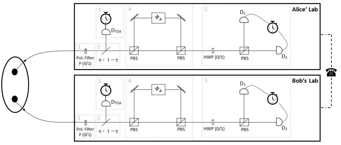
Figure 1: Sketch of the analysed setup. A photon source prepares entangled photons and sends them to two identical labs. Each of the labs is equipped with a polarizing filter (1) which can be either inserted (Protocol 1) or removed (Protocol 2). Then a beam splitter (2) allows to choose between two measurements. In (3), a time-resolving photon detector allows to measure the arrival time of incoming photons. In the second measurement setup (4,5), two polarizing beamsplitters (PBS) and two mirrors allow to superpose neighboring time-bins. Finally, a half-wave plate (HWP) that can be either inserted or removed together with another PBS and two time-resolving photon detectors allow to perform time-superposition measurements. Furthermore, both labs are connected via a classical channel, allowing to exchange authenticated classical messages.

Each of their labs is equipped with a measurement setup, comprised out of five major components (see Figure 1), (1) a polarization filter, (2) an $\eta:1-\eta$ beam splitter, (3) a detector setup in one of the BS arms, and (4) an interferometer with (5) an additional measurement apparatus in the other BS arm. The polarization filter (1) can be set to an arbitrary orientation or can be removed completely. The following $\eta:1-\eta$ beam splitter (2) allows to passively switch between two measurement setups. In one arm (3), there is a time-resolving photon detector that records the arrival time of the incoming photons. Consequently, measurements in this arm are referred to as measurements in the Time-of-Arrival (ToA) basis. In the other arm, there is a Franson-interferometer [14] setup (4,5) that allows to measure the temporal superposition of neighboring time-bins, referred to as measurements in the Temporal-Superposition (TSUP) basis. There, the incident light meets the first polarizing beam splitter (PBS) of the interferometer. Horizontally polarized components of the light are transmitted while vertically polarized components are reflected and take the long path of the interferometer. We adjust the long interferometer arm to cause a time-delay of one time-bin. However, we emphasize that this is just a choice and our analysis holds for general time-delays. Additionally, a phase-shifter allows to modify the phase of the part of the signal taking the long path. After being reflected by two mirrors, the two components meet again at the second PBS. Note that now vertically polarized light with time-stamp $i-1$ meets horizontally polarized light with time-stamp $i$, due to the delay caused by the long interferometer arm. Finally, the merged beams enter the measurement device (5). There, the light passes a half-wave plate which rotates the polarization axis of the incident light by $45^{\circ}$ before meeting another polarizing beam splitter. In each of the outputs of the PBS, a click detector which is connected to a clock records incoming photons and their arrival times. This allows us to measure a superposition of neighboring time-bins (with or without a complex phase between them – depending on the setting of the phase-shifter). We note that the same measurements can also be realized with active choice instead of the beamsplitter in (2), such that both measurements are performed with only two detectors. For simplicity, we analyse the passive choice setup, however, the following analysis is also valid for active basis choice.

III Measurements

While it is straight-forward to see that for the ToA basis the measurement operator for each party has the form $M^{A/B}:=\mathbbm{1}_{\textrm{Pol}}\otimes\ket{i}\!\bra{i}$, we show in Appendix A that the measurement in the Franson setup (i.e. in the TSUP basis) can be replaced by a projection onto one out of two states, depending on which detector clicks,

$$\ket{\Psi_{1}^{A/B}\left(i,\phi^{A/B}\right)} :=\frac{\ket{H}{\ket{i}}+e^{-i\phi^{A/B}}\ket{V}\ket{i-1}}{\sqrt{2}},$$ (2)

$$\ket{\Psi_{2}^{A/B}\left(i,\phi^{A/B}\right)} :=\frac{\ket{H}{\ket{i}}-e^{-i\phi^{A/B}}\ket{V}\ket{i-1}}{\sqrt{2}},$$ (3)

where the indices $A$ and $B$ denote Alice’s and Bob’s part respectively and the indices $1$ and $2$ the two detectors. These measurements with time-stamp $i$ correspond to POVM elements associated with the detection time of a photon emitted at time $t_{i}$ that travelled the short interferometer path. While previous work assumed that the polarization degree of freedom remains unchanged while passing through the quantum channel, generally, Alice and Bob obtain a quantum state $\rho\in\mathcal{D}\left(\left(\mathcal{H}_{\textrm{Pol}}\otimes\mathcal{H}_{T}\right)^{\otimes 2}\right)$. Both record time-stamped clicks and correlate the ones within the temporal margin of the time-frame as coincidence click-matrices

$$\textrm{CC}(i,j):=\#\text{Clicks per frame in time-bin $i$ and $j$}.$$ (4)

In general, they obtain four different kinds of click-matrices that we are going to label as follows: TT if both measure in the ToA basis, SS if both measure in the TSUP basis, TS if Alice measures in the ToA and Bob in the TSUP basis, and ST if Alice measures in the TSUP and Bob in the ToA basis. Then, the respective coincidence click matrices are normalized $\textrm{TT}(i,j):=\frac{\textrm{CC}(i,j)}{\sum_{k,l}\textrm{CC}(k,l)}$ and can be related to the following POVM elements

$$\textrm{TT}(i,j) :=\mathrm{Tr}\left[\rho\left(M^{A}(i)\otimes M^{B}(j)\right)\right],$$ (5)

$$\textrm{SS}_{a,b}(i,j) :=\mathrm{Tr}\left[\rho\left(\tilde{M}^{A}_{a}(i,\phi^{A})\otimes\tilde{M}^{B}_{b}(j,,\phi^{B})\right)\right],$$ (6)

$$\textrm{TS}_{b}(i,j) :=\mathrm{Tr}\left[\rho\left(M^{A}(i)\otimes\tilde{M}^{B}_{b}(j,\phi^{B})\right)\right],$$ (7)

$$\textrm{ST}_{a}(i,j) :=\mathrm{Tr}\left[\rho\left(\tilde{M}^{A}_{a}(i,\phi^{A})\otimes M^{B}(j,\phi^{B})\right)\right],$$ (8)

where $\tilde{M}^{A}_{a}(i,\phi^{A}):=\outerproduct{\Psi_{a}^{A}(i,\phi^{A})}{\Psi_{a}^{A}(i,\phi^{A})}$ and $\tilde{M}^{B}_{b}(j,\phi^{B}):=\outerproduct{\Psi_{b}^{B}(j,\phi^{B})}{\Psi_{b}^{B}(j,\phi^{B})}$, for $a,b\in\{1,2\}$ indicating which detector clicks and $i,j\in\{0,...,d-1\}$ marking the time-stamps on each side. While we have specified the state prepared by the source, the state Alice and Bob receive is unknown, as in QKD the channel connecting Alice and Bob is assumed to possibly be fully under control of an eavesdropper, called Eve. By performing measurements, Alice and Bob aim to certify that the temporal part of their shared state is entangled and decoupled from Eve’s part.

In general, the interpretation of the measurements and their meaning for the time-part of the density matrix depends on the polarization degree of freedom of the state Alice and Bob receive. A common approach so far has been to assume (a) that temporal and polarization degrees of freedom are actually independent from each other, i.e. $\rho=\rho_{\textrm{Pol}}\otimes\rho_{T}$ and (b) that the polarization degree of freedom does not change while the photons travel through the quantum channel. The assumed perfect knowledge of the polarization degree of freedom has allowed to directly interpret the measurements’ effect on the time-part of the density matrix. Alternatively, one could lift assumption (b) by performing state-tomography of the polarization density matrix by adding and using an additional measurement arm at the cost of losing a certain fraction of the signals and making the analysis significantly more complicated.

In what follows, we propose a solution that simultaneously removes both assumptions (a) and (b) while at the same time improves the noise-resistance of the setup and eases the practical complexity of the experiment significantly. As shown in Figure 1, we suggest adding an additional polarization filter set to let $D$-polarized photons pass at the entrance of both Alice’s and Bob’s lab before the signal meets the first beamsplitter. Thus, compared to earlier setups [13], we can replace the whole ToA measurement by one time-resolving photon detector (and remove the additional measurement arm, which is required to perform tomography of the polarization density matrix). While this simple modification eases the experimental setup considerably, by forcing Alice’s and Bob’s joint state to be $\outerproduct{DD}{DD}\otimes\rho_{T}$ after the polarization filter we are able to go without any assumptions about the internal structure of the state that enters the lab and without requiring that only the time-part is manipulated while passing the quantum channel. Furthermore, we expect our proposed protocol to be more favourable in the finite-size regime as well as we need to account finite-size effects for fewer measurements. We take our proposed protocol as an example to illustrate our method (details can be found in Appendix B.1, but analysis of all mentioned (and a plethora of unmentioned) variants work similarly. We also analyse a protocol similar to that used in [12, 13] (see Appendix B.2) and compare both protocols.

Summing up, Alice and Bob measure clicks with respect to either a time-of-arrival or a time-superposition measurement. Naturally, each of the clicks corresponds to a projective measurement on the incoming quantum signal, which we can use to build three independent POVMs. To see this, we first rewrite Eqs. (2) and (3) to obtain

$$\ket{\Psi_{1}^{A/B}\left(i,\phi^{A/B}\right)} =\frac{\ket{D}{\ket{i+}}+\ket{A}\ket{i-}}{\sqrt{2}},$$ (9)

$$\ket{\Psi_{2}^{A/B}\left(i,\phi^{A/B}\right)} =\frac{\ket{D}{\ket{i-}}+\ket{A}\ket{i+}}{\sqrt{2}},$$ (10)

where

$$\ket{i\pm}:=\frac{1}{\sqrt{2}}\left(\ket{i}\pm e^{-i\phi^{A/B}}\ket{i-1}\right).$$ (11)

While the action of ToA directly yields the diagonal of the time-density matrix

$$\textrm{TT}(i,j)\propto\innerproduct{i,j|\rho_{T}}{i,j},$$ (12)

for the TSUP measurement we obtain

$$\textrm{SS}_{1,1}(i,j) \propto\innerproduct{i+,j+|\rho_{T}}{i+,j+},$$ (13)

$$\textrm{SS}_{1,2}(i,j) \propto\innerproduct{i+,j-|\rho_{T}}{i+,j-},$$ (14)

$$\textrm{SS}_{2,1}(i,j) \propto\innerproduct{i-,j+|\rho_{T}}{i-,j+},$$ (15)

$$\textrm{SS}_{2,2}(i,j) \propto\innerproduct{i-,j-|\rho_{T}}{i-,j-},$$ (16)

which can be used to obtain off diagonal elements of $\rho$ (see [13]). For the mismatched measurements we obtain similar mixed expressions of the form

$$\textrm{ST}_{a}(i,j) \propto\innerproduct{i+,j|\rho_{T}}{i+,j},$$ (17)

$$\textrm{TS}_{b}(i,j) \propto\innerproduct{i,j+|\rho_{T}}{i,j+}.$$ (18)

For simplicity we assume that $d$ is even in what follows, in order to explain how these click-matrices can be interpreted. We want to emphasize that our method is not limited to this case and that this choice is solely made for illustration purposes and generalizes straight-forwardly to arbitrary dimensions.

Note that the right-hand sides of the click-equations are composed out of matrix elements of the time-density matrix. It can be seen directly that the ToA clicks (TT) already correspond to a POVM, giving rise to a basis $\mathcal{B}_{0}:=\mathcal{B}_{0}^{A}\otimes\mathcal{B}_{0}^{B}$, where $\mathcal{B}_{0}^{A/B}:=\left\{\ket{i}\right\}_{i=0}^{d-1}$ spans single time-bin subspaces. In contrast, the TSUP measurements can be used to construct even two POVM measurements. For the first of the two corresponding bases, $\mathcal{B}_{1}:=\mathcal{B}_{1}^{A}\otimes\mathcal{B}_{1}^{B}$, notice that $\ket{i\pm}$ for fixed $i$ spans two-dimensional time-bin subspaces. Thus, we first consider odd $i$ and obtain $\mathcal{B}_{1}^{A/B}:=\left\{\ket{(2k-1)\pm}\right\}_{k=1}^{\frac{d}{2}}$ as a basis for Alice’s, respectively Bob’s, $d$-dimensional temporal Hilbert space. For the last basis, $\mathcal{B}_{2}:=\mathcal{B}_{2}^{A}\otimes\mathcal{B}_{2}^{B}$, we consider even $i$. Based on our measurement setup we are not able to directly measure elements spanning the boundary subspaces $\textrm{span}\{\ket{0}\}$ and $\textrm{span}\{\ket{d-1}\}$ in the TSUP basis with even $i$ and hence need to substitute them by combinations of elements where the parties have used different measurements (so, the TS- and ST-clicks). We obtain $\mathcal{B}_{2}^{A/B}:=\{\ket{(2k)\pm}\}_{k=1}^{\frac{d}{2}-1}\cup\left\{\ket{0},\ket{d-1}\right\}$. This translation of projective measurements on $\left(\mathcal{H}_{\textrm{Pol}}\otimes\mathcal{H}_{T}\right)^{\otimes 2}$ resulting in coincidence-click-matrices to POVM elements on only the temporal Hilbert space allows us now to normalize the click-matrices correctly. Finally, we want to emphasize the importance of the overlap between the subspaces spanned by $\mathcal{B}_{1}$ and $\mathcal{B}_{2}$, which allows to certify high-dimensional entanglement.

IV Quantum Key Distribution

Having clarified the setting, let us discuss one possible application, namely High-Dimensional (HD) Discrete-Variable (DV) Quantum Key Distribution (QKD). Therefore, Alice and Bob execute the following protocol.

1. State Preparation— A source generates photon pairs entangled in polarization and time (see Eq. (1)) and sends them to Alice and Bob.

2. Measurement— Alice and Bob each perform a ToA measurement or a TSUP measurement, depending on independent random bits $\mathbb{P}_{A/B}\in\{0,1\}$. This step can be implemented passively via a beamsplitter.

Steps 1) and 2) are repeated $N$-times, where $N$ is assumed to be very large.

1. Announcement & Sifting— Alice and Bob publicly announce their measurement choices for every round via the classical channel and sift rounds where they have performed different measurements.

2. Parameter Estimation & Key Generation— Next, they disclose some of their results from measurements of each basis to perform statistical tests. If the tests are passed, they use the ToA measurements to create a common raw key by performing a key map, where logical bit-values are assigned to the measurement results. Otherwise they abort the protocol and start again at step 1).

3. Error-correction & Privacy Amplification— By means of classical algorithms Alice and Bob reconcile their raw keys and perform privacy amplification to eliminate potential eavesdroppers knowledge about the key.

It is known that the asymptotic secure key rate $R^{\infty}$ of a QKD protocol is lower-bounded by the Devetak-Winter bound [15]:

$$R^{\infty}\geq S(A|E)-H(A|B),$$ (19)

where $S(A|E)$ is the conditional von Neumann entropy of Alice’s key register given Eve’s quantum register, quantifying the amount of information not known by Eve and $H(A|B)$ is the Shannon entropy between Alice’s and Bob’s raw key, representing the amount of information leaked during the error-correction phase of the protocol. While the latter quantity can be easily calculated from the observed statistics, to obtain the first, we have to minimize over all quantum states $\rho_{ABE}$ compatible with Alice’s and Bob’s observations. Therefore, we use a method developed in [16] recently to obtain the first term by solving a semi-definite program (SDP), hence finding a lower bound on the secure key rate.

Results— We develop a realistic noise model (see Appendix C) taking photon losses, background noise induced by solar photons, detector inefficiencies and dark counts into account and illustrate our method by comparing secure key rates for two different protocols. In the first (‘new’) protocol, we set the source to prepare the state

$$\ket{\Psi_{1}}=\ket{DD}\otimes\frac{1}{\sqrt{d}}\sum_{k=0}^{d-1}\ket{kk}.$$ (20)

Alice and Bob each add a polarization filter, which is set to $D$, right after the photon enters their respective lab, such that they are aligned on polarization of the target state. Consequently, as outlined earlier, the state after the polarization filter has the form $\rho_{AB}=\outerproduct{DD}{DD}\otimes\rho_{T}$. We want to highlight that neither the form of the polarization part, nor the tensor product structure are mere assumptions as they are enforced by the filter. This allows a direct and clean analysis of the QKD setup without any additional, unjustified assumptions. For comparison, we also analyze a second protocol, which was already discussed in earlier work such as [12] and [13]. There, the source produces the target state

$$\ket{\Psi_{2}}=\frac{\ket{HH}+\ket{VV}}{\sqrt{2}}\otimes\frac{1}{\sqrt{d}}\sum_{k=0}^{d-1}\ket{kk}.$$ (21)

Consequently, we cannot put any polarization filter in the entry of Alice’s resp. Bob’s lab. Now either we have to assume that (a) the polarization remains unchanged over the channel (which is a very strong assumption) and still forms a tensor product with the time-part, which means Alice’s and Bob’s shared state is of the form

$$\rho_{AB}=$$

$$\frac{\outerproduct{HH}{HH}+\ket{HH}\!\!\bra{VV}+\ket{VV}\!\!\bra{HH}+\outerproduct{VV}{VV}}{2}\otimes\rho_{T},$$

or (b) that the received state has at least tensor-product structure, $\rho_{AB}=\rho_{\textrm{Pol}}\otimes\rho_{T}\in\mathcal{D}(\mathcal{H}_{\textrm{Pol}}^{\otimes 2}\otimes\mathcal{H}_{T}^{\otimes 2})$ (an as well unjustified assumption), where $\rho_{\textrm{Pol}}$ might have changed over the channel, which allows to determine the incoming $\rho_{\textrm{Pol}}$ by performing a tomography. Therefore, the key rates we obtain for this setting are only upper bounds, as under the mentioned assumptions they only treat a special case and not the general one. Since performing state tomography introduces additional uncertainties and requires additional testing, the upper bound we obtain from (b) can only be lower than the bound we obtain from (a). We therefore choose to compare Protocol 1 with variant (a) of Protocol 2. Details regarding this comparison can be found in Appendix A. Besides allowing a clean and rigorous analysis without any assumptions, we intuitively expect the additional polarization filter to increase the resistance against solar photons, which are the main source of noise in free-space and satellite QKD applications, as half of the unpolarized solar photons are blocked, while (in the ideal case) none or (in reality) only a small fraction of the source photons are.

For our simulations, we used specific parameter values in accordance with the Free-Space Link experiment between Vienna and Bisamberg [12, 13]. The length of a time frame was set to $T_{0}:=5.4\times 10^{-9}s$, the dark-count rate to $100/s$, the detection efficiency to $\eta_{D}=90\%$, the channel loss to $P_{\textrm{loss}}=99.7\%$ and the pair production rate to $0.1$ per time-frame. Consistent with the experiment, we assume that the photon source is located in Alice’s lab, meaning that channel loss only affects Bob’s quantum signals. In Figure 2, we present the secure key rates obtained for both analyzed protocols for time-dimensions of $d=4,6,8$ and $10$. Our new protocol (Protocol 1) consistently exhibits significantly higher key rates compared to the existing protocol (Protocol 2), especially as the number of solar photons increases. Additionally, Protocol 1 demonstrates an impressive tolerance to nearly twice as many solar photons per second as Protocol 2, leading to substantially enhanced noise tolerance and practicality. It is crucial to note that the curves presented for Protocol 2 rely on unjustified assumptions (see our earlier analysis), serving as mere upper bounds, while the analysis of Protocol 1 avoids these assumptions, offering reliable lower bounds. This advantage makes the performance difference between the two protocols even more striking.

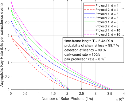
Figure 2: Comparison between old (dashed line) and new protocol for various dimensions.

V Discussion

Given that the analysed setup was able to transmit key during early daytime in summer [12] in urban atmospheric conditions, the seemingly modest increase of a factor of almost 2 in solar photons is actually significantly closing the gap towards a full-day operation. Notwithstanding further technical improvements as sharper frequency filters, adaptive optics to correct for atmospheric turbulences, we are thus hopeful that the presented setup is both simple enough to practically build without great challenges, as only one interferometer needs to be stabilised per site. At first glance it may seem counterintuitive that intereference between neighbouring bins can reveal anything more than analysing the same setup as time-bin qubits. The fact that a time-bin has interference with both neighbouring bins, however, reveals that nothing but a genuinely higher-dimensional state is compatible with the measurement outcomes and so opens up the possibility to utilise larger portions of the discretised Hilbert space than just binarizations (time-bin qubits). One should note that our key rates are of course asymptotic and for the finite key-analysis it will be crucial to get data on the rate of change and the actual required splitting ratio between TSUP and ToA measurements to collect a sufficient amount of data in both. Furthermore, for an online analysis of outcomes, potentially switching optimal dimensionality according to current conditions, we will need to relax the full SDP constraint we are currently using and switch to rapidly computable quantifiers of the security parameter directly.

VI Conclusion

Our present work has closed the gap in literature of a clean and rigorous analysis of a high-dimensional QKD setup for polarization-time-bin entanglement, highlighting implicit assumptions in previous settings and suggesting a simple and efficient modification to remove these assumptions. Moreover, we have demonstrated that our novel modification also helps to increase the protocol’s noise-resistance against solar photons by a factor of almost two, which is a significant step towards closing the last gaps in all-day operations for global satellite networks.

Appendix A Analysis of the Franson Setup

Recall from the main part that, effectively, the quantum system on each side can be described in a Hilbert space $\mathcal{H}^{A/B}=\mathcal{H}_{\textrm{Pol}}\otimes\mathcal{H}_{T}$. For ease of notation, we define $d:=\dim(\mathcal{H}_{T})$. Possible bases for $\mathcal{H}_{\textrm{Pol}}$ are given by $\{\ket{H},\ket{V}\}$ and $\{\ket{D},\ket{A}\}$, where the first set of basis vectors corresponds to horizontally and vertically polarized photons, while the second set corresponds to diagonally and anti-diagonally polarized ones. Furthermore, a basis of $\mathcal{H}_{T}$ is given by the time-bin states $\{\ket{n}\}_{n=0}^{d-1}$. This allows us to define the time-shift operation by its action on basis states, $\hat{T}:\mathcal{H}_{T}\rightarrow\mathcal{H}_{T},~{}\ket{n}\mapsto\ket{n+1}$. Additionally, we can define the phase-shift operator $\hat{Q}_{\phi}:\mathcal{H}_{\textrm{Pol}}\otimes\mathcal{H}_{T}\rightarrow\mathcal{H}_{\textrm{Pol}}\otimes\mathcal{H}_{T},~{}\ket{p,n}\rightarrow e^{i\phi}\ket{p,n}$. After having introduced this notation, we can start describing the action of the measurement setup. Let $\rho_{AB}\in\mathcal{D}\left(\mathcal{H}^{A}\otimes\mathcal{H}^{B}\right)$ be the joint quantum state that enters Alice’s and Bob’s lab. The action of the Time-of-Arrival (ToA) measurement setup on this state is straightforward, as a detection event at time $i$ simply corresponds to a projection of the incoming state onto $\ket{i}$. Thus, the corresponding measurement operator reads

$$M(i)=\mathbbm{1}_{\textrm{Pol}}\otimes\outerproduct{i}{i}.$$ (22)

In what follows, we discuss the corresponding operators for Time-Superposition measurements.

Denote by $x$ and $y$ the horizontal and vertical input port of a polarizing beam splitter respectively and by $x^{\prime}$ and $y^{\prime}$ the corresponding outputs. Note that in our setup, the first beam splitter has only one input port and the second beam splitter has only one output port. Then, the action of a PBS is given by the unitary

$$\hat{U}_{\textrm{PBS}}=\left(\ket{H}\!\!\bra{H}\otimes\ket{x^{\prime}}\!\!\bra{x}+\ket{V}\!\!\bra{V}\otimes\ket{x^{\prime}}\!\!\bra{y}+\ket{V}\!\!\bra{H}\otimes\ket{y^{\prime}}\!\!\bra{x}+\ket{V}\!\!\bra{V}\otimes\ket{y^{\prime}}\!\!\bra{y}\right)\otimes\mathbbm{1}_{T}.$$ (23)

According to the description of our measurement setup above, only those parts in the upper $y^{\prime}$-part experience a time- as well as a phase-shift. Thus, let

$$\hat{T}_{y} :=\mathbbm{1}_{\textrm{Pol}}\otimes\mathbbm{1}_{T}\otimes\ket{x^{\prime}}\!\!\bra{x^{\prime}}+\mathbbm{1}_{\textrm{Pol}}\otimes\hat{T}\otimes\ket{y^{\prime}}\!\!\bra{y^{\prime}}$$ (24)

$$\hat{Q}_{y} :=\mathbbm{1}_{\textrm{Pol}}\otimes\mathbbm{1}_{T}\otimes\ket{x^{\prime}}\!\!\bra{x^{\prime}}+\hat{Q}_{\phi}\otimes\ket{y^{\prime}}\!\!\bra{y^{\prime}}$$ (25)

be the operators describing these shifts. They allow us to describe the action of the whole setup by applying them one after another in the correct order

$$\hat{U}_{I}:=\hat{U}_{\textrm{PBS}}\hat{Q}_{y}\hat{T}_{y}\hat{U}_{\textrm{PBS}}.$$ (26)

As the output of the first PBS is directed to the input of the second PBS, we simply write $(x^{\prime},y^{\prime})$ for the input ports of the second PBS, while we proceed with $(x^{\prime\prime},y^{\prime\prime})$ for its outputs. We obtain

$$\hat{U}_{I}=\left(\ket{H}\!\!\bra{H}\otimes\mathbbm{1}_{T}+\ket{V}\!\!\bra{V}\otimes\hat{Q}_{\phi}\hat{T}\right)\otimes\ket{x^{\prime\prime}}\!\!\bra{x}+\left(\ket{H}\!\!\bra{H}\otimes\hat{Q}_{\phi}\hat{T}+\ket{V}\!\!\bra{V}\otimes\mathbbm{1}_{T}\right)\otimes\ket{y^{\prime\prime}}\!\!\bra{y}.$$ (27)

Note that in our case input $y$ is empty, so effectively we only need to consider the first term – horizontally polarized states pass the interferometer untouched while vertically polarized states experience a time- as well as a phase-shift. As we put our measurement devices in the output port $x^{\prime\prime}$ of the interferometer, we can drop the register $x^{\prime\prime}$ for ease of notation.

Finally, we obtain the unitary operator representing the action of the whole measurement setup on Alice’s and Bob’s joint state $\rho_{AB}$,

$$\begin{aligned} \hat{U}&:=\hat{U}_{I}\otimes\hat{U}_{I}\\ &=\ket{HH}\!\!\bra{HH}\otimes\mathbbm{1}_{T}\otimes\mathbbm{1}_{T}+\ket{HV}\!\!\bra{HV}\otimes\mathbbm{1}_{T}\otimes\hat{Q}_{\phi}\hat{T}+\ket{VH}\!\!\bra{VH}\otimes\hat{Q}_{\phi}\hat{T}\otimes\mathbbm{1}_{T}+\ket{VV}\!\!\bra{VV}\otimes\hat{Q}_{\phi}\hat{T}\otimes\hat{Q}_{\phi}\hat{T}.\end{aligned}$$ (28)

The interferometer is followed by a half-wave plate and another polarizing beam splitter, followed by two detectors, one in each arm of the PBS such that the right detector measures horizontally polarized photons, while the upper detector measures vertically polarized photons. However, the half-wave plate rotates the plane of polarization as $U_{\textrm{HWP}}\ket{H}=\ket{D}$ and $U_{\textrm{HWP}}\ket{V}=\ket{A}$, i.e., it allows us to measure diagonally polarized photons in the right arm and anti-diagonally polarized photons in the upper arm. The corresponding measurements project onto $\ket{D,i}$ and $\ket{A,i}$ respectively.

To ease our examination, we want to find the ‘effective’ measurement parts 4 and 5 (see Figure 1) perform on our input state $\rho_{AB}$, i.e., if $O$ denotes the measurement we perform on the state $\rho_{\textrm{out}}$ that has passed the Franson setup, we aim to find $\tilde{O}:=\outerproduct{\tilde{\Psi}}{\tilde{\Psi}}$ such that

$$\mathrm{Tr}\left[\rho_{AB}\tilde{O}\right]=\mathrm{Tr}\left[\rho_{\textrm{out}}O\right]=\mathrm{Tr}\left[\hat{U}\rho_{AB}\hat{U}^{\dagger}O\right]=\mathrm{Tr}\left[\rho_{AB}\hat{U}^{\dagger}O\hat{U}\right].$$ (29)

Hence, we obtain the effective measurement operator via $\tilde{O}=\hat{U}^{\dagger}O\hat{U}$,

$$\hat{U}^{\dagger}\ket{DD,i,j} =\ket{\tilde{\Psi}_{+}(i,\phi_{A})}\otimes\ket{\tilde{\Psi}_{+}(j,\phi_{B})}=:\ket{\tilde{\Psi}_{1}(i,j,\phi_{A},\phi_{B})},$$ (30)

$$\hat{U}^{\dagger}\ket{DA,i,j} =\ket{\tilde{\Psi}_{+}(i,\phi_{A})}\otimes\ket{\tilde{\Psi}_{-}(j,\phi_{B})}=:\ket{\tilde{\Psi}_{2}(i,j,\phi_{A},\phi_{B})},$$ (31)

$$\hat{U}^{\dagger}\ket{AD,i,j} =\ket{\tilde{\Psi}_{-}(i,\phi_{A})}\otimes\ket{\tilde{\Psi}_{+}(j,\phi_{B})}=:\ket{\tilde{\Psi}_{3}(i,j,\phi_{A},\phi_{B})},$$ (32)

$$\hat{U}^{\dagger}\ket{AA,i,j} =\ket{\tilde{\Psi}_{-}(i,\phi_{A})}\otimes\ket{\tilde{\Psi}_{-}(j,\phi_{B})}=:\ket{\tilde{\Psi}_{4}(i,j,\phi_{A},\phi_{B})},$$ (33)

where we have defined

$$\ket{\tilde{\Psi}_{\pm}(i,\phi)} :=\frac{1}{\sqrt{2}}\left(\ket{H,i}\pm e^{-i\phi}\ket{V,i-1}\right)=\frac{1}{\sqrt{2}}\left(\ket{D}\otimes\frac{\ket{i}\pm e^{-i\phi}\ket{i-1}}{\sqrt{2}}+\ket{A}\otimes\frac{\ket{i}\mp e^{-i\phi}\ket{i-1}}{\sqrt{2}}\right).$$ (34)

Appendix B QKD Protocols

Next, we discuss different examples for how this setup can be used to establish QKD protocols. In each of the protocols, Alice and Bob each apply measurements either in the ToA or in the TSUP setting, producing coincidence-clicks which are recorded in different coincidence-click-matrices. If Alice’s and Bob’s detectors $a$ and $b$ click with time-stamps $i$ and $j$ respectively, depending on which measurements they chose, they record these events according to the following notation.

• If both measured the time of arrival, the corresponding coincidence-click element is $\textrm{TT}(i,j)$.

• If both performed the time-superposition measurement, the corresponding coincidence-click element is $\textrm{SS}_{a,b}(i,j)$.

• If Alice measured ToA while Bob measured TSUP, the corresponding coincidence-click element is $\textrm{TS}_{b}(i,j)$.

• If Alice measured TSUP while Bob measured ToA, the corresponding coincidence-click element is $\textrm{ST}_{a}(i,j)$.

Note that we only need to record which detector clicked if the measurement was performed in the TSUP setting, as clicks in the ToA setting do not discriminate polarization. With the quantities derived in Appendix A, we obtain

$$\textrm{TT}(i,j) =\mathrm{Tr}\left[\rho_{AB}\left(\mathbbm{1}_{\textrm{Pol}}^{\otimes 2}\otimes\outerproduct{i,j}{i,j}\right)\right]$$ (35)

$$\textrm{SS}_{1,1}(i,j) =\mathrm{Tr}\left[\rho_{AB}\outerproduct{\tilde{\Psi}_{1}(i,j,\phi_{A},\phi_{B})}{\tilde{\Psi}_{1}(i,j,\phi_{A},\phi_{B})}\right]$$ (36)

$$\textrm{SS}_{1,2}(i,j) =\mathrm{Tr}\left[\rho_{AB}\outerproduct{\tilde{\Psi}_{2}(i,j,\phi_{A},\phi_{B})}{\tilde{\Psi}_{2}(i,j,\phi_{A},\phi_{B})}\right]$$ (37)

$$\textrm{SS}_{2,1}(i,j) =\mathrm{Tr}\left[\rho_{AB}\outerproduct{\tilde{\Psi}_{3}(i,j,\phi_{A},\phi_{B})}{\tilde{\Psi}_{3}(i,j,\phi_{A},\phi_{B})}\right]$$ (38)

$$\textrm{SS}_{2,2}(i,j) =\mathrm{Tr}\left[\rho_{AB}\outerproduct{\tilde{\Psi}_{4}(i,j,\phi_{A},\phi_{B})}{\tilde{\Psi}_{4}(i,j,\phi_{A},\phi_{B})}\right]$$ (39)

$$\textrm{TS}_{1}(i,j) =\mathrm{Tr}\left[\rho_{AB}\left(\left(\mathbbm{1}_{\textrm{Pol}}\otimes\outerproduct{i}{i}\right)\otimes\outerproduct{\tilde{\Psi}_{+}(j,\phi_{B})}{\tilde{\Psi}_{+}(j,\phi_{B})}\right)\right]$$ (40)

$$\textrm{TS}_{2}(i,j) =\mathrm{Tr}\left[\rho_{AB}\left(\left(\mathbbm{1}_{\textrm{Pol}}\otimes\outerproduct{i}{i}\right)\otimes\outerproduct{\tilde{\Psi}_{-}(j,\phi_{B})}{\tilde{\Psi}_{-}(j,\phi_{B})}\right)\right]$$ (41)

$$\textrm{ST}_{1}(i,j) =\mathrm{Tr}\left[\rho_{AB}\left(\outerproduct{\tilde{\Psi}_{+}(i,\phi_{A})}{\tilde{\Psi}_{+}(i,\phi_{A})}\otimes{\left(\mathbbm{1}_{\textrm{Pol}}\otimes\outerproduct{j}{j}\right)}\right)\right]$$ (42)

$$\textrm{ST}_{2}(i,j) =\mathrm{Tr}\left[\rho_{AB}\left(\outerproduct{\tilde{\Psi}_{-}(i,\phi_{A})}{\tilde{\Psi}_{-}(i,\phi_{A})}\otimes{\left(\mathbbm{1}_{\textrm{Pol}}\otimes\outerproduct{j}{j}\right)}\right)\right].$$ (43)

B.1 Protocol 1 ($\ket{DD}$)

We set the source to produce the target state $\ket{\Psi_{\textrm{target}}}=\ket{DD}\otimes\frac{1}{\sqrt{d}}\sum_{k=0}^{d-1}\ket{kk}$. Since this state then travels through the quantum channel, which is assumed to possibly be under Eve’s control, we do not know anything about the structure of the state once its shares arrive in Alice’s and Bob’s labs. Therefore, we place a polarizing filter in each of the labs which is set to $D$. Consequently, independently of what happens to the state in the quantum channel, after the filter Alice’s and Bob’s joint quantum state $\rho_{AB}$ reads $\ket{DD}\otimes\rho_{T}$, where $\rho_{T}$ is an arbitrary quantum state in $\mathcal{H}_{T}$. While each of the recorded coincidence-clicks corresponds to a projective measurement on $\mathcal{H}_{\textrm{Pol}}\otimes\mathcal{H}_{T}$, to find the correct normalisation, we aim to build POVMs on the time-part only.

For the ToA measurements, it follows directly that the coincidence-clicks correspond to the diagonal entries of the time-density matrix,

$$\textrm{TT}(i,j)=\bra{i,j|\rho_{T}}\ket{i,j}.$$ (44)

For the TSUP measurements, using the $D/A$ representation from Eq. (34), we obtain

$$\textrm{SS}_{1,1}(i,j) =\frac{1}{4}\bra{i+,j+|\rho_{T}}\ket{i+,j+},$$ (45)

$$\textrm{SS}_{1,2}(i,j) =\frac{1}{4}\bra{i+,j-|\rho_{T}}\ket{i+,j-},$$ (46)

$$\textrm{SS}_{2,1}(i,j) =\frac{1}{4}\bra{i-,j+|\rho_{T}}\ket{i-,j+},$$ (47)

$$\textrm{SS}_{2,2}(i,j) =\frac{1}{4}\bra{i-,j-|\rho_{T}}\ket{i-,j-},$$ (48)

where $\ket{i\pm}$ and $\ket{j\pm}$ are defined as in Eq. (11). Note that these click-events have a direct physical interpretation. If on both sides detector $1$ clicks, this means both have measured a positive phase between two neighbouring time-bins labelled by $i$ and $j$, while clicks of detector $2$ on both sides indicate a negative phase. If opposite detectors click, this indicates that they have measured different phases between neighbouring time-bins.

Finally, the mismatched measurements yield

$$\textrm{TS}_{1}(i,j) =\frac{1}{2}\bra{i,j+|\rho_{T}}\ket{i,j+},$$ (49)

$$\textrm{TS}_{2}(i,j) =\frac{1}{2}\bra{i,j-|\rho_{T}}\ket{i,j-},$$ (50)

$$\textrm{ST}_{1}(i,j) =\frac{1}{2}\bra{i+,j|\rho_{T}}\ket{i+,j},$$ (51)

$$\textrm{ST}_{2}(i,j) =\frac{1}{2}\bra{i-,j|\rho_{T}}\ket{i-,j}.$$ (52)

One sees immediately that

$$\mathcal{M}_{0}^{P1}:=\left\{\outerproduct{i,j}{i,j}\right\}_{i,j=0}^{d-1}$$ (53)

is a POVM induced by the bases $\mathcal{B}_{0}^{A/B}$ on Alice’s and Bob’s side, respectively, with corresponding click-matrix

$$C_{\mathcal{M}_{0}^{P1}}(i,j):=\textrm{TT}(i,j),$$ (54)

where we use the natural order $\{\ket{0},\ket{1},\ldots,\ket{d-1}\}$. Furthermore, it can be checked easily that

$$\mathcal{M}_{1}^{P1}:=\left\{\outerproduct{i+,j+}{i+,j+},\outerproduct{i+,j-}{i+,j-},\outerproduct{i-,j+}{i-,j+},\outerproduct{i-,j-}{i-,j-}\right\}_{i,j\textrm{ odd}}$$ (55)

forms another POVM, induced by the bases $\mathcal{B}_{1}^{A/B}$ on Alice’s and Bob’s side, respectively. The corresponding click-matrix reads

$$\begin{aligned} &C_{\mathcal{M}_{1}^{P1}}:=\\ &4\begin{pmatrix}\textrm{SS}_{1,1}(1,1)&\textrm{SS}_{1,2}(1,1)&\textrm{SS}_{1,1}(1,3)&\textrm{SS}_{1,2}(1,3)&\ldots&\textrm{SS}_{1,1}(1,d-1)&\textrm{SS}_{1,2}(1,d-1)\\ \textrm{SS}_{2,1}(1,1)&\textrm{SS}_{2,2}(1,1)&\textrm{SS}_{2,1}(1,3)&\textrm{SS}_{2,2}(1,3)&\ldots&\textrm{SS}_{2,1}(1,d-1)&\textrm{SS}_{2,2}(1,d-1)\\ \textrm{SS}_{1,1}(3,1)&\textrm{SS}_{1,2}(3,1)&\textrm{SS}_{1,1}(3,3)&\textrm{SS}_{1,2}(3,3)&\ldots&\textrm{SS}_{1,1}(3,d-1)&\textrm{SS}_{1,2}(3,d-1)\\ \textrm{SS}_{2,1}(3,1)&\textrm{SS}_{2,2}(3,1)&\textrm{SS}_{2,1}(3,3)&\textrm{SS}_{2,2}(3,3)&\ldots&\textrm{SS}_{2,1}(3,d-1)&\textrm{SS}_{2,2}(3,d-1)\\ \vdots&\vdots&\vdots&\vdots&\ddots&\vdots&\vdots\\ \textrm{SS}_{1,1}(d-1,1)&\textrm{SS}_{1,2}(d-1,1)&\textrm{SS}_{1,1}(d-1,3)&\textrm{SS}_{1,2}(d-1,3)&\ldots&\textrm{SS}_{1,1}(d-1,d-1)&\textrm{SS}_{1,2}(d-1,d-1)\\ \textrm{SS}_{2,1}(d-1,1)&\textrm{SS}_{2,2}(d-1,1)&\textrm{SS}_{2,1}(d-1,3)&\textrm{SS}_{2,2}(d-1,3)&\ldots&\textrm{SS}_{2,1}(d-1,d-1)&\textrm{SS}_{2,2}(d-1,d-1)\\ \end{pmatrix},\end{aligned}$$ (56)

where we have ordered the basis vectors $\{\ket{1+},\ket{1-},\ket{3+},\ket{3-},\ldots,\ket{(d-1)+},\ket{(d-1)-}\}$. Finally, we argue that by combining clicks from different measurements, we can form a third POVM,

$$\mathcal{M}_{2}^{P1}:=\left\{\outerproduct{i\pm,j\pm}{i\pm,j\pm}\right\}_{i,j>0,\textrm{ even}}\cup\left\{\outerproduct{i,j\pm}{i,j\pm}\right\}_{{i\in\{0,d-1\}}\atop{j>0,\textrm{ even }}}\cup\left\{\outerproduct{i\pm,j}{i\pm,j}\right\}_{{i>0,\textrm{ even }}\atop{j\in\{0,d-1\}}}\cup\left\{\outerproduct{i,j}{i,j}\right\}_{i,j\in\{0,d-1\}},$$ (57)

which is induced by the bases $\mathcal{B}_{2}^{A/B}$ on Alice’s and Bob’s side, respectively. The corresponding click-matrix reads

$$\begin{aligned} &C_{\mathcal{M}_{2}^{P1}}:=\\ &\begin{pmatrix}\textrm{TT}(0,0)&2\textrm{TS}_{1}(0,2)&2\textrm{TS}_{2}(0,2)&2\textrm{TS}_{1}(0,4)&2\textrm{TS}_{2}(0,4)&\ldots&\textrm{TT}(0,d-1)\\ 2\textrm{ST}_{1}(2,0)&4\textrm{SS}_{1,1}(2,2)&4\textrm{SS}_{1,2}(2,2)&4\textrm{SS}_{1,1}(2,4)&4\textrm{SS}_{1,2}(2,4)&\ldots&2\textrm{ST}_{1}(2,d-1)\\ 2\textrm{ST}_{2}(2,0)&4\textrm{SS}_{2,1}(2,2)&4\textrm{SS}_{2,2}(2,2)&4\textrm{SS}_{2,1}(2,4)&4\textrm{SS}_{2,2}(2,4)&\ldots&2\textrm{ST}_{2}(2,d-1)\\ 2\textrm{ST}_{1}(4,0)&4\textrm{SS}_{1,1}(4,2)&4\textrm{SS}_{1,2}(4,2)&4\textrm{SS}_{1,1}(4,4)&4\textrm{SS}_{1,2}(4,4)&\ldots&2\textrm{ST}_{1}(4,d-1)\\ 2\textrm{ST}_{2}(4,0)&4\textrm{SS}_{2,1}(4,2)&4\textrm{SS}_{2,2}(4,2)&4\textrm{SS}_{2,1}(4,4)&4\textrm{SS}_{2,2}(4,4)&\ldots&2\textrm{ST}_{2}(4,d-1)\\ \vdots&\vdots&\vdots&\vdots&\vdots&\ddots&\vdots\\ 2\textrm{ST}_{2}(d-3,0)&4\textrm{SS}_{2,1}(d-3,2)&4\textrm{SS}_{2,2}(d-3,2)&4\textrm{SS}_{2,1}(d-3,4)&4\textrm{SS}_{2,2}(d-3,4)&\ldots&2\textrm{ST}_{2}(d-3,d-1)\\ \textrm{TT}(d-1,0)&2\textrm{TS}_{1}(d-1,2)&2\textrm{TS}_{2}(d-1,2)&2\textrm{TS}_{1}(d-1,4)&2\textrm{TS}_{2}(d-1,4)&\ldots&\textrm{TT}(d-1,d-1)\end{pmatrix},\end{aligned}$$ (58)

where the order of the basis vectors is $\{\ket{0},\ket{2+}\ket{2-},\ldots,\ket{(d-3)+},\ket{(d-3)-},\ket{d-1}\}$. Note that the different weight-factors ensure correct normalisation of the click-matrix.

B.2 Protocol 2 ($\ket{HH}+\ket{VV}$)

Finally, we come to the second protocol where the target state is $\ket{\Psi_{\textrm{target}}}=\frac{\ket{HH}+\ket{VV}}{\sqrt{2}}\otimes\frac{1}{\sqrt{d}}\sum_{k=0}^{d-1}\ket{kk}$. Unlike in Protocol 1, there is no polarization filter, so we have to assume that the polarization remains unchanged when the state passes the quantum channel. Thus, Alice’s and Bob’s shared state reads $\rho_{AB}=\frac{\ket{HH}\!\bra{HH}+\ket{HH}\!\bra{VV}+\ket{VV}\!\bra{HH}+\ket{VV}\!\bra{VV}}{2}\otimes\rho_{T}$. Like for Protocol 1, it follows directly that the coincidence-clicks for the ToA-measurements correspond to the diagonal entries of the time-density matrix,

$$\textrm{TT}(i,j)=\bra{i,j|\rho_{T}}\ket{i,j}.$$ (59)

Applying Eqs. (36) - (39) to $\rho_{AB}$ yields

$$\textrm{SS}_{1,1}(i,j) =\frac{1}{8}\left(\bra{i+,j+|\rho_{T}}\ket{i+,j+}+\innerproduct{i+,j+|\rho_{T}}{i-,j-}+\innerproduct{i-,j-|\rho_{T}}{i+,j+}+\innerproduct{i-,j-|\rho_{T}}{i-,j-}\right)$$ (60)

$$=\textrm{SS}_{2,2}(i,j),$$ (61)

$$\textrm{SS}_{1,2}(i,j) =\frac{1}{8}\left(\bra{i+,j-|\rho_{T}}\ket{i+,j-}+\innerproduct{i+,j-|\rho_{T}}{i-,j+}+\innerproduct{i-,j+|\rho_{T}}{i+,j-}+\innerproduct{i-,j-|\rho_{T}}{i-,j-}\right)$$ (62)

$$=\textrm{SS}_{2,1}(i,j).$$ (63)

As $\textrm{SS}_{1,1}(i,j)$ and $\textrm{SS}_{2,2}(i,j)$ as well as $\textrm{SS}_{1,2}(i,j)$ and $\textrm{SS}_{2,1}(i,j)$ are equal, we can combine those elements respectively to ’same phase‘ and ’opposite phase‘ clicks,

$$\textrm{SS}_{s}(i,j) :=\textrm{SS}_{1,1}(i,j)+\textrm{SS}_{2,2}(i,j)$$ (64)

$$\textrm{SS}_{o}(i,j) :=\textrm{SS}_{1,2}(i,j)+\textrm{SS}_{2,1}(i,j).$$ (65)

For the mismatched measurements, we obtain from Eqs. (40)-(43)

$$\textrm{TS}_{1}(i,j) =\frac{1}{2}\bra{i,j+|\rho_{T}}\ket{i,j+},$$ (66)

$$\textrm{TS}_{2}(i,j) =\frac{1}{2}\bra{i,j-|\rho_{T}}\ket{i,j-},$$ (67)

$$\textrm{ST}_{1}(i,j) =\frac{1}{2}\bra{i+,j|\rho_{T}}\ket{i+,j},$$ (68)

$$\textrm{ST}_{2}(i,j) =\frac{1}{2}\bra{i-,j|\rho_{T}}\ket{i-,j}.$$ (69)

Like for Protocol 1, one can see immediately that

$$\mathcal{M}_{0}^{P1}:=\left\{\outerproduct{i,j}{i,j}\right\}_{i,j=0}^{d-1}$$ (70)

forms a POVM induced by the bases $\mathbbm{B}_{0}^{A/B}$ on Alice’s and Bob’s side respectively with corresponding click-matrix

$$C_{\mathcal{M}_{0}^{P1}}(i,j):=\textrm{TT}(i,j),$$ (71)

where we have chosen the natural order $\{\ket{0},\ket{1},...,\ket{d-1}\}$. Next, we aim to find a second POVM, which requires some preparations. From the definitions made in Eqs. (64) and (65), it follows directly that

$$\textrm{SS}_{s}(i,j) =\frac{1}{2}\mathrm{Tr}\left[\rho_{T}\outerproduct{\Phi^{A,B}_{s}(i,j)}{\Phi^{A,B}_{s}(i,j)}\right]$$ (72)

$$\textrm{SS}_{o}(i,j) =\frac{1}{2}\mathrm{Tr}\left[\rho_{T}\outerproduct{\Phi^{A,B}_{o}(i,j)}{\Phi^{A,B}_{o}(i,j)}\right],$$ (73)

with

$$\ket{\Phi^{A,B}_{s}(i,j)}:=\frac{1}{\sqrt{2}}\left(\ket{i+,j+}+\ket{i-,j-}\right),$$ (74)

$$\ket{\Phi^{A,B}_{o}(i,j)}:=\frac{1}{\sqrt{2}}\left(\ket{i+,j-}+\ket{i-,j+}\right).$$ (75)

A short calculation shows that

$$\outerproduct{\Phi^{A,B}_{s}(i,j)}{\Phi^{A,B}_{s}(i,j)}+\outerproduct{\Phi^{A,B}_{o}(i,j)}{\Phi^{A,B}_{o}(i,j)}=\outerproduct{i,j}{i,j}+\outerproduct{i-1,j-1}{i-1,j-1}$$

and

$$\outerproduct{i,j+}{i,j+}+\outerproduct{i,j-}{i,j-} =\outerproduct{i,j}{i,j}+\outerproduct{i,j-1}{i,j-1}$$

$$\outerproduct{i+,j}{i+,j}+\outerproduct{i-,j}{i-,j} =\outerproduct{i,j}{i,j}+\outerproduct{i-1,j}{i-1,j}.$$

Next, we combine those measurement operators and obtain

$$\sum_{i,j=1}^{d-1}\left(\outerproduct{\Phi^{A,B}_{s}(i,j)}{\Phi^{A,B}_{s}(i,j)}+\outerproduct{\Phi^{A,B}_{o}(i,j)}{\Phi^{A,B}_{o}(i,j)}\right)$$

$$+ \sum_{j=1}^{d-1}\left(\outerproduct{0,j+}{0,j+}+\outerproduct{0,j-}{0,j-}+\outerproduct{d-1,j+}{d-1,j+}+\outerproduct{d-1,j-}{d-1,j-}\right)$$

$$+ \sum_{i=1}^{d-1}\left(\outerproduct{i+,0}{i+,0}+\outerproduct{i-,0}{i-,0}+\outerproduct{i+,d-1}{i+,d-1}+\outerproduct{i-,d-1}{i-,d-1}\right)$$

$$+ \left(\mathbbm{1}_{d\times d}-\outerproduct{00}{00}-\outerproduct{d-1,d-1}{d-1,d-1}\right)$$

$$= 3\mathbbm{1}_{d\times d}.$$

Thus, after scaling all elements with $\frac{1}{3}$, we obtain the second POVM,

$$\mathcal{M}_{1}^{P2}:= \left\{\frac{1}{3}\left(\mathbbm{1}_{d\times d}-\outerproduct{00}{00}-\outerproduct{d-1,d-1}{d-1,d-1}\right),\frac{1}{3}\outerproduct{\Phi^{A,B}_{s}(i,j)}{\Phi^{A,B}_{s}(i,j)},\frac{1}{3}\outerproduct{\Phi^{A,B}_{o}(i,j)}{\Phi^{A,B}_{o}(i,j)},\right.$$ (76)

$$~{}~{}~{}\frac{1}{3}\outerproduct{0,j+}{0,j+},\frac{1}{3}\outerproduct{0,j-}{0,j-},\frac{1}{3}\outerproduct{d-1,j+}{d-1,j+},\frac{1}{3}\outerproduct{d-1,j+}{d-1,j+},$$

$$~{}~{}\left.\frac{1}{3}\outerproduct{i+,0}{i+,0},\frac{1}{3}\outerproduct{i-,0}{i-,0},\frac{1}{3}\outerproduct{i+,d-1}{i+,d-1},\frac{1}{3}\outerproduct{i-,d-1}{i-,d-1}\right\}_{i,j=1}^{d-1}.$$

Consequently, taking both the renormalisation by $\frac{1}{3}$ and Eqs. (64) - (69) into account, the corresponding clicks are normalized as follows,

$$1 =\frac{1}{3}\left(1-\textrm{TT}(0,0)-\textrm{TT}(d-1,d-1)\right)+\frac{2}{3}\sum_{i,j=1}^{d-1}\left(\textrm{SS}_{s}(i,j)+\textrm{SS}_{o}(i,j)\right)$$ (77)

$$+\frac{2}{3}\sum_{j=1}^{d-1}\left(\textrm{TS}_{1}(0,j)+\textrm{TS}_{2}(0,j)+\textrm{TS}_{1}(d-1,j)+\textrm{TS}_{2}(d-1,j)\right)$$

$$+\frac{2}{3}\sum_{i=1}^{d-1}\left(\textrm{ST}_{1}(i,0)+\textrm{ST}_{2}(i,0)+\textrm{ST}_{1}(i,d-1)+\textrm{ST}_{2}(i,d-1)\right).$$

As we have already used the clicks from the computational basis measurement (TT-clicks), we do not expect any contribution to the key rates from these clicks. Since they simply introduce redundant constraints into our semi-definite program, we can remove those elements/clicks when we formulate the SDP as long as we account for them during normalisation.

Contrary to Protocol 1, we have already exhausted our measurements such that we cannot build a third POVM.

Appendix C Noise Model

As already mentioned in the main text, similarly as in [11] and [18] we have to consider various origins of noise. In particular, there are noise effects due to the interaction of the photons with the environment, mainly photons coming from the sun, and due to the imperfect detectors, so we take into account four different kinds of imperfections:

• Channel loss: Photons might get lost on the way from the source to the labs.

• Detection inefficiency: Due to detection inefficiencies, incoming photons cause a click with probability $\eta_{D}\in[0,1]$.

• Environmental photons: Photons coming from the residual environment (like those coming from the sun) can cause clicks.

• Dark counts: Imperfections of the detectors can cause clicks even in the absence of photons.

Let $P_{\textrm{prod}}(n)$ be the probability distribution of $n$ polarized photon pairs produced by the source per time frame, let $P_{\textrm{loss}}^{A}$ and $P_{\textrm{loss}}^{B}$ denote the probabilities for source photons to get lost on their way from the source to Alice’s and Bob’s lab, respectively, and let $\eta_{A}$ and $\eta_{B}$ be the detection efficiency parameters of Alice’s and Bob’s detectors respectively. The probability that the environment, including the sun, produces $n$ (unpolarized) photons per time frame on Alice’s side is given by $P_{\textrm{env}}^{A}(n)$ and on Bob’s side by $P_{\textrm{env}}^{B}(n)$. In case the incoming photons pass a polarization filter which is aligned with the polarization produced by the source (Protocol 1), on average half of the (unpolarized) environmental photons are blocked. Moreover, for each of the detectors, $n$ dark counts per time frame may occur with a probability of $P_{\textrm{dark}}(n)$. These considerations yield:

• The probability that per time frame $T$ $n$ photon pairs are produced is given by $P_{\textrm{prod}}(n)$.

• Some photons get lost, so the probability of having $b_{1}$ respectively $b_{2}$ photons left for Alice and Bob after the lossy channel is given by

  $$P_{1}^{A}(b_{1}) =\sum_{i=b_{1}}^{\infty}P_{\textrm{prod}}(i)(1-P_{\textrm{loss}}^{A})^{b_{1}}P_{\textrm{loss}}^{i-b_{1}}\binom{i}{b_{1}},$$

  $$P_{1}^{B}(b_{2}) =\sum_{i=b_{2}}^{\infty}P_{\textrm{prod}}(i)(1-P_{\textrm{loss}}^{B})^{b_{2}}P_{\textrm{loss}}^{i-b_{2}}\binom{i}{b_{2}}$$

  respectively. These remaining photons are still polarized.

• The probability for $q$ sunlight and further environmental photons being produced within one time frame $T$ on Alice’s and Bob’s side is $P_{\textrm{env}}^{A}(q)$ and $P_{\textrm{env}}^{B}(q)$, respectively.

• When the photons pass the polarization filter (which is placed only in protocol 1), photons coming from the source remain mainly untouched, while half of the photons stemming from the sun get blocked. Therefore, the probabilities that $e_{1}$ respectively $e_{2}$ environmental photons pass Alice’s and Bob’s PBS are given by

  $$P_{\textrm{env}}^{\prime A}(e_{1}) =\sum_{j=e_{1}}^{\infty}P_{\textrm{env}}^{A}(j)\left(\frac{1}{2}\right)^{e_{1}}\ \left(1-\frac{1}{2}\right)^{j-e_{1}}\binom{j}{e_{1}}=\sum_{j=e_{1}}^{\infty}\binom{j}{e_{1}}\left(\frac{1}{2}\right)^{j}P_{\textrm{env}}^{A}(j),$$

  $$P_{\textrm{env}}^{\prime B}(e_{2}) =\sum_{j=e_{2}}^{\infty}\binom{j}{e_{2}}\left(\frac{1}{2}\right)^{j}P_{\textrm{env}}^{B}(j)$$

  respectively.

• Now the environmental photons are combined with the photons coming from the source. The probability of having $f_{1}$ photons in Alice’s lab after the polarization filter therefore is given by

  $$P_{2}^{A}(f_{1}) =\sum_{l=0}^{f_{1}}P_{1}^{A}(l)P_{\textrm{env}}^{\prime A}(f_{1}-l)$$

  $$=\sum_{l=0}^{f_{1}}\sum_{i=l}^{\infty}P_{\textrm{prod}}(i)(1-P_{\textrm{loss}}^{A})^{l}(P_{\textrm{loss}}^{A})^{(i-l)}\binom{i}{l}\sum_{j=f_{1}-l}^{\infty}\binom{j}{f_{1}-l}\left(\frac{1}{2}\right)^{j}P_{\textrm{env}}^{A}(j)$$

  $$=\sum_{l=0}^{f_{1}}\sum_{i=l}^{\infty}\sum_{j=f_{1}-l}^{\infty}\binom{i}{l}\binom{j}{f_{1}-l}P_{\textrm{prod}}(i)P_{\textrm{env}}^{A}(j)(1-P_{\textrm{loss}}^{A})^{l}(P_{\textrm{loss}}^{A})^{(i-l)}\left(\frac{1}{2}\right)^{j}$$

  and similarly for Bob the probability for having $f_{2}$ photons in his lab after the filter is

  $$P_{2}^{B}(f_{2}) =\sum_{l=0}^{f_{2}}\sum_{i=l}^{\infty}\sum_{j=f_{2}-l}^{\infty}\binom{i}{l}\binom{j}{f_{2}-l}P_{\textrm{prod}}(i)P_{\textrm{env}}^{B}(j)(1-P_{\textrm{loss}}^{B})^{l}(P_{\textrm{loss}}^{B})^{(i-l)}\left(\frac{1}{2}\right)^{j}.$$

  Since the source produces photon pairs, the joint probability for Alice and Bob to have $n_{1}$ and $n_{2}$ photons respectively after the filter is found to be

  $$P(n_{1},n_{2})=\sum_{s=0}^{\infty}\sum_{m_{1}=0}^{\min\{s,n_{1}\}}\sum_{m_{2}=0}^{\min\{s,n_{2}\}}P_{\textrm{prod}}(s) (1-P_{\textrm{loss}}^{A})^{m_{1}}(P_{\textrm{loss}}^{A})^{(s-m_{1})}\binom{s}{m_{1}}$$ (78)

  $$\cdot (1-P_{\textrm{loss}}^{B})^{m_{2}}(P_{\textrm{loss}}^{B})^{(s-m_{2})}\binom{s}{m_{2}}P_{\textrm{env}}^{\prime A}(n_{1}-m_{1})P_{\textrm{env}}^{\prime B}(n_{2}-m_{2})$$ (79)

  $$=\sum_{s=0}^{\infty}\sum_{m_{1}=0}^{\min\{s,n_{1}\}}\sum_{m_{2}=0}^{\min\{s,n_{2}\}}\binom{s}{m_{1}}\binom{s}{m_{2}} P_{\textrm{prod}}(s)(1-P_{\textrm{loss}}^{A})^{m_{1}}(P_{\textrm{loss}}^{A})^{(s-m_{1})}(1-P_{\textrm{loss}}^{B})^{m_{2}}(P_{\textrm{loss}}^{B})^{(s-m_{2})}$$ (80)

  $$\cdot\sum_{j=n_{1}-m_{1}}^{\infty} \binom{j}{n_{1}-m_{1}}\left(\frac{1}{2}\right)^{j}P_{\textrm{env}}^{A}(j)\sum_{k=n_{2}-m_{2}}^{\infty}\binom{k}{n_{2}-m_{2}}\left(\frac{1}{2}\right)^{k}P_{\textrm{env}}^{B}(k)$$ (81)

  $$=\sum_{s=0}^{\infty}\sum_{m_{1}=0}^{\min\{s,n_{1}\}}\sum_{m_{2}=0}^{\min\{s,n_{2}\}}\sum_{j=n_{1}-m_{1}}^{\infty}\sum_{k=n_{2}-m_{2}}^{\infty} \binom{s}{m_{1}}\binom{s}{m_{2}}\binom{j}{n_{1}-m_{1}}\binom{k}{n_{2}-m_{2}}P_{\textrm{prod}}(s)P_{\textrm{env}}^{A}(j)P_{\textrm{env}}^{B}(k)$$ (82)

  $$\cdot(1-P_{\textrm{loss}}^{A})^{m_{1}}(1-P_{\textrm{loss}}^{B})^{m_{2}} (P_{\textrm{loss}}^{A})^{(s-m_{1})}(P_{\textrm{loss}}^{B})^{(s-m_{2})}(P_{\textrm{loss}}^{A})^{(s-m_{1})}(P_{\textrm{loss}}^{B})^{(s-m_{2})}\left(\frac{1}{2}\right)^{(j+k)}.$$ (83)

• Finally, we take dark counts and detector inefficiencies into account. As the protocol discards all the events where there is a multi-click or no click in a time frame, we only have to examine the case with exactly one dark count and no genuine photon being detected or when there is no dark count and exactly one photon causes a detector click. This yields the probabilities for Alice and Bob each having exactly one click per time frame in the same time-bin when there are $n_{1}$ (source or environmental) photons left on Alice’s side and $n_{2}$ (source or environmental) photons left on Bob’s side,

  $$P(\text{click}|n_{1}\text{ photons}) =P_{dark}(1)(1-\eta_{A})^{n_{1}}+P_{dark}(0)(1-\eta_{A})^{(n_{1}-1)}\eta_{A}\binom{n_{1}}{1}$$

  $$P(\text{click}|n_{2}\text{ photons}) =P_{dark}(1)(1-\eta_{B})^{n_{2}}+P_{dark}(0)(1-\eta_{B})^{(n_{2}-1)}\eta_{B}\binom{n_{2}}{1}.$$

• Finally, the probability for exactly one coincidence-click per time frame in the same time-bin can be calculated as

  $$P_{TT}(1,1):=\sum_{n_{1}=0}^{\infty}\sum_{n_{2}=0}^{\infty}P(\text{click}|n_{1}\text{ photons})P(\text{click}|n_{2}\text{ photons})P(n_{1},n_{2}).$$

All mentioned photon contributions are independent from each other and also photons from each of the origins mentioned are produced independently from other photons of the same origin. Hence, one can model these influences by Poissonian distributions:

$$P_{\textrm{prod}}(n)=\frac{(\lambda_{p}T)^{n}e^{-\lambda_{p}(T)}}{n!}=:\frac{C_{p}^{n}e^{-C_{p}}}{n!},\qquad P_{\text{dark}}(n)=\frac{(\lambda_{d}T)^{n}e^{-\lambda_{d}(T)}}{n!}=:\frac{C_{d}^{n}e^{-C_{d}}}{n!}$$

$$P_{\textrm{env}}^{A}(n)=\frac{(\lambda_{e}^{A}T)^{n}e^{-\lambda_{e}^{A}(T)}}{n!}=:\frac{(C_{e}^{A})^{n}e^{-C_{e}^{A}}}{n!},\qquad P_{\textrm{env}}^{B}(n)=\frac{(\lambda_{e}^{B}T)^{n}e^{-\lambda_{e}^{B}(T)}}{n!}=:\frac{(C_{e}^{B})^{n}e^{-C_{e}^{B}}}{n!}$$

Using the distribution of $P_{\textrm{env}}^{A/B}(n)$, we see that $P_{\textrm{env}}^{\prime A/B}(n)$ is distributed according to

$$P_{\textrm{env}}^{\prime A/B}(n) =\sum_{k=n}^{\infty}\binom{k}{n}\left(\frac{1}{2}\right)^{k}\frac{(C_{e}^{A/B})^{k}e^{-C_{e}^{A/B}}}{k!}=e^{-C_{e,A/B}}\sum_{k=n}^{\infty}\frac{k!}{n!(k-n)!}\frac{(C_{e,A/B})^{k}}{k!\cdot 2^{k}}$$

$$=\frac{e^{-C_{e}^{A/B}}}{n!}\sum_{k=n}^{\infty}\frac{(C_{e}^{A/B})^{k}}{2^{k}(k-n)!}\overset{j:=k-n}{=}\frac{e^{-C_{e,A/B}}}{n!}\sum_{j=0}^{\infty}\frac{(C_{e}^{A/B})^{j+n}}{2^{j+n}\cdot j!}=\frac{e^{-C_{e}^{A/B}}(C_{e}^{A/B})^{n}}{n!\cdot 2^{n}}\sum_{j=0}^{\infty}\frac{(C_{e}^{A/B})^{j}}{2^{j}\cdot j!}$$

$$=\frac{e^{-C_{e}^{A/B}}}{n!}\left(\frac{C_{e}^{A/B}}{2}\right)^{n}e^{\frac{C_{e}^{A/B}}{2}}=\frac{e^{\frac{-C_{e}^{A/B}}{2}}}{n!}\left(\frac{C_{e}^{A/B}}{2}\right)^{n}.$$

Plugging $C_{e}$ into 78, we obtain

$$P(n_{1},n_{2})=\sum_{s=0}^{\infty}\sum_{m_{1}=0}^{\min\{s,n_{1}\}}\sum_{m_{2}=0}^{\min\{s,n_{2}\}}\sum_{j=n_{1}-m_{1}}^{\infty}\sum_{k=n_{2}-m_{2}}^{\infty}\binom{s}{m_{1}}\binom{s}{m_{2}} \binom{j}{n_{1}-m_{1}}\binom{k}{n_{2}-m_{2}}P_{\textrm{prod}}(s)\frac{\left(C_{e}^{A}\right)^{j}e^{-C_{e}^{A}}}{j!}$$ (84)

$$\frac{\left(C_{e}^{B}\right)^{k}e^{-C_{e}^{B}}}{k!}(1-P_{\textrm{loss}}^{A})^{m_{1}}(1-P_{\textrm{loss}}^{B})^{m_{2}}(P_{\textrm{loss}}^{A})^{(s-m_{1})} (P_{\textrm{loss}}^{B})^{(s-m_{2})}\left(\frac{1}{2}\right)^{(j+k)}.$$ (85)

With the formulas for $P_{\textrm{env}}^{\prime A/B}$, this yields

$$\begin{split}P(n_{1},n_{2})=e^{-\frac{(C_{e}^{A}+C_{e}^{B})}{2}}\cdot\sum_{s=0}^{\infty}P_{\textrm{prod}}(s)\cdot(s!)^{2}\cdot\sum_{m_{1}=0}^{\min\{s,n_{1}\}}\frac{(1-P_{\textrm{loss}}^{A})^{m_{1}}(P_{\textrm{loss}}^{A})^{s-m_{1}}(\frac{C_{e}^{A}}{2})^{n_{1}-m_{1}}}{m_{1}!(s-m_{1})!(n_{1}-m_{1})!}\\ \qquad\cdot\sum_{m_{2}=0}^{\min\{s,n_{2}\}}\frac{(1-P_{\textrm{loss}}^{B})^{m_{2}}(P_{\textrm{loss}}^{B})^{s-m_{2}}(\frac{C_{e}^{B}}{2})^{n_{2}-m_{2}}}{m_{2}!(s-m_{2})!(n_{2}-m_{2})!}.\end{split}$$ (86)

If we assume that the photon source is placed in Alice’s lab, we set $P_{\textrm{loss}}^{A}=0,C_{e,A}^{j}=0$, so that $s=m_{1}$ ($s$ being the number of produced photon pairs, $m_{1}$ the number of photons that arrive in Alice’s lab) and so that $s=n_{1}$, because none of Alice’s photons get lost and no environmental photons are added on Alice’s side, we obtain from [84] the much simpler expression

$$P(s,n_{2})=\sum_{m_{2}=0}^{\min\{s,n_{2}\}}\binom{s}{m_{2}}P_{\textrm{prod}}(s)P_{\textrm{env}}^{\prime B}(n_{2}-m_{2})(1-P_{\textrm{loss}}^{B})^{m_{2}}(P_{\textrm{loss}}^{B})^{(s-m_{2})}.$$

To ease notation, we define

$$I^{A/B}(s,n_{j}):=\sum_{m_{i}=0}^{\min\{s,n_{j}\}}\frac{(1-P_{\textrm{loss}}^{A/B})^{m_{j}}(P_{\textrm{loss}}^{A/B})^{s-m_{j}}(\frac{C_{e}^{A/B}}{2})^{n_{j}-m_{j}}}{m_{j}!(s-m_{j})!(n_{j}-m_{j})!},\qquad j\in\{1,2\}.$$

For practical reasons, we choose $C_{p}$ such that the expected number of photon pairs per time frame is much lower than $1$ so that the probabilities for more than one photon pair is close to zero, $P_{\textrm{prod}}(s>1)\approx 0$. We use this assumption, that it is extremely rare that more than one photon pair is emitted by the source in one time frame and therefore can be neglected, also in our code for the calculation of the key rates.
Then, we obtain:

$$I^{A/B}(0,n) =\frac{(C_{e}^{A/B})^{n}}{n!},$$

$$I^{A/B}(1,n) =\begin{cases}P_{\textrm{loss}}^{A/B},n=0,\\ \frac{P_{\textrm{loss}}^{A/B}\left(\frac{C_{e}^{A/B}}{2}\right)^{n}}{n!}+\frac{(1-P_{\textrm{loss}}^{A})\left(\frac{C_{e}^{A/B}}{2}\right)^{n-1}}{(n-1)!},n\in\mathbb{N}^{+}.\end{cases}$$

Consequently, we can write expression (86) for $P(n_{1},n_{2})$ as

$$P(n_{1},n_{2})=e^{-\frac{C_{e}^{A}+C_{e}^{B}+2C_{p}}{2}}\left(I^{A}(0,n_{1})I^{B}(0,n_{2})+C_{p}I^{A}(1,n_{1})I^{B}(1,n_{2})\right).$$

It remains to find an expression for the probability of a ’good’ coincidence-click, i.e., a click originating from two source photons taking place in the same time frame. This probability is given by the event that exactly one photon pair is produced, arrives in Alice’s and Bob’s labs and is being detected while no dark-counts occur and no environmental photons meet Alice’s and Bob’s detectors,

$$P_{\textrm{Good}}=P_{\textrm{prod}}(1)(1-P_{\textrm{loss}}^{A})(1-P_{\textrm{loss}}^{B})\eta^{A}\eta^{B}(P_{\textrm{dark}}(0))^{2}\left(\sum_{k=0}^{\infty}P_{\textrm{env}}^{\prime A}(k)(1-\eta^{A})^{k}\right)\left(\sum_{k=0}^{\infty}P_{\textrm{env}}^{\prime B}(k)(1-\eta^{A})^{k}\right).$$

Finally, the isotropic noise parameter is given by $v=\frac{P_{\textrm{Good}}}{P_{\textrm{TT}}(1,1)}$, such that

$$\rho(v)=v\outerproduct{\Psi_{\textrm{target}}}{\Psi_{\textrm{target}}}+(1-v)\frac{1}{d^{2}}\mathbbm{1}_{2d\times 2d}.$$ (87)

In what follows, we assume that the photon-source is placed in Alice’s lab, which is in accordance with many practical realizations of QKD setups, like the Free-Space Link between Vienna and Bisamberg. This means that Alice’s source photons experience no channel loss and that there is no noise due to environmental photons on Alice’s side. The indicated realistic and practical setting leads to the following simplified expressions.

For Protocol 1 (where we place a polarization filter at the entrance of Bob’s lab), we obtain

$$P_{\textrm{TT}}(1,1)= \frac{1}{2}e^{-2C_{\textrm{d}}-C_{\textrm{p}}-\frac{C_{e}^{B}}{2}\eta_{D}}$$ (88)

$$\cdot\big{[}C_{\textrm{p}}\eta_{D}^{2}\left(2+C_{e}^{B}-2P_{\textrm{loss}}^{B}-C_{e}^{B}(1-P_{\textrm{loss}}^{B})\eta_{D}\right)-C_{\textrm{d}}^{2}\left(2-2C_{\textrm{p}}(1-\eta_{D})\left(1-\eta_{D}(1-P_{\textrm{loss}}^{B})\right)\right)$$

$$~{}~{}~{}~{}C_{\textrm{d}}\eta_{D}\left(C_{\textrm{p}}+C_{\textrm{p}}\left(4-2P_{\textrm{loss}}^{B}-4\eta_{D}+4P_{\textrm{loss}}^{B}\eta_{D}+C_{e}^{B}(1-\eta_{D}\right)\left(1-(1-P_{\textrm{loss}}^{B})\eta_{D}\right)\right)\big{]}$$

and

$$P_{\textrm{Good}}=C_{\textrm{p}}(1-P_{\textrm{loss}}^{B})\eta_{D}^{2}e^{-2C_{\textrm{d}}-C_{\textrm{p}}-\frac{C_{e}^{B}}{2}\eta_{D}},$$ (89)

while for Protocol 2, we obtain

$$P_{\textrm{TT}}(1,1)= \frac{1}{2}e^{-2C_{\textrm{d}}-C_{\textrm{p}}-C_{e^{B}\eta_{D}}}$$ (90)

$$\cdot\big{[}C_{\textrm{d}}^{2}\left(1-C_{\textrm{p}}\right)+C_{\textrm{d}}\left(C_{e}^{B}+C_{\textrm{p}}\left(2+C_{e}^{B}-C_{\textrm{d}}(2-P_{\textrm{loss}}^{B})-P_{\textrm{loss}}^{B}\right)\right)\eta_{D}$$

$$~{}~{}+C_{\textrm{p}}\left(1+C_{e}^{B}-P_{\textrm{loss}}^{B}+C_{\textrm{d}}\left(C_{\textrm{d}}-2(1+C_{e}^{B})-C_{\textrm{d}}P_{\textrm{loss}}^{B}+(2+C_{\textrm{e},B}P_{\textrm{loss}}^{B}\right)\right)\eta_{D}^{2}$$

$$~{}+(1-C_{\textrm{d}})C_{\textrm{p}}C_{e}^{B}(-1+P_{\textrm{loss}}^{B})\eta_{D}^{3}\big{]}$$

and

$$P_{\textrm{Good}}=C_{\textrm{p}}(1-P_{\textrm{loss}}^{B})\eta_{D}^{2}e^{-2C_{\textrm{d}}-C_{\textrm{p}}-C_{e}^{B}\eta_{D}}.$$ (91)

We note that this model covers all major contributions to white noise, which also represent the most dominant sources of noise and we leave more sophisticated noise models for future work.

Appendix D Implementation details

The asymptotic secure key rates were calculated using a numerical method introduced in [16] with Matlab Version R2022a, while the semi-definite programs were modelled with the YALMIP version released on June $22^{nd}$ 2023 and SCS version 3.2.3 was used to solve the SDPs. The Gauß-Radau parameter (see [16] for details) was set to $m=10$.

References

• Bennett and Brassard [1984] C. H. Bennett and G. Brassard, Quantum cryptography: Public key distribution and coin tossing, in Proceedings of IEEE International Conference on Computers, Systems, and Signal Processing (IEEE, India, 1984) p. 175.
• Ekert [1991] A. K. Ekert, Quantum cryptography based on Bell’s theorem, Phys. Rev. Lett. 67, 661 (1991).
• Azuma et al. [2023] K. Azuma, S. E. Economou, D. Elkouss, P. Hilaire, L. Jiang, H.-K. Lo, and I. Tzitrin, Quantum repeaters: From quantum networks to the quantum internet (2023), arXiv:2212.10820 [quant-ph] .
• Kwiat [1997] P. G. Kwiat, Hyper-entangled states, Journal of Modern Optics 44, 2173 (1997).
• Barreiro et al. [2005] J. T. Barreiro, N. K. Langford, N. A. Peters, and P. G. Kwiat, Generation of hyperentangled photon pairs, Phys. Rev. Lett. 95, 260501 (2005).
• Tiranov et al. [2017] A. Tiranov, S. Designolle, E. Z. Cruzeiro, J. Lavoie, N. Brunner, M. Afzelius, M. Huber, and N. Gisin, Quantification of multidimensional entanglement stored in a crystal, Phys. Rev. A 96, 040303 (2017).
• Martin et al. [2017] A. Martin, T. Guerreiro, A. Tiranov, S. Designolle, F. Fröwis, N. Brunner, M. Huber, and N. Gisin, Quantifying photonic high-dimensional entanglement, Phys. Rev. Lett. 118, 110501 (2017).
• Bavaresco et al. [2018] J. Bavaresco, N. H. Valencia, C. Klöckl, M. Pivoluska, P. Erker, N. Friis, M. Malik, and M. Huber, Measurements in two bases are sufficient for certifying high-dimensional entanglement, Nature Physics 14, 1032 (2018).
• Ecker et al. [2019] S. Ecker, F. Bouchard, L. Bulla, F. Brandt, O. Kohout, F. Steinlechner, R. Fickler, M. Malik, Y. Guryanova, R. Ursin, and M. Huber, Overcoming noise in entanglement distribution, Phys. Rev. X 9, 041042 (2019).
• [10] D. Cozzolino, B. Da Lio, D. Bacco, and L. K. Oxenløwe, High-dimensional quantum communication: Benefits, progress, and future challenges, Adv. Quant. Tech. 2, 1900038.
• Doda et al. [2021] M. Doda, M. Huber, G. Murta, M. Pivoluska, M. Plesch, and C. Vlachou, Quantum key distribution overcoming extreme noise: simultaneous subspace coding using high-dimensional entanglement, Phys. Rev. Applied 15, 034003 (2021).
• Bulla et al. [2023a] L. Bulla, M. Pivoluska, K. Hjorth, O. Kohout, J. Lang, S. Ecker, S. P. Neumann, J. Bittermann, R. Kindler, M. Huber, M. Bohmann, and R. Ursin, Nonlocal temporal interferometry for highly resilient free-space quantum communication, Phys. Rev. X 13, 021001 (2023a).
• Bulla et al. [2023b] L. Bulla, K. Hjorth, O. Kohout, J. Lang, S. Ecker, S. P. Neumann, J. Bittermann, R. Kindler, M. Huber, M. Bohmann, R. Ursin, and M. Pivoluska, Distribution of genuine high-dimensional entanglement over 10.2 km of noisy metropolitan atmosphere, Physical Review A 10710.1103/physreva.107.l050402 (2023b).
• Franson [1989] J. D. Franson, Bell inequality for position and time, Phys. Rev. Lett. 62, 2205 (1989).
• Devetak and Winter [2005] I. Devetak and A. Winter, Distillation of secret key and entanglement from quantum states, Proc. R. Soc. A 461, 207 (2005).
• Araújo et al. [2023] M. Araújo, M. Huber, M. Navascués, M. Pivoluska, and A. Tavakoli, Quantum key distribution rates from semidefinite programming, Quantum 7, 1019 (2023).
• Note [1] With Gauß-Radau parameter $m=10$.
• Chapman et al. [2022] J. C. Chapman, C. C. W. Lim, and P. G. Kwiat, Hyperentangled time-bin and polarization quantum key distribution, Phys. Rev. Applied 18, 044027 (2022).