Heavy quarkonia in QGP medium in an arbitrary magnetic field

Abstract

We compute the heavy quarkonium complex potential in a magnetic field of arbitrary strength generated in the relativistic heavy-ion collision. First, the one-loop gluon polarization tensor is obtained in the presence of an external, constant, and homogeneous magnetic field using the Schwinger proper time formalism in Euclidean space. The gluon propagator is computed from the gluon polarization tensor, and it is used to calculate the dielectric permittivity in the presence of the magnetic field. The modified dielectric permittivity is then used to compute the heavy quarkonium complex potential. We find that the heavy quarkonium complex potential is anisotropic in nature, which depends on the angle between the quark-antiquark ($Q\bar{Q}$) dipole axis and the direction of the magnetic field. We discuss the effect of the magnetic field strength and the angular orientation of the dipole on the heavy quarkonium potential. We discuss how the magnetic field influences the thermal widths of quarkonium states. Further, we also discuss the limitation of the strong-field approximation as done in literature in the light of heavy-ion observables, as the effect of the magnetic field is very nominal to the quarkonium potential.

I Introduction

The heavy quarkonia, which are the bound states of heavy quark and its antiquark ($c\bar{c},b\bar{b}$) are one of the first proposed signals to probe the deconfining properties of the strongly interacting matter known as quark-gluon plasma (QGP) produced in the heavy ion collision. Matsui and Satz [1] proposed several decades ago that heavy quarkonium production would be suppressed due to the shrinking of the Debye sphere for color interactions in the QGP medium. The presence of various nonequilibrium effects requires the modification of phenomenological models, which can be used to study the properties of the QGP medium. The presence of the nonequilibrium effects such as momentum space anisotropy due to viscous effects [2, 3, 4, 5, 6, 7, 8, 9, 10, 11, 12], moving medium [13, 14, 15, 16, 17, 18], and magnetic field [19, 20, 21, 22, 23, 24, 25, 26, 27, 28, 29, 30, 31, 32, 33, 34, 35] can affect the screening phenomenon, which results in in-medium modification of quarkonium properties.

In the past decade, the properties of strongly interacting matter have attracted much interest in the presence of magnetic field backgrounds. The noncentral heavy ion collision experiments at RHIC and LHC can produce a very strong magnetic field normal to the reaction plane [36, 37, 38, 39, 40], which has motivated several interesting phenomenological studies. These studies led to various novel phenomena such as magnetic catalysis [41, 42, 43], chiral magnetic effect [44, 45, 46, 47, 48, 49], splitting of open charm directed flow [50, 51, 52, 35], and modification in properties of heavy quarkonia and dynamics [53, 54, 55, 56, 57, 58, 59, 60, 61, 62, 63, 64, 65, 66, 67]. The potential models have been quite successful in describing the quarkonium properties both in a vacuum as well as in medium [68, 69, 70, 71]. The quarkonium states are well described by the Cornell potential, which contains both the perturbative Coulombic and nonperurbative confining terms [72, 73]. The emergence of an imaginary part of the potential in the presence of the medium [74, 75, 76, 77, 78, 79, 80] has instigated the study of heavy quarkonium complex potential [86, 53, 81, 3, 82, 83, 84, 85]. The real part of the quarkonium potential in the magnetic field background has been studied by lattice QCD in the vacuum and at finite temperature [88, 89]. To our knowledge, no lattice QCD study has been conducted on the imaginary part of the heavy quarkonium potential.

In the present work, we aim to study the heavy quarkonium complex potential in the presence of a general magnetic field without any restriction on its strength. The heavy quarkonium potential has been studied previously in the presence of weak and strong magnetic fields based on the assumption that the potential exhibits isotropic behavior [53, 55, 56]. Recently, the effect of a general magnetic field on the modification of the imaginary part of the potential has been computed in Ref. [54] by considering all Landau level summations and the general structure of the gluon propagator in the magnetic field background. In Ref. [54], the authors have shown that the imaginary part of the potential exhibits anisotropic behavior, but they have not discussed the real part. In this work, we compute both the real and the imaginary parts of the complex heavy quarkonium potential in a constant magnetic field of arbitrary strength. It would be essential to study the effect of the magnetic field on the heavy quarkonium complex potential by assuming the fact that the magnetic field generated in the heavy ion collisions may not be weak or strong compared to the temperature. Here, we employ the Schwinger proper time formalism to study the effect of an external constant magnetic field of arbitrary strength on both the real as well as imaginary parts of the potential. We also discuss the effect of an arbitrary magnetic field on the thermal widths of heavy quarkonium states.

In the current computation, we obtain the in-medium heavy quarkonium complex potential by modifying the Cornell potential with the dielectric permittivity which encodes the effects of the magnetized thermal medium [2, 3, 90]. The dielectric permittivity is computed using the in-medium gluon propagators. The gluon propagator is obtained from the one-loop polarization tensor in Euclidean space in an external constant and homogeneous magnetic field. The computation is done using the Schwinger proper time formalism by considering the full interaction between the quark and external field [91]. Using the magnetic field-modified dielectric permittivity, we obtain the heavy quarkonium complex potential in an arbitrary magnetic field. We find that the potential obtained exhibits anisotropic behavior because of the quark loop contribution to the gluon self-energy. We demonstrate the effects of a general magnetic field on the complex heavy quarkonium potential and decay width obtained using the imaginary part of the $Q\bar{Q}$ potential and check the validity of strong field approximation in the potential model of quarkonia.

This paper is structured as follows. In Sec. II, we revisit the derivation of the gluon polarization tensor in the presence of an arbitrary magnetic field. We obtain the gluon propagator in the static limit and compute the dielectric permittivity. In Sec. III, we compute the heavy quarkonium complex potential and discuss the effect of the magnetic field on it. In Sec. IV, we estimate the quarkonium state’s thermal width and discuss how the magnetic field affects them. In Sec. V, the strong field approximation of polarization tensor is computed, and the corresponding effect on the heavy quarkonium potential is studied and compared with an arbitrary magnetic field scenario. We summarize our results in Sec. VI.

II Dielectric permittivity

In this section, we derive the dielectric permittivity in the presence of an arbitrary magnetic field, which we use later to compute the in-medium heavy quarkonium potential. First, we calculate the gluon self-energies and propagators in an arbitrary magnetic field.

II.1 Gluon self-energy in an arbitrary magnetic field

In the following, we review the computation of the longitudinal component of gluon self-energy in the one-loop order as followed in Ref. [91] and obtain the longitudinal component of the gluon self-energy and propagator in the static limit. Consider a charged particle of charge $q_{f}$ and mass $m$ moving in an external, constant, and homogeneous magnetic field, which is directed along the z direction (${\bf B}=B\hat{z}$). Here we choose the symmetric gauge; therefore, we have

$${A_{0}}(x)=0,\,\,\,\,\,{A_{1}}(x)=-\frac{B}{2}y,$$

$${A_{2}}(x)=\frac{B}{2}x,\,\,\,\,\,{A_{3}}(x)=0.$$ (1)

In coordinate space, the fermion propagator, as introduced by Schwinger, is given by [92]

$$S(x,x^{\prime})=e^{iex^{\mu}A_{\mu}(x^{\prime})}\widetilde{S}(x-x^{\prime}),$$ (2)

where the phase factor $e^{iex^{\mu}A_{\mu}(x^{\prime})}$ does not contribute to the gluon self-energy with this particular choice of the gauge (1). The Fourier transform $\widetilde{S}(k)$ of the translational invariant part of fermion propagator $\widetilde{S}(x-x^{\prime})$ in the proper time formalism is

$$\widetilde{S}(k) = \int_{0}^{\infty}ds\,e^{is[k_{0}^{2}-k_{3}^{2}-k^{2}_{\perp}\tan(|q_{f}B|s)/|q_{f}B|s-m^{2}]}$$ (3)

$$\times \{(k_{0}\gamma_{0}-k_{3}\gamma_{3}+m)[1+\gamma_{1}\gamma_{2}\tan(|q_{f}B|s)]$$

$$- k_{\perp}\gamma_{\perp}[1+\tan^{2}(|q_{f}B|s)]\},$$

where $k_{\perp}=(k_{1},k_{2})$ is the transverse momentum. For the finite temperature case, we note that the bosonic Matsubara modes $\omega_{n}=2n\pi T$ and fermionic ones $\hat{\omega}_{l}=(2l+1)\pi T$, respectively. The fermion propagator, in Euclidean space $(k_{0}=i\hat{\omega}_{l})$ along with $s\rightarrow-is$ as followed in Ref. [91], becomes

$$\widetilde{S}_{l}(\bf{k}) = -i\int_{0}^{\infty}ds\,e^{-s[\hat{\omega}_{l}^{2}+k_{3}^{2}+k^{2}_{\perp}\tanh(|q_{f}B|s)/|q_{f}B|s+m^{2}]}$$ (4)

$$\times \{(-\hat{\omega}_{l}\gamma_{4}-k_{3}\gamma_{3}+m)[1-i\gamma_{1}\gamma_{2}\tanh(|q_{f}B|s)]$$

$$- k_{\perp}\gamma_{\perp}[1-\tanh^{2}(|q_{f}B|s)]\},$$

where ${\bf{k}}=(k_{\perp},k_{3})$ and $\gamma_{\mu}$ $(\mu=1,2,3,4)$ are the Euclidean gamma matrices, which satisfy the anticommutation relation $\{\gamma_{\mu},\gamma_{\nu}\}=-2\delta_{\mu\nu}$.

Based on the fermion propagator (4), one can obtain the quark-loop contribution to the one-loop gluon self-energy in the presence of a magnetic field as

$$\Pi_{n}^{\mu\nu}({\bf{p}},B) = -g^{2}T\sum_{f}\int\frac{d^{3}{\bf k}}{(2\pi)^{3}}\sum_{l=-\infty}^{\infty}{\rm tr}\{\gamma^{\mu}\widetilde{S}_{l}({\bf k})$$ (5)

$$\times \gamma^{\nu}\widetilde{S}_{l-n}({\bf{k-p}})\}+Q^{\mu\nu}(p),$$

where, with $p=|{\bf p|}$, $Q^{\mu\nu}(p)$ is the “contact” term, which cancels the ultraviolet divergences and is independent of both the temperature and magnetic field. Here, we are interested in the longitudinal component of the gluon polarization tensor, which we will use further to compute the dielectric permittivity and hence the in-medium heavy quarkonium potential. The longitudinal component of the quark contribution to the one-loop gluon self-energy is obtained after integration over ${\bf k}$ [91].

$$\Pi^{44}_{n,q}(\omega_{n},{\bf{p}},B) = -\sum_{f}\frac{g^{2}T}{8\pi^{3/2}}q_{f}B\int\limits_{0}^{\infty}du\ u^{1/2}\int\limits_{-1}^{1}dv\sum_{l=-\infty}^{\infty}\exp\left[\frac{p_{\perp}^{2}}{q_{f}B}\frac{\cosh(q_{f}Buv)-\cosh(q_{f}Bu)}{2\sinh q_{f}Bu}\right.$$ (6)

$$\left.-u\left\{m^{2}+W_{l}^{2}+\frac{1}{4}(1-v^{2})(\omega_{n}^{2}+p_{3}^{2})\right\}\right]\left[\frac{p_{\perp}^{2}}{2}\frac{\cosh(q_{f}Buv)-v\coth(q_{f}Bu)\,\sinh(q_{f}Buv)}{\sinh(q_{f}Bu)}\right.$$

$$\left.\hskip 28.45274pt-\frac{1}{u}\coth(q_{f}Bu)\Big{(}1-2\,u\,W_{l}^{2}+\frac{1}{2}u\,v\,\omega_{n}W_{l}-u(1-v^{2})p_{3}^{2}\Big{)}\right]+Q^{44}(p),$$

where $W_{l}=\hat{\omega}_{l}-[(1-v)/2]\omega_{n}$. The contact term $Q^{44}(p)$ is independent of temperature and magnetic field and hence can be obtained as both $T$ and $B$ approach zero.

After using the Poisson resummation, one can isolate the temperature-independent and temperature-dependent parts from the longitudinal polarisation tensor  [91]. As we aim to study the effect of the magnetic field on the heavy quark-antiquark potential in the medium, we only discuss the temperature-dependent part of the gluon self-energy. The temperature-dependent part of the longitudinal polarisation tensor in the limit of massless quarks becomes

$$\Pi^{44}_{n,q}(\omega_{n},{\bf p},B) = -\sum_{f}\frac{g^{2}}{(4\pi)^{2}}q_{f}B\int_{0}^{\infty}du\int_{-1}^{1}dv\sum_{l\geq 1}(-1)^{l}\exp\Big{[}-\frac{p_{\perp}^{2}}{q_{f}B}\frac{\cosh(q_{f}Bu)-\cosh(q_{f}Buv)}{2\sinh(q_{f}B\,u)}-\frac{1}{4}u\left(1-v^{2}\right)$$ (7)

$$\times\left(p_{3}^{2}+\omega_{n}^{2}\right)\Big{]}e^{-\frac{l^{2}}{4T^{2}u}}\left[\cos(\pi ln(1-v))\left\{p_{\perp}^{2}\frac{\cosh(q_{f}Buv)-v\coth(q_{f}Bu)\,\sinh(q_{f}Buv)}{\sinh(q_{f}Bu)}\right.\right.$$

$$+\text{p}_{3}^{2}\left(1-v^{2}\right)\coth(q_{f}Bu)\bigg{\}}-\frac{\coth(q_{f}Bu)}{u}\left\{\frac{l^{2}}{T^{2}u}\cos\pi ln(1-v)-2\pi\,l\,n\,v\sin\pi ln(1-v)\right\}\bigg{]}.$$

After evaluating the sum over $l$, the above Eq. (7) in the static limit becomes

$$\Pi_{q}^{44}(0,{\bf p},B) = \Pi_{q}^{L}({\bf p},B),$$ (8)

$$= \sum_{f}\frac{g^{2}}{32\pi^{2}}q_{f}B\int_{0}^{\infty}du\int_{-1}^{1}dv\exp\left[-\frac{1}{4}p_{3}^{2}u(1-v^{2})-\frac{p_{\perp}^{2}}{q_{f}B}\frac{\cosh(q_{f}Bu)-\cosh(q_{f}Buv)}{2\sinh(q_{f}Bu)}\right]$$

$$\times \bigg{[}4\coth q_{f}Bu\ \frac{\partial}{\partial u}\vartheta_{4}(0,e^{-\frac{1}{4T^{2}u}})+\left(1-\vartheta_{4}\left(0,e^{-\frac{1}{4T^{2}u}}\right)\right)$$

$$\hskip 28.45274pt\times\left\{p_{\perp}^{2}\frac{\cosh(q_{f}Buv)}{\sinh(q_{f}Bu)}+\coth(q_{f}Bu)\left(p_{3}^{2}-p_{3}^{2}v^{2}-p_{\perp}^{2}v~{}\frac{\sinh(q_{f}Buv)}{\sinh(q_{f}Bu)}\right)\right\}\bigg{]},$$

where $\vartheta_{4}$ is the Jacobi Theta function and obtained as

$$\sum_{l=1}^{\infty}(-1)^{l}e^{-al^{2}}=\frac{1}{2}\left[\vartheta_{4}(0,e^{-a})-1\right].$$ (9)

In spherical polar coordinates, Eq. (8) becomes

$$\Pi_{q}^{L}({\bf p},B) = \sum_{f}\frac{g^{2}q_{f}B}{32\pi^{2}}\int_{0}^{\infty}du\int_{-1}^{1}dv\exp\left[-\frac{1}{4}p^{2}\cos^{2}\theta\,u(1-v^{2})-\frac{p^{2}\sin^{2}\theta}{2\,q_{f}B\sinh(q_{f}Bu)}(\cosh(q_{f}Bu)-\cosh(q_{f}Buv))\right]$$ (10)

$$\times \left[4\coth(q_{f}Bu)\ \frac{\partial}{\partial u}\vartheta_{4}(0,e^{-\frac{1}{4T^{2}u}})+\left(1-\vartheta_{4}(0,e^{-\frac{1}{4T^{2}u}})\right)\bigg{\{}p^{2}\sin^{2}\theta\cosh(q_{f}Buv){\rm csch}(q_{f}Bu)\right.$$

$$\left.+\coth(q_{f}Bu)\left(p^{2}\cos^{2}\theta(1-v^{2})-v\,p^{2}\sin^{2}\theta~{}\frac{\sinh(q_{f}Buv)}{\sinh(q_{f}Bu)}\right)\bigg{\}}\right].$$

Here the coupling constant $g$ depends upon magnetic field, i.e., $g^{2}(\Lambda^{2},B)=4\pi\alpha_{s}(\Lambda^{2},B)$, where $\alpha_{s}$ is the one-loop running coupling constant in the magnetic field background as followed in [93, 32]

$$\alpha_{s}(\Lambda^{2},|eB|)=\frac{\alpha_{s}(\Lambda^{2})}{1+b_{1}\alpha_{s}(\Lambda^{2})\ln\left(\frac{\Lambda^{2}}{\Lambda^{2}+|eB|}\right)},$$ (11)

and the one-loop strong coupling in the absence of any magnetic field is

$$\alpha_{s}(\Lambda^{2})=\frac{1}{b_{1}\ln\left(\frac{\Lambda^{2}}{\Lambda_{\overline{\rm MS}}^{2}}\right)},$$ (12)

where $b_{1}=\frac{(11N_{c}-2N_{f})}{12\pi}$ and $\Lambda_{\overline{\rm MS}}=176$ MeV for $N_{f}=3$. Here we take $\Lambda$ for quarks as $\Lambda_{q}=2\pi\sqrt{T^{2}+\mu^{2}/\pi^{2}}$ and for gluons as $\Lambda_{g}=2\pi T$. We take the zero chemical potential $(\mu)$ here. The quark loop contribution to the gluon self-energy, $\Pi_{q}^{L}({\bf p})$ for $B=0$ case can be written as

$$\Pi_{q}^{L}({\bf p}) = -\frac{3\,g^{2}}{2\,\pi^{2}}\int_{0}^{\infty}\frac{k\,dk}{e^{k/T}+1}$$ (13)

$$\times \left[2+\frac{(p^{2}-4k^{2})}{2\,k\,p}{\rm\log}\left(\frac{p-2\,k}{p+2\,k}\right)\right].$$

The magnetic field dependence only comes through the quark loop contribution to the gluon self-energy, as gluons do not interact with the magnetic field. Therefore, the gluon contribution to the self-energy remains the same as without the magnetic field.

$$\Pi_{g}^{L}(\omega,{\bf p})=m_{Dg}^{2}\bigg{[}1-\frac{\omega}{2p}\ln\bigg{(}\frac{\omega+p}{\omega-p}\bigg{)}+i\pi\frac{\omega}{2p}\Theta(p^{2}-\omega^{2})\bigg{]},$$ (14)

where $m_{Dg}^{2}=\frac{g^{\prime 2}T^{2}N_{c}}{3}$ with $g^{\prime 2}=4\pi\alpha_{s}(\Lambda^{2})$ with $\alpha_{s}(\Lambda^{2})$ defined in Eq. (12).
The above equation (14) can be rewritten in terms of real and imaginary parts as

$$\Re\Pi_{g}^{L}(\omega,{\bf p}) = m_{Dg}^{2}\bigg{[}1-\frac{\omega}{2p}\ln\bigg{(}\frac{\omega+p}{\omega-p}\bigg{)}\bigg{]},$$

$$\Im\Pi_{g}^{L}(\omega,{\bf p}) = m_{Dg}^{2}\frac{\pi\omega}{2p}\Theta(p^{2}-\omega^{2}).$$ (15)

The total longitudinal component of gluon self-energy is the sum of the gluon and quark contribution

$$\Pi^{L}(\omega_{n},{\bf p},B)=\Pi_{g}^{L}(\omega_{n},{\bf p})+\Pi_{q}^{L}(\omega_{n},{\bf p},B),$$ (16)

which can be written in terms of real and imaginary parts. We compute the gluon self-energy’s real and imaginary parts in the static limit ($\omega\rightarrow 0$). The real part of self-energy reads

$$\Re\Pi^{L}(\omega,{\bf p},B)=\Re\Pi_{g}^{L}(\omega,{\bf p})+\Re\Pi_{q}^{L}(\omega,{\bf p},B),$$ (17)

and the imaginary part of the self-energy $\Im\Pi^{L}$ reads

$$\Im\Pi^{L}(\omega,{\bf p},B)=\Im\Pi_{g}^{L}(\omega,{\bf p})+\Im\Pi_{q}^{L}(\omega,{\bf p},B).$$ (18)

The imaginary contribution from the quark loop can be obtained by using the identity

$$\Im\Pi^{L}_{n,q}(\omega_{n},{\bf p})$$ (19)

$$= \frac{1}{2i}\lim\limits_{\varepsilon\rightarrow 0}\bigg{[}\Pi^{L}_{q}(\omega_{n}+i\varepsilon,{\bf p})-\Pi^{L}_{q}(\omega_{n}-i\varepsilon,{\bf p})\bigg{]}.$$

Further, we compute both the real and imaginary part of the longitudinal component of the gluon propagator using the gluon self-energy. The spectral function approach, as defined in Ref. [94], is used to obtain the imaginary part of the gluon propagator as

$$\Im{D^{L}}(\omega,{\bf p})=-\pi(1+e^{-\beta\omega})\rm A^{L},$$ (20)

where $\rm A^{L}$ is defined as

$$\rm A^{L}(\omega,{\bf p})=\frac{1}{\pi}\frac{e^{\beta\omega}}{e^{\beta\omega}-1}\rho^{L}(\omega,{\bf p}).$$ (21)

The spectral function $\rho^{L}$ can be expressed in the Breit-Wigner form as

$$\rho^{L}(\omega_{n},{\bf p},B)$$ (22)

$$= \frac{\Im{\Pi^{L}}(\omega_{n},{\bf p},B)}{(p^{2}-\Re{\Pi^{L}}(\omega_{n},{\bf p},B))^{2}+{\Im\Pi^{L}(\omega_{n},{\bf p},B)}^{2}},~{}~{}~{}~{}~{}$$

where $p=|{\bm{p}}|$. After substituting Eq. (22) in Eq. (20), we obtain the longitudinal component of the gluon propagator, $D^{L}$ in terms of real and imaginary parts. In the static $(\omega\rightarrow 0)$ and massless light quark limit, we obtain

$$D^{L}({\bf p},B)=\frac{-1}{p^{2}+\Pi^{L}({\bf p},B)}+\frac{i\pi T\,\Pi^{L}({\bf p},B)}{p(p^{2}+{\Pi^{L}({\bf p},B)})^{2}}.$$ (23)

Using the gluon propagator, we obtain the dielectric permittivity as [2, 3, 53]

$$\epsilon^{-1}({\bf p},B)=\frac{p^{2}}{p^{2}+\Pi^{L}}-i\pi T\frac{p\,\Pi^{L}}{(p^{2}+\Pi^{L})^{2}},$$ (24)

where $\Pi^{L}\equiv\Pi^{L}({\bf p},B)$.

We use the dielectric permittivity expression (24) to compute the in-medium heavy quarkonium complex potential in an arbitrary magnetic field.

III In-medium heavy quarkonium potential

In this section, we obtain the in-medium heavy quarkonium potential by using the modified dielectric permittivity computed in the previous section. We obtain the in-medium heavy quarkonium potential by correcting the Cornell potential in Fourier space with the dielectric permittivity, which encodes the effects of the magnetized thermal medium [90, 3, 13]

$$V({\bm{r},T,B})=\int\frac{d^{3}{\bm{p}}}{(2\pi)^{3/2}}~{}(e^{i{\bm{p\cdot r}}}-1)~{}\frac{V_{\text{Cornell}}(p)}{\epsilon(p,B)},$$ (25)

where $V_{\rm Cornell}(p)$ is the Fourier transform of the Cornell potential $V_{\rm Cornell}(r)=-\alpha/r+\sigma\,r$, which is given by

$$V_{\rm Cornell}(p)=\sqrt{\frac{2}{\pi}}\frac{\alpha}{p^{2}}-2\sqrt{\frac{2}{\pi}}\frac{\sigma}{p^{4}},$$ (26)

where $\alpha$ and $\sigma$ are the strong coupling constant and the string tension, respectively.

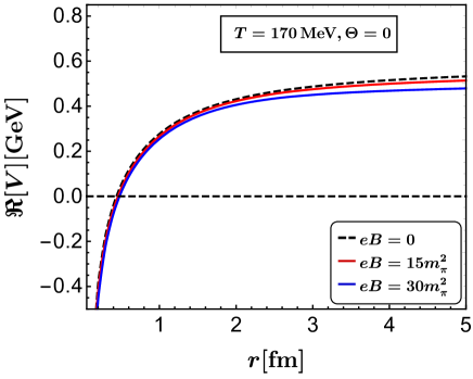
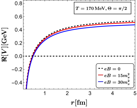
Figure 1: The real part of the potential is plotted as a function of quark-antiquark separation $r$ for $\Theta=0$ (left) and $\Theta=\pi/2$ (right) at $T=170$ MeV.

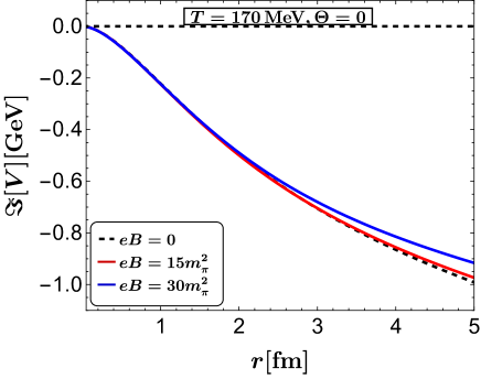
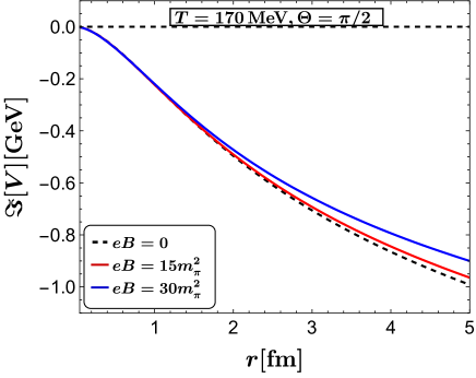
Figure 2: The imaginary part of the potential is plotted as a function of quark-antiquark separation $r$ for $\Theta=0$ (left) and $\Theta=\pi/2$ (right) at $T=170$ MeV.

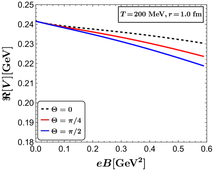
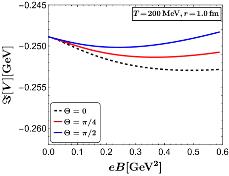
Figure 3: The complex potential is plotted as a function of the strength of the magnetic field for different values of $\Theta$ when $r=1$ fm and $T=200$ MeV. The left panel shows the variation of the real part of the potential. The right panel shows the variation of the imaginary part of the potential.

Here we take $\alpha=4/3\,\alpha_{s}(\Lambda^{2},B)$ and $\sigma=0.18$ GeV² and $\epsilon(p)$ is the dielectric permittivity, which is defined in Eq. (24). After substituting Eqs. (24) and (26) in Eq. (25), we obtain both the real as well as imaginary part of the potential, which contains both the perturbative Coulombic and nonperturbative string terms. The real part of the potential can be written in terms of Coulombic and string terms as

$$\Re V({\bm{r},T,B})=\Re V_{c}({\bm{r},T,B})+\Re V_{\sigma}({\bm{r},T,B}),$$ (27)

where the Coulombic term is

$$\Re V_{c}(\bm{r},T,B) = -\frac{\alpha}{2\pi^{2}}\int d^{3}{\bm{p}}$$ (28)

$$\times \Bigg{[}\frac{e^{i\boldsymbol{p\cdot r}}}{p^{2}+\Pi^{L}}-\frac{\Pi^{L}}{p^{2}(p^{2}+\Pi^{L})}\Bigg{]},~{}~{}~{}~{}~{}$$

and the string term reads

$$\Re V_{\sigma}(\bm{r},T,B)=-\frac{\sigma}{\pi^{2}}\int\!\!\frac{d^{3}{\bm{p}}}{(2\pi)^{3}}(e^{i{\bm{p}}\cdot{\bm{r}}}-1)\frac{1}{p^{2}(p^{2}+\Pi^{L})}.\hskip 18.49411pt$$ (29)

Here ${\bm{p}}\cdot{\bm{r}}=rp\big{[}\sin\theta\sin\Theta\cos(\phi-\Phi)+\cos\theta\cos\Theta\big{]}$ and the angles $\theta(\Theta)$ and $\phi(\Phi)$ are polar and azimuthal angles in momentum (coordinate) space, respectively. After integrating over the azimuthal angle, we obtain

$$\Re V({r,T,B,\Theta})=-\frac{1}{\pi}\int\frac{\sin\theta\,d\theta\,dp}{p^{2}+\Pi^{L}}\Big{[}(\alpha\,\Pi^{L}-2\,\sigma)$$

$$\times(\alpha\,p^{2}+2\,\sigma)e^{ipr\cos\theta\cos\Theta}J_{0}(p\hskip 0.85358ptr\hskip 0.85358pt\sin\theta\sin\Theta)\Big{]},$$ (30)

where $J_{0}$ is the Bessel’s function of the first kind.

Similarly, we compute the imaginary part of the quarkonium potential. The imaginary part of the potential is given by

$$\Im V({\bm{r},T,B})=T\int\frac{d^{3}{\bm{p}}}{2\pi}\frac{(e^{i\bm{p\cdot r}}-1)\Pi^{L}p}{\left(p^{2}+\Pi^{L}\right)^{2}}\left[\frac{\alpha}{p^{2}}+\frac{2\sigma}{p^{4}}\right].~{}~{}~{}~{}$$ (31)

After integrating over the azimuthal angle, we obtain

$$\Im V({r,\Theta,T,B})=-T\int\frac{\sin\theta\,d\theta\,dp}{\left(p^{2}+\Pi^{L}\right)^{2}}\Pi^{L}\left[\alpha\hskip 0.85358ptp+\frac{2\sigma}{p}\right]$$

$$\times\Big{\{}1-e^{ipr\cos\theta\cos\Theta}J_{0}(pr\sin\theta\sin\Theta)\Big{\}}.\,\,\,\,\,\,\,\,$$ (32)

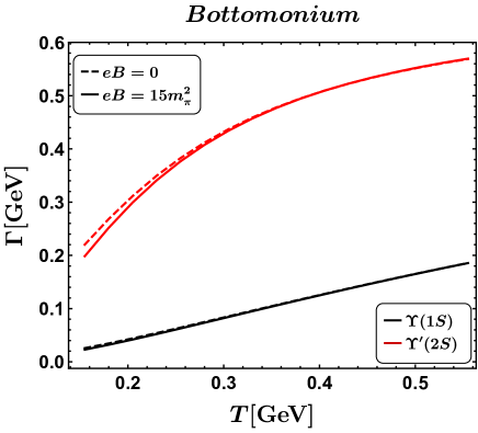
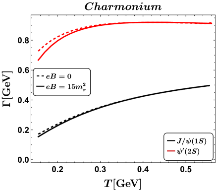
Figure 4: The thermal widths of bottomonium (left) and charmonium (right) states as a function of temperature at $B=0$ and $15m_{\pi}^{2}$ are shown.

We numerically solve the real (30) and imaginary (32) parts of the potential. In Fig. 1, we plot the real part of the potential as a function of separation distance $r$ for different strengths of the magnetic field $eB$. The left panel shows for the $Q\bar{Q}$ dipole axis alignment along the direction of the magnetic field ($\Theta=0$), whereas the right panel shows its perpendicular alignment with respect to the magnetic field ($\Theta=\pi/2$). We find that the real part of the potential becomes flattened with the magnetic field, due to an increase in screening with $B$. The effect of screening is seen to be slightly higher in the perpendicular case than along the direction of magnetic field.

In Fig. 2, we plot the imaginary part of the potential for $\Theta=0$ (left) and $\Theta=\pi/2$ (right) for the different values of the magnetic field. The imaginary part of the potential shows different behavior at smaller and larger $r$; it increases with the magnetic field at smaller $r$ and decreases in magnitude with the increase in the magnetic field at larger $r$. The decrease in magnitude with the magnetic field is observed to be higher for $\Theta=\pi/2$ compared to $\Theta=0$. Note that the magnetic field dependence is insignificant for the potential, especially in the range $eB=0$ to $eB=15m_{\pi}^{2}$.

Figure 3 shows the real and imaginary part of the potential as a function of magnetic field for different values of $\Theta$ at $r=1$ fm. We observe that the real part of the potential varies in response to a magnetic field at different rates according to direction. The magnetic field dependence is found to be maximum in $\Theta=\pi/2$ direction and minimum along the direction of the magnetic field, which establishes the anisotropy of the potential in the magnetic field. The magnitude of the imaginary part of the potential initially increases when the magnetic field increases, and diminishes as the magnetic field intensifies. Both components of the potential depend on both the magnitude of the magnetic field and the angle, however, this dependence is minimal.

The imaginary part increases in magnitude with the increase in the magnetic field initially, and the magnitude decreases as the magnetic field increases. Both the parts of the potential depend on the magnetic field and the angle between the dipole axis and the magnetic field, but the dependence is rather weak.

In the next section, we use the imaginary part of the potential to obtain the thermal widths of the quarkonium states.

IV Thermal Width

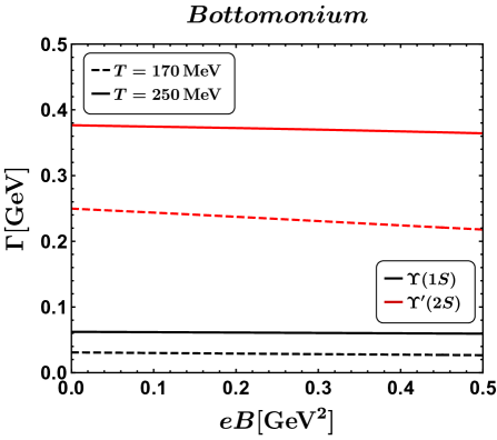
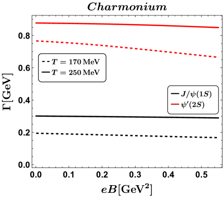
Figure 5: Thermal widths of bottomonium (left) and charmonium (right) states as a function of magnetic field for $T=170$ MeV and $250$ MeV.

In this section, we compute the thermal widths of the quarkonium states. The imaginary part of the potential estimates the thermal width, $\Gamma_{Q\bar{Q}}$, when treated as a perturbation of the vacuum potential. We compute the decay width of the quarkonium states as [3, 86]

$$\Gamma_{Q\bar{Q}}(T,B)=-\langle\psi(r)|\Im\,V_{Q\bar{Q}}(r,T,B,\Theta)|\psi(r)\rangle,$$ (33)

where $\psi(r)$ is the unperturbed Coulombic wave function. As the leading contribution to the imaginary potential for a deeply heavy-quark bound state is Coulombic, which justifies the use of Coulomb wave functions to calculate the thermal width. The wave function for the ground and excited states is given by

$$\psi_{1s}({r}) = \frac{1}{(\pi a_{0}^{3})^{1/2}}e^{-r/a_{0}},$$

$$\psi_{2s}({r}) = \frac{1}{4(2\pi a_{0}^{3})^{1/2}}\left(2-\frac{r}{a_{0}}\right)e^{-r/2a_{0}},$$ (34)

where $a_{0}=2/C_{F}m_{Q}\alpha_{s}$ is the Bohr radius of the $Q\bar{Q}$ system and $m_{Q}$ is the heavy quark mass. After substituting Eqs. (34) and (32) in Eq. (33), we obtain the thermal width of the quarkonium states for the ground state as

$$\Gamma_{1s}(T,B)=-\frac{1}{\pi a_{0}^{3}}\int d^{3}{\bf r}\,e^{-2r/a_{0}}\Im V\left(r,T,B,\Theta\right),\,$$ (35)

$$\Gamma_{1s}(T,B) \!\!=\!\! \frac{2T}{a_{0}^{3}}\int dr\,d\Theta\,r^{2}\sin\Theta e^{-2r/a_{0}}\int\frac{\sin\theta\,d\theta\,dp}{\left(p^{2}+\Pi^{L}\right)^{2}}\Pi^{L}\left[\alpha\hskip 0.85358ptp+\frac{2\sigma}{p}\right],\hskip 17.07182pt$$ (36)

and for the first excited states ($2S$) as

$$\Gamma_{2s}(T,B)=\frac{T}{16a_{0}^{3}}\int dr\,d\Theta\,r^{2}\sin\Theta\left(2-\frac{r}{a_{0}}\right)^{2}e^{-r/a_{0}}\int\frac{\sin\theta\,d\theta\,dp}{\left(p^{2}+\Pi^{L}\right)^{2}}\Pi^{L}\left[\alpha\hskip 0.85358ptp+\frac{2\sigma}{p}\right].\hskip 17.07182pt$$ (37)

We numerically compute the thermal widths of the ground (36) and excited (37) states of the bottomonium and charmonium states. In Fig. 4, we present plots of the thermal widths of the ground and first excited states of bottomonium (on the left) and charmonium (on the right) as a function of temperature for both $eB=0$ and $eB=15m_{\pi}^{2}$.

It is observed that the thermal width increases with an increase in temperature, as anticipated. The magnetic field effect is more on the first excited state than the ground state for both the bottomonium and charmonium states. At larger $r$, the effect of the magnetic field on the imaginary part of the potential is more due to the larger size of the excited states. Hence the excited states are more sensitive to the magnetic field than the ground state. Figure 5 shows the variation of thermal width with the magnetic field at different temperatures for bottomonium (left) and charmonium (right) states. We find that the thermal widths are more sensitive to the magnetic field at lower temperatures than the higher temperatures. The magnetic field effects decrease with the increase in heavy quark mass and decrease in the size of bound states. It can be concluded from the figures that the magnetic field has only a negligible effect on the thermal width compared to the temperature.

V Strong field approximation

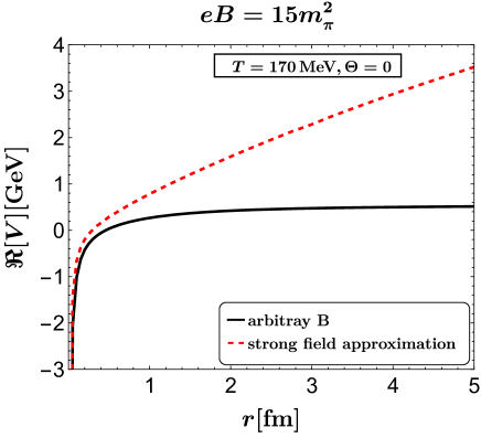
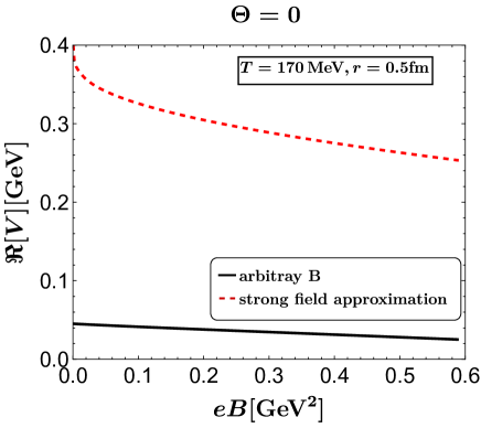
Figure 6: The real part of the potential as a function of $r$ is shown on the left side for an arbitrary (black solid) and strong magnetic field approximation (red dashed) at $T=170$ MeV and $\Theta=0$. The right side illustrates the same potential as a function of $eB$ at these conditions.

In this section, we compute the longitudinal component of the gluon self-energy in the strong magnetic field approximation ($T\ll\sqrt{|eB|}$). In the strong magnetic field limit ($|eB|\rightarrow\infty$), the fermion propagator [Eq. (4)] for massless case becomes

$$\widetilde{S}_{l}(\bf{k}) = -i\int_{0}^{\infty}ds\,e^{-s[\hat{\omega}_{l}^{2}+k_{3}^{2}+k^{2}_{\perp}/|q_{f}B|s]}$$ (38)

$$\times (-\hat{\omega}_{l}\gamma_{4}-k_{3}\gamma_{3})[1-i\gamma_{1}\gamma_{2}],$$

$$= ie^{-k^{2}_{\perp}/|q_{f}B|}\frac{\hat{\omega}_{l}\gamma_{4}+k_{3}\gamma_{3}}{\hat{\omega}_{l}^{2}+k_{3}^{2}}[1-i\gamma_{1}\gamma_{2}],$$

which is similar to the expression for the fermion propagator computed for the lowest Landau level approximation in Refs. [95, 31]. In $|eB|\rightarrow\infty$ limit, the temperature dependent part of the longitudinal component of the gluon self-energy (7) reduces to the dominant term as

$$\Pi_{q}^{L}({\omega_{n},\bf p},B) = -\sum_{f}\frac{g^{2}}{(4\pi)^{2}}\frac{(q_{f}B)^{2}}{T^{2}}e^{-p_{\perp}^{2}/2q_{f}B}\int_{0}^{\infty}\frac{du}{u^{2}}$$ (39)

$$\times \int_{-1}^{1}dv\,e^{-cu}\sum_{l\geq 1}(-1)^{(l+1)}l^{2}e^{-d/u}$$

$$\times \cos\pi ln(1-v),$$

where $c=(1-v^{2})(p_{3}^{2}+\omega_{n}^{2})/(4\,q_{f}B)$ and $d=l^{2}q_{f}B/4T^{2}$. The integration over $u$ can be done analytically using the relation

$$\int_{0}^{\infty}\frac{du}{u^{2}}e^{-cu-d/u}=2\sqrt{\frac{c}{d}}K_{1}(2\sqrt{c\,d}).$$ (40)

Here $K_{n}(z)$ represents the modified Bessel function of the second kind. Therefore, the longitudinal component of the gluon self-energy (39) for the strong magnetic field approximation in the static limit ($\omega_{n}\rightarrow 0$) becomes

$$\Pi_{q}^{L}({\bf p},B) = -\sum_{f}\frac{g^{2}q_{f}B}{8\pi^{2}T}e^{-p_{\perp}^{2}/2q_{f}B}\,\sum_{l\geq 1}(-1)^{(l+1)}$$ (41)

$$\times\int\limits_{-1}^{1}dv\,l\ p_{3}\sqrt{1-v^{2}}K_{1}\left(\frac{l\,p_{3}}{2T}\sqrt{1-v^{2}}\right).$$

Further, we compute the Debye screening mass from Eq. (7) in the limit $p\rightarrow 0$, for the regime where $T\ll\sqrt{eB}$

$$m_{D}^{2}(T,B) = -\lim_{{\bf p}\to 0}\Pi^{L}_{q}({\bf p},B),$$ (42)

$$= \sum_{f}\frac{g^{2}q_{f}B}{8\pi^{2}T^{2}}\int_{0}^{\infty}\frac{du}{u^{2}}\coth q_{f}B\,u\sum_{l\geq 1}(-1)^{l+1}l^{2}$$

$$\vspace{0.5cm}\ \times\ e^{-l^{2}/4uT^{2}},$$

$$= \sum_{f}\frac{g^{2}q_{f}B}{4\pi^{2}}.$$

In the absence of a magnetic field, the Debye screening mass becomes

$$m_{D}^{2}(T) = \frac{1}{3}C_{A}g^{2}T^{2}+\sum_{f}\frac{g^{2}}{8\pi^{2}T^{2}}\int_{0}^{\infty}\frac{du}{u^{3}}$$ (43)

$$\times\sum_{l\geq 1}(-1)^{l+1}l^{2}e^{-l^{2}/4uT^{2}},$$

$$= \frac{1}{3}C_{A}g^{2}T^{2}+\frac{1}{6}N_{f}g^{2}T^{2}.$$

The longitudinal component of gluon self-energy in strong field approximation obtained in Eq. (41) can be substituted in Eq. (25) to study the behavior of quarkonium potential in the strong field approximation. In Fig. 6, we show the effect of arbitrary magnetic fields and the strong field approximation on the real part of the potential. We find that the real part of the potential is more suppressed for the case of an arbitrary magnetic field as compared to strong field approximation due to larger screening in an arbitrary $B$. We can see that the potential with approximation differs in large values from the exact potential for any realistic magnetic field magnitude, and the difference gradually reduces as the magnetic field increases. Hence we can say that the strong field approximation is invalid, and one should consider the general case while studying the properties of quarkonium states.

VI Summary

In the present work, we have evaluated the influence of a magnetic field on the heavy quarkonium complex potential. We initially computed the dielectric permittivity from the static limit of the gluon propagator. This propagator was derived from the one-loop gluon self-energy in the presence of an external magnetic field, which was evaluated using Schwinger’s proper time formalism in Euclidean space. The effect of the magnetic field enters through the quark-loop contribution to the gluon self-energy and coupling constant. Then, we computed the in-medium heavy quarkonium complex potential using the modified dielectric permittivity. Results showed that this potential is anisotropic and varies with magnetic field strength and angle $\Theta$ between quark-antiquark axis and direction of magnetic field.

For very high magnetic field strengths, the real part of the potential gets flattened due to an increase in screening with $eB$. On the other hand, the imaginary part of the quarkonium potential experiences a rise in magnitude at short distances, followed by a decrease at long distances. Furthermore, the inclusion of a magnetic field introduces an angular dependence into the potential. Finally, we observed that the overall effect of the magnetic field on the complex potential is rather small for realistic strengths of magnetic field generated in heavy ion collisions.

We computed the decay widths of the ground and first excited states of bottomonium ($\Upsilon,\Upsilon^{\prime}$) and charmonium ($J/\psi,\psi^{\prime}$) using the imaginary part of the potential. We found that the excited states $(\Upsilon^{\prime},\psi^{\prime})$ are more sensitive to the magnetic field than the ground states $(\Upsilon,J/\psi)$. The effect of magnetic fields decreases with increasing heavy quark mass and decreasing size, making the charmonium states more sensitive to magnetic field strength than the bottomonium states. For the decay widths, as the temperature increases, the sensitivity to magnetic fields decreases, eventually disappearing at high temperatures.

We have further compared our results with the strong-field approximated potential. We found that such an approximated potential does not even come close to the potential without such an approximation for any realistic magnetic field value generated in heavy ion collisions. The approximation makes the screening much weaker as compared to an estimation for the arbitrary magnetic field. The strong magnetic field approximated screening however gradually increases as the magnetic field increases. The present investigation invalidates the strong magnetic field approximation usually adopted in literature for the heavy quarkonium complex potential. For the realistic strengths of magnetic fields, one needs to take the effects of a general magnetic field as has been attempted here. Moreover, it may also be noted that, the weak-field expansion introduces new divergences in the gluon propagators, and one needs a way to regulate it. Hence, it is essential to study the effect of arbitrary magnetic fields on the heavy quarkonium complex potential and the properties of quarkonium states.

In the future, we would like to extend our computation for the moving medium in the presence of an arbitrary magnetic field.

VII Acknowledgments

J. S.  would like to thank R. Ghosh for the useful discussions. L. T.  is supported by the Korean Ministry of Education, Science and Technology, Gyeongsangbuk-do and Pohang City at the APCTP and National Research Foundation (NRF) funded by the Ministry of Science of Korea (Grant No. 2021R1F1A1061387). N.H. is supported in part by the SERB-MATRICS under Grant No. MTR/2021/000939.

References

- [1] T. Matsui and H. Satz, “ Suppression by Quark-Gluon Plasma Formation,” Phys. Lett. B 178 (1986) 416–422.
- [2] L. Thakur, N. Haque, U. Kakade, and B. K. Patra, “Dissociation of quarkonium in an anisotropic hot QCD medium,” Phys. Rev. D88 no. 5, (2013) 054022, arXiv:1212.2803 [hep-ph].
- [3] L. Thakur, U. Kakade, and B. K. Patra, “Dissociation of Quarkonium in a Complex Potential,” Phys. Rev. D89 no. 9, (2014) 094020, arXiv:1401.0172 [hep-ph].
- [4] M. Y. Jamal, I. Nilima, V. Chandra, and V. K. Agotiya, “Dissociation of heavy quarkonia in an anisotropic hot QCD medium in a quasiparticle model,” Phys. Rev. D97 no. 9, (2018) 094033, arXiv:1805.04763 [nucl-th].
- [5] V. K. Agotiya, V. Chandra, M. Y. Jamal, and I. Nilima, “Dissociation of heavy quarkonium in hot QCD medium in a quasiparticle model,” Phys. Rev. D 94 no. 9, (2016) 094006, arXiv:1610.03170 [nucl-th].
- [6] Q. Du, A. Dumitru, Y. Guo, and M. Strickland, “Bulk viscous corrections to screening and damping in QCD at high temperatures,” JHEP 01 (2017) 123, arXiv:1611.08379 [hep-ph].
- [7] L. Thakur, N. Haque, and Y. Hirono, “Heavy quarkonia in a bulk viscous medium,” JHEP 06 (2020) 071, arXiv:2004.03426 [hep-ph].
- [8] L. Thakur and Y. Hirono, “Spectral functions of heavy quarkonia in a bulk-viscous quark gluon plasma,” JHEP 02 (2022) 207, arXiv:2111.08225 [hep-ph].
- [9] A. Islam, L. Dong, Y. Guo, A. Rothkopf, and M. Strickland, “The effective complex heavy-quark potential in an anisotropic quark-gluon plasma,” EPJ Web Conf. 274 (2022) 04015, arXiv:2210.12102 [hep-ph].
- [10] L. Dong, Y. Guo, A. Islam, A. Rothkopf, and M. Strickland, “The complex heavy-quark potential in an anisotropic quark-gluon plasma — Statics and dynamics,” JHEP 09 (2022) 200, arXiv:2205.10349 [hep-ph].
- [11] M. Kurian, M. Singh, V. Chandra, S. Jeon and C. Gale, “Charm quark dynamics in quark-gluon plasma with 3 + 1D viscous hydrodynamics,” Phys. Rev. C102 no. 4, (2020) 044907, arXiv:2007.07705 [hep-ph].
- [12] M. Singh, M. Kurian, S. Jeon and C. Gale, “Open charm phenomenology with a multi-stage approach to relativistic heavy-ion collisions,” arXiv:2306.09514 [nucl-th].
- [13] L. Thakur, N. Haque, and H. Mishra, “Heavy quarkonium moving in hot and dense deconfined nuclear matter,” Phys. Rev. D95 no. 3, (2017) 036014, arXiv:1611.04568 [hep-ph].
- [14] M. A. Escobedo, J. Soto, and M. Mannarelli, “Non-relativistic bound states in a moving thermal bath,” Phys. Rev. D 84 (2011) 016008, arXiv:1105.1249 [hep-ph].
- [15] M. A. Escobedo, F. Giannuzzi, M. Mannarelli, and J. Soto, “Heavy Quarkonium moving in a Quark-Gluon Plasma,” Phys. Rev. D 87 no. 11, (2013) 114005, arXiv:1304.4087 [hep-ph].
- [16] J. Sebastian, M. Y. Jamal, and N. Haque, “Liénard-Wiechert potential of a heavy quarkonium moving in QGP medium,” Phys. Rev. D 107 no. 5, (2023) 054040, arXiv:2207.08510 [hep-ph].
- [17] S. Chakraborty and N. Haque, “Holographic quark-antiquark potential in hot, anisotropic Yang-Mills plasma,” Nucl. Phys. B 874 821-851, (2013), arXiv:1212.2769 [hep-th].
- [18] B. K. Patra, H. Khanchandani, and L. Thakur, “Velocity-induced Heavy Quarkonium Dissociation using the gauge-gravity correspondence,” Phys. Rev. D92 no. 8, (2015) 085034, arXiv:1504.05396 [hep-th].
- [19] ALICE Collaboration, J. Adam et al., “Measurement of an excess in the yield of at very low in Pb-Pb collisions at = 2.76 TeV,” Phys. Rev. Lett. 116 no. 22, (2016) 222301, arXiv:1509.08802 [nucl-ex].
- [20] K. Marasinghe and K. Tuchin, “Quarkonium dissociation in quark-gluon plasma via ionization in magnetic field,” Phys. Rev. C 84 (2011) 044908, arXiv:1103.1329 [hep-ph].
- [21] J. Alford and M. Strickland, “Charmonia and Bottomonia in a Magnetic Field,” Phys. Rev. D 88 (2013) 105017, arXiv:1309.3003 [hep-ph].
- [22] C. S. Machado, F. S. Navarra, E. G. de Oliveira, J. Noronha, and M. Strickland, “Heavy quarkonium production in a strong magnetic field,” Phys. Rev. D 88 (2013) 034009, arXiv:1305.3308 [hep-ph].
- [23] S. Cho, K. Hattori, S. H. Lee, K. Morita, and S. Ozaki, “QCD sum rules for magnetically induced mixing between and ,” Phys. Rev. Lett. 113 no. 17, (2014) 172301, arXiv:1406.4586 [hep-ph].
- [24] X. Guo, S. Shi, N. Xu, Z. Xu, and P. Zhuang, “Magnetic Field Effect on Charmonium Production in High Energy Nuclear Collisions,” Phys. Lett. B 751 (2015) 215–219, arXiv:1502.04407 [hep-ph].
- [25] T. Yoshida and K. Suzuki, “Heavy meson spectroscopy under strong magnetic field,” Phys. Rev. D 94 (2016) 074043, arXiv:1607.04935 [hep-ph].
- [26] A. V. Sadofyev and Y. Yin, “The charmonium dissociation in an “anomalous wind”,” JHEP 01 (2016) 052, arXiv:1510.06760 [hep-th].
- [27] C. Bonati, M. D’Elia, M. Mariti, M. Mesiti, F. Negro, A. Rucci, and F. Sanfilippo, “Screening masses in strong external magnetic fields,” Phys. Rev. D 95 no. 7, (2017) 074515, arXiv:1703.00842 [hep-lat].
- [28] C. Bonati, M. D’Elia, and A. Rucci, “Heavy quarkonia in strong magnetic fields,” Phys. Rev. D 92 no. 5, (2015) 054014, arXiv:1506.07890 [hep-ph].
- [29] R. Rougemont, R. Critelli, and J. Noronha, “Anisotropic heavy quark potential in strongly-coupled SYM in a magnetic field,” Phys. Rev. D 91 no. 6, (2015) 066001, arXiv:1409.0556 [hep-th].
- [30] D. Dudal and T. G. Mertens, “Melting of charmonium in a magnetic field from an effective AdS/QCD model,” Phys. Rev. D 91 (2015) 086002, arXiv:1410.3297 [hep-th].
- [31] B. Karmakar, A. Bandyopadhyay, N. Haque, and M. G. Mustafa, “General structure of gauge boson propagator and its spectra in a hot magnetized medium,” Eur. Phys. J. C 79 no. 8, (2019) 658, arXiv:1804.11336 [hep-ph].
- [32] A. Bandyopadhyay, B. Karmakar, N. Haque, and M. G. Mustafa, “Pressure of a weakly magnetized hot and dense deconfined QCD matter in one-loop hard-thermal-loop perturbation theory,” Phys. Rev. D 100 no. 3, (2019) 034031, arXiv:1702.02875 [hep-ph].
- [33] M. Y. Jamal, J. Prakash, I. Nilima and A. Bandyopadhyay, “Energy loss of heavy quarks in the presence of magnetic field,” arXiv:2304.09851 [hep-ph].
- [34] B. Karmakar, R. Ghosh and A. Mukherjee, “Collective modes of gluons in an anisotropic thermomagnetic medium,” Phys. Rev. D 106 no. 11, (2022) 116006, arXiv:2204.09646 [hep-ph].
- [35] K. K. Gowthama, M. Kurian and V. Chandra, “Response of a weakly magnetized hot QCD medium to an inhomogeneous electric field,” Phys. Rev. D 103 no. 7, (2021) 074017, arXiv:2012.07156 [hep-ph].
- [36] D. E. Kharzeev, L. D. McLerran, and H. J. Warringa, “The Effects of topological charge change in heavy ion collisions: ’Event by event P and CP violation’,” Nucl. Phys. A 803 (2008) 227–253, arXiv:0711.0950 [hep-ph].
- [37] K. Tuchin, “Particle production in strong electromagnetic fields in relativistic heavy-ion collisions,” Adv. High Energy Phys. 2013 (2013) 490495, arXiv:1301.0099 [hep-ph].
- [38] V. Skokov, A. Y. Illarionov, and V. Toneev, “Estimate of the magnetic field strength in heavy-ion collisions,” Int. J. Mod. Phys. A 24 (2009) 5925–5932, arXiv:0907.1396 [nucl-th].
- [39] W.-T. Deng and X.-G. Huang, “Event-by-event generation of electromagnetic fields in heavy-ion collisions,” Phys. Rev. C 85 (2012) 044907, arXiv:1201.5108 [nucl-th].
- [40] A. Bzdak and V. Skokov, “Event-by-event fluctuations of magnetic and electric fields in heavy ion collisions,” Phys. Lett. B 710 (2012) 171–174, arXiv:1111.1949 [hep-ph].
- [41] I. A. Shovkovy, “Magnetic Catalysis: A Review,” Lect. Notes Phys. 871 (2013) 13–49, arXiv:1207.5081 [hep-ph].
- [42] F. Bruckmann, G. Endrodi, and T. G. Kovacs, “Inverse magnetic catalysis and the Polyakov loop,” JHEP 04 (2013) 112, arXiv:1303.3972 [hep-lat].
- [43] B. Chatterjee, H. Mishra and A. Mishra, “ Vacuum structure and chiral symmetry breaking in strong magnetic fields for hot and dense quark matter,” Phys. Rev. D 84 (2011) 014016, arXiv:1101.0498 [hep-ph].
- [44] G. S. Bali, F. Bruckmann, G. Endrodi, F. Gruber, and A. Schaefer, “Magnetic field-induced gluonic (inverse) catalysis and pressure (an)isotropy in QCD,” JHEP 04 (2013) 130, arXiv:1303.1328 [hep-lat].
- [45] V. Voronyuk, V. D. Toneev, W. Cassing, E. L. Bratkovskaya, V. P. Konchakovski, and S. A. Voloshin, “(Electro-)Magnetic field evolution in relativistic heavy-ion collisions,” Phys. Rev. C 83 (2011) 054911, arXiv:1103.4239 [nucl-th].
- [46] K. Fukushima, D. E. Kharzeev, and H. J. Warringa, “The Chiral Magnetic Effect,” Phys. Rev. D 78 (2008) 074033, arXiv:0808.3382 [hep-ph].
- [47] B. Alver and G. Roland, “Collision geometry fluctuations and triangular flow in heavy-ion collisions,” Phys. Rev. C 81 (2010) 054905, arXiv:1003.0194 [nucl-th]. [Erratum: Phys.Rev.C 82, 039903 (2010)].
- [48] M. Kurian, S. Mitra, S. Ghosh and V. Chandra, “Transport coefficients of hot magnetized QCD matter beyond the lowest Landau level approximation,” Eur. Phys. J. C 79 no. 2, (2019) 134, arXiv:1805.07313 [nucl-th].
- [49] R. Ghosh, B. Karmakar and M. Golam Mustafa, “Chiral susceptibility in a dense thermomagnetic QCD medium within the hard thermal loop approximation,” Phys. Rev. D 103 (2021) 074019, arXiv:2103.08407 [hep-ph].
- [50] STAR Collaboration, J. Adam et al., “First Observation of the Directed Flow of and in Au+Au Collisions at = 200 GeV,” Phys. Rev. Lett. 123 no. 16, (2019) 162301, arXiv:1905.02052 [nucl-ex].
- [51] S. K. Das, S. Plumari, S. Chatterjee, J. Alam, F. Scardina, and V. Greco, “Directed Flow of Charm Quarks as a Witness of the Initial Strong Magnetic Field in Ultra-Relativistic Heavy Ion Collisions,” Phys. Lett. B 768 (2017) 260–264, arXiv:1608.02231 [nucl-th].
- [52] ALICE Collaboration, S. Acharya et al., “Probing the effects of strong electromagnetic fields with charge-dependent directed flow in Pb-Pb collisions at the LHC,” Phys. Rev. Lett. 125 no. 2, (2020) 022301, arXiv:1910.14406 [nucl-ex].
- [53] B. Singh, L. Thakur, and H. Mishra, “Heavy quark complex potential in a strongly magnetized hot QGP medium,” Phys. Rev. D 97 no. 9, (2018) 096011, arXiv:1711.03071 [hep-ph].
- [54] R. Ghosh, A. Bandyopadhyay, I. Nilima, and S. Ghosh, “Anisotropic tomography of heavy quark dissociation by using the general propagator structure in a finite magnetic field,” Phys. Rev. D 106 no. 5, (2022) 054010, arXiv:2204.02312 [hep-ph].
- [55] M. Hasan, B. Chatterjee, and B. K. Patra, “Heavy Quark Potential in a static and strong homogeneous magnetic field,” Eur. Phys. J. C 77 no. 11, (2017) 767, arXiv:1703.10508 [hep-ph].
- [56] M. Hasan and B. K. Patra, “Dissociation of heavy quarkonia in a weak magnetic field,” Phys. Rev. D 102 no. 3, (2020) 036020, arXiv:2004.12857 [hep-ph].
- [57] H.-X. Zhang, “Responses of quark-antiquark interaction and heavy quark dynamics to magnetic field,” arXiv:2301.09110 [hep-ph].
- [58] G. Huang, J. Zhao, and P. Zhuang, “Quantum color screening in external magnetic field,” arXiv:2208.01407 [hep-ph].
- [59] J. Zhao, K. Zhou, S. Chen, and P. Zhuang, “Heavy flavors under extreme conditions in high energy nuclear collisions,” Prog. Part. Nucl. Phys. 114 (2020) 103801, arXiv:2005.08277 [nucl-th].
- [60] A. Mishra and S. P. Misra, “Masses and decay widths of charmonium states in the presence of strong magnetic fields,” Phys. Rev. C 102 no. 4, (2020) 045204, arXiv:2004.01007 [nucl-th].
- [61] Y. Chen, X.-L. Sheng, and G.-L. Ma, “Electromagnetic fields from the extended Kharzeev-McLerran-Warringa model in relativistic heavy-ion collisions,” Nucl. Phys. A 1011 (2021) 122199, arXiv:2101.09845 [nucl-th].
- [62] S. Iwasaki, M. Oka, and K. Suzuki, “A review of quarkonia under strong magnetic fields,” Eur. Phys. J. A 57 no. 7, (2021) 222, arXiv:2104.13990 [hep-ph].
- [63] K. Fukushima, K. Hattori, H.-U. Yee, and Y. Yin, “Heavy Quark Diffusion in Strong Magnetic Fields at Weak Coupling and Implications for Elliptic Flow,” Phys. Rev. D 93 no. 7, (2016) 074028, arXiv:1512.03689 [hep-ph].
- [64] M. Kurian, V. Chandra, and S. K. Das, “Impact of longitudinal bulk viscous effects to heavy quark transport in a strongly magnetized hot QCD medium,” Phys. Rev. D 101 no. 9, (2020) 094024, arXiv:2002.03325 [nucl-th].
- [65] M. Kurian, S. K. Das, and V. Chandra, “Heavy quark dynamics in a hot magnetized QCD medium,” Phys. Rev. D 100 no. 7, (2019) 074003, arXiv:1907.09556 [nucl-th].
- [66] I. Nilima, A. Bandyopadhyay, R. Ghosh and S. Ghosh, “Heavy quark potential and LQCD based quark condensate at finite magnetic field,” Eur. Phys. J. C 83 no. 1, 30 (2023), arXiv:2204.02388 [hep-ph].
- [67] M. Debnath, R. Ghosh and N. Haque, “The complex heavy-quark potential with the Gribov-Zwanziger action,” arXiv:2305.16250 [hep-ph].
- [68] W. Lucha, F. F. Schoberl, and D. Gromes, “Bound states of quarks,” Phys. Rept. 200 (1991) 127–240.
- [69] N. Brambilla, A. Pineda, J. Soto, and A. Vairo, “Effective Field Theories for Heavy Quarkonium,” Rev. Mod. Phys. 77 (2005) 1423, arXiv:hep-ph/0410047 [hep-ph].
- [70] F. Karsch, M. T. Mehr, and H. Satz, “Color Screening and Deconfinement for Bound States of Heavy Quarks,” Z. Phys. C37 (1988) 617.
- [71] P. K. Srivastava, O. S. K. Chaturvedi, and L. Thakur, “Heavy quarkonia in a potential model: binding energy, decay width, and survival probability,” Eur. Phys. J. C 78 no. 6, (2018) 440, arXiv:1806.09348 [nucl-th].
- [72] E. Eichten, K. Gottfried, T. Kinoshita, J. B. Kogut, K. D. Lane, and T.-M. Yan, “The Spectrum of Charmonium,” Phys. Rev. Lett. 34 (1975) 369–372. [Erratum: Phys. Rev. Lett.36,1276(1976)].
- [73] E. Eichten, K. Gottfried, T. Kinoshita, K. D. Lane, and T.-M. Yan, “Charmonium: Comparison with Experiment,” Phys. Rev. D 21 (1980) 203.
- [74] M. Laine, O. Philipsen, P. Romatschke, and M. Tassler, “Real-time static potential in hot QCD,” JHEP 03 (2007) 054, arXiv:hep-ph/0611300 [hep-ph].
- [75] M. Laine, O. Philipsen, and M. Tassler, “Thermal imaginary part of a real-time static potential from classical lattice gauge theory simulations,” JHEP 09 (2007) 066, arXiv:0707.2458 [hep-lat].
- [76] Y. Burnier, M. Laine, and M. Vepsalainen, “Heavy quarkonium in any channel in resummed hot QCD,” JHEP 01 (2008) 043, arXiv:0711.1743 [hep-ph].
- [77] A. Beraudo, J. P. Blaizot, and C. Ratti, “Real and imaginary-time Q anti-Q correlators in a thermal medium,” Nucl. Phys. A806 (2008) 312–338, arXiv:0712.4394 [nucl-th].
- [78] N. Brambilla, J. Ghiglieri, A. Vairo, and P. Petreczky, “Static quark-antiquark pairs at finite temperature,” Phys. Rev. D 78 (2008) 014017, arXiv:0804.0993 [hep-ph].
- [79] N. Brambilla, M. A. Escobedo, J. Ghiglieri, and A. Vairo, “Thermal width and gluo-dissociation of quarkonium in pNRQCD,” JHEP 12 (2011) 116, arXiv:1109.5826 [hep-ph].
- [80] N. Brambilla, M. A. Escobedo, J. Ghiglieri, and A. Vairo, “Thermal width and quarkonium dissociation by inelastic parton scattering,” JHEP 05 (2013) 130, arXiv:1303.6097 [hep-ph].
- [81] M. Margotta, K. McCarty, C. McGahan, M. Strickland, and D. Yager-Elorriaga, “Quarkonium states in a complex-valued potential,” Phys. Rev. D83 (2011) 105019, arXiv:1101.4651 [hep-ph]. [Erratum: Phys. Rev.D84,069902(2011)].
- [82] A. Rothkopf, T. Hatsuda, and S. Sasaki, “Complex Heavy-Quark Potential at Finite Temperature from Lattice QCD,” Phys. Rev. Lett. 108 (2012) 162001, arXiv:1108.1579 [hep-lat].
- [83] Y. Burnier and A. Rothkopf, “Disentangling the timescales behind the non-perturbative heavy quark potential,” Phys. Rev. D86 (2012) 051503, arXiv:1208.1899 [hep-ph].
- [84] Y. Burnier and A. Rothkopf, “A gauge invariant Debye mass and the complex heavy-quark potential,” Phys. Lett. B753 (2016) 232–236, arXiv:1506.08684 [hep-ph].
- [85] A. Rothkopf, “Heavy Quarkonium in Extreme Conditions,” Phys. Rept. 858 (2020) 1–117, arXiv:1912.02253 [hep-ph].
- [86] A. Dumitru, Y. Guo, and M. Strickland, “The Imaginary part of the static gluon propagator in an anisotropic (viscous) QCD plasma,” Phys. Rev. D79 (2009) 114003, arXiv:0903.4703 [hep-ph].
- [87] P. Petreczky, C. Miao, and A. Mocsy, “Quarkonium spectral functions with complex potential,” Nucl. Phys. A855 (2011) 125–132, arXiv:1012.4433 [hep-ph].
- [88] C. Bonati, S. Calì, M. D’Elia, M. Mesiti, F. Negro, A. Rucci, and F. Sanfilippo, “Effects of a strong magnetic field on the QCD flux tube,” Phys. Rev. D 98 no. 5, (2018) 054501, arXiv:1807.01673 [hep-lat].
- [89] C. Bonati, M. D’Elia, M. Mariti, M. Mesiti, F. Negro, A. Rucci, and F. Sanfilippo, “Magnetic field effects on the static quark potential at zero and finite temperature,” Phys. Rev. D 94 no. 9, (2016) 094007, arXiv:1607.08160 [hep-lat].
- [90] V. Agotiya, V. Chandra, and B. K. Patra, “Dissociation of quarkonium in hot QCD medium: Modification of the inter-quark potential,” Phys. Rev. C80 (2009) 025210, arXiv:0808.2699 [hep-ph].
- [91] J. Alexandre, “Vacuum polarization in thermal QED with an external magnetic field,” Phys. Rev. D 63 (2001) 073010, arXiv:hep-th/0009204.
- [92] J. S. Schwinger, “On gauge invariance and vacuum polarization,” Phys. Rev. 82 (1951) 664–679.
- [93] A. Ayala, C. A. Dominguez, S. Hernandez-Ortiz, L. A. Hernandez, M. Loewe, D. Manreza Paret, and R. Zamora, “Thermomagnetic evolution of the QCD strong coupling,” Phys. Rev. D 98 no. 3, (2018) 031501(R), arXiv:1805.08198 [hep-ph].
- [94] H. A. Weldon, “Reformulation of finite temperature dilepton production,” Phys. Rev. D 42 (1990) 2384–2387.
- [95] V. P. Gusynin, V. A. Miransky, and I. A. Shovkovy, “Dimensional reduction and catalysis of dynamical symmetry breaking by a magnetic field,” Nucl. Phys. B 462 (1996) 249–290, arXiv:hep-ph/9509320.