ExoMol line lists – LIII: Empirical Rovibronic spectra of Yttrium Oxide (YO)

Abstract

Empirical line lists BRYTS for the open shell molecule ⁸⁹Y¹⁶O (yttrium oxide) and its isotopologues are presented. The line lists cover the 6 lowest electronic states: $X\,{}^{2}\Sigma^{+}$, $A\,{}^{2}\Pi$, $A^{\prime}\,{}^{2}\Delta$, $B\,{}^{2}\Sigma^{+}$, $C\,{}^{2}\Pi$ and $D\,{}^{2}\Sigma^{+}$ up to 60 000 cm^-1 ($<0.167$ $\mu$m) for rotational excitation up to $J=400.5$. An ab initio spectroscopic model consisting of potential energy curves (PECs), spin-orbit and electronic angular momentum couplings is refined by fitting to experimentally determined energies of YO, derived from published YO experimental transition frequency data. The model is complemented by empirical spin-rotation and $\Lambda$-doubling curves and ab initio dipole moment and transition dipole moment curves computed using MRCI. The ab initio PECs computed using the complete basis set limit extrapolation and the CCSD(T) method with its higher quality provide an excellent initial approximation for the refinement. Non-adiabatic coupling curves for two pairs of states of the same symmetry $A$/$C$ and $B$/$D$ are computed using a state-averaged CASSCF and used to build diabatic representations for the $A\,{}^{2}\Pi$, $C\,{}^{2}\Pi$, $B\,{}^{2}\Sigma^{+}$ and $D\,{}^{2}\Sigma^{+}$ curves. The experimentally derived energies of ⁸⁹Y¹⁶O utilised in the fit are used to replace the corresponding calculated energy values in the BRYTS line list. Simulated spectra of YO show excellent agreement with the experiment, where it is available. Calculated lifetimes of YO are tuned to agree well with the experiment, where available. The BRYTS YO line lists are available from the ExoMol database (www.exomol.com).

1 Introduction

The spectrum of yttrium oxide, YO, has been the subject of many astrophysical studies. It has been observed in the spectra of cool stars (Wyckoff & Clegg, 1978) including R-Cygni (Sauval, 1978; Murty, 1982), Pi-Gruis (Murty, 1983), V838 Mon (Goranskii & Barsukova, 2007; Kaminski et al., 2009), and V4332 Sgr (Goranskii & Barsukova, 2007; Tylenda et al., 2015). YO has also been actively used in laser cooling experiments (Yeo et al., 2015; Collopy et al., 2015; Quéméner & Bohn, 2016; Collopy et al., 2018). Its spectrum has been used as a probe to study high-temperature materials (Badie et al., 2005a).

There are many laboratory spectroscopic studies of YO, including its $A\,{}^{2}\Pi$ – $X\,{}^{2}\Sigma^{+}$ (Shin & Nicholls, 1977; Linton, 1978; Bernard et al., 1979; Liu & Parson, 1979; Wijchers et al., 1980; Bagare & Murthy, 1982; Bernard & Gravina, 1983; Wijchers et al., 1984; Childs et al., 1988; Steimle & Shirley, 1990; Dye et al., 1991; Fried et al., 1993; Otis & Goodwin, 1993; Badie & Granier, 2002, 2003; Badie et al., 2005a, b; Kobayashi & Sekine, 2006; Badie et al., 2007a; Badie et al., 2007b; Collopy et al., 2015; Mukund & Nakhate, 2023), $B\,{}^{2}\Sigma^{+}$ – $X\,{}^{2}\Sigma^{+}$ (Shin & Nicholls, 1977; Bernard et al., 1979; Bernard & Gravina, 1980; Fried et al., 1993; Leung et al., 2005; Zhang et al., 2017), $A^{\prime}\,{}^{2}\Delta$ – $X\,{}^{2}\Sigma^{+}$(Chalek & Gole, 1976; Simard et al., 1992; Collopy et al., 2015) and $D\,{}^{2}\Sigma^{+}$ – $X\,{}^{2}\Sigma^{+}$ (Zhang et al., 2017) band systems, rotational spectrum (Uhler & Akerlind, 1961; Steimle & Alramadin, 1986; Hoeft & Torring, 1993), hyperfine spectrum (Kasai & Weltner, 1965; Steimle & Alramadin, 1986, 1987; Childs et al., 1988; Suenram et al., 1990; Knight et al., 1999; Steimle & Virgo, 2003) and chemiluminescence spectra (Manos & Parson, 1975; Chalek & Gole, 1977; Fried et al., 1993). The very recent experimental study of the $A\,{}^{2}\Pi$ and $B\,{}^{2}\Sigma^{+}$ systems of YO by Mukund & Nakhate (2023) provided crucial information for this work on the coupling between the $B\,{}^{2}\Sigma^{+}$ and $D\,{}^{2}\Sigma^{+}$ states. Relative intensity measurements of the $A\,{}^{2}\Pi$ – $X\,{}^{2}\Sigma^{+}$ system were performed by Bagare & Murthy (1982). Permanent dipole moments of YO in both the $X\,{}^{2}\Sigma^{+}$ and $A\,{}^{2}\Pi$ states have been measured using the Stark technique (Steimle & Shirley, 1990; Suenram et al., 1990; Steimle & Virgo, 2003). The lifetimes in the $A\,{}^{2}\Pi$, $B\,{}^{2}\Sigma^{+}$, and $D\,{}^{2}\Sigma^{+}$ states were measured by Liu & Parson (1977) and Zhang et al. (2017).

Our high-level ab initio study (Smirnov et al., 2019) forms a prerequisite for this work, where a mixture of multireference configuration interaction (MRCI) and coupled cluster methods were used to produce potential energy cures (PECs), spin–orbit curves (SOCs), electronic angular momentum curves (EAMCs), electric dipole moment curves (DMCs), and transition dipole moment curves (TDMCs) covering the six lowest electronic states of YO. Other theoretical studies of YO include MRCI calculations by Langhoff & Bauschlicher (1988) and CASPT2 calculations of spectroscopic constants by Zhang et al. (2017).

In this paper, the ab initio spectroscopic model of Smirnov et al. (2019) is extended by introducing non-adiabatic coupling curves for two pairs of states, $A$/$C$ and $B$/$D$, and then refined by fitting to experimentally derived energies of YO using our coupled nuclear-motion program Duo (Yurchenko et al., 2016). The energies are constructed using a combination of the spectroscopic constants and line positions taken from the literature through a procedure based on the MARVEL (Furtenbacher et al., 2007) methodology. The new empirical spectroscopic model is used to produce the hot line list BRYTS for three major isotopologues of YO, ⁸⁹Y¹⁶O, ⁸⁹Y¹⁷O and ⁸⁹Y¹⁸O as part of the ExoMol project (Tennyson & Yurchenko, 2012; Tennyson et al., 2020).

2 Experimental information

Although the spectroscopy of YO has been extensively studied, some key high resolution experimental sources from the 1970-80s only provide spectroscopic constants rather than original transition frequencies; this limits their usability for high resolution applications. For cases where only spectroscopic constants are available we used an effective Hamiltonian model to compute the corresponding energy term values. This includes term values for the ground electronic $X\,{}^{2}\Sigma^{+}$ state. In the following, experimental studies of YO are reviewed.

61UhAk: Uhler & Akerlind (1961) reported line positions from the $B\,{}^{2}\Sigma^{+}$–$X\,{}^{2}\Sigma^{+}$ (0,0) and $A\,{}^{2}\Pi$–$X\,{}^{2}\Sigma^{+}$ (0,0) bands, but the $B\,{}^{2}\Sigma^{+}$–$X\,{}^{2}\Sigma^{+}$ band is fully covered by more recent and accurate data (Bernard & Gravina, 1980). The quantum numbers $F_{1}$ and $F_{2}$ of $B\,{}^{2}\Sigma^{+}$–$X\,{}^{2}\Sigma^{+}$  had to be swapped to agree with Bernard & Gravina (1980). However, due to many conflicting combination differences, only high $J$ transitions ($J>100.5$) were included in our final analysis.

77ShNi: Shin & Nicholls (1977) performed an analysis of the blue-green $B\,{}^{2}\Sigma^{+}$–$X\,{}^{2}\Sigma^{+}$ and orange $A\,{}^{2}\Pi$–$X\,{}^{2}\Sigma^{+}$ systems but no rovibronic assignment was reported and their data are not used here.

79BeBaLu: Bernard et al. (1979) reported an extensive analysis of the $A$–$X$ ($v^{\prime}=0,1,2,3,4,5$) and $B$–$X$ ($v^{\prime}=0,1$) systems. Only spectroscopic constants were reported. This work has been superseded by more recent studies and therefore is not used here.

80BeGr: Bernard & Gravina (1980) reported line positions from the $B\,{}^{2}\Sigma^{+}$–$X\,{}^{2}\Sigma^{+}$ system, $v^{\prime}=0,1$ and $v^{\prime\prime}=0,1,2,3$ and spectroscopic constants for $v^{\prime}=0,1,2,3$, in emission in a hollow cathode discharge with a partial analysis of the $(3,2)$ and $(4,3)$ bands (only higher $J\geq 35.5$ and $J\geq 57.5$, respectively). The data were included in our analysis.

83BeGr: Bernard & Gravina (1983) presented a study of the $A\,{}^{2}\Pi$-$X\,{}^{2}\Sigma^{+}$ system of YO excited in the discharge of a hollow cathode tube. Only spectroscopic constants were reported, covering the $X\,{}^{2}\Sigma^{+}$ ($v=0\ldots 10$) and $A\,{}^{2}\Pi$ ($v=0\ldots 9$) vibronic states ($v=6$ and $v=7$ with a limited analysis). We used these constants and the effective Hamiltonian of Bacis et al. (1977) to generate term values for the states $v=0\ldots 5$, 8 and 9 ($A\,{}^{2}\Pi$). It should be noted that the spectroscopic program Pgopher Western (2017) could not be used as its ${}^{2}\Pi$ model is found to be incompatible with that used by Bernard & Gravina (1983) despite constants sharing the same names. A simple Python code based on the effective Hamiltonian expressions of Bacis et al. (1977) is provided as part of our supplementary material. Band heads of $v^{\prime}=7-15$ ($\Omega=0.5$) and $v^{\prime}=6,8,9$ ($\Omega=1.5$) were reported, but not used directly in the fit here. It is known that effective Hamiltonian expansions can diverge at high $J$, we therefore limited the corresponding energies to about $J\leq 100.5$.

The coverage of the spectroscopic constants of $X\,{}^{2}\Sigma^{+}$ is up to $v=10$, while the available line positions are only up to $v=3$, which is why we opted to use the spectroscopic constants by Bernard & Gravina (1983) to generate the $X\,{}^{2}\Sigma^{+}$ term values. YO has a relatively rigid structure in its ground electronic state potential with the vibronic energies well separated from each other and other electronic state.

92SiJaHa: Simard et al. (1992) reported line positions from the $A^{\prime}\,{}^{2}\Delta$–$X\,{}^{2}\Sigma^{+}$ system (0,0) in their laser-induced fluorescence spectral study with a pulsed dye laser. It was included in the analysis here.

93HoTo: Hoeft & Torring (1993) reported a microwave spectrum of $X\,{}^{2}\Sigma^{+}$ for $v=0,1,2,3$. It was included in the analysis here.

05LeMaCh: Leung et al. (2005) reported a cavity ring-down absorption spectrum of the $B\,{}^{2}\Sigma^{+}$–$X\,{}^{2}\Sigma^{+}$  (2,0) and (2,1) system. We included their line positions in the analysis here.

15CoHuYe: Collopy et al. (2015) reported three THz lines from the $A\,{}^{2}\Pi$–$X\,{}^{2}\Sigma^{+}$ $(0,0)$ system with low uncertainties recorded for laser cooling application. These were included in our analysis.

17ZhZhZh: Zhang et al. (2017) reported line positions from the $D\,{}^{2}\Sigma^{+}$–$X\,{}^{2}\Sigma^{+}$ system (0,0) and (1,0) which were used in the analysis here.

23MuNa: Mukund & Nakhate (2023) reported a high-resolution analysis of the highly excited $A\,{}^{2}\Pi$–$X\,{}^{2}\Sigma^{+}$ ($v^{\prime}=11,12,13$) and $B\,{}^{2}\Sigma^{+}$–$X\,{}^{2}\Sigma^{+}$  ($v^{\prime}=5,6$) systems. For the $A$–$X$ band, only the $\Omega=0.5$ branch was provided. Their line positions were included in our analysis. There is a crossing between $A\,{}^{2}\Pi$, $v=11$ and $D\,{}^{2}\Sigma^{+}$, $v=2$ around $J=34.5$, see Fig. 1.

The only experimental information on the transition probabilities available for YO includes the permanent dipole moments in the $X\,{}^{2}\Sigma^{+}$ and $A\,{}^{2}\Pi$ states measured by Steimle & Shirley (1990); Suenram et al. (1990); Steimle & Virgo (2003) and the lifetimes of some lower lying vibrational states measured by Liu & Parson (1977) ($A\,{}^{2}\Pi$) and Zhang et al. (2017) ($B\,{}^{2}\Sigma^{+}$ and $D\,{}^{2}\Sigma^{+}$).

3 Description of the pseudo-MARVEL procedures

MARVEL (Measured Active Rotational Vibrational Energy Levels) is a spectroscopic network algorithm (Furtenbacher et al., 2007), now routinely used for constructing ExoMol line lists for high-resolution applications (Tennyson et al., 2020). We did not have sufficient original experimental line positions for a proper MARVEL analysis of the YO spectroscopic data, which were mostly only available represented by spectroscopic constants. Furthermore, there are no studies of the infrared spectrum of YO which meant that the (lower) ground energies could be only reconstructed from lower quality UV transitions, which limits the quality of the MARVEL energies.

Instead, a ‘pseudo-MARVEL’ procedure was applied as follows (see also Yurchenko et al. (2022)). The experimental frequencies $\tilde{\nu}_{ij}$, where available, were utilised to generate rovibronic energies of YO as upper states energies using

$$\tilde{E}_{j(i)}^{\rm(upp)}=\tilde{E}^{\rm(low)}_{i}+\tilde{\nu}_{ij},$$ (1)

which were then averaged over all transitions connecting the same upper state $j$. All experimental transitions originate from or end up at the $X\,{}^{2}\Sigma^{+}$  state. We used the spectroscopic constants from Bernard & Gravina (1983) ($v=0,1,\ldots,10$) to generate the $X\,{}^{2}\Sigma^{+}$ state energies $\tilde{E}^{\rm(low)}_{i}$ in conjunction with the program Pgopher. The $A\,{}^{2}\Pi$ state energies were generated using the effective Hamiltonian (Bacis et al., 1977) except for $v=0$, $J>100.5$, which were obtained using the pseudo-MARVEL procedure. This pseudo-MARVEL analysis yielded 5089 empirically determined energy levels which we used in the fit. The final experimentally determined energy set covers the following vibronic bands $X$: $v=0-10$; $A^{\prime}$: $v=0$, $J_{\rm max}=14.5$; $A$: $v=$ 0,1,2,3,4,5, 8,9, 11,12,13; $B$: $v=0,1,2,3,4,5,6$; $D$: $v=0,1$. The vibrational and rotational coverage is illustrated in Fig. 2. The experimental transition frequencies collected as part of this work are provided in the Supporting Information to this paper in the MARVEL format together with the pseudo-MARVEL energies used in the fit.

It should be noted that the effective Hamiltonians used do not provide any information on direct perturbations between vibronic bands caused by their crossing or any other inter-band interactions. For example, the $A\,{}^{2}\Pi$ $v=5$ and $B\,{}^{2}\Sigma^{+}$ $v=0$ states cross at around $J=27.5$. We excluded energy values in the vicinity of such crossings from the fit. The only crossing represented by the real data is between the $D\,{}^{2}\Sigma^{+}$ $v=2$ and $A\,{}^{2}\Pi$ $v=11$ bands (Mukund & Nakhate, 2023), see Fig. 1.

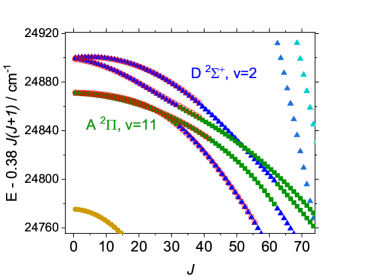
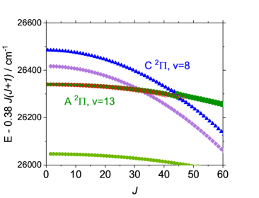
Figure 1: Illustration of the crossings: $D\,{}^{2}\Sigma^{+}$, $v=2$ and $A\,{}^{2}\Pi$, $v=11$ bands (left) and $A\,{}^{2}\Pi$, $v=13$ and $C\,{}^{2}\Pi$, $v=8$ (right), with experimental values shown as empty circle.

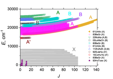
Figure 2: Experimentally derived energy term values of YO used in the refinement of the ab initio spectroscopic model.

4 Ab initio calculations

Non-adiabatic couplings (NACs) or the first-order derivative couplings between the state pairs $X\,{}^{2}\Sigma^{+}-B\,{}^{2}\Sigma^{+}$, $X\,{}^{2}\Sigma^{+}-D\,{}^{2}\Sigma^{+}$, $B\,{}^{2}\Sigma^{+}-D\,{}^{2}\Sigma^{+}$ and $A\,{}^{2}\Pi-C\,{}^{2}\Pi$  were derived by three-point central differences for CASSCF wavefunctions using the DDR procedure as implemented in MOLPRO (Werner et al., 2020). The state-averaged CASSCF method was employed with density matrix averaging over six low-lying doublet states (three $\Sigma^{+}$, two $\Pi$, and one $\Delta$) with equal weights for each of the roots. The active space included 7 electrons distributed in 13 orbitals (6$a_{1}$, 3$b_{1}$, 3$b_{2}$, 1$a_{2}$) that had predominantly oxygen 2p and yttrium 4d, 5s, 5p, and 6s character; all lower energy orbitals were constrained to be doubly occupied. Augmented triple-zeta quality basis sets aug-cc-pwCVTZ (Peterson & Dunning, 2002) on O and pseudopotential-based aug-cc-pwCVTZ-PP (Peterson et al., 2007) on Y were used in these calculations. The resulting NACs are illustrated in Fig. 3.

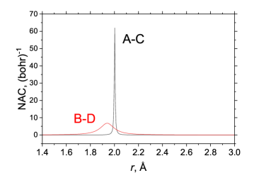
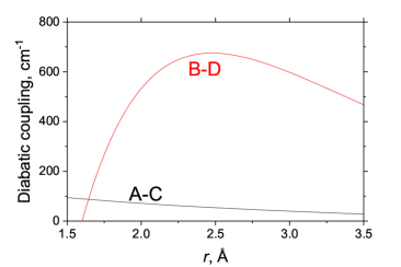
Figure 3: CASSCF NACs and empirical diabatic couplings $D(r)$ of YO, A–C and B–D.

5 Spectroscopic model

Our starting point is the ab initio spectroscopic model of YO developed by Smirnov et al. (2019), which includes PECs, SOCs, TDMCs, EAMCs for six lowest doublet states of YO in the adiabatic representation. YO exhibits non-adiabatic effects via the couplings of the two pairs of states: $A\,{}^{2}\Pi$ with $C\,{}^{2}\Pi$ and $B\,{}^{2}\Sigma^{+}$ with $D\,{}^{2}\Sigma^{+}$. Apart from the avoided crossing in these PECs, other adiabatic curves (SOCs, EAMCs, (T)DMCs) also have strongly distorted shapes exhibiting step-like behaviour, which makes the adiabatic representation far from ideal for refinement. This is not only because these curves are difficult to represent analytically as parameterised functions of the bond length (required for the fit), but also because the shapes of the curves around any avoided crossing are very sensitive to the precise position of these crossings, which are also difficult to control in the adiabatic representation. Due to these effects, SOCs, EAMCs and (T)DMCs between the $B\,{}^{2}\Sigma^{+}$, $D\,{}^{2}\Sigma^{+}$ and the $A\,{}^{2}\Pi$, $C\,{}^{2}\Pi$ states also exhibit discontinuous behaviour in the region of the avoided crossing, which can only be correctly treated in combination with the NAC curves as well as their second-order derivative couplings (which we did not compute). Vibronic intensities, for instance, are very sensitive to the description of the steep structures in the adiabatic DMCs. Because of inaccuracies in the ab initio calculations, the adiabatic DMCs will be prone to large errors in their shape since the strong, steep gradient variations around the avoided crossing are sensitive to both crossing position and morphology, and so will negatively affect the corresponding spectral properties. These sharp behaviours are difficult to model, so the diabatic representation is a natural choice since DMCs and other couplings will become smooth, and less sensitive to inaccuracies in ab initio calculations.

We therefore decided to work in the diabatic representation taking advantage of the recent developments in Duo (Brady et al., 2022; Brady et al., 2023). To this end, a diabatic spectroscopic model of YO was generated by diabatising the ab initio adiabatic PECs, SOCs, EAMCs and (T)DMCs of YO (Smirnov et al., 2019) as outlined in the following.

Unfortunately, the ab initio adiabatic curves reported in Smirnov et al. (2019) were not suitable for a direct diabatisation using the corresponding NACs due to incomplete ab initio curves and inconsistent levels of theory used for different properties. Effectively, only the PECs of the six electronic states of YO computed using the complete basis set limit (CBS) extrapolation from awCVQZ and awCV5Z in conjunction with the CCSD(T) method were suitable for accurate descriptions of the corresponding crossings in the diabatic representations. All other property curves (SOCs, EAMCs, (T)DMCs) were computed with MRCI or even CASSCF and did not provide adequate coverage, especially at longer bond lengths ($r>1.9$ Å) beyond the avoided crossing points (see Figs. 9 and 10 in Smirnov et al. (2019)).

In order to overcome this problem, in line with the property-based diabatisation (see, e.g. 22ShVaZo), we constructed diabatic curves under the assumption that in the diabatic representations all the curves become smooth, without characteristic step-like shapes and manually constructed diabatic SOCs, EMACs, TDMCs. The existing points were inter- and extrapolated to best represent smooth diabatic curves. Admittedly, there is some arbitrariness in this approach which is subsequently resolved, at least partially, by empirically refining the initial curves. The various curves representing our diabatic spectroscopic model of YO are illustrated in Figs. 4–6.

5.1 Diabatisation

To represent the diabatic potential energy curves of the $X\,{}^{2}\Sigma^{+}$, $A\,{}^{2}\Pi$, $A^{\prime}\,{}^{2}\Delta$, $B\,{}^{2}\Sigma^{+}$, $C\,{}^{2}\Pi$ and $D\,{}^{2}\Sigma^{+}$ states analytically, we used the extended Morse oscillator (EMO) (Lee et al., 1999) function as well as the Extended Hulburt-Hirschfelder (EHH) function (Hulburt & Hirschfelder, 1941) as implemented in Duo. An EMO function is given by

$$V(r)=V_{\rm e}\;\;+\;\;(A_{\rm e}-V_{\rm e})\left[1\;\;-\;\;\exp\left(-\sum_{k=0}^{N}B_{k}\xi_{p}^{k}(r-r_{\rm e})\right)\right]^{2},$$ (2)

where $A_{\rm e}$ is a dissociation asymptote, $A_{\rm e}-V_{\rm e}$ is the dissociation energy, $r_{\rm e}$ is an equilibrium distance of the PEC, and $\xi_{p}$ is the Šurkus variable given by:

$$\xi_{p}=\frac{r^{p}-r^{p}_{\rm e}}{r^{p}+r^{p}_{\rm e}}.$$ (3)

The EMO form is our typical choice for representing PECs and was used here for the $X\,{}^{2}\Sigma^{+}$, $A\,{}^{2}\Pi$, $B\,{}^{2}\Sigma^{+}$ and $D\,{}^{2}\Sigma^{+}$ states. For the $A^{\prime}\,{}^{2}\Delta$ and $C\,{}^{2}\Pi$ states, which do not have much experimental information for refinement, we employ the EHH function. This form was suggested to be more suitable for the description of the dissociation region (Cazzoli et al., 2006). Here we use the EHH form from Ushakov et al. (2023) as given by

$$V_{\textrm{EHH}}(r)=D_{\textrm{e}}\left[\left(1-e^{-q}\right)^{2}+cq^{3}\left(1+\sum_{i=1}^{3}b_{i}q^{i}\right)e^{-2q}\right],$$ (4)

where $q=\alpha\left(r-r_{\textrm{e}}\right)$.

The corresponding parameters defining PECs were first obtained by fitting to the ab initio CCSD(T)/CBS potential energies and then empirically refined by fitting to empirical energies of YO (where available) as described below; these parameters are given in the supplementary material in the form of a Duo input file. The asymptotic energies $A_{\rm e}$ for all states but $B\,{}^{2}\Sigma^{+}$ were fixed to the value 59220 cm^-1, or 7.34 eV, which corresponds to $D_{0}$ = 7.290(87) eV determined by Ackermann & Rauh (1974), based on their mass spectrometric measurements. For the $B\,{}^{2}\Sigma^{+}$ state, $A_{\rm e}$ was fixed to a higher value of 75000 cm^-1 in order to achieve a physically sensible shape of the PEC. Otherwise, the $B\,{}^{2}\Sigma^{+}$ curve tended to cross the $D\,{}^{2}\Sigma^{+}$ curve also at $r\sim 4$ Å.

In principle, the property-based diabatisation does not require the usage of the NAC curves. However, in order to assist our diabatisations of the YO ab initio curves, we used the ab initio CASSCF NACs of $A$–$C$ and $B$-$D$ shown in Fig. 3 as a guide. These curves were fitted using the following Lorentzian functions:

$$\phi_{ij}(r)=\frac{1}{2}\frac{\gamma}{\gamma^{2}+(r-r_{\rm c})^{2}},$$ (5)

where $\gamma$ is the corresponding half-width-at-half-maximum (HWHM), while $r_{\rm c}$ is its centre, corresponding to the crossing point of diabatic curves.

The diabatic and adiabatic representations are connected via a unitary $2\times 2$ transformation given by

$${\bf U}(\beta(r))=\begin{bmatrix}\cos(\beta(r))&-\sin(\beta(r))\\ \sin(\beta(r))&\cos(\beta(r))\end{bmatrix},$$ (6)

where the $r$-dependent mixing angle $\beta(r)$ is obtained via the integral

$$\beta(r)=\int^{r}_{-\infty}\phi_{12}(r^{\prime})dr^{\prime}.$$ (7)

For the Lorentzian-type NAC in Eq. (5), the angle $\beta$ is given by

$$\beta=\frac{1}{2}\arctan\left(\frac{r-r_{\rm c}}{\gamma}\right)+\frac{\pi}{4}.$$ (8)

The diabatic representation is defined by two PECs $V_{1}(r)$ and $V_{2}(r)$ coupled with a diabatic term $D(r)$ as a $2\times 2$ diabatic matrix

$$\bf{A}=\left(\begin{array}[]{cc}V_{1}(r)&D(r)\\ D(r)&V_{2}(r)\end{array}\right).$$ (9)

The two eigenvalues of the matrix $\bf{A}$ provide the adiabatic PECs in the form of solution of a quadratic equation as given by

$$V_{\rm low}(r) = \frac{V_{1}(r)+V_{2}(r)}{2}-\frac{\sqrt{[V_{1}(r)-V_{2}(r)]^{2}+4\,D^{2}(r)}}{2},$$ (10)

$$V_{\rm upp}(r) = \frac{V_{1}(r)+V_{2}(r)}{2}+\frac{\sqrt{[V_{1}(r)-V_{2}(r)]^{2}+4\,D^{2}(r)}}{2},$$ (11)

where $V_{\rm low}(r)$ and $V_{\rm upp}(r)$ are the two adiabatic PECs.

Assuming the diabatic PECs $V_{1}(r)$ and $V_{2}(r)$ as well as NAC $\phi_{12}(r)$ are known, the diabatic coupling function $D(r)$ can be re-constructed using the condition that the non-diagonal coupling should vanish upon the unitary transformation $U(r)$ in Eq. (6) such that the adiabatic potential matrix is diagonal and is then given by:

$$D(r)=\frac{1}{2}\tan(2\beta(r))\left(V_{2}(r)-V_{1}(r)\right).$$ (12)

Assuming also the EMO functions for the PECs $V_{1}(r)$ and $V_{2}(r)$ as in Eq. (2) and the ‘Lorentzian’-type angle $\beta(r)$ in Eq. (8), the diabatic coupling curves for YO have an asymmetric Gaussian-like shape, see the right panel of Fig. 3; this is not always the case as the $V_{2}-V_{1}$ term in Eq. (12) heavily influences the morphology of $D(r)$.

For the $B\,{}^{2}\Sigma^{+}$–$D\,{}^{2}\Sigma^{+}$ pair, where the experimental data is better represented, in order to introduce some flexibility into the fit, we decided to model the diabatic coupling by directly representing it using an inverted EMO function from Eq. (2). This gives the asymmetric Gaussian-like shape, with the asymptote $A_{\rm e}$ set to zero and $V_{\rm e}$ representing the maximum of the diabatic coupling $D(r)$. The $A$–$C$ diabatic coupling was modelled using Eq. (12) with the two parameter ‘Lorentzian’-type angle $\beta(r)$ from Eq. (8).

5.2 Other coupling curves

For the SOC and EAMC curves of YO we used the expansion:

$$F(r)=\sum^{N}_{k=0}B_{k}\,z^{k}(1-\xi_{p})+\xi_{p}\,B_{\infty},$$ (13)

where $z$ is either taken as the Šurkus variable $z=\xi_{p}$ or a damped-coordinate given by:

$$z=(r-r_{\rm ref})\,e^{-\beta_{2}(r-r_{\rm ref})^{2}-\beta_{4}(r-r_{\rm ref})^{4}},$$ (14)

see also Prajapat et al. (2017) and Yurchenko et al. (2018a). Here $r_{\rm ref}$ is a reference position equal to $r_{\rm e}$ by default and $\beta_{2}$ and $\beta_{4}$ are damping factors. For the $X\,{}^{2}\Sigma^{+}$ state, a BOB (Born-Oppenheimer Breakdown) correction curve modelled using Eq. (13) was used. These parameterised representations were then used to refine the ab initio curves by fitting them to the experimentally derived rovibronic energies of YO. The final coupling curves are shown in Figs. 3 (right display), 4 and 5.

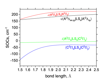
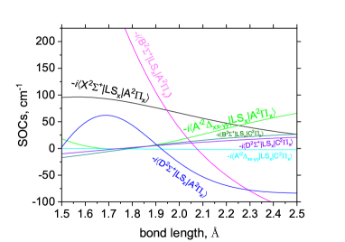
Figure 4: Refined SOCs of YO in the diabatic representation: diagonal and non-diagonal.

We also included spin-rotation and $\Lambda$-doubling $p(r)+2o(r)$ (Brown & Merer, 1979) curves as empirical objects for some of the electronic states modelled using Eq. (13), see Fig. 5.

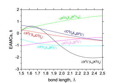
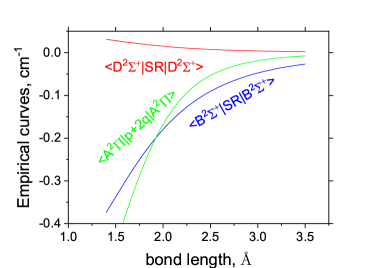
Figure 5: Refined EAMCs of YO in the diabatic representation, empirical spin-rotation corrections and $\Lambda$-doubling curves.

5.3 Dipoles

We diabatise our DMCs using a combination of cubic-spline interpolation to smooth out the region around the avoided crossing and knowledge of the shape of the diabatised target curves. Figure 7 illustrates our property-based diabatising ‘transformation’ for the $\langle B\,{}^{2}\Sigma^{+}|\mu_{z}|X\,{}^{2}\Sigma^{+}\rangle$ and $\langle D\,{}^{2}\Sigma^{+}|\mu_{z}|X\,{}^{2}\Sigma^{+}\rangle$ transition dipole moment pairs, the effect being the two curves ‘swap’ beyond the avoided crossing and are now smooth. Figure 6 shows all diabatised ab initio diagonal and off-diagonal DMCs, which are smooth over all bond lengths.

Within nuclear motion and intensity calculations dipoles are sometimes represented as a grid of ab initio points, however, one sees a flattening of the ground state IR overtone bands with vibrational excitation. The source of this nonphysical flattening has been discussed by Medvedev et al. (2015, 2016); Medvedev & Ushakov (2022); Ushakov et al. (2023). It comes from numerical noise in the calculations, which is enhanced by the interpolation of the given Molpro dipole grid points onto the Duo defined grid. The most effective method to reduce this numerical noise is to represent the input dipole moments analytically (Medvedev et al., 2015). We chose to represent our $X\,{}^{2}\Sigma^{+}$ DMC using the ‘irregular DMC’ proposed by Medvedev & Ushakov (2022) which takes the form

$$\mu_{\rm irreg}(r)=\chi(r;c_{2},...,c_{6})\sum_{i=0}^{6}b_{i}T_{i}(z(r))$$ (15)

where $T_{i}$ are Chebyshev polynomials of the first kind, $b_{i}$ are summation coefficients to be fitted, $z(r)$ is a reduced variable in bond length and is given by

$$z(r)=1-2e^{-c_{1}r}$$ (16)

which maps the $r\in[0,\infty]$ Å interval to the $z\in[-1,1]$ reduced interval (the region in which the Chebyshev polynomials have zeros), and finally $\chi(r;c_{2},...,c_{6})$ is an $r$-dependent term parametrically dependent on 5 $c_{k}$ parameters to be fitted and is given by

$$\chi(r;c_{2},...,c_{6})\frac{(1-e^{-c_{2}r})^{3}}{\sqrt{(r^{2}-c_{3}^{2})^{2}+c_{4}^{2}}\sqrt{(r^{2}-c_{5}^{2})^{2}+c_{6}^{2}}}.$$

The irregular DMC form has the desirable properties of quickly converging to the correct long-range limit, having enough parameters (13) to ensure minimal local oscillations, and provide a straight Normal Intensity Distribution Law (NIDL) (Medvedev & Ushakov, 2022; Medvedev, 2012; Medvedev et al., 2015). This straight NIDL is a major restriction to the model DMC and means the logarithm of the overtone vibrational transition dipole moments (VTDM) $\langle v^{\prime}|\mu(r)|v=0\rangle$ ($v^{\prime}>1$) should evolve linearly with the square root of the upper state energy over the harmonic frequency, or $\sqrt{v^{\prime}+\frac{1}{2}}$. Here we compute VTDMs $\langle v^{\prime}|\mu(r)|v=0\rangle$ up to dissociation for the $X\,{}^{2}\Sigma^{+}$ using both the grid-defined dipole and the fitted analytical form, where figure 8 shows their behaviour. The expected linear behaviour of the NIDL is shown in Fig. 8 as a gray line which is seen to better agree with the TDM computed using the analytical $X\,{}^{2}\Sigma^{+}$ DMC compared to the calculation using the grid-interpolated DMC. At the $v^{\prime}=6$ overtone the grid-interpolated DMC causes a non-physical flattening of the VTDM at $\sim 3.4\times 10^{-5}$ Debye, whereas we only see a departure from the straight NIDL at $v^{\prime}=15$ when using the analytical form which flattens at $\sim 7.4\times 10^{-10}$ Debye. The analytically represented $X\,{}^{2}\Sigma^{+}$ DMC therefore provides a more physically meaningful behaviour of the vibrational overtone VTDM but still departs from the expected NIDL at high overtones where the intensities are much lower and therefore less important.

Following Smirnov et al. (2019), we scaled the ab initio DMC of $X\,{}^{2}\Sigma^{+}$  by the factor 1.025 to match the experimental value of the equilibrium dipole $\langle X|,v=0|\mu(r)||X,v=0\rangle$ determined by Suenram et al. (1990). The DMCs of $A^{\prime}\,{}^{2}\Delta$, $A\,{}^{2}\Pi$ and $B\,{}^{2}\Sigma^{+}$ were scaled by 0.97, 0.86 and 0.6, respectively to match the more accurate CCSD(T)/CBS single point calculations from Smirnov et al. (2019).

The $A\,{}^{2}\Pi$–$X\,{}^{2}\Sigma^{+}$, $B\,{}^{2}\Sigma^{+}$–$X\,{}^{2}\Sigma^{+}$ and $D\,{}^{2}\Sigma^{+}$–$X\,{}^{2}\Sigma^{+}$ TDMCs had to be scaled by 0.8, 0.75 and 2.8, respectively, to improve the agreement of the corresponding calculated values of the $A\,{}^{2}\Pi$, $B\,{}^{2}\Sigma^{+}$ and $D\,{}^{2}\Sigma^{+}$ lifetimes with the measurements of Liu & Parson (1977) and Zhang et al. (2017), see discussion below.

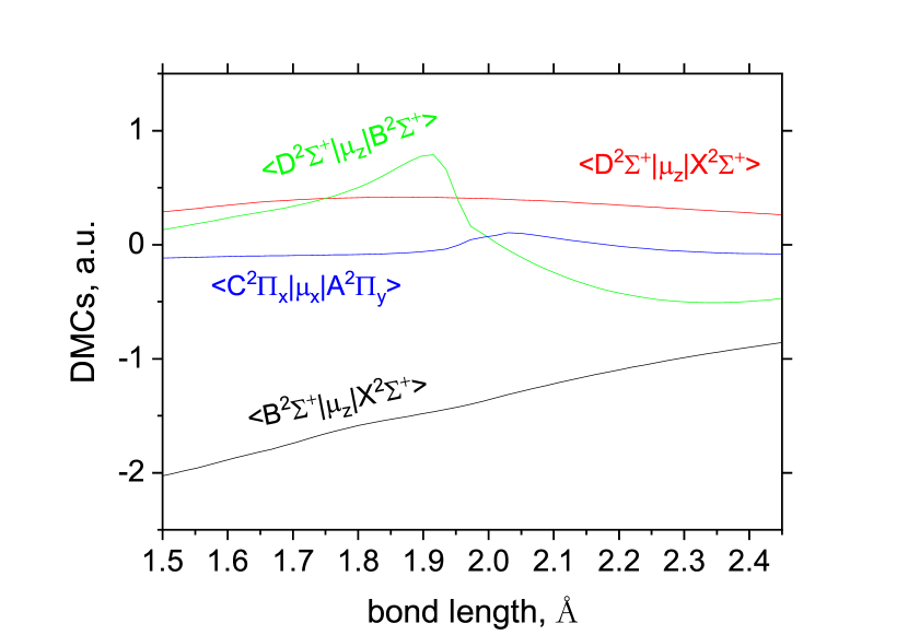
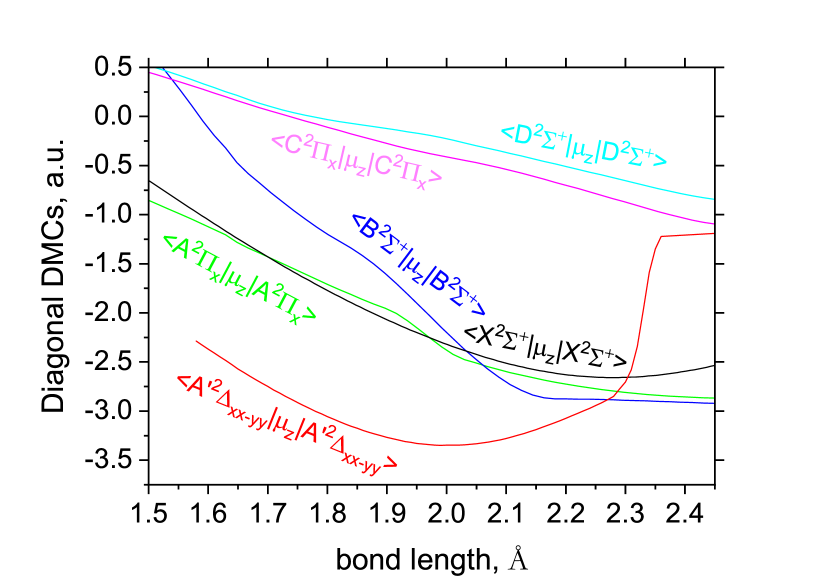
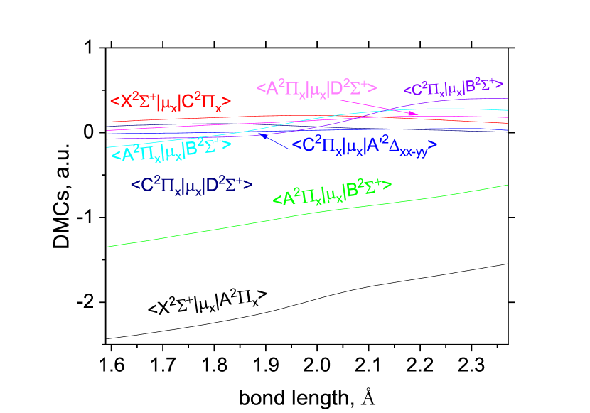
Figure 6: Diabatised ab initio dipole moment matrix elements (in a.u.) as a function of bond length. The middle panel gives diagonal dipoles while the top and bottom panels give transition dipole moments.

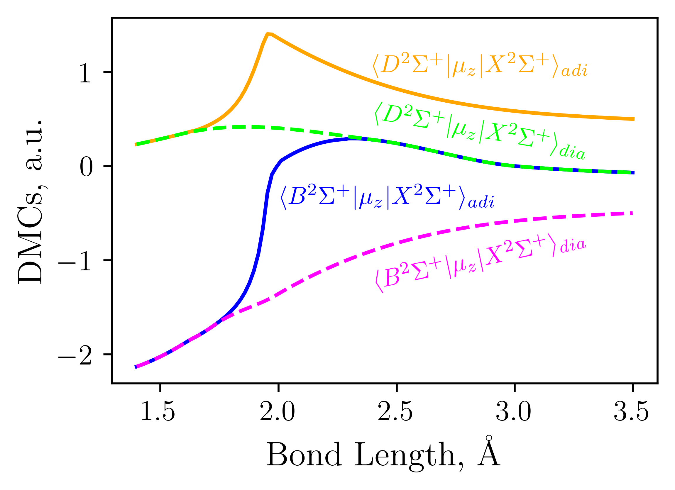
Figure 7: Example of the diabatisation (see text for details) of the adiabatic $\langle B\,{}^{2}\Sigma^{+}|\mu_{z}|X\,{}^{2}\Sigma^{+}\rangle$ and $\langle D\,{}^{2}\Sigma^{+}|\mu_{z}|X\,{}^{2}\Sigma^{+}\rangle$ dipole moment pairs, where the $B\,{}^{2}\Sigma^{+}$ and $D\,{}^{2}\Sigma^{+}$ states exhibit an avoided crossing at $r\sim 1.81$ Å.

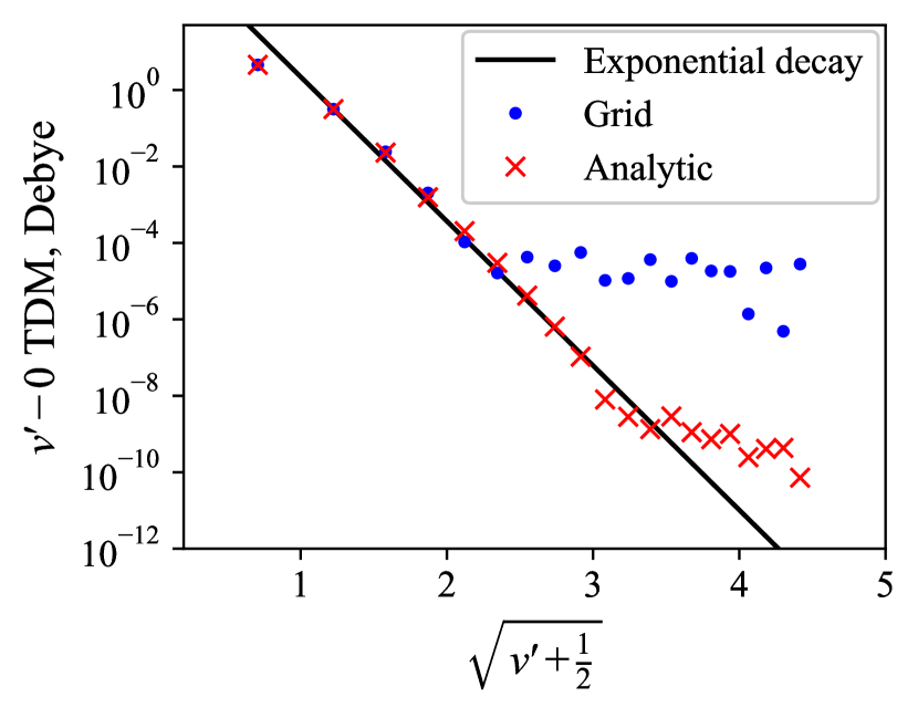
Figure 8: $X\,{}^{2}\Sigma^{+}$ $\rightarrow$ $X\,{}^{2}\Sigma^{+}$ $v^{\prime}-0$ overtone TDMs are plotted on a log scale vs. $\sqrt{v^{\prime}+\frac{1}{2}}$ and are computed using the grid interpolated ab initio DMC (shown as blue circles) and our fitted analytical model DMC (Eq. (15), shown as red crosses). A simple exponential decay is shown for comparison which simulates the expected NIDL-like behaviour (Medvedev, 2012).

6 Refinement of the spectroscopic model

We use the diatomic code Duo (Yurchenko et al., 2016) to solve a coupled system of Schrödinger equations. Duo is a free-access rovibronic solver for diatomic molecules available at https://github.com/exomol/Duo/. The hyperfine structure was ignored. For nuclear motion calculations a vibrational sinc-DVR basis set was defined as a grid of 151 internuclear geometries in the range of 1.4–3.5 Å. We select the lowest 30, 30, 35, 30, 30, 30 vibrational wavefunctions of the $X\,{}^{2}\Sigma^{+}$, $A^{\prime}\,{}^{2}\Delta$, $A\,{}^{2}\Pi$, $B\,{}^{2}\Sigma^{+}$, $C\,{}^{2}\Pi$, and $D\,{}^{2}\Sigma^{+}$ states, respectively, to form the contracted vibronic basis. A refined spectroscopic model of YO was obtained by fitting the expansion parameters representing different properties to 5089 empirically derived rovibrational energy term values of ⁸⁹Y¹⁶O described above.

The refined (diabatic) PECs of YO are illustrated in Fig. 9. The CCSD(T)/CBS ab initio energies from Smirnov et al. (2019), shown with circles, appear to closely follow the refined curves, indicating the excellent quality of the ab initio CCSD(T) PECs.

Diabatic representations of the $A\,{}^{2}\Pi$, $B\,{}^{2}\Sigma^{+}$, $C\,{}^{2}\Pi$ and $D\,{}^{2}\Sigma^{+}$  states are illustrated in Fig. 10, where the corresponding experimental energy term values are also shown ($J=0.5$ or $J=1.5$). Due to the very close positioning of the $D\,{}^{2}\Sigma^{+}$ ($v=2$) and $B\,{}^{2}\Sigma^{+}$ ($v=6$) states, the $B\,{}^{2}\Sigma^{+}$ ($v=6$) rovibronic wavefunctions appear strongly mixed with the $D\,{}^{2}\Sigma^{+}$ ($v=2$) wavefunctions in the Duo solution, especially at higher $J$.

The $B\,{}^{2}\Sigma^{+}$ vibronic energies of $v\geq 4$ are strongly affected by the diabatic coupling with the $D\,{}^{2}\Sigma^{+}$ state. Introduction of the diabatic coupling to the $B\,{}^{2}\Sigma^{+}$ states makes the shape of the PEC broader and pushes the positions of the $B\,{}^{2}\Sigma^{+}$ energies down. It is interesting to note that the $A\,{}^{2}\Pi$ state vibronic energies for $v=11,12,13$ do not appear to be very perturbed by the presence of the close-by $C\,{}^{2}\Pi$ state, unlike the interaction of the $B$/$D$ diabatic pair. This can be attributed to the difference in the corresponding NACs of the $B$/$D$ and $A$/$C$ pairs in Fig. 3.

By construction, all Duo eigenfunctions and eigenvalues are automatically assigned the rigorous quantum numbers $J$ and parity $\tau=\pm 1$. To assign the non-rigorous rovibronic quantum numbers, Duo first defines the spin-electronic components (‘State’ and $\Omega$) using the largest contribution from the eigen-coefficients approach (Yurchenko et al., 2016). Within each rotation-spin-electronic state, the vibrational excitation is then defined by a simple count of the increasing energies starting from $v=0$.

The refined SOCs, EAMCs, TDMCs of YO are shown in Fig. 4. The refined diabatic couplings for the $B$–$D$ and $A$–$C$ pairs are shown in Fig. 3.

All parameters defining the final spectroscopic model of YO are included in the supplementary material as a Duo input file.

The results of the fittings are illustrated in Fig. 11, where $|$obs.-calc.$|$ residuals are shown for different electronic states. Some of the bands show clear systematic behavior of the residuals with respect to $J$, especially those that correspond to the synthetic data or high resolution data (e.g. $X\,{}^{2}\Sigma^{+}$, $A\,{}^{2}\Pi$ and some of the $B\,{}^{2}\Sigma^{+}$ systems), while others appear random with no particular structure (e.g. $v=0$ of $B\,{}^{2}\Sigma^{+}$ and $D\,{}^{2}\Sigma^{+}$). No other obvious trends could be seen.

The root-mean-squares error achieved is 0.29 cm^-1 for all 5906 energies covering $J$ up to 142.5.

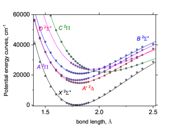
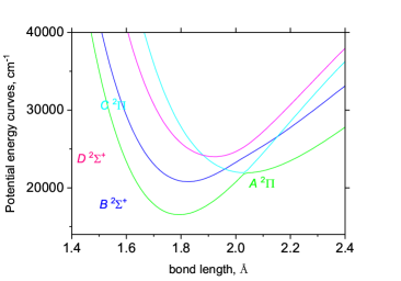
Figure 9: Refined (lines) and ab initio (points) PECs of YO: diabatic (left) and adiabatic (right).

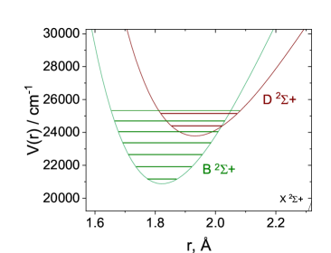
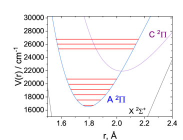
Figure 10: Diabatic PECs of the $B$/$D$ and $A$/$C$ pairs with the corresponding experimental energy term values ($J=0.5$).

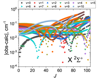
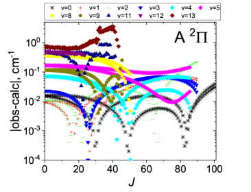
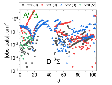
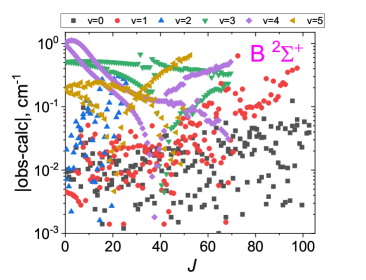
Figure 11: Observed minus calculated residuals for YO using the refined spectroscopic model for different vibronic states.

There are no experimental data on the $C\,{}^{2}\Pi$ state due to its large displacement from the Franck-Condon region of the $X\,{}^{2}\Sigma^{+}$ state. We therefore had to rely on the available ab initio curves associated with this state as well as on their quality. Unlike the CCSD(T) PECs, the corresponding coupling curves were computed with MRCI and are less accurate. Moreover, there is no experimental data representing perturbations caused by the $C\,{}^{2}\Pi$ rovibronic state on other vibronic states in the limited experimental data on YO. However theoretically, using the ab initio data, we do see such perturbations in the $A\,{}^{2}\Pi$, $B\,{}^{2}\Sigma^{+}$ and $D\,{}^{2}\Sigma^{+}$ states due to the spin-orbit and EAM couplings with $C\,{}^{2}\Pi$ (see Smirnov et al. (2019)), which makes the fit especially difficult. We therefore decided to switch off all the coupling with the $C\,{}^{2}\Pi$ state in this work.

The experimental data on the $A^{\prime}\,{}^{2}\Delta$ state is limited to $v=0$ ($J\leq 17.5$), which means only the potential minimum $V_{\rm e}$ of the $A^{\prime}\,{}^{2}\Delta$ state and the corresponding equilibrium constant could be usefully refined, but not its shape, which was fixed to the ab initio CCSD(T) curve via the corresponding EHH potential parameters.

7 Line List

Using our final semi-empirical spectroscopic model, a rovibronic line list of ⁸⁹Y¹⁶O called BRYTS covering the lowest 6 doublet electronic states and the wavelength range up to 166.67 nm was produced. In total 60 678 140 Einstein $A$ coefficients between 173 621 bound rovibronic states were computed with a maximum total rotational quantum number $J_{\text{max}}$ = 400.5. ⁸⁹Y is the only stable isotope of yttrium; however, using the same model, line lists for two minor isotopologues ⁸⁹Y¹⁷O and ⁸⁹Y¹⁸O have been also generated.

The line lists are presented in the standard ExoMol format (Tennyson et al., 2013, 2020) consisting of a States file and a Transitions file with extracts shown in Tables 1 and 2, respectively. The calculated energies in the States file are ‘MARVELised’, i.e. we replace them with the (pseudo-)MARVEL values where available. The uncertainties are taken as the experimental (pseudo-)MARVEL uncertainties for the substituted values, otherwise the following empirical and rather conservative expression is used:

$${\rm unc.}=\Delta T+\Delta\omega\,v+\Delta B\,J(J+1),$$ (17)

with the state-dependent parameters listed in Table 3.

The partition function of YO computed using the new line list is shown in Fig. 12, where it is compared to the partition functions by Barklem & Collet (2016) and Vardya (1970), showing close agreement once a correction is made for the fact that ⁸⁹Y has nuclear spin $\frac{1}{2}$. We also generate temperature- and pressure-dependent opacities of YO using the BRYTS line list and by following the ExoMolOP procedure (Chubb et al., 2021) for four exoplanet atmosphere retrieval codes ARCiS (Min et al., 2020), TauREx (Al-Refaie et al., 2021), NEMESIS (Irwin et al., 2008) and petitRADTRANS (Molliére et al., 2019).

The BRYTS line lists, partition function and opacities are available at www.exomol.com.

Table 1: Extract from the states file of the line list for YO.

$i$	Energy (cm-1)	$g_{i}$	$J$	unc	$\tau$	$g$	Parity		State	$v$	${\Lambda}$	${\Sigma}$	$\Omega$	Ma/Ca	Energy (cm-1)
329	17109.384230	8	1.5	0.060200	0.000000	-0.000268	+	f	A2Pi	1	1	-0.5	0.5	Ma	17109.393106
330	17486.768827	8	1.5	0.220200	0.002928	-0.400448	+	f	X2Sigma+	22	0	0.5	0.5	Ca	17486.768827
331	17538.074400	8	1.5	0.060200	0.000000	0.798897	+	f	A2Pi	1	1	0.5	1.5	Ma	17538.062594
332	17635.333239	8	1.5	4.030000	0.000757	0.399545	+	f	Ap2Delta	4	2	-0.5	1.5	Ca	17635.333239
333	17916.112120	8	1.5	0.110200	0.000000	-0.000268	+	f	A2Pi	2	1	-0.5	0.5	Ma	17916.122345
334	18210.832409	8	1.5	0.230200	0.002827	-0.400448	+	f	X2Sigma+	23	0	0.5	0.5	Ca	18210.832409
335	18345.385550	8	1.5	0.110200	0.000000	0.798904	+	f	A2Pi	2	1	0.5	1.5	Ma	18345.398884
336	18403.241526	8	1.5	5.030000	0.000554	0.399553	+	f	Ap2Delta	5	2	-0.5	1.5	Ca	18403.241526

$i$: State counting number.

$\tilde{E}$: State energy term values in cm^-1, MARVEL or Calculated (Duo).

$g_{i}$: Total statistical weight, equal to ${g_{\rm ns}(2J+1)}$.

$J$: Total angular momentum.

unc: Uncertainty, cm^-1.

$\tau$: Lifetime (s^-1).

$g$: Landé $g$-factors (Semenov et al., 2016).

$+/-$: Total parity.

$e/f$: Rotationless parity.

State: Electronic state.

$v$: State vibrational quantum number.

$\Lambda$: Projection of the electronic angular momentum.

$\Sigma$: Projection of the electronic spin.

$\Omega$: Projection of the total angular momentum, $\Omega=\Lambda+\Sigma$.

Label: ‘Ma’ is for MARVEL and ‘Ca’ is for Calculated.

Energy: State energy term values in cm^-1, Calculated (Duo).

Table 2: Extract from the transitions file of the line list for YO.

$f$	$i$	$A_{fi}$ (s-1)	$\tilde{\nu}_{fi}$
78884	78556	4.1238E+02	10000.000225
111986	112128	6.0427E+01	10000.000489
69517	69133	5.2158E-03	10000.000708
39812	40514	7.3060E-02	10000.000818
34753	33815	6.2941E-04	10000.001400
72754	72910	2.5370E+00	10000.001707
130747	130937	5.3843E-04	10000.002153
130428	130122	1.5407E-02	10000.002287
114934	115604	3.2160E+00	10000.002360
12357	11958	6.2849E+02	10000.002755
135752	135933	1.4867E+01	10000.004338

$f$: Upper state counting number;
$i$: Lower state counting number;
$A_{fi}$: Einstein-$A$ coefficient in s^-1;
$\tilde{\nu}_{fi}$: transition wavenumber in cm^-1.

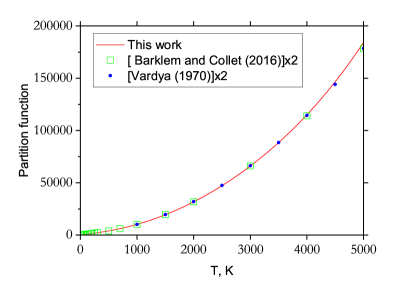
Figure 12: Partition functions of YO: From this work (solid line), from Vardya (1970) (filled circles) and from Barklem & Collet (2016) (open squares). The latter two were multiplied by a factor of 2 to account for the different treatment of nuclear statistics.

Table 3: Parameters used to estimate uncertainties of the YO calculated energy term values according to Eq. (17).

State	$\Delta T$	$\Delta\omega$	$\Delta B$
$X\,{}^{2}\Sigma^{+}$	0.0	0.01	0.0001
$A\,{}^{2}\Pi$	0.01	0.05	0.0001
$C\,{}^{2}\Pi$	10.0	1.0	0.01
$B\,{}^{2}\Sigma^{+}$	0.01	0.057	0.0001
$D\,{}^{2}\Sigma^{+}$	0.01	0.07	0.0001
$A^{\prime}\,{}^{2}\Delta$	0.01	1	0.01

8 Simulated Spectra

Using the computed line list for YO, here we simulate the YO rovibronic absorption spectra using the program ExoCross (Yurchenko et al., 2018b). Fig. 13 shows the temperature variation of the YO rovibronic spectrum over the spectroscopic range up to 166 nm. Figure 14 highlights the contribution of the most important electronic bands to the total opacity simulated at 2000 K such that there is good separation between the electronic bands. In both simulations, each line was broadened using a Lorentzian line profile with a HWHM of 1 cm^-1 and computed at a resolution of 1 cm^-1.

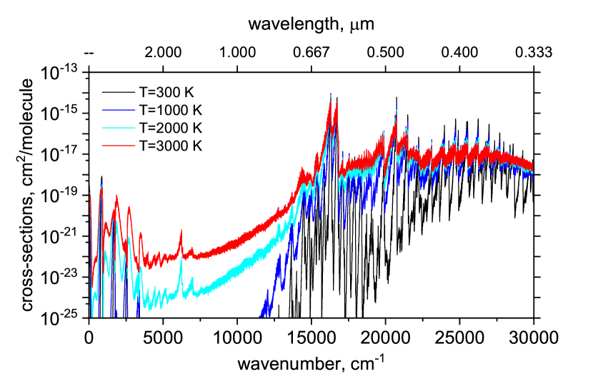
Figure 13: The simulated YO absorption spectrum computed at different temperatures. We adopt a Lorentzian line broadening of 1 cm^-1 for each line which is computed at a resolution of 1 cm^-1. We see the intensity deviation is greatest around 0.5 and 0.6 $\mu$m where the $X\,{}^{2}\Sigma^{+}$$\rightarrow$$A\,{}^{2}\Pi$ and $X\,{}^{2}\Sigma^{+}$$\rightarrow$$B\,{}^{2}\Sigma^{+}$  bands dominate opacity.

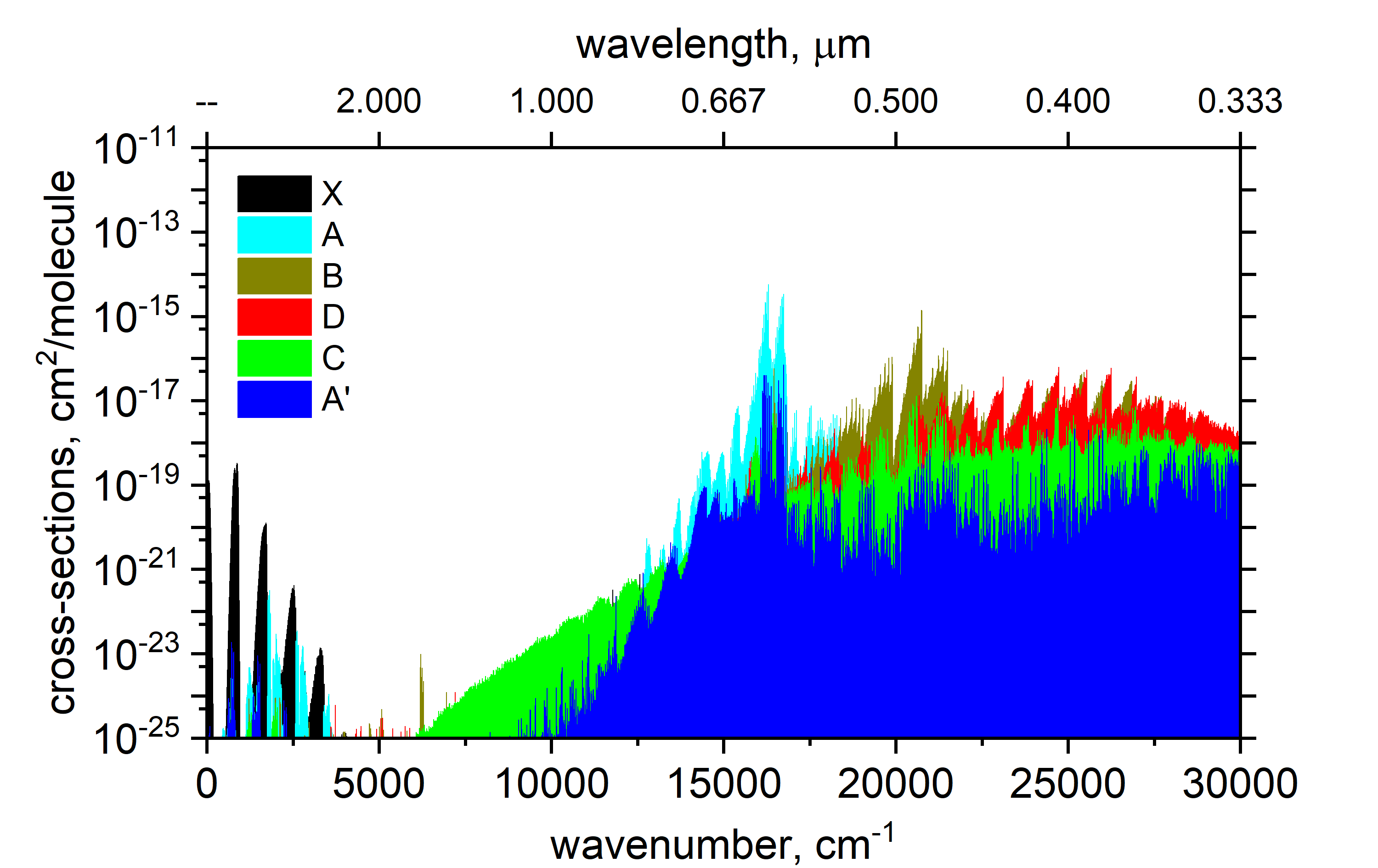
Figure 14: Different electronic band components of the absorption spectrum simulated at 2000 K using Lorentzian line broadening of 1 cm^-1 for each line computed at a resolution of 1 cm^-1.

8.1 Lifetimes

Table 4 compares our lifetimes to the experimental and theoretical values from the literature: laser fluorescence measurements of the $A\,{}^{2}\Pi$ and $B\,{}^{2}\Sigma^{+}$ states ($v\leq 2$) of YO by Liu & Parson (1977) and $B\,{}^{2}\Sigma^{+}$ ($v=0$) and $D\,{}^{2}\Sigma^{+}$ ($v=0,1$) lifetimes by Zhang et al. (2017) as well as to the theoretical values by Langhoff & Bauschlicher (1988) and Smirnov et al. (2019). The theoretical values correspond to the lowest $J$ values, $J=0.5$ for $X\,{}^{2}\Sigma^{+}$, $B\,{}^{2}\Sigma^{+}$ and $D\,{}^{2}\Sigma^{+}$, $J=1.5$ for $A\,{}^{2}\Pi$ and $C\,{}^{2}\Pi$, $J=1.5$ for $A^{\prime}\,{}^{2}\Delta$  which we consider as a good proxy for the experimental values ($J$ unspecified) due to very slow $J$ dependence of the lifetimes. The good agreement is partly due to the adjustment of the corresponding TDMC to match the corresponding lifetimes as specified above. Our result is the best we could do for a complicated system $D\,{}^{2}\Sigma^{+}$–$X\,{}^{2}\Sigma^{+}$ with a complex diabatic coupling (Fig. 3) and the diabatised $D\,{}^{2}\Sigma^{+}$–$X\,{}^{2}\Sigma^{+}$  TDMC based on some level of arbitrariness (Fig. 7).

Table 4: Lifetimes of ⁸⁹Y¹⁶O states in ns: comparison with the measurements of [77LiPa] (Liu & Parson, 1977) and [17ZhZhZh] (Zhang et al., 2017), and the ab initio calculations of [19SmSoYu] (Smirnov et al., 2019).

State	$v$	[77LiPa]	[17ZhZhZh]	[19SmSoYu]	This work
$A\,{}^{2}\Pi$1/2	$0$	$33.0\pm 1.3$		$22.6$	$35.5$
	$1$	$36.5\pm 2.4$		$23.0$	$36.1$
$A\,{}^{2}\Pi$3/2	$0$	$32.3\pm 0.9$		$20.9$	$32.7$
	$1$	$30.4\pm 1.8$		$21.3$	$33.3$
	$2$	$33.4\pm 1.5$		$21.6$	$33.9$
	$6$	$41.6\pm 2.1$		$29.2$	$37.3$
$B\,{}^{2}\Sigma^{+}$	$0$	$30.0\pm 0.9$	$38\pm 5$	$32.5$	$30.7$
	$1$	$32.5\pm 1.2$		$34.3$	$30.4$
$D\,{}^{2}\Sigma^{+}$	$0$		$79\pm 5$	$30.1$	$62.5$
	$1$		$79\pm 5$	$29.2$	$56.8$

9 Comparisons To Experimental Spectra

Figure 15 compares the experimental $A\,{}^{2}\Pi$_1/2$\xrightarrow[]{}$$X\,{}^{2}\Sigma^{+}$ $v=0\rightarrow 0$ emission bands measured by Bernard et al. (1979) via Fourier Transform spectroscopy (black, extracted from their Fig. 2) to our computed spectra (red). We simulate our spectra at the temperature of 1500 K to agree with the rotational structure of the experiment. We see excellent agreement in both line position and band structure with the experiment. Some discrepancies can be seen in the line intensities, but this could be due to our assumptions about the temperature and line broadening. Table 5 provides an extended comparisons of the positions of band heads of the $A\,{}^{2}\Pi$–$X\,{}^{2}\Sigma^{+}$ system between the experimental values reported by Bernard & Gravina (1983) and the theoretical values from the present work, as well as the corresponding values of $J_{\rm head}$. Generally, the magnitude of residuals $\Delta\tilde{\nu}=\tilde{\nu}_{\rm exp}-\tilde{\nu}_{\rm calc}$ correlates with the level of the rotational and vibrational excitations. The band heads with $J_{\rm head}$ below $70.5$ and $v\leq 8$ agree within $\sim 0.1$ cm^-1, which then degrades to about 0.5 cm^-1 for $J_{\rm head}\to 100.5$.

As in Smirnov et al. (2019), for the sake of completeness, we provide comparisons with the emission $A^{\prime}\,{}^{2}\Delta$ – $X\,{}^{2}\Sigma^{+}$ spectrum from Simard et al. (1992), Fig. 16, and the $B\,{}^{2}\Sigma^{+}$ – $X\,{}^{2}\Sigma^{+}$ and $D\,{}^{2}\Sigma^{+}$ – $X\,{}^{2}\Sigma^{+}$ absorption spectra from Zhang et al. (2017), Fig. 17, using the BRYTS line list, now with an improved agreement, see also the corresponding discussions in Smirnov et al. (2019). Figure Fig. 17 shows the simulation of the the forbidden band $A^{\prime}\,{}^{2}\Delta$ – $X\,{}^{2}\Sigma^{+}$ (0,0) in emission. In Fig. 17, non-local thermodynamic equilibrium conditions with the rotational temperature $T_{\rm rot}$ = 50 K and the vibrational temperature of $T_{\rm vib}$ = 800 K to better reproduce the experimental spectrum were assumed.

Table 5: Comparison of the experimental (Bernard & Gravina, 1983) and theoretical (this work) positions of the band heads in the $A\,{}^{2}\Pi$–$X\,{}^{2}\Sigma^{+}$ system.

$v^{\prime}$	$v^{\prime\prime}$	branch	$J_{\rm head}$ (obs)	$J_{\rm head}$ (calc)	$\tilde{\nu}_{\rm exp}$	$\tilde{\nu}_{\rm calc}$	$\Delta\tilde{\nu}$
0	1	$Q_{1}$	93.5	98.5	15456.10	15456.61	-0.51
1	2	$Q_{1}$	87.5	88.5	15417.24	15417.45	-0.21
2	3	$Q_{1}$	77.5	79.5	15377.56	15377.77	-0.21
3	4	$Q_{1}$	70.5	71.5	15337.30	15337.45	-0.15
4	5	$Q_{1}$	62.5	63.5	15296.26	15296.37	-0.11
5	6	$Q_{1}$	56.5	56.5	15254.24	15254.41	-0.17
6	7	$Q_{1}$	49.5	50.5	15210.78	15211.28	-0.50
8	9	$Q_{1}$	37.5	39.5	15123.48	15123.34	0.14
9	10	$Q_{1}$	33.5	35.5	15077.15	15077.28	-0.13
10	11	$Q_{1}$		27.5	15033.33	15030.30	3.03
11	12	$Q_{1}$		25.5	14981.00	14981.17	-0.17
12	13	$Q_{1}$		26.5	14933.83	14934.60	-0.77
13	14	$Q_{1}$		23.5	14880.28	14882.94	-2.66
14	15	$Q_{1}$		19.5	14829.85	14832.44	-2.59
15	16	$Q_{1}$		18.5	14774.01	14778.50	-4.49
16	17	$Q_{1}$		18.5	14718.59	14725.27	-6.68
17	18	$Q_{1}$		17.5	14654.49	14671.33	-16.84
18	19	$Q_{1}$		16.5	14615.68	14616.53	-0.85
20	21	$Q_{1}$		63.5	14535.74	14541.80	-6.06
21	22	$Q_{1}$		59.5	14494.52	14479.62	14.90
22	23	$Q_{1}$		54.5	14452.30	14416.66	35.64
0	0	$Q_{1}$	51.5	51.5	16303.10	16303.16	-0.06
0	0	$R_{2}$	79.5	81.5	16739.90	16740.01	-0.11
1	1	$Q_{1}$	47.5	48.5	16259.93	16259.89	0.04
1	1	$R_{2}$	72.5	74.5	16696.30	16696.36	-0.06
2	2	$Q_{1}$	44.5	44.5	16215.91	16215.89	0.02
2	2	$R_{2}$	66.5	68.5	16652.15	16652.10	0.05
3	3	$Q_{1}$	40.5	41.5	16171.00	16171.02	-0.02
3	3	$R_{2}$	61.5	62.5	16607.07	16607.07	0.00
4	4	$Q_{1}$	37.5	37.5	16125.08	16125.20	-0.12
4	4	$R_{2}$	56.5	57.5	16561.11	16561.16	-0.05
5	5	$Q_{1}$	34.5	35.5	16078.10	16078.30	-0.20
5	5	$R_{2}$	51.5	52.5	16514.06	16514.08	-0.02
6	6	$Q_{1}$	31.5	32.5	16029.60	16030.15	-0.55
6	6	$R_{2}$		35.5	16462.40	16462.74	-0.34
7	7	$R_{2}$	43.5	44.5	16417.60	16418.85	-1.25
8	8	$Q_{1}$	26.5	27.5	15932.00	15931.69	0.31
8	8	$R_{2}$	37.5	37.5	16367.89	16370.33	-2.44
9	9	$Q_{1}$	24.5	25.5	15880.20	15880.17	0.03
9	9	$R_{2}$	33.5	35.5	16315.88	16317.95	-2.07
10	10	$Q_{1}$		22.5	15828.06	15827.76	0.30
11	11	$Q_{1}$		19.5	15773.23	15773.03	0.20
12	12	$Q_{1}$		20.5	15720.30	15720.47	-0.17

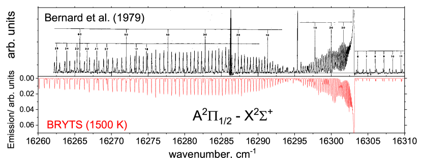
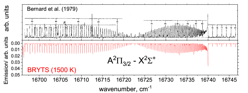
Figure 15: Comparison of our computed $A\,{}^{2}\Pi$_1/2 $\rightarrow$ $X\,{}^{2}\Sigma^{+}$  and $A\,{}^{2}\Pi$_3/2 $\rightarrow$ $X\,{}^{2}\Sigma^{+}$  rotational-electronic emission bands (79BeBaLu, red lines) with those of Bernard et al. (1979), a measured spectrum using Fourier Transform Spectroscopy (upper displays). We compute our spectrum at a temperature of 1500 K to best match that of Bernard et al. (1979). A Gaussian line profile of 0.065 cm^-1 was used with a resolution of 0.01 cm^-1. ©AAS. Reproduced with permission.

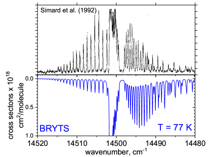
Figure 16: Comparison of the computed emission $A^{\prime}\,{}^{2}\Delta$ – $X\,{}^{2}\Sigma^{+}$ (0,0) band with the measurements of Simard et al. (1992) at $T=77$ K and Lorentzian line profile of HWHM = 0.04 cm^-1.

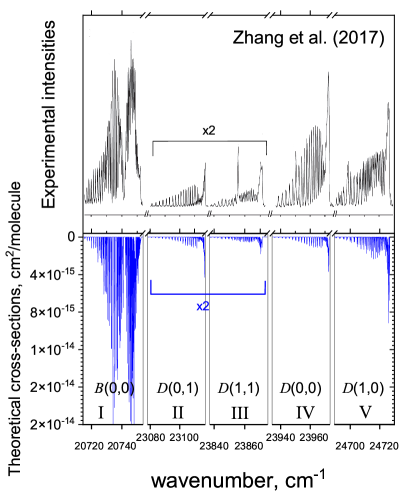
Figure 17: Comparison of our computed (bottom) $D\,{}^{2}\Sigma^{+}$–$X\,{}^{2}\Sigma^{+}$ absorption spectra to the measurements of Zhang et al. (2017) (top). The simulations assumed a cold rotational temperature of $T_{\rm rot}$ = 50 K and a hot vibrational temperature of $T_{\rm vib}$ = 800 K. A Doppler line profile corresponding to $T_{\rm rot}$ = 50 K was used.

10 Conclusions

Accurate and extensive empirical BRYTS line lists for ⁸⁹Y¹⁶O, ⁸⁹Y¹⁷O and ⁸⁹Y¹⁸O are produced covering six lowest doublet electronic states and ranging up to 60 000 cm^-1. The line list is based on a refined set of curves in the diabatic representation obtained by fitting to a set of experimentally derived rovibronic energies of YO. The latter is based on the experimental data from the literature, either original laboratory line positions whenever available or spectroscopic constants. Using an effective Hamiltonian to reconstruct molecular energies in place of the original experimental data is less than ideal as it lacks information on any local perturbations, which is critical when using it to fit the spectroscopic model.

Although ExoMol line lists, including BRYTS, are usually intended for astrophysical applications of hot atmospheric environments, YO is one of the molecules used in cooling applications, where our line list may also be useful.

The ab initio calculations, especially MRCI, of transition metal species are still a big challenge and therefore ultimately the lab data (transition frequencies, intensities, dipoles, lifetimes) is a crucial source of the information to produce useful line lists. For YO we were lucky to have the ab initio PECs of excited electronic states of the CCSD(T) quality, while everything else had to rely on the fit to the experiment.

In this work, the hyperfine structure of the YO rovibronic states was ignored, mostly due to the lack of the experiment. Should it become important for YO spectroscopic applications to include the hyperfine effects, the methodology to compute the hyperfine-resolved energies and spectra is readily available as implemented in Duo (Qu et al., 2022a, b; Bowesman et al., 2023).

Data Availability

The states, transition, opacity and partition function files for the YO line lists can be downloaded from www.exomol.com. The open access programs Duo and ExoCross are available from github.com/exomol.

Supporting Information

Supplementary data are available at MNRAS online. This includes (i) the spectroscopic model in the form of the Duo input file, containing all the curves, parameters as well as the experimentally derived energy term values of YO used in the fit; (ii) the experimental line positions collected from the literature in the MARVEL format and (iii) an effective Hamiltonian for a ${}^{2}\Pi$ electronic state from Bacis et al. (1977).

References

- Ackermann & Rauh (1974) Ackermann R. J., Rauh E. G., 1974, J. Chem. Phys., 60, 2266
- Al-Refaie et al. (2021) Al-Refaie A. F., Changeat Q., Waldmann I. P., Tinetti G., 2021, ApJ, 917, 37
- Bacis et al. (1977) Bacis R., Cerny D., D’Incan J., Guelachvili G., Roux F., 1977, ApJ, 214, 946
- Badie & Granier (2002) Badie J. M., Granier B., 2002, Chem. Phys. Lett., 364, 550
- Badie & Granier (2003) Badie J. M., Granier B., 2003, Eur. Phys. J.-Appl. Phys, 21, 239
- Badie et al. (2005a) Badie J. M., Cassan L., Granier B., 2005a, Eur. Phys. J.-Appl. Phys, 29, 111
- Badie et al. (2005b) Badie J. M., Cassan L., Granier B., 2005b, Eur. Phys. J.-Appl. Phys, 32, 61
- Badie et al. (2007a) Badie J. M., Cassan L., Granier B., 2007a, Eur. Phys. J.-Appl. Phys, 38, 177
- Badie et al. (2007b) Badie J. M., Cassan L., Granier B., Florez S. A., Janna F. C., 2007b, J. Sol. Energy Eng. Trans.-ASME, 129, 412
- Bagare & Murthy (1982) Bagare S. P., Murthy N. S., 1982, Pramana, 19, 497
- Barklem & Collet (2016) Barklem P. S., Collet R., 2016, A&A, 588, A96
- Bernard & Gravina (1980) Bernard A., Gravina R., 1980, ApJS, 44, 223
- Bernard & Gravina (1983) Bernard A., Gravina R., 1983, ApJS, 52, 443
- Bernard et al. (1979) Bernard A., Bacis R., Luc P., 1979, ApJ, 227, 338
- Bowesman et al. (2023) Bowesman C. A., Yurchenko S. N., Tennyson J., 2023, Mol. Phys.
- Brady et al. (2022) Brady R. P., Yurchenko S. N., Kim G.-S., Somogyi W., Tennyson J., 2022, Phys. Chem. Chem. Phys., 24, 24076
- Brady et al. (2023) Brady R. P., Drury C., Tennyson J., Yurchenko S. N., 2023, Mol. Phys., in preparation
- Brown & Merer (1979) Brown J. M., Merer A. J., 1979, J. Mol. Spectrosc., 74, 488
- Cazzoli et al. (2006) Cazzoli G., Cludi L., Puzzarini C., 2006, J. Mol. Struct., 780-81, 260
- Chalek & Gole (1976) Chalek C. L., Gole J. L., 1976, J. Chem. Phys., 65, 2845
- Chalek & Gole (1977) Chalek C. L., Gole J. L., 1977, Chem. Phys., 19, 59
- Childs et al. (1988) Childs W. J., Poulsen O., Steimle T. C., 1988, J. Chem. Phys., 88, 598
- Chubb et al. (2021) Chubb K. L., et al., 2021, A&A, 646, A21
- Collopy et al. (2015) Collopy A. L., Hummon M. T., Yeo M., Yan B., Ye J., 2015, New J. Phys, 17, 055008
- Collopy et al. (2018) Collopy A. L., Ding S., Wu Y., Finneran I. A., Anderegg L., Augenbraun B. L., Doyle J. M., Ye J., 2018, Phys. Rev. Lett., 121, 213201
- Dye et al. (1991) Dye R. C., Muenchausen R. E., Nogar N. S., 1991, Chem. Phys. Lett., 181, 531
- Fried et al. (1993) Fried D., Kushida T., Reck G. P., Rothe E. W., 1993, J. Appl. Phys., 73, 7810
- Furtenbacher et al. (2007) Furtenbacher T., Császár A. G., Tennyson J., 2007, J. Mol. Spectrosc., 245, 115
- Goranskii & Barsukova (2007) Goranskii V. P., Barsukova E. A., 2007, Astron. Rep., 51, 126
- Hoeft & Torring (1993) Hoeft J., Torring T., 1993, Chem. Phys. Lett., 215, 367
- Hulburt & Hirschfelder (1941) Hulburt H. M., Hirschfelder J. O., 1941, J. Chem. Phys., 9, 61
- Irwin et al. (2008) Irwin P. G. J., et al., 2008, J. Quant. Spectrosc. Radiat. Transf., 109, 1136
- Kaminski et al. (2009) Kaminski T., Schmidt M., Tylenda R., Konacki M., Gromadzki M., 2009, ApJS, 182, 33
- Kasai & Weltner (1965) Kasai P. H., Weltner Jr. W., 1965, J. Chem. Phys., 43, 2553
- Knight et al. (1999) Knight L. B., Kaup J. G., Petzoldt B., Ayyad R., Ghanty T. K., Davidson E. R., 1999, J. Chem. Phys., 110, 5658
- Kobayashi & Sekine (2006) Kobayashi T., Sekine T., 2006, Chem. Phys. Lett., 424, 54
- Langhoff & Bauschlicher (1988) Langhoff S. R., Bauschlicher C. W., 1988, J. Chem. Phys., 89, 2160
- Lee et al. (1999) Lee E. G., Seto J. Y., Hirao T., Bernath P. F., Le Roy R. J., 1999, J. Mol. Spectrosc., 194, 197
- Leung et al. (2005) Leung J. W. H., Ma T. M., Cheung A. S. C., 2005, J. Mol. Spectrosc., 229, 108
- Linton (1978) Linton C., 1978, J. Mol. Spectrosc., 69, 351
- Liu & Parson (1977) Liu K., Parson J. M., 1977, J. Chem. Phys., 67, 1814
- Liu & Parson (1979) Liu K., Parson J. M., 1979, J. Phys. Chem., 83, 970
- Manos & Parson (1975) Manos D. M., Parson J. M., 1975, J. Chem. Phys., 63, 3575
- Medvedev (2012) Medvedev E. S., 2012, J. Chem. Phys., 137, 174307
- Medvedev & Ushakov (2022) Medvedev E. S., Ushakov V. G., 2022, J. Quant. Spectrosc. Radiat. Transf., 288, 108255
- Medvedev et al. (2015) Medvedev E. S., Meshkov V. V., Stolyarov A. V., Gordon I. E., 2015, J. Chem. Phys., 143, 154301
- Medvedev et al. (2016) Medvedev E. S., Meshkov V. V., Stolyarov A. V., Ushakov V. G., Gordon I. E., 2016, J. Mol. Spectrosc., 330, 36
- Min et al. (2020) Min M., Ormel C. W., Chubb K., Helling C., Kawashima Y., 2020, A&A, 642, A28
- Molliére et al. (2019) Molliére P., Wardenier J. P., van Boekel R., Henning T., Molaverdikhani K., Snellen I. A. G., 2019, A&A, 627, A67
- Mukund & Nakhate (2023) Mukund S., Nakhate S. G., 2023, J. Quant. Spectrosc. Radiat. Transf., 296, 108452
- Murty (1982) Murty P. S., 1982, Astrophys. Lett., 23, 7
- Murty (1983) Murty P. S., 1983, Astrophys. Space Sci., 94, 295
- Otis & Goodwin (1993) Otis C. E., Goodwin P. M., 1993, J. Appl. Phys., 73, 1957
- Peterson & Dunning (2002) Peterson K. A., Dunning T. H., 2002, J. Chem. Phys., 117, 10548
- Peterson et al. (2007) Peterson K. A., Figgen D., Dolg M., Stoll H., 2007, J. Chem. Phys., 126, 124101
- Prajapat et al. (2017) Prajapat L., Jagoda P., Lodi L., Gorman M. N., Yurchenko S. N., Tennyson J., 2017, MNRAS, 472, 3648
- Qu et al. (2022a) Qu Q., Yurchenko S. N., Tennyson J., 2022a, J. Chem. Theory Comput., 18, 1808
- Qu et al. (2022b) Qu Q., Yurchenko S. N., Tennyson J., 2022b, J. Chem. Phys., 157, 124305
- Quéméner & Bohn (2016) Quéméner G., Bohn J. L., 2016, Phys. Rev. A, 93, 012704
- Sauval (1978) Sauval A. J., 1978, A&A, 62, 295
- Semenov et al. (2016) Semenov M., Yurchenko S. N., Tennyson J., 2016, J. Mol. Spectrosc., 330, 57
- Shin & Nicholls (1977) Shin J. B., Nicholls R. W., 1977, Spectr. Lett., 10, 923
- Simard et al. (1992) Simard B., James A. M., Hackett P. A., Balfour W. J., 1992, J. Mol. Spectrosc., 154, 455
- Smirnov et al. (2019) Smirnov A. N., Solomonik V. G., Yurchenko S. N., Tennyson J., 2019, Phys. Chem. Chem. Phys., 21, 22794
- Steimle & Alramadin (1986) Steimle T. C., Alramadin Y., 1986, Chem. Phys. Lett., 130, 76
- Steimle & Alramadin (1987) Steimle T. C., Alramadin Y., 1987, J. Mol. Spectrosc., 122, 103
- Steimle & Shirley (1990) Steimle T. C., Shirley J. E., 1990, J. Chem. Phys., 92, 3292
- Steimle & Virgo (2003) Steimle T. C., Virgo W., 2003, J. Mol. Spectrosc., 221, 57
- Suenram et al. (1990) Suenram R. D., Lovas F. J., Fraser G. T., Matsumura K., 1990, J. Chem. Phys., 92, 4724
- Tennyson & Yurchenko (2012) Tennyson J., Yurchenko S. N., 2012, MNRAS, 425, 21
- Tennyson et al. (2013) Tennyson J., Hill C., Yurchenko S. N., 2013, in 6th international conference on atomic and molecular data and their applications ICAMDATA-2012. AIP, New York, pp 186–195, doi:10.1063/1.4815853
- Tennyson et al. (2020) Tennyson J., et al., 2020, J. Quant. Spectrosc. Radiat. Transf., 255, 107228
- Tylenda et al. (2015) Tylenda R., Górny S. K., Kamínski T., Schmidt M., 2015, A&A, 578, A75
- Uhler & Akerlind (1961) Uhler U., Akerlind L., 1961, Arkiv For Fysik, 19, 1
- Ushakov et al. (2023) Ushakov V., Semenov M., Yurchenko S., Ermilov A. Y., Medvedev E., 2023, J. Mol. Spectrosc., p. 111804
- Vardya (1970) Vardya M. S., 1970, A&A, 5, 162
- Werner et al. (2020) Werner H.-J., et al., 2020, The Journal of Chemical Physics, 152, 144107
- Western (2017) Western C. M., 2017, J. Quant. Spectrosc. Radiat. Transf., 186, 221
- Wijchers et al. (1980) Wijchers T., Dijkerman H. A., Zeegers P. J. T., Alkemade C. T. J., 1980, Spectra Chimica Acta B, 35, 271
- Wijchers et al. (1984) Wijchers T., Dijkerman H. A., Zeegers P. J. T., Alkemade C. T. J., 1984, Chem. Phys., 91, 141
- Wyckoff & Clegg (1978) Wyckoff S., Clegg R. E. S., 1978, MNRAS, 184, 127
- Yeo et al. (2015) Yeo M., Hummon M. T., Collopy A. L., Yan B., Hemmerling B., Chae E., Doyle J. M., Ye J., 2015, Phys. Rev. Lett., 114, 223003
- Yurchenko et al. (2016) Yurchenko S. N., Lodi L., Tennyson J., Stolyarov A. V., 2016, Comput. Phys. Commun., 202, 262
- Yurchenko et al. (2018a) Yurchenko S. N., Sinden F., Lodi L., Hill C., Gorman M. N., Tennyson J., 2018a, MNRAS, 473, 5324
- Yurchenko et al. (2018b) Yurchenko S. N., Al-Refaie A. F., Tennyson J., 2018b, A&A, 614, A131
- Yurchenko et al. (2022) Yurchenko S. N., Nogué E., Azzam A. A. A., Tennyson J., 2022, MNRAS, 520, 5183
- Zhang et al. (2017) Zhang D., Zhang Q., Zhu B., Gu J., Suo B., Chen Y., Zhao D., 2017, J. Chem. Phys., 146, 114303