Comprehensive Assessment of the Performance of Deep Learning Classifiers Reveals a Surprising Lack of Robustness

Abstract

Reliable and robust evaluation methods are a necessary first step towards developing machine learning models that are themselves robust and reliable. Unfortunately, current evaluation protocols typically used to assess classifiers fail to comprehensively evaluate performance as they tend to rely on limited types of test data, and ignore others. For example, using the standard test data fails to evaluate the predictions made by the classifier to samples from classes it was not trained on. On the other hand, testing with data containing samples from unknown classes fails to evaluate how well the classifier can predict the labels for known classes. This article advocates bench-marking performance using a wide range of different types of data and using a single metric that can be applied to all such data types to produce a consistent evaluation of performance. Using such a benchmark it is found that current deep neural networks, including those trained with methods that are believed to produce state-of-the-art robustness, are extremely vulnerable to making mistakes on certain types of data. This means that such models will be unreliable in real-world scenarios where they may encounter data from many different domains, and that they are insecure as they can easily be fooled into making the wrong decisions. It is hoped that these results will motivate the wider adoption of more comprehensive testing methods that will, in turn, lead to the development of more robust machine learning methods in the future.

Keywords:

deep learning, neural networks, classification, generalisation, robustness, out-of-distribution, open-set, common corruptions, adversarial training, data augmentation

1 Introduction

1.1 Need for Robustness

The tremendous success of deep learning (DL) makes it easy to overlook the fact that such models are often extremely brittle and insufficiently reliable for deployment in real-world scenarios, particularly in domains where security, safety, or trust are concerns (Amodei et al., 2016; Heaven, 2019; Serre, 2019; Yuille and Liu, 2021; Bowers et al., 2023; Marcus, 2020). This lack of robustness is illustrated in Fig. 1, using the domain of image classification as an example. Essentially DL, and more generally machine learning (ML) and artificial intelligence (AI), is poor at correctly generalising to novel data/situations. However, to be dependable it is essential that such methods be able to make accurate predictions on data that was not used for training, i.e., for the trained model to generalise to novel, unseen, data.

1.2 Types of Robustness

True class=

Prediction=

IID

Generalisation

(clean accuracy)

phone

✓ phone ✓

OOD

Generalisation

(corrupt accuracy)

phone

✗ radio ✗

Adversarial Robustness

(adversarial acc.)

phone

✗ radio ✗

OOD Detection

(novel class rejection)

unknown

✗ phone ✗

OOD Detection

(unrecognisable image rejection)

unknown

✗ phone ✗

Figure 1: A synthetic example of the sort of predictions made by a deep learning classifier when tested in different ways after being trained to recognise images of objects from categories including “phone” and “radio”. Each sub-figure illustrates a different method of testing the accuracy of the classifier, it shows four sample images and the ground-truth and predicted classes for those images. (a) Samples from the test/validation data-set (this data looks very similar to the training data). (b) Samples used to assess generalisation. (c) Adversarially perturbed samples (the modifications to the images are virtually imperceptible but cause significant change to the classifier’s prediction). (d) Samples showing objects from categories not included in the training data. (e) Samples that differ from images of natural objects or that have been synthetically generated to fool the classifier into making incorrect, high confidence, predictions. (Figure inspired by Fig. 1 of Kumano et al., 2022).

The ability to generalise can be assessed in multiple ways. Firstly, generalisation performance can be assessed using a test or validation set (see Fig. 1a). Such data is typically similar to the training data as it is drawn from the same distribution in the input feature-space. This assessment method is thus said to measure in-distribution generalisation, or generalisation to independent and identically distributed (IID) samples. Such data is routinely used to assess the performance of classifiers.

A more challenging form of generalisation is out-of-distribution (OOD) generalisation (see Fig. 1b). This can be assessed using test data that has different characteristics than the training data, but the same class labels. For example, in the domain of image categorisation it might be necessary for the classifier to cope with changes in appearance caused by images being captured under different conditions to those used to capture the training images. This can result in variations in orientation, scale, viewpoint, background, clutter, lighting, blur, jpg compression, image resolution, etc.. Furthermore, to succeed at OOD generalisation the classifier should ideally be tolerant to changes in appearance due to within-class variations, and for certain types of object (such as human bodies) non-rigid deformations. For image classification tasks, OOD generalisation can be assessed using clean samples that have been deliberately chosen because they differ from the training data (Zhang et al., 2023; Hendrycks et al., 2021a; Hendrycks and Dietterich, 2019; Li et al., 2017) or using IID test images that have been synthetically modified, or corrupted, to simulate changes in image capture conditions (Michaelis et al., 2019; Hendrycks et al., 2021b; Mu and Gilmer, 2019; Hendrycks and Dietterich, 2019; Jansson and Lindeberg, 2020).

The limits placed on such generalisation may be task-dependent. For example, the image on the bottom-right of Fig. 1b shows a phone with a smashed screen. If the task were classification then this image should be identified as a phone, even if no training image showed an exemplar with a broken screen. However, if the task being performed was anomaly detection (i.e., finding defects in objects) then this exemplar would need to be identified as an anomaly. OOD generalisation is closely related to the task of domain generalisation (DG), although DG typically employs multiple training data-sets from different domains to train a method to generalise to an unseen target domain. In turn DG is closely related to domain adaptation (DA), although DA allows access to (a limited amount of) training data from the target domain to improve model transfer (Wang et al., 2022; Riaz and Smeaton, 2023).

A third method of assessing generalisation performance is through the use of adversarial exemplars (see Fig. 1c). These are clean, in-distribution, samples that have been modified (or “perturbed”) in such a way as to cause a change in the predicted class even when the class of the perturbed input appears unchanged to a human observer (Akhtar and Mian, 2018; Szegedy et al., 2014; Goodfellow et al., 2015; Kurakin et al., 2017; Eykholt et al., 2018; Biggio and Roli, 2018). Adversarial perturbations have the appearance of low-amplitude random noise, and can be generated using a wide range of different algorithms (Liang et al., 2022; Ren et al., 2020; Xu et al., 2020) which attempt to find small changes in the inputs that cause large changes in the predictions of the classifier.

A fourth requirement for robust ML is the ability to reject samples from categories that were not seen during training (see Fig. 1d). Current DL models are susceptible to producing high-confidence, but incorrect, predictions to samples that are far from the training data distribution (Amodei et al., 2016; Hendrycks and Gimpel, 2017). The susceptibility of a classifier to making such errors can be evaluated simply by measuring its response to samples taken from data-sets containing classes distinct from those used for training. The task of creating classifiers that are less susceptible to making such errors is called open-set recognition (OSR; Vaze et al., 2022; Yang et al., 2022) or OOD detection/rejection (Mohseni et al., 2020; Hendrycks and Gimpel, 2017; Bitterwolf et al., 2022; Zhang and Ranganath, 2023; Hendrycks et al., 2022).

Finally, another situation in which an image classifier may produce high-confidence, but incorrect, predictions is when tested with exemplars that are unlike images of any object. Typically, synthetic images that occupy regions in feature-space that are far from those occupied by natural images, and hence, appear to human observers to have no similarity to the class label predicted by the classifier (see Fig. 1e). Such images can be created using stochastic processes, or like adversarial exemplars, can be algorithmically generated to deliberately fool the classifier. This latter category, known as “fooling images”, may look like noise (Hendrycks and Gimpel, 2017), or textures (Nguyen et al., 2015), or images that are uniform except for a few differently coloured pixels (Kumano et al., 2022).

The two images at the bottom-left of Fig. 1b and d, illustrate a fundamental difficulty of accurate classification. It is necessary to have tolerance to within-class variation, and other changes in image capture conditions, so that visually dissimilar images can be allocated to the same class, while simultaneously being able to make fine-grained distinctions so that similar looking images from different classes can be distinguished (Bar, 2004).

1.3 Terminology

OOD generalisation is concerned with classifying data where the distribution of the input (i.e., the characteristics of the images) has changed, but the distribution of output (i.e., the range of class labels associated with the images) is constant. In contrast OOD rejection is concerned with identifying data where the distribution of both the input and output has changed. The term “distribution” is therefore being used to refer to different distributions in each case. For OOD generalisation it is the distribution of the input, while for OOD rejection it is primarily the distribution of the output (the change in the input distribution is simply a side-effect of the change to new class labels). To avoid any possible confusion, OOD detection/rejection will hence-forth be referred to as “Unknown Class Rejection”. The data used to assess unknown class rejection will be subdivided into “novel” classes (images containing objects from classes unseen during training) and “unrecognisable” images (those containing no sematically meaningful information).

The term “distribution” when applied to the input is also poorly defined and, arguably, irrelevant when discussing IID/OOD generalisation. All data other than that included in the training set is OOD for the classifier, so the distinction between IID and OOD data is qualitative rather than quantitative, and the boundary between in- and out-of distribution is necessarily arbitrary. Furthermore, the shift in distribution in image-space often has little correlation with the difficulty in correctly classifying an image. For example, two images of the same object taken from different viewpoints may have very little similarity in terms of corresponding pixels values, but the images may be easily identified as containing the same object. In contrast, it may be very difficult for the classifier to assign the same label to two images that are almost identical in image-space (e.g., a clean image and an adversarially perturbed version of that same image). Most importantly, how far an image is from the training distribution is irrelevant to the task of the classifier. Ideally, the classifier should be able to successfully recognise novel exemplars of the objects it was trained on however similar or dissimilar they are in appearance to the images used in training. In contrast an ideal classifier should reject images containing unknown objects even if such images are close to the training distribution. Hence, rather than using the terms IID and OOD, the remaining text will refer to such data as being from “known” classes. The broad class of known data will be sub-divided into different types of test data-set: “clean” data from the standard test set, “corrupt” for samples from the standard test set that have been manipulated to test for generalisation to changes in viewing conditions, and “adversarial” for samples that have been adversarially-perturbed.

The terms “generalisation” and “robustness” both refer to a classifier’s ability to produce the correct predictions. These two terms will, therefore, be used interchangeably. They will be used not only to refer a classifier’s ability to predict correct class labels for samples from known categories, but also a classifier’s ability to correctly reject samples from unknown classes.

1.4 Issues with Current Assessment Methods

While there has been a great deal of previous work carried out on assessing and improving all forms of robustness described in Section 1.2, almost all of this work has considered one form of generalisation in isolation. For example, generalisation to clean test data has been the sole pre-occupation of most research in the history of ML so far. This has resulted in methods that produce exceptional performance on test/validation data, but that are poor at generalisation to changes in appearance (Recht et al., 2018, 2019; Yadav and Bottou, 2019; Geirhos et al., 2018; Sa-Couto and Wichert, 2021), that are highly susceptible to adversarial attacks (Ilyas et al., 2019; Papernot et al., 2016; Akhtar and Mian, 2018), that are prone to finding short-cuts to improve clean accuracy at the expense of learning more generally useful information (Geirhos et al., 2020; Amodei et al., 2016; Lapuschkin et al., 2019; Malhotra et al., 2020; Geirhos et al., 2018), and that produce high confidence predictions to samples that do not belong to any of the known categories (Amodei et al., 2016; Hendrycks and Gimpel, 2017; Kumano et al., 2022; Nguyen et al., 2015). Similarly, most previous work on unknown class rejection considers this task in isolation, and does not evaluate models on clean test data let alone assess generalisation to corrupted or adversarial known classes (Yang et al., 2021).

Some work has concurrently considered different types of robustness. For example, most work on adversarial robustness also evaluates clean accuracy. In addition, the RobustBench benchmark also considers generalisation to corupt data (Croce et al., 2021), but only considers robustness to one type of data when ranking models. Other work has considered: clean accuracy and generalisation to corruptions (Vasconcelos et al., 2021); clean accuracy, generalisation to corruptions and unknown class rejection (Pinto et al., 2023); adversarial robustness and unknown class rejection (Song et al., 2020); clean accuracy, adversarial robustness and unknown class rejection (Feng et al., 2022; Shao et al., 2020); generalisation to corruptions, adversarial robustness, and unknown class rejection (Guérin et al., 2023; Gwon and Yoo, 2023); or clean accuracy, adversarial robustness and generalisation (Geirhos et al., 2020; Sun et al., 2022; Rusak et al., 2020; Ford et al., 2019). Hendrycks et al. (2019a) considers clean accuracy, generalisation to corruption, adversarial robustness, and unknown class rejection, but each type of robustness is assessed in isolation for models that have been trained in slightly different ways. Similarly, (Mohseni et al., 2020) considers both clean accuracy and unknown class rejection, however, the clean accuracy of the classifier is not measured after it is modified to learn to reject unknown classes.

Previous work that has considered multiple types of robustness suggests that there are trade-offs. For example, maximising clean accuracy results in poor adversarial robustness, while increasing adversarial robustness decreases clean accuracy (Zhang et al., 2019; Tsipras et al., 2019; Madry et al., 2018; Kannan et al., 2018). Similarly, many adversarial defences do not improve robustness to image corruptions and methods that improve generalisation to corrupt data typically fail to produce a strong defence against adversarial attack (Sun et al., 2022; Rusak et al., 2020; Ford et al., 2019). Improving adversarial robustness has also been shown to make a classifier less sensitive to changes in object class (Tramèr et al., 2020; Rauter et al., 2023), and less able to perform unknown class rejection (Song et al., 2020). While Vaze et al. (2022) show that there is generally a correlation between clean accuracy and the ability to detect unknown classes, it is not hard to imagine that methods could be developed to reject samples from unknown classes that will also result in the rejection of known samples (especially ones, such as corrupt images, that differ in appearance from the training samples). The converse would be a model which has been designed to be tolerant to changes in appearance in order to improve generalisation to corruptions: such a model is likely to classify more images of unknown objects with high certainty.

These trade-offs in performance on different data types raise the concern that efforts to increase robustness in one area may be resulting in a decrease in robustness in another area. However, as models are not comprehensively assessed for all different types of generalisation performance, such issues will not be noticed. Failure to fully assess the performance of models may result in huge efforts being wasted producing models that give a false sense of security by appearing to be robust only because their performance has not been tested on data for which they perform poorly.

1.5 Issues with Current Metrics

As outlined in the previous section, there is a need for a more comprehensive assessment of robustness, using multiple different types of test data-set as illustrated in Fig. 1. However, metrics that are most commonly used to assess each individual form of robustness are inadequate for producing more comprehensive and rigorous assessment.

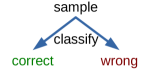
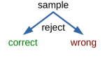
Performance on known classes (clean, corrupt, and adversarial samples) is typically evaluated by calculating the classification accuracy (or equivalently the percentage error), see Fig. 2 and Table 1, although many other metrics can also be used (Guo et al., 2023). However, if models are to be allowed to reject samples, to deal with those from unknown classes, then the performance on known samples should also be assessed taking into account that some samples may be rejected. On the other hand, models designed to perform unknown class rejection (Kirchheim et al., 2022; Chen et al., 2023; Cheng et al., 2023; Xu-Darme et al., 2023; Yang et al., 2022, 2023; Lee et al., 2022), and adversarial defences that reject perturbed samples (Stutz et al., 2020; Ren et al., 2022; Lee et al., 2022; Chen et al., 2022), are typically evaluated purely in terms of how accurately samples are rejected and accepted. In other words, the task is considered to be that of binary classification (see Fig. 2 and Table 1). Hence, standard metrics for binary classification can be used, such as the False Positive Rate when the true positive rate is X% (FPR@X%), which assesses performance for a single rejection threshold, or Area Under the Receiver Operating Characteristic curve (AUROC) or Area Under the Precision-Recall curve (AUPR) both of which assess performance over varying rejection thresholds. An issue with FPR@X% is that separate thresholds are used for distinguishing each unknown data-set from the clean test data. Worse still, some rejection methods have hyper-parameters that are tuned separately on each unknown data-set (Zhang et al., 2023). This is unrealistic, as in the real-world a single rejection criteria with fixed hyper-parameters would need to work to reject any unknown data, regardless of its origin (Shafaei et al., 2018; Feng et al., 2022). An issue with all standard unknown class rejection metrics is that the ability of the model to accurately classify the accepted samples is not evaluated. In some publications the clean accuracy of the model is evaluated, but this is done without any samples being rejected, and hence, does not reflect the performance that would be expected in the real-world where the same rejection criteria would be applied to all samples.

Figure 2: Decision trees illustrating standard assessment methods for (a) known class data, and (b) unknown class rejection. (c) The method proposed by Zhu et al. (2022).

Table 1: Confusion matrices illustrating assessment methods for (a) known class data, (b) unknown class rejection, and (c) the method proposed by Zhu et al. (2022). For (a) performance is typically evaluated by calculating the proportion of correct predictions. For (b) performance is typically evaluated by calculating the $\mathrm{FPR}=\frac{\mathrm{FP}}{\mathrm{FP}+\mathrm{TN}}$ when the rejection threshold has been set to produce a predetermined $\mathrm{TPR}=\frac{\mathrm{TP}}{\mathrm{TP}+\mathrm{FN}}$, where $\mathrm{TP}$, $\mathrm{FN}$, $\mathrm{FP}$, and $\mathrm{TN}$ are the total number of true-positives, false-negatives, false-positives, and true-negatives, respectively. (c) Considers both if the sample has been correctly accepted or rejected, and whether the predicted class label is correct or incorrect.

		predicted class
		1	2	…	c
true class	1	✓	✗		✗
	2	✗	✓		✗
	⋮
	c	✗	✗		✓

		predicted
		accept	reject
true	known	$\mathrm{TP}$	$\mathrm{FN}$
	unknown	$\mathrm{FP}$	$\mathrm{TN}$

				predicted class
				correct	wrong
true	known	predicted	accept	$\mathrm{TP}$	$\mathrm{FP}$
			reject	$\mathrm{FN}$	$\mathrm{TN}$
	unknown		accept	N/A	$\mathrm{FP}$
			reject	N/A	$\mathrm{TN}$

Some metrics do attempt to evaluate classification performance in the presence of rejection. For example, in the context of evaluating accuracy on adversarial data, confidence-thresholded robust error (Stutz et al., 2020) measures the classification error for test examples that are not rejected, when the rejection threshold has been set so that 1% of correctly classified clean examples can be rejected. Using the metric robust risk with detection (Tramèr, 2021) a classifier is accurate if it correctly classifies the clean samples, and either rejects or correctly classifies perturbed samples. However, with these metrics a high score can be obtained by a classifier that rejects a large proportion of the perturbed samples, even though these samples come from a known class and may be only perturbed imperceptibly (Chen et al., 2022). To address this issue, robustness with rejection (Chen et al., 2022) defines a variable perturbation threshold that can vary from zero to the adversarial attack budget. For test samples with a perturbation less than or equal to the threshold, both incorrect classification and rejection is counted as an error. For test samples with a perturbation greater than the threshold, incorrect classification is considered an error, but rejection is not counted as an error. When the threshold is greater or equal to the attack perturbation budget, robustness with rejection is equivalent to standard robust error. When the threshold is zero this metric is equivalent to robust risk with detection as proposed by Tramèr (2021).

An issue with all the methods discussed in the previous paragraph, is that they define which samples can be rejected in terms of an arbitrary measure of distribution shift in the input space (Guérin et al., 2023). This means that these methods would not allow for rejection of non-adversarial samples. For example, in the situation where the sample is clean but ambiguous (e.g., in an optical character recognition task a letter written in terrible handwriting) rejection would be counted as an error even though the distribution shift for such a sample might be far higher than that of any adversarial sample. These metrics would also be incapable of assessing performance on data-sets containing unknown samples. In this situation the correct action of the classifier is to reject all samples, however, for confidence-thresholded robust error (Stutz et al., 2020) a score is only calculated for accepted samples, so no score could be calculated for a classifier correctly rejecting all unknown samples. Both robustness with rejection (Chen et al., 2022) and robust risk with detection (Tramèr, 2021) would suffer from the same issue, assuming unknown samples were considered to be sufficiently perturbed to be out-of-distribution. Alternatively, if clean samples from unknown classes were considered to be unperturbed, these metrics would give a score of zero to a classifier that correctly rejected all samples, as any rejection of clean sample is counted as an error for these metrics.

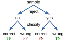
It would be more reasonable to decide whether or not rejection or acceptance of the sample was the correct choice depending on whether or not that sample would have been mis-classified or correctly classified (Pang et al., 2022), as the goal of sample rejection is to protect the classifier from making predictions that are unreliable, not to identify samples that differ from the training data (Guérin et al., 2023; Zhu et al., 2022). Taking this approach, Zhu et al. (2022) propose a metric that they apply to evaluate the performance of classifiers using both corrupt samples and unknown samples from novel classes. As shown in Fig. 2 and Table 1, unlike standard metrics, this approach considers both whether or not a sample is rejected, and whether or not the classification label predicted by the classifier is correct. In this scheme, a sample is considered a true-positive ($\mathrm{TP}$) if it is not rejected and assigned the correct class label. A sample is a false-positive ($\mathrm{FP}$) if it is accepted but incorrectly classified. A false-negative ($\mathrm{FN}$) is a sample that is rejected although it would have been assigned the correct class label. Finally, true-negatives ($\mathrm{TN}$) are samples that are rejected and that would have been classified incorrectly. The proposed metric is the detection error rate (DER), which counts the number of false positives and false-negatives as a proportion of all test samples. Zhu et al. (2022) apply their metric using two rejection thresholds, that are set such that either 95% or 99% of correctly classified clean examples are accepted. These different values for the rejection threshold define the trade-off between accuracy on the clean data (perfect performance on the clean data could only be achieved if 100% of correctly classified clean examples were accepted) and correct rejection of unknown samples (good performance on unknown class rejection is more likely if more clean samples are also rejected).

2 Methods

2.1 Proposed Assessment Method

This article proposes to extend and modify the evaluation method proposed by Zhu et al. (2022), described in the preceding section, in the following ways:

1. Measuring performance in terms of accuracy rather than error. The metric defined by Zhu et al. (2022), DER, is a measure of the proportion of errors (express as a percentage) made by the classifier. Here, the percentage of correctly processed samples is reported. This simple change means that a higher score correlates with improved performance which is more intuitive, and is more consistent with previously used metrics (such a AUROC and those used in RobustBench (Croce et al., 2021)) where this is also the case. Hence, rather than using detection error rate (DER), detection accuracy rate (DAR) is reported.

2. Summarising results by averaging over task, not data-set. Zhu et al. (2022) report results for each data-set separately. However, using many separate metrics makes it difficult to evaluate the overall robustness of any model especially when there are trade-offs in performance of different data-sets (meaning that no method of improving robustness is likely to have strong performance across all data-sets). It is therefore convenient to have a single metric to summarise performance. For this purpose, Zhu et al. (2022) average the performance across each data-set. However, there is a risk that a more extensive evaluation of robustness using more data-sets might result in this average becoming biased towards one type of robustness. For example, as there are potentially a very large number of data-sets containing images from unknown classes, including more such data-sets would result in the average performance favouring methods better able to reject unknown classes. Alternatively, calculating a single value of the metric using all data from all data-sets would be biased towards favouring methods better able to deal with data-sets containing the most samples. To better balance the importance of robustness to each type of data, here a single summary metric is obtained by calculating the metrics separately for each type of data, and then averaging across data type .

3. Extending the evaluation to consider other forms of generalisation. Zhu et al. (2022) evaluate performance using several data-sets including clean and corrupt data and data from unknown classes. In the current work, unknown class rejection is evaluated not only using images from novel classes, as in (Zhu et al., 2022), but also using unrecognisable images. Furthermore, performance is also evaluated using adversarial samples. In other words, here performance is evaluated using the five types of data illustrated in Fig. 1, whereas Zhu et al. (2022) use only three.

2.2 Choice of Test Data

The current work tested the performance of Deep Neural Networks (DNNs) trained on the following data-sets: CIFAR10, CIFAR100, TinyImageNet, and MNIST. In each case training was performed with the standard training sub-set of data. The robustness of each trained network was tested using the five categories of test data illustrated in Fig. 1. Within each category the following data was used.

Clean.

The standard test-set provided with each data-set.

Corrupt.

Popular common corruptions data-sets were used: CIFAR10-C, CIFAR100-C, TinyImageNet-C and MNIST-C (Hendrycks and Dietterich, 2019; Mu and Gilmer, 2019). The first three data-sets contain 18 different corruptions including different types of noise, blurring, synthetic weather conditions, and digital corruptions. MNIST-C contains 15 different corruptions including different types of noise, blurring, geometric transformations, and superimposed patterns. As typical in the literature, performance was evaluated using all the corruptions at all degrees of intensity.

Adversarial.

Samples were produced using AutoAttack (AA; Croce and Hein, 2020), a state-of-the-art ensemble attack method that employs both gradient-based (white-box) and gradient-free (black-box) attacks. AA was implemented using the torchattacks PyTorch library (Kim, 2021). Two sets of adversarial samples where created. Each set was created by perturbing the entire standard (clean) test-set, but with a different method of constraining the magnitude of the perturbation. Specifically, AA was used to apply both $l_{\infty}$ and $l_{2}$-norm constrained attacks. The perturbation budget ($\epsilon$) used for each attack was the standard value used in the previous literature for each data-set. Specifically, $\epsilon$ was set to $\frac{8}{255}$ and 0.5 for $l_{\infty}$ and $l_{2}$-norm attacks, respectively, against networks trained on the CIFAR10, CIFAR100, and TinyImageNet data-sets, and $\epsilon$ was set to 0.3 for $l_{\infty}$-norm and to 2 for $l_{2}$-norm attacks on MNIST trained networks.

Novel Class.

In each case, three data-sets containing objects of unknown classes were chosen. Specifically, the CIFAR10 and CIFAR100 trained networks were tested using novel classes from the test-sets of the Textures (Cimpoi et al., 2014) and SVHN (Netzer et al., 2011) data-sets and the CIFAR data-set that was not used for training (i.e., a CIFAR10 trained network was evaluated on its ability to reject samples from CIFAR100, and vice versa). For TinyImageNet trained networks novel class data came from the Textures test set (Cimpoi et al., 2014), the iNaturalist 2021 validation set (Horn et al., 2018), and the ImageNet-O data-set (Hendrycks et al., 2019b). The MNIST trained networks were tested using unknown, novel, classes from the test-sets of the Omniglot (Lake et al., 2015), FashionMNIST (Xiao et al., 2017) and KMNIST (Clanuwat et al., 2018) data-sets.

Unrecognisable.

Data to test unrecognisable image rejection was the same for all networks, and consisted of synthetic images randomly generated using four different methods. First, images containing random blobs, as used in (Hendrycks et al., 2019c). Secondly, images in which each pixel intensity value was independently and randomly selected from a uniform distribution. Thirdly, the images of the standard (clean) test set after a random permutation of all pixels. Fourthly, the images of the clean test set after randomising the phase, in the Fourier domain, of each image. Each of these four data-sets contained the same number of samples as the standard test-set associated with the training data.

In principal, the amount of test data that could be used is unlimited (as there are countless images containing objects that any one classifier has not been trained to recognise, and due to the stochastic nature of the methods used to create corrupt, adversarial, and unrecognisable images). Hence, the above selection of test data necessarily represents a small, arbitrary, sub-set of all the possible data that could be used. In making this selection the aim was to define a reasonably wide variety of data while ensuring that evaluation could be performed in a reasonable time using reasonable resources. The results in Section 3 suggest that the chosen data is sufficiently challenging that modern DNNs are far from ceiling performance. However, as classification methods improve in the future, the data used for evaluation could be extended to allow a more thorough and challenging assessment in two ways: adding more data in each category, or by adding categories.

Expanding the range of data in each of the existing categories could be done by: using new sets of clean data (such as CIFAR10.1 (Recht et al., 2018), or ImageNet-A (Hendrycks et al., 2021a)); using different corruptions (e.g., different forms of noise or image transformation), higher magnitude corruptions (e.g., a wider range of scales such as used in the MNIST Large Scale data set (Jansson and Lindeberg, 2020)), objects shown against different backgrounds (as is used in the NICO challenge (Zhang et al., 2023)); using any of numerous alternative algorithms for generating adversarial images (Liang et al., 2022; Ren et al., 2020; Xu et al., 2020), or different methods of constraining the perturbations, or higher perturbation budgets; using the additional novel class data-sets proposed in the OpenOOD benchmark Yang et al. (2022); using fooling images (Kumano et al., 2022; Nguyen et al., 2015) that are unrecognisable images which have been optimised to be difficult to reject. Adversarial attack-type techniques could also be used not only to perturb clean test samples, as is currently the case, but samples from other data types to make these types of data more challenging to correctly process. New categories of test data that could be used to extend and increase the challenge of the proposed benchmark include: known classes presented in the form of drawings, art, or cartoons (such as in ImageNet-R (Hendrycks and Dietterich, 2019) or PACS (Li et al., 2017)); or images where texture has been replaced by that from another image (Geirhos et al., 2019).

2.3 Rejection Criteria

In order for classifiers to be evaluated using the proposed method, it is necessary to define a criteria that will be used to determine if a sample is accepted for classification, or rejected. Many different methods for unknown class rejection have been proposed (Vaze et al., 2022; Pang et al., 2022; Chen et al., 2022; Hendrycks and Gimpel, 2017; Tajwar et al., 2021). This article will primarily use maximum softmax probability (MSP; Hendrycks and Gimpel, 2017), which defines the confidence that a sample is of a known class as the maximum response of the network output after application of the softmax activation function. MSP is used as this is a standard, baseline method, used frequently in the literature on unknown class rejection. Furthermore, a comparison of different rejection methods using the same metric on which the proposed benchmark is based found MSP to be one of the best methods (Zhu et al., 2022).

Previous work has shown that relative performance of different unknown class rejection methods vary depending on the data-sets Tajwar et al. (2021) and models (Zhu et al., 2022) used. Hence, to confirm that the results obtained in this study are not unique to MSP results for three other post-hoc methods of unknown class rejection (those that rely on the responses produced by the network) are also reported. (1) Maximum logit score (MLS; Vaze et al., 2022), which defines the confidence that a sample is of a known class as the maximum response of the network output before any activation function is applied. This was shown to be the best method of unknown class rejection in a recent comparison of state-of-the-art methods (Vojir et al., 2023). (2) Energy score (Liu et al., 2020), which defines confidence as the negative logarithm of the denominator of the softmax activation function applied the network output layer. (3) GEN (Liu et al., 2023) a very recently proposed method that claims to be superior to all three other methods considered here.

Consistent with the method proposed by Zhu et al. (2022), a rejection threshold is set such that a fixed percentage correctly classified clean examples are accepted. In other words, such that the confidence associated with those samples (calculated using either MSP, MLS, Energy score or GEN depending on the experiment being performed), is greater than or equal to the threshold. All samples, from any data-set, with confidence lower than the threshold are rejected, while all others are accepted and the class label predicted.

2.4 Choice of Models to Assess

The aim of the current work is to determine how well existing DNNs perform when evaluated using the more comprehensive assessment methods advocated above. However, it is clearly impossible to attempt to evaluate the performance of every network architecture or to evaluate the huge variety of different techniques that has been proposed for improving adversarial robustness, generalisation to common corruptions, or for unknown class rejection.

ResNet18 (He et al., 2016) was chosen as the principal DNN architecture to test as this is very commonly used in the literature. This model has just over 11M trainable parameters. Additional experiments were also performed using WideResNet34-20 (Zagoruyko and Komodakis, 2016) which has just under 193M parameters. For the MNIST data-set smaller networks were used. Firstly, a full-connected multi-layer perceptron network, containing 200 neurons in each of 3 hidden layers (denoted as MLP200-200-200). This network used the ReLU activation function and had 239,410 trainable parameters. Secondly, a fully-convolutional neural network (ConvNet) containing 5 layers, with 32 3x3 convolutional filters in each hidden layer, and average pooling of stride 2 applied after the first and second layers. The ReLU activation function was applied to each layer (except the final output). This network is denoted as ConvNet5-3-32 where the numbers indicate the depth, kernel-size, and width respectively. This network contained 30,954 trainable parameters.

A common approach to improving performance on all the different types of test-data described in Section 1.2 is to use data augmentation techniques: i.e., to expand the training data-set by creating new samples that are synthetically manipulated versions of samples from the original training data-set. In the results section (Section 3) a number of such techniques are evaluated. The selection of the particular methods to test was made so as to include standard baselines and state-of-the-art methods for producing robust models for all the different types of test-data described in Section 1.2.

baseline

Improved performance on the standard test data is often achieved by applying simple geometric data augmentations to the training data. Here 4-pixel random cropping and random horizontal flipping where applied to the CIFAR10, CIFAR100 and TinyImageNet training data, while no augmentations were applied to the MNIST data. These standard augmentations were used in combination with the additional augmentation methods listed below. Given that these baseline augmentation methods are very commonly used when training models, the results show how standardly trained networks cope under comprehensive evaluation. The results for this method of training also provides a baseline against which to judge the effectiveness of other methods that have been proposed to improve generalisation performance.

noise

Augmenting training images with random noise has been shown to reduce over-fitting, and hence, improve generalisation (Sietsma and Dow, 1991; Holmstrom and Koistinen, 1992; Goodfellow et al., 2016), especially to common image corruptions (Rusak et al., 2020; Ford et al., 2019). Various methods of adding noise to the training data have been proposed. Rusak et al. (2020) augmented half the training data with Gaussian noise, and found that this technique produced performance on corrupt test data that was competitive with the more complex augmentation method, AugMix, and that for the MNIST data-set specifically was just as effective as their proposed method of Adversarial Noise Training. Lopes et al. (2019) advocated adding Gaussian noise to only a randomly chosen patch of the image, which they claimed produced better robustness to image corruptions on CIFAR10 data than applying random noise to the whole image. Ford et al. (2019) used an alternative method for corrupting training images with Gaussian noise in which the standard deviation of the noise applied to each image was chosen with equal probability from the range $[0,\sigma_{u}]$. The method implemented here is a generalisation for the method proposed by Ford et al. (2019). Specifically, for each image the standard deviation of the noise was chosen from a uniform distribution with range $[\sigma_{l},\sigma_{u}]$. Then each pixel intensity value was independently modified by the addition of a value chosen at random from a Gaussian distribution with mean of zero and the chosen standard deviation. The original images had pixel intensity values in the range [0,1], and after the application of the noise pixel values were clipped at 0 and 1 to remain in this range. Appropriate values of $\sigma_{l}$ and $\sigma_{u}$ were found via a grid search using small ConvNets. Using this method $\sigma_{l}=0$ and $\sigma_{u}=0.4$ were chosen for use with CIFAR10, and the same hyper-parameters were also used for CIFAR100 and TinyImageNet. For MNIST $\sigma_{l}=\sigma_{u}=0.5$ was used.

AT

Multi-step adversarial training with Projected Gradient Descent (PGD; Madry et al., 2018) is a standard, and highly effective, defence against adversarial attack. As a result, this method has become a standard benchmark against which all other methods of adversarial defence are judged. This method was, therefore, also selected as a data augmentation technique to be tested. It was implemented using the torchattacks PyTorch library (Kim, 2021). To perform adversarial training, clean images from the current batch of training examples were used to generate non-targeted adversarial examples, that then replaced the original training images (as in Madry et al., 2018). Following standard protocols, the maximum allowed perturbation was constrained by the $l_{\infty}$-norm to be less than the perturbation budget ($\epsilon$), and the training-time adversarial images were generated using 10 steps of PGD (denoted as PGD${}_{l_{\infty}}^{10}$ for brevity). Standard values used in the previous literature were used for $\epsilon$. Specifically, $\epsilon$ was set to $\frac{8}{255}$ for performing AT with the CIFAR10, CIFAR100 and TinyImageNet training data, and $\epsilon=0.3$ was used for MNIST.

pixmix

This is a training data augmentation pipeline that repeatedly mixes (either additively or multiplicatively) an augmented image with an augmented clean image or a fractal image (Hendrycks et al., 2022). It is claimed that this augmentation method can improve generalisation to both clean and corrupt data, improve adversarial robustness, and improve unknown class rejection. This method of data augmentation was therefore also tested using the proposed, comprehensive, evaluation method. It was implemented using the official code released by the original authors.

regmixup

This is a variation on mixup (Zhang et al., 2017) that is specifically designed to improve performance on both corrupt data and on unknown class rejection (Pinto et al., 2023). It was re-implemented with custom code.

In addition, evaluations were also performed on current state-of-the-art robust pre-trained models available from the RobustBench model zoo (Croce et al., 2021).

2.5 Experimental Setup

Training was performed using a batch size of 128. For the CIFAR10, CIFAR100 and TinyImageNet data-sets, training was performed for 110 epochs using the SGD optimiser with weight decay of 5e-4 and an initial learning rate of 0.1. The learning rate was step-wise decayed by a factor of 10 at the start of epochs 100 and 105 for the CIFAR data-sets, and at epochs 45 and 89 for TinyImageNet. The set-up for the CIFAR data-sets was based on that recommended for AT by Pang et al. (2021). Hence, these hyper-parameters may not be optimal for training with the other data augmentations used. For the MNIST data, 20 epochs of training using the Adam optimiser and a constant learning rate of 0.001 was used.

For each experimental condition (combination of data-set, network architecture, and training data augmentation method) the network was trained and evaluated three times, each time with a different random weight initialisation and random presentation order of training samples. The reported result for each condition is the mean accuracy over these three trials. The standard-deviation in the mean performance measured using the proposed metric is shown in the tables of results and generally shows a high degree of consistency across trials. Exceptions to the above, where only a single trial was performed, were the experiments with WideResNet34-20 and the experiments performed using a publicly available checkpoint created by other researchers.

3 Results

3.1 Comparison with Standard Metrics

Table 2: Performance of different methods for improving generalisation applied to CIFAR10 trained ResNet18 networks when MSP is used as the rejection criteria. Sub-tables show performance measured using (a) standard metrics, and the proposed metric, DAR, when the rejection threshold is set to accept (b) 99% or (c) 95% of correctly classified clean examples.

Training	Clean	Corrupt	AA${}_{l_{\infty}}$	AA${}_{l_{2}}$	Textures	SVHN	CIFAR100	Phase	Scramble	Blobs	Uniform
Method	Accuracy (%)				AUROC (%)
baseline	$94.46$	$74.59$	$0.00$	$0.02$	$91.60$	$95.99$	$89.05$	$95.54$	$92.64$	$94.86$	$87.57$
noise	$88.73$	$82.29$	$4.10$	$38.01$	$88.45$	$89.67$	$83.90$	$88.67$	$75.51$	$91.25$	$98.86$
AT	$83.91$	$75.68$	[rm]bfb$48.80$	[rm]bfb$59.35$	$83.82$	$88.38$	$77.36$	$77.72$	$59.16$	$71.46$	$83.02$
pixmix	$94.10$	[rm]bfb$88.32$	$0.00$	$1.26$	[rm]bfb$98.89$	[rm]bfb$98.48$	[rm]bfb$91.74$	[rm]bfb$99.38$	[rm]bfb$99.82$	[rm]bfb$99.96$	[rm]bfb$99.85$
regmixup	[rm]bfb$94.67$	$80.43$	$0.00$	$0.00$	$92.05$	$94.26$	$88.81$	$95.32$	$98.33$	$95.21$	$99.78$

(a) Existing Metrics

Training Method	Clean	Corrupt	Adversarial	Novel	Unrecog.	Mean $\pm$ Std
baseline	$94.66$	$78.85$	$1.18$	$38.97$	$26.63$	$48.06\pm 0.00$.77)
noise	$89.50$	$84.12$	$23.16$	$20.08$	$37.68$	$50.91\pm 0.00$.99)
AT	$84.80$	$77.84$	[rm]bfb$58.29$	$17.35$	$2.22$	$48.10\pm 0.00$.17)
pixmix	$94.35$	[rm]bfb$88.97$	$2.14$	[rm]bfb$73.33$	[rm]bfb$97.23$	[rm]bfb$71.20\pm 0.00$.13)
regmixup	[rm]bfb$94.95$	$84.15$	$1.92$	$32.94$	$67.61$	$56.31\pm 0.00$.87)

(b) DAR (%) @ 99% clean data acceptance

Training Method	Clean	Corrupt	Adversarial	Novel	Unrecog.	Mean $\pm$ Std
baseline	$93.20$	$80.92$	$3.57$	$74.61$	$62.62$	$62.98\pm 0.03$.30)
noise	$89.24$	$84.94$	$29.60$	$51.93$	$56.28$	$62.40\pm 0.00$.30)
AT	$85.50$	$80.26$	[rm]bfb$68.55$	$49.76$	$13.31$	$59.48\pm 0.01$.28)
pixmix	$92.91$	$85.36$	$5.59$	[rm]bfb$87.98$	[rm]bfb$99.73$	[rm]bfb$74.31\pm 0.00$.13)
regmixup	[rm]bfb$93.26$	$82.16$	$14.77$	$69.41$	$89.99$	$69.92\pm 0.00$.90)

(c) DAR (%) @ 95% clean data acceptance

Table 3: Results equivalent to those shown in Table 2 for networks trained on CIFAR100.

Training Method	Clean	Corrupt	AA${}_{l_{\infty}}$	AA${}_{l_{2}}$	Textures	SVHN	CIFAR10	Phase	Scramble	Blobs	Uniform
	Accuracy (%)				AUROC (%)
baseline	[rm]bfb$76.66$	$49.68$	$0.00$	$0.04$	$77.08$	$79.11$	$76.20$	$79.00$	$70.82$	$82.17$	$93.60$
noise	$65.19$	$57.31$	$2.70$	$20.97$	$66.63$	$80.79$	$70.64$	$81.67$	$44.70$	$81.83$	$94.41$
AT	$57.45$	$47.33$	[rm]bfb$25.40$	[rm]bfb$34.77$	$65.69$	$78.69$	$67.22$	$62.67$	$27.47$	$58.69$	$16.27$
pixmix	$73.70$	[rm]bfb$62.88$	$0.00$	$0.56$	[rm]bfb$88.31$	[rm]bfb$88.02$	$74.08$	[rm]bfb$93.42$	[rm]bfb$99.53$	[rm]bfb$99.66$	[rm]bfb$99.94$
regmixup	$76.27$	$53.51$	$0.00$	$0.07$	$77.11$	$81.26$	$77.61$	$83.56$	$65.63$	$79.25$	$73.74$

(d) Existing Metrics

Training Method	Clean	Corrupt	Adversarial	Novel	Unrecog.	Mean $\pm$ Std
baseline	[rm]bfb$78.63$	$57.34$	$2.90$	$18.47$	$19.52$	$35.37\pm 0.02$.73)
noise	$68.09$	$62.46$	$15.98$	$17.83$	$18.29$	$36.53\pm 0.01$.45)
AT	$60.88$	$52.98$	[rm]bfb$36.14$	$14.89$	$0.57$	$33.09\pm 0.00$.49)
pixmix	$75.91$	[rm]bfb$69.01$	$3.93$	[rm]bfb$32.09$	[rm]bfb$88.17$	[rm]bfb$53.82\pm 0.01$.65)
regmixup	$78.51$	$59.84$	$3.42$	$14.57$	$6.76$	$32.62\pm 0.00$.28)

(e) DAR (%) @ 99% clean data acceptance

Training Method	Clean	Corrupt	Adversarial	Novel	Unrecog.	Mean $\pm$ Std
baseline	[rm]bfb$81.69$	$67.57$	$9.23$	$42.43$	$49.76$	$50.14\pm 0.01$.76)
noise	$74.06$	$70.90$	$26.52$	$46.74$	$53.47$	$54.34\pm 0.01$.09)
AT	$66.90$	$62.45$	[rm]bfb$48.94$	$39.00$	$4.31$	$44.32\pm 0.00$.38)
pixmix	$79.87$	[rm]bfb$75.20$	$11.28$	[rm]bfb$60.99$	[rm]bfb$95.67$	[rm]bfb$64.60\pm 0.01$.19)
regmixup	$81.25$	$69.53$	$10.09$	$43.43$	$28.98$	$46.66\pm 0.00$.97)

(f) DAR (%) @ 95% clean data acceptance

Table 2 shows results for ResNet18 networks trained on CIFAR10 using different training-time data augmentation methods that have been proposed to improve performance (as discuss in Section 2.4). Table 3 shows equivalent results for CIFAR100 trained networks. Evaluation of the performance of these networks using standard metrics is shown in Figs. 3(a) and 3(d). It can be seen that, as expected, AT with PGD${}_{l_{\infty}}^{10}$ produces the best defence against adversarial attacks with AA. It can also be seen that, compared to a network trained with the baseline augmentations, AT causes a reduction in the accuracy with which clean data is categorised and a reduction in performance on unknown class rejection. Also not unexpectedly, pixmix produces the best performance on unknown class rejection for all the data-sets (except CIFAR10 for the CIFAR100 trained network), and produces the best performance on the corrupt data.

These findings are also captured by the new evaluation metric, results for which are shown in Figs. 3(b) and 3(e) when the rejection threshold is set such that 99% of correctly classified clean examples are accepted. The results summarising performance on each type of data show that AT produces the highest accuracy for adversarial samples, and pixmix produces the highest accuracy on corrupt data and the two types of unknown class data (novel and unrecognisable). The trade-offs in performance over different types of data can also be seen. The average performance over all data types (shown in the last columns of each table) suggests that pixmix produces the best performance overall.

The results for all methods on unknown class data is far worse than the standard metrics would imply. This is because the same rejection threshold has been used for all data types, rather than being tuned to optimise performance on unknown class rejection. This illustrates that current metrics for unknown class rejection grossly over-estimate likely real-world performance (as discussed in Section 1.5). In contrast, the performance of all methods on known class data (clean, corrupt and adversarial) is higher than would be expected from the standard metrics. This is because networks can reject samples for which prediction confidence is low which include many samples for which the predicted class is wrong.

Note that these results generally show that current methods of training deep networks produce classifiers that lack robustness. For most of the methods evaluated (which includes methods that are designed to produce state-of-the-art robustness) the resulting network can only make the correct decision on around 50% of the samples for CIFAR10, which is a relatively simple data-set. Even pixmix, that performs best overall, only makes accurate decisions for just over 71% of the test data. Furthermore, it might reasonably be argued that a model is only as robust as the worst results would suggest, as a malicious actor can select the type of data used to attack a system, and in the real world a model might naturally encounter all types of data and would need to deal correctly with all. For each method of training investigated here there is at least one type of test data on which the model performs pitifully. For example, AT can only correctly reject 2.2% of unrecognisable images: all the others are given incorrect class labels with a high confidence. Massive amounts of time and resources have gone into developing techniques to enhance adversarial robustness. The current results suggest that this effort may have been wasted, as an attacker can easily and effectively induce a classifier to generate the wrong predictions by presenting it with easily generated synthetic images. The results in Section 3.5 show that the most recent state-of-the-art methods of adversarial robustness, while having better performance on unknown class rejection, are still far from robust to such data.

Figs. 3(c) and 3(f) show results for the proposed evaluation method when the rejection threshold is set such that 95% of correctly classified clean examples are accepted (an increased rejection threshold compared to previously). For the CIFAR10 trained networks, rejecting more of the clean samples results in a reduction in performance on the clean data as some samples that were correctly classified have been rejected. In contrast, the results for CIFAR100 show that performance on the clean data improves with the increased rejection threshold, due to the higher proportion of clean samples that are mis-classified by the CIFAR100 trained networks. For both data-sets, rejecting more samples for which confidence in the prediction is low results in a large improvement in performance on the adversarial, novel and unrecognisable data types for all training methods.

The results produced with both thresholds are consistent showing similar trade-offs in performance on the different data types for each of the tested methods, and producing similar rankings of different training methods, although the differences between methods is somewhat reduced when the threshold is set so as to accept 95% of correctly classified clean samples. To avoid redundancy, and for brevity, only results for one threshold are reported subsequently. The 95% threshold was chosen in order to present the most favourable performance for the tested DNNs.

3.2 Different Unknown Class Rejection Methods

Table 4: Results equivalent to those shown in Fig. 3(c) but for different rejection criteria.

	Training Method	Clean	Corrupt	Adversarial	Novel	Unrecog.	Mean $\pm$ Std
MLS	baseline	$92.50$	$79.65$	$2.88$	$81.35$	$77.74$	$66.82\pm 0.04$.33)
	noise	$88.41$	$84.01$	$27.40$	$56.13$	$66.05$	$64.40\pm 0.00$.59)
	AT	$84.36$	$79.01$	[rm]bfb$65.87$	$52.56$	$14.95$	$59.35\pm 0.02$.31)
	pixmix	$92.02$	$82.35$	$4.10$	[rm]bfb$90.26$	[rm]bfb$99.97$	[rm]bfb$73.74\pm 0.00$.07)
	regmixup	[rm]bfb$92.58$	$80.02$	$4.19$	$67.67$	$93.77$	$67.65\pm 0.01$.83)
Energy	baseline	[rm]bfb$92.34$	$79.23$	$2.73$	$81.01$	$78.25$	$66.71\pm 0.04$.59)
	noise	$87.96$	[rm]bfb$83.29$	$26.96$	$52.84$	$67.49$	$63.71\pm 0.00$.72)
	AT	$83.33$	$77.15$	[rm]bfb$63.44$	$44.40$	$12.54$	$56.17\pm 0.01$.87)
	pixmix	$91.79$	$81.71$	$3.80$	[rm]bfb$90.09$	[rm]bfb$99.98$	[rm]bfb$73.47\pm 0.00$.08)
	regmixup	$92.09$	$78.78$	$3.27$	$59.88$	$91.92$	$65.19\pm 0.02$.20)
GEN	baseline	[rm]bfb$92.55$	$79.82$	$2.93$	$81.64$	$77.60$	$66.91\pm 0.04$.33)
	noise	$88.13$	$83.63$	$27.08$	$54.65$	$66.87$	$64.07\pm 0.00$.65)
	AT	$83.49$	$77.45$	[rm]bfb$63.80$	$46.67$	$12.56$	$56.79\pm 0.01$.80)
	pixmix	$91.93$	$82.08$	$3.94$	[rm]bfb$90.19$	[rm]bfb$99.97$	[rm]bfb$73.62\pm 0.00$.08)
	regmixup	$92.26$	$79.33$	$3.73$	$64.71$	$93.09$	$66.62\pm 0.02$.15)

Table 5: Results equivalent to those shown in Fig. 3(f) but for different rejection criteria.

	Training Method	Clean	Corrupt	Adversarial	Novel	Unrecog.	Mean $\pm$ Std
MLS	baseline	[rm]bfb$80.00$	$67.31$	$7.59$	$55.63$	$54.70$	$53.05\pm 0.02$.19)
	noise	$72.74$	$70.20$	$24.91$	$52.15$	$55.03$	$55.00\pm 0.00$.95)
	AT	$66.00$	$62.34$	[rm]bfb$47.55$	$41.10$	$3.11$	$44.02\pm 0.00$.21)
	pixmix	$78.49$	$73.72$	$9.96$	[rm]bfb$68.39$	[rm]bfb$97.66$	[rm]bfb$65.64\pm 0.00$.86)
	regmixup	$80.42$	$68.21$	$9.01$	$37.02$	$24.93$	$43.92\pm 0.00$.34)
Energy	baseline	[rm]bfb$79.33$	$66.16$	$6.96$	$56.80$	$53.34$	$52.52\pm 0.01$.95)
	noise	$71.45$	$68.72$	$23.50$	$50.58$	$51.98$	$53.25\pm 0.01$.16)
	AT	$63.50$	$60.24$	[rm]bfb$43.70$	$40.32$	$2.81$	$42.11\pm 0.00$.32)
	pixmix	$77.24$	$72.12$	$8.73$	[rm]bfb$68.28$	[rm]bfb$97.87$	[rm]bfb$64.85\pm 0.00$.78)
	regmixup	$78.56$	$64.23$	$6.96$	$23.60$	$19.32$	$38.54\pm 0.02$.12)
GEN	baseline	[rm]bfb$79.47$	$66.45$	$7.09$	$56.59$	$53.52$	$52.63\pm 0.02$.14)
	noise	$71.60$	$68.96$	$23.65$	$50.88$	$52.38$	$53.49\pm 0.01$.05)
	AT	$63.66$	$60.35$	[rm]bfb$43.94$	$40.24$	$2.73$	$42.18\pm 0.00$.36)
	pixmix	$77.38$	$72.29$	$8.87$	[rm]bfb$68.19$	[rm]bfb$97.77$	[rm]bfb$64.90\pm 0.00$.87)
	regmixup	$78.76$	$64.80$	$7.19$	$25.80$	$19.92$	$39.30\pm 0.01$.76)

The same networks evaluated in the previous section were re-evaluated using MLS, Energy score and GEN as the criteria for rejection (see Section 2.3). The results for the networks trained on CIFAR10 are shown in Table 4, and for CIFAR100 in Table 5. Comparing the results in Table 4 with the results obtained using MSP shown in Fig. 3(c) it can be seen that while individual accuracy values can vary, a similar overall performance is produced using each method of rejection, and as a result a similar ranking of the overall performance of each training method is obtained. The same can be said for the CIFAR100 results shown in Table 5 and Fig. 3(f). The results obtained, therefore, do not seem to be specific to the particular method of rejection used, and to avoid redundancy, and for brevity, only results for MSP are reported subsequently. This choice was made as the worse performance on any data type is better for MSP than for any of the other three methods, and hence, MSP seems to have a slight advantage in improving robustness.

3.3 Effects of Increasing Network Capacity

Table 6: Results equivalent to those shown in Fig. 3(c) but for WideResNet34-20.

Training Method	Clean	Corrupt	Adversarial	Novel	Unrecog.	Mean
baseline	[rm]bfb$93.96$	$81.79$	$3.29$	$78.47$	$80.43$	$67.59$
noise	$91.74$	[rm]bfb$87.40$	$33.68$	$55.38$	$56.89$	$65.02$
AT	$87.59$	$82.10$	[rm]bfb$72.74$	$46.32$	$33.02$	$64.36$
pixmix	$93.90$	$87.18$	$6.56$	[rm]bfb$89.08$	[rm]bfb$99.77$	[rm]bfb$75.30$
regmixup	$94.20$	$80.99$	$14.30$	$59.16$	$83.18$	$66.37$

Table 7: Results equivalent to those shown in Fig. 3(f) but for WideResNet34-20.

Training Method	Clean	Corrupt	Adversarial	Novel	Unrecog.	Mean
baseline	$85.66$	$70.69$	$8.76$	$53.60$	$44.07$	$52.55$
noise	$78.56$	$74.82$	$26.48$	$45.33$	$53.07$	$55.65$
AT	$72.52$	$67.14$	[rm]bfb$50.56$	$43.98$	$6.25$	$48.09$
pixmix	$84.46$	[rm]bfb$80.02$	$9.11$	[rm]bfb$64.43$	[rm]bfb$97.32$	[rm]bfb$67.07$
regmixup	[rm]bfb$85.82$	$76.08$	$7.81$	$54.32$	$72.59$	$59.32$

An increase in network capacity is typically accompanied by an increase in performance. Hence, in an attempt to improve on the results presented in Section 3.1 these experiments were repeated using the WideResNet34-20 architecture, that has more than 17 times the number of trainable parameters compared with the ResNet18 architecture used previously. The results for CIFAR10 are shown in Table 6. Comparing these results to those produced under equivalent conditions with ResNet18 shown in Fig. 3(c), it can be seen that, surprisingly, results for regmixup are worse for the network with higher capacity, due to a poorer ability to reject samples from unknown classes. In contrast, the overall performance improves when baseline, noise, AT, and pixmix are used as the training data augmentation methods. The improvement for pixmix is only very modest, while that of AT is the largest. The large improvement in the overall performace for AT is accompanied by a large increase in robustness to unrecognisable data. However, the results on WideResNet34-20 show that for this training method, as for all the others, there is at least one type of test data on which the model performs poorly.

Comparing the results for CIFAR100 in Table 7 and Fig. 3(f) it can be seen the the performance produced by WideResNet34-20 is superior to that produced by ResNet18 for all the different training methods, and the largest increase in performance is for regmixup. However, as for the CIFAR10 results, even with a large capacity network the robustness of the networks produced by each training method is still poor and there is still at least one type of test data for which performance is very poor.

3.4 Results for Other Data-sets

Table 8: Performance of TinyImageNet trained ResNet18 networks measured using DAR at 95% clean data acceptance when MSP is used as the rejection criteria.

Training Method	Clean	Corrupt	Adversarial	Novel	Unrecog.	Mean $\pm$ Std
baseline	$75.11$	$60.30$	$15.32$	$49.48$	$33.78$	$46.80\pm 0.03$.00)
noise	$70.03$	$58.30$	$32.91$	$42.73$	$40.93$	$48.98\pm 0.03$.01)
AT	$62.56$	$52.30$	[rm]bfb$44.74$	$45.75$	$8.33$	$42.74\pm 0.00$.81)
pixmix	$74.98$	[rm]bfb$65.99$	$13.99$	[rm]bfb$80.72$	[rm]bfb$75.80$	[rm]bfb$62.30\pm 0.04$.73)
regmixup	[rm]bfb$75.63$	$58.73$	$15.14$	$52.43$	$28.16$	$46.02\pm 0.01$.50)

Table 9: Performance of MNIST trained MLP200-200-200 measured using DAR at 95% clean data acceptance when MSP is used as the rejection criteria.

Training Method	Clean	Corrupt	Adversarial	Novel	Unrecog.	Mean $\pm$ Std
baseline	$94.81$	$68.71$	$11.56$	$68.71$	$47.11$	$58.18\pm 0.05$.12)
noise	$94.67$	[rm]bfb$74.85$	$52.34$	$80.57$	$89.75$	[rm]bfb$78.44\pm 0.00$.55)
AT	$89.83$	$73.60$	$59.33$	$52.19$	$62.13$	$67.42\pm 0.07$.21)
pixmix	[rm]bfb$94.88$	$72.67$	$32.85$	[rm]bfb$91.97$	[rm]bfb$99.41$	$78.36\pm 0.00$.45)
regmixup	$94.62$	$52.99$	[rm]bfb$64.66$	$65.93$	$58.73$	$67.39\pm 0.05$.03)

Table 10: Performance of MNIST trained ConvNet5-3-32 measured using DAR at 95% clean data acceptance when MSP is used as the rejection criteria.

Training Method	Clean	Corrupt	Adversarial	Novel	Unrecog.	Mean $\pm$ Std
baseline	$94.94$	$68.88$	$32.56$	$82.31$	$92.72$	$74.28\pm 0.02$.30)
noise	$94.94$	$71.57$	$80.12$	[rm]bfb$88.41$	$96.93$	[rm]bfb$86.39\pm 0.00$.25)
AT	$94.89$	[rm]bfb$75.62$	[rm]bfb$98.10$	$76.41$	$83.34$	$85.67\pm 0.03$.06)
pixmix	[rm]bfb$94.99$	$75.25$	$33.59$	$87.70$	[rm]bfb$99.35$	$78.18\pm 0.00$.33)
regmixup	[rm]bfb$94.99$	$60.50$	$27.06$	$88.19$	$84.34$	$71.02\pm 0.02$.72)

The determine how well the preceding results generalise, experiments were repeated using a more challenging data-set (TinyImageNet) and an easier one (MNIST). For MNIST different network architectures were also used. The results for TinyImageNet (Table 8) are very similar to the equivalent results produced for CIFAR100 (Fig. 3(f)), but with a small drop in overall performance for each training method. In contrast, the results for MNIST (Tables 9 and 10) differ from the results for the other data-sets and differ in details between the two architectures used. Specifically, the best overall robustness is obtained for the MNIST trained networks, as this is the least challenging data-set. However, surprisingly the best performance is not produced by pixmix, as for the other data-sets, but by training with noise.

3.5 Benchmarking Leading Methods from RobustBench

Table 11: Results for the best performing models from the RobustBench leaderboards for CIFAR10. The column “Robustness” indicates which type of data the model has been trained to generalise to.

Model	Robustness	Clean	Corrupt	Adversarial	Novel	Unrecog.	Mean
				torchattacks
Diffenderfer et al. (2021)	corruptions	[rm]bfb$94.16$	$86.63$	[rm]bfb$40.76$	$71.32$	$68.59$	[rm]bfb$72.29$
Kireev et al. (2022)	corruptions	$93.31$	[rm]bfb$89.69$	$19.73$	$56.40$	[rm]bfb$54.56$	$62.74$
Wang et al. (2023)	adv. ($l_{\infty}$)	$92.17$	$86.75$	$26.07$	$64.76$	$22.22$	$58.39$
Cui et al. (2023)	adv. ($l_{\infty}$)	$91.55$	$86.16$	$15.88$	$59.89$	$21.84$	$55.06$
Wang et al. (2023)	adv. ($l_{2}$)	$93.53$	$88.70$	$23.14$	$73.49$	$48.95$	$65.56$
Rebuffi et al. (2021)	adv. ($l_{2}$)	$93.80$	$88.15$	$9.28$	[rm]bfb$75.82$	$38.85$	$61.18$
				autoattack
Diffenderfer et al. (2021)	corruptions	[rm]bfb$94.16$	$86.63$	$32.19$	$71.32$	[rm]bfb$68.69$	$70.60$
Kireev et al. (2022)	corruptions	$93.31$	[rm]bfb$89.69$	$15.05$	$56.39$	$54.44$	$61.78$
Wang et al. (2023)	adv. ($l_{\infty}$)	$92.17$	$86.75$	[rm]bfb$84.92$	$64.76$	$22.22$	$70.16$
Cui et al. (2023)	adv. ($l_{\infty}$)	$91.55$	$86.16$	$83.20$	$59.89$	$21.43$	$68.45$
Wang et al. (2023)	adv. ($l_{2}$)	$93.53$	$88.70$	$82.80$	$73.49$	$48.53$	[rm]bfb$77.41$
Rebuffi et al. (2021)	adv. ($l_{2}$)	$93.80$	$88.15$	$79.15$	[rm]bfb$75.82$	$39.12$	$75.21$

Table 12: Results for the best performing models from the RobustBench leaderboards for CIFAR100. The column “Robustness” indicates which type of data the model has been trained to generalise to. Note that for CIFAR100, unlike CIFAR10, RobustBench does not assess models against $l_{2}$ constrained adversarial attacks.

Model	Robustness	Clean	Corrupt	Adversarial	Novel	Unrecog.	Mean
				torchattacks
Diffenderfer et al. (2021)	corruptions	[rm]bfb$84.72$	[rm]bfb$80.56$	$20.14$	$50.63$	$50.70$	$57.35$
Modas et al. (2022)	corruptions	$81.99$	$78.02$	$12.41$	[rm]bfb$52.05$	[rm]bfb$72.63$	[rm]bfb$59.42$
Wang et al. (2023)	adv. ($l_{\infty}$)	$80.38$	$72.74$	[rm]bfb$33.65$	$42.86$	$5.80$	$47.09$
Cui et al. (2023)	adv. ($l_{\infty}$)	$80.12$	$73.62$	$16.86$	$45.58$	$7.88$	$44.81$
				autoattack
Diffenderfer et al. (2021)	corruptions	[rm]bfb$84.72$	[rm]bfb$80.56$	$14.62$	$50.63$	$49.89$	$56.08$
Modas et al. (2022)	corruptions	$81.99$	$78.02$	$10.84$	[rm]bfb$52.05$	[rm]bfb$72.81$	[rm]bfb$59.14$
Wang et al. (2023)	adv. ($l_{\infty}$)	$80.38$	$72.74$	[rm]bfb$63.99$	$42.86$	$5.94$	$53.18$
Cui et al. (2023)	adv. ($l_{\infty}$)	$80.12$	$73.62$	$62.32$	$45.58$	$7.96$	$53.92$

RobustBench (Croce et al., 2021) is an existing benchmark for assessing the robustness of DNNs. Unlike the proposed benchmark, RobustBench evaluates performance of a model using only a single type of data: either adversarial (produced using either $l_{\infty}$ or $l_{2}$ constrained AA) or common corruptions. The two best performing models from each RobustBench category (for which pretrained models were available from the RobustBench repository on June 15^th 2023) were evaluated using the proposed benchmark. The results are shown in Tables 11 and 12 for the CIFAR10 and CIFAR100 data-sets, respectively. Note that these methods use the following model architectures: WideResNet18-2 (268M parameters) (Diffenderfer et al., 2021); ResNet18 (11M parameters) (Kireev et al., 2022; Modas et al., 2022); WideResNet70-16 (267M parameters) (Wang et al., 2023; Rebuffi et al., 2021); WideResNet28-10 (36M parameters) (Cui et al., 2023).

The tables show two sets of results, one produced using AA implemented using the torchattacks library (as has been used to adversarially attack all other methods assessed in this paper), and results produced using the autoattack library’s version of AA (the implementation used by RobustBench). Using the latter it was possible to reproduce the robust accuracies reported by RobustBench for each method. However, the torchattacks version of AA was much more successful at attacking these models. Even allowing the more favourable evaluation produced by using the autoattack library, it can be seen that the state-of-the-art RobustBench methods suffer from the same issues as observerd in the previous experiments. For the models trained to generalise to common corruptions the performance against adversarial attacks is poor. While the models trained to be robust to adversarial attacks are poor at rejecting unrecognisable images. Hence, overall, these models lack the robustness that conventional methods of evaluation suggest they have.

4 Discussion

Figure 3: An illustration of the regions of feature-space explored by different methods of testing the accuracy of the classifier. The shaded regions in each sub-figure show regions of a hypothetical feature-space truly occupied by two categories on which a classifier has been trained. (a) Samples from the clean test data-set probe sub-regions within each known category. (b) Samples used to assess generalisation probe larger or different regions within each known category. (c) Adversarially perturbed samples probe along the decision boundary between known classes. (d) Samples from novel classes and (e) unrecognisable samples probe regions of feature-space outside the regions occupied by the known classes.

The aim of testing a classifier is to ensure that the decision boundaries that it defines have been positioned correctly. However, as illustrated in Fig. 3, each of the types of test data illustrated in Fig. 1, on its own, is incapable of comprehensively evaluating the accuracy with which the classifier has positioned the decision boundaries for each class. For simplicity, the figure shows only two known classes, but the same observations hold true for multi-class classification problems. The clean and corrupt test data-set (due to their finite size) can not test that the classifier responds correctly to every possible exemplar of each known class. Furthermore, they can not ensure that the classifier fails to assign class labels to samples that are outside the decision boundaries of any known class. For the example shown in the figure, it would be possible for a classifier to achieve perfect performance on the clean and corrupt data by defining a straight decision boundary roughly dividing the feature-space into two halves, and entirely ignore all other boundaries around the regions occupied by the known classes. The adversarial samples evaluate in fine detail the placement of the decision boundaries between known classes, but fails to ensure that other boundaries are defined appropriately. The unknown test data (due to its finite size) can not test that the classifier responds correctly to every possible novel or unrecognisable sample. Furthermore, this type of test data can not ensure that the classifier assigns correct class labels to samples from known classes. This article advocates testing classifiers with all these types of data in order to make steps towards a more complete and comprehensive evaluation of a classifier’s positioning of the decision boundaries, and hence, its ability to make accurate predictions on unseen data.

Despite these limitations, current practice is to test classifiers using only one (typically the clean test data), or two (clean and adversarial, or clean and novel) types of test data. While others have previously advocated using more types of test data (see Section 1.4) they have proposed using different metrics for different data-sets Section 1.5) , which fails to adequately test true performance. This article promotes an existing metric (Zhu et al., 2022) that is capable of being used with different types of data to provide a consistent and comprehensive evaluation of performance.

Using the proposed benchmark it is found that existing methods of training DNNs, including methods that are claimed to produce state-of-the-art robustness, fail to perform as well as previous, less comprehensive, assessments would suggest. Furthermore, it appears that there are trade-offs that mean that training methods that have good performance on one type of data (i.e., improve the placement of the decision boundary in one region of feature-space) suffer from poor performance on other data (i.e., place the decision boundary less accurately elsewhere in feature-space). This means that all methods of training DNNs that have been tested here are highly susceptible to malicious attacks and, by appropriate choice of data type, can be easily fooled into producing the wrong predictions.

This lack of robustness is an inconvenient truth that has been, and is likely to continue to be, ignored by many as it gets in the way of claiming success on a particular task and publishing results that can be said to be state-of-the-art on the very specific data-set that has been used for evaluation. Changing this culture is likely to be only brought about by reviewers and editors insisting on more comprehensive evaluation of machine learning methods. Just as it is unacceptable to test a model on the training data, so it should become unacceptable to test a model on a single, or a couple of, types of test data.

Without such a change in evaluation practices it will continue to be the case that the first time DNNs are rigorously assessed is after deployment in the real-world. It will therefore continue to be the case that real-world performance will be far lower than expected, and the field will continue to be rightly criticised for making exaggerated claims. Worse leaving rigorous testing until production can have dire consequences, that the research field should feel a moral duty to at least attempt to avoid. The current results show that for the MNIST data-set recent methods of training DNNs produce classifiers that are less robust than ones trained using data augmented with Gaussian noise: a technique that has been around for at least three decades. Without the advocated change in evaluation practices the field is likely to continue to fail to make advances in improving the security, reliability and trustfulness of machine learning models. Worse, lots of time, money, and CO₂ (Strubell et al., 2020; Thompson et al., 2020) will continue to be expended creating methods that give a false sense of progress and security, but when tested thoroughly do not produce improved robustness.

References

- Kumano et al. (2022) Kumano, S., Kera, H., and Yamasaki, T. Are DNNs fooled by extremely unrecognizable images?, 2022. arXiv:2012.03843.
- Amodei et al. (2016) Amodei, D., Olah, C., Steinhardt, J., Christiano, P., Schulman, J., and Mané, D. Concrete problems in AI safety, 2016. arXiv:1606.06565.
- Heaven (2019) Heaven, D. Why deep-learning ais are so easy to fool. Nature, 574:163–6, 2019.
- Serre (2019) Serre, T. Deep learning: The good, the bad, and the ugly. Annual Review of Vision Science, 5(1):399–426, 2019. doi:10.1146/annurev-vision-091718-014951.
- Yuille and Liu (2021) Yuille, A. L. and Liu, C. Deep nets: What have they ever done for vision? International Journal of Computer Vision, 129:781–802, 2021. doi:10.1007/s11263-020-01405-z.
- Bowers et al. (2023) Bowers, J. S., Malhotra, G., Dujmović, M., Montero, M. L., Tsvetkov, C., Biscione, V., Puebla, G., Adolfi, F., Hummel, J. E., Heaton, R. F., Evans, B. D., Mitchell, J., , and Blything, R. Deep problems with neural network models of human vision. Behavioral and Brain Sciences, in press, 2023.
- Marcus (2020) Marcus, G. The next decade in AI: Four steps towards robust artificial intelligence, 2020. arXiv:2002.06177.
- Zhang et al. (2023) Zhang, X., He, Y., Wang, T., Qi, J., Yu, H., Wang, Z., Peng, J., Xu, R., Shen, Z., Niu, Y., Zhang, H., and Cui, P. NICO challenge: Out-of-distribution generalization for image recognition challenges. In Karlinsky, L., Michaeli, T., and Nishino, K., editors, Proceedings of the European Conference on Computer Vision, volume 13806 of Workshop on Causality in Vision, pages 433–50. Lecture Notes in Computer Science book series, 2023.
- Hendrycks et al. (2021a) Hendrycks, D., Zhao, K., Basart, S., Steinhardt, J., and Song, D. Natural adversarial examples. In Proceedings of the IEEE Computer Society Conference on Computer Vision and Pattern Recognition, 2021a. arXiv:1907.07174.
- Hendrycks and Dietterich (2019) Hendrycks, D. and Dietterich, T. G. Benchmarking neural network robustness to common corruptions and perturbations. In Proceedings of the International Conference on Learning Representations, 2019. arXiv:1903.12261.
- Li et al. (2017) Li, D., Yang, Y., Song, Y.-Z., and Hospedales, T. M. Deeper, broader and artier domain generalization. In Proceedings of the International Conference on Computer Vision, pages 5543–51, 2017.
- Michaelis et al. (2019) Michaelis, C., Mitzkus, B., Geirhos, R., Rusak, E., Bringmann, O., Ecker, A. S., Bethge, M., and Brendel, W. Benchmarking robustness in object detection: Autonomous driving when winter is coming, 2019. arXiv:1907.07484.
- Hendrycks et al. (2021b) Hendrycks, D., Basart, S., Mu, N., Kadavath, S., Wang, F., Dorundo, E., Desai, R., Zhu, T., Parajuli, S., Guo, M., Song, D., Steinhardt, J., and Gilmer, J. The many faces of robustness: A critical analysis of out-of-distribution generalization. In Proceedings of the International Conference on Computer Vision, pages 8320–9, 2021b. doi:10.1109/ICCV48922.2021.00823. arXiv:2006.16241.
- Mu and Gilmer (2019) Mu, N. and Gilmer, J. MNIST-C: A robustness benchmark for computer vision, 2019. arXiv:1906.02337.
- Jansson and Lindeberg (2020) Jansson, Y. and Lindeberg, T. Exploring the ability of CNNs to generalise to previously unseen scales over wide scale ranges. In Proceedings of the International Conference on Pattern Recognition, pages 1181–8, 2020. arXiv:2004.01536.
- Wang et al. (2022) Wang, Y., Guo, J., Guo, S., Zhang, W., and Zhang, J. Exploring optimal substructure for out-of-distribution generalization via feature-targeted model pruning, 2022. arXiv:2212.09458.
- Riaz and Smeaton (2023) Riaz, H. and Smeaton, A. F. Vision based machine learning algorithms for out-of-distribution generalisation, 2023. arXiv:2301.06975.
- Akhtar and Mian (2018) Akhtar, N. and Mian, A. Threat of adversarial attacks on deep learning in computer vision: A survey. IEEE Access, 6:14410–30, 2018. doi:10.1109/ACCESS.2018.2807385.
- Szegedy et al. (2014) Szegedy, C., Zaremba, W., Sutskever, I., Bruna, J., Erhan, D., Goodfellow, I. J., and Fergus, R. Intriguing properties of neural networks. In Proceedings of the International Conference on Learning Representations, 2014. arXiv:1312.6199.
- Goodfellow et al. (2015) Goodfellow, I. J., Shlens, J., and Szegedy, C. Explaining and harnessing adversarial examples. In Proceedings of the International Conference on Learning Representations, 2015. arXiv:1412.6572.
- Kurakin et al. (2017) Kurakin, A., Goodfellow, I., and Bengio, S. Adversarial examples in the physical world. In Proceedings of the International Conference on Learning Representations, 2017. arXiv:1607.02533.
- Eykholt et al. (2018) Eykholt, K., Evtimov, I., Fernandes, E., Li, B., Rahmati, A., Xiao, C., Prakash, A., Kohno, T., and Song, D. Robust physical-world attacks on deep learning models. In Proceedings of the IEEE Computer Society Conference on Computer Vision and Pattern Recognition, 2018. arXiv:1707.08945.
- Biggio and Roli (2018) Biggio, B. and Roli, F. Wild patterns: Ten years after the rise of adversarial machine learning. Pattern Recognition, 84:317–31, 2018. doi:10.1016/j.patcog.2018.07.023.
- Liang et al. (2022) Liang, H., He, E., Zhao, Y., Jia, Z., and Li, H. Adversarial attack and defense: A survey. Electronics, 11(8), 2022. doi:10.3390/electronics11081283.
- Ren et al. (2020) Ren, K., Zheng, T., Qin, Z., and Liu, X. Adversarial attacks and defenses in deep learning. Engineering, 6(3):346–60, 2020. doi:10.1016/j.eng.2019.12.012.
- Xu et al. (2020) Xu, H., Ma, Y., Liu, H.-C., Deb, D., Liu, H., Tang, J.-L., and Jain, A. K. Adversarial attacks and defenses in images, graphs and text: A review. International Journal of Automation and Computing, 17:151–78, 2020. doi:10.1007/s11633-019-1211-x.
- Hendrycks and Gimpel (2017) Hendrycks, D. and Gimpel, K. A baseline for detecting misclassified and out-of-distribution examples in neural networks. In Proceedings of the International Conference on Learning Representations, 2017. arXiv:1610.02136.
- Vaze et al. (2022) Vaze, S., Han, K., Vedaldi, A., and Zisserman, A. Open-set recognition: a good closed-set classifier is all you need? In Proceedings of the International Conference on Learning Representations, 2022. arXiv:2110.06207.
- Yang et al. (2022) Yang, J., Wang, P., Zou, D., Zhou, Z., Ding, K., Peng, W., Wang, H., Chen, G., Li, B., Sun, Y., Du, X., Zhou, K., Zhang, W., Hendrycks, D., Li, Y., and Liu, Z. OpenOOD: Benchmarking generalized out-of-distribution detection. In Advances in Neural Information Processing Systems, 2022. arXiv:2210.07242.
- Mohseni et al. (2020) Mohseni, S., Pitale, M., Yadawa, J., and Wang, Z. Self-supervised learning for generalizable out-of-distribution detection. In Proceedings of the AAAI Conference on Artificial Intelligence, volume 34, pages 5216–23, 2020. doi:10.1609/aaai.v34i04.5966.
- Bitterwolf et al. (2022) Bitterwolf, J., Meinke, A., Augustin, M., and Hein, M. Breaking down out-of-distribution detection: Many methods based on OOD training data estimate a combination of the same core quantities. In Proceedings of the International Conference on Machine Learning, volume 162 of Proceedings of Machine Learning Research, pages 2041–74, 2022.
- Zhang and Ranganath (2023) Zhang, L. H. and Ranganath, R. Robustness to spurious correlations improves semantic out-of-distribution detection. In Proceedings of the AAAI Conference on Artificial Intelligence, 2023. arXiv:2302.04132.
- Hendrycks et al. (2022) Hendrycks, D., Zou, A., Mazeika, M., Tang, L., Li, B., Song, D., and Steinhardt, J. Pixmix: Dreamlike pictures comprehensively improve safety measures. In Proceedings of the IEEE Computer Society Conference on Computer Vision and Pattern Recognition, 2022. arXiv:2112.05135.
- Nguyen et al. (2015) Nguyen, A., Yosinski, J., and Clune, J. Deep neural networks are easily fooled: High confidence predictions for unrecognizable images. In Proceedings of the IEEE Computer Society Conference on Computer Vision and Pattern Recognition, 2015. arXiv:1412.1897.
- Bar (2004) Bar, M. Visual objects in context. Nature Reviews Neuroscience, 5:617–29, 2004.
- Recht et al. (2018) Recht, B., Roelofs, R., Schmidt, L., and Shankar, V. Do CIFAR-10 classifiers generalize to CIFAR-10?, 2018. arXiv:1806.00451.
- Recht et al. (2019) Recht, B., Roelofs, R., Schmidt, L., and Shankar, V. Do ImageNet classifiers generalize to ImageNet? In Chaudhuri, K. and Salakhutdinov, R., editors, Proceedings of the International Conference on Machine Learning, volume 97 of Proceedings of Machine Learning Research, pages 5389–400, 2019. URL https://proceedings.mlr.press/v97/recht19a.html. arXiv:1902.10811.
- Yadav and Bottou (2019) Yadav, C. and Bottou, L. Cold case: The lost MNIST digits, 2019. arXiv:1905.10498.
- Geirhos et al. (2018) Geirhos, R., Temme, C. R. M., Rauber, J., Schütt, H. H., Bethge, M., and Wichmann, F. A. Generalisation in humans and deep neural networks. In Advances in Neural Information Processing Systems, 2018. arXiv:1808.08750.
- Sa-Couto and Wichert (2021) Sa-Couto, L. and Wichert, A. Simple Convolutional-Based Models: Are They Learning the Task or the Data? Neural Computation, 33(12):3334–50, 2021. doi:10.1162/neco_a_01446.
- Ilyas et al. (2019) Ilyas, A., Santurkar, S., Tsipras, D., Engstrom, L., Tran, B., and Madry, A. Adversarial examples are not bugs, they are features, 2019. arXiv:1905.02175.
- Papernot et al. (2016) Papernot, N., McDaniel, P., Jha, S., Fredrikson, M., Celik, Z. B., and Swami, A. The limitations of deep learning in adversarial settings. In IEEE European Symposium on Security and Privacy, 2016. arXiv:1511.07528.
- Geirhos et al. (2020) Geirhos, R., Jacobsen, J.-H., Michaelis, C., Zemel, R., Brendel, W., Bethge, M., and Wichmann, F. A. Shortcut learning in deep neural networks. Nature Machine Intelligence, 2(11):665–73, 2020. doi:10.1038/s42256-020-00257-z. arXiv:2004.07780.
- Lapuschkin et al. (2019) Lapuschkin, S., Wäldchen, S., Binder, A., Montavon, G., Samek, W., and Müller, K.-R. Unmasking clever hans predictors and assessing what machines really learn. Nature Communications, 10(1096), 2019. doi:10.1038/s41467-019-08987-4.
- Malhotra et al. (2020) Malhotra, G., Evans, B. D., and Bowers, J. S. Hiding a plane with a pixel: examining shape-bias in CNNs and the benefit of building in biological constraints. Vision Research, 174:57–68, 2020. doi:10.1016/j.visres.2020.04.013.
- Yang et al. (2021) Yang, J., Zhou, K., Li, Y., and Liu, Z. Generalized out-of-distribution detection: A survey, 2021. arXiv:2110.11334.
- Croce et al. (2021) Croce, F., Andriushchenko, M., Sehwag, V., Debenedetti, E., Flammarion, N., Chiang, M., Mittal, P., and Hein, M. Robustbench: a standardized adversarial robustness benchmark. In Advances in Neural Information Processing Systems, 2021. URL https://openreview.net/forum?id=SSKZPJCt7B.
- Vasconcelos et al. (2021) Vasconcelos, C., Larochelle, H., Dumoulin, V., Romijnders, R., Le Roux, N., and Goroshin, R. Impact of aliasing on generalization in deep convolutional networks. In Proceedings of the International Conference on Computer Vision, pages 10509–18, 2021. doi:10.1109/ICCV48922.2021.01036.
- Pinto et al. (2023) Pinto, F., Yang, H., Lim, S.-N., Torr, P. H. S., and Dokania, P. K. Regmixup: Mixup as a regularizer can surprisingly improve accuracy and out distribution robustness, 2023. arXiv:2206.14502.
- Song et al. (2020) Song, L., Sehwag, V., Bhagoji, A. N., and Mittal, P. A critical evaluation of open-world machine learning. In Proceedings of the International Conference on Machine Learning, Workshop on Uncertainty and Robustness in Deep Learning, 2020. arXiv:2007.04391.
- Feng et al. (2022) Feng, Y., Jun, D., Ng, X., and Easwaran, A. A unified perspective on adversarial and out-of-distribution detection in the open world. In Proceedings of the AAAI Conference on Artificial Intelligence, Workshop on Engineering Dependable and Secure Machine Learning Systems, 2022.
- Shao et al. (2020) Shao, R., Perera, P., Yuen, P. C., and Patel, V. M. Open-set adversarial defense. In Proceedings of the European Conference on Computer Vision, 2020. arXiv:2009.00814.
- Guérin et al. (2023) Guérin, J., Delmas, K., Ferreira, R. S., and Guiochet, J. Out-of-distribution detection is not all you need. In Proceedings of the AAAI Conference on Artificial Intelligence, 2023. arXiv:2211.16158.
- Gwon and Yoo (2023) Gwon, K. and Yoo, J. Out-of-distribution (ood) detection and generalization improved by augmenting adversarial mixup samples. Electronics, 12(6), 2023. doi:10.3390/electronics12061421.
- Sun et al. (2022) Sun, J., Mehra, A., Kailkhura, B., Chen, P.-Y., Hendrycks, D., Hamm, J., and Mao, Z. M. Certified adversarial defenses meet out-of-distribution corruptions: Benchmarking robustness and simple baselines. In Proceedings of the European Conference on Computer Vision, 2022. arXiv:2112.00659.
- Rusak et al. (2020) Rusak, E., Schott, L., Zimmermann, R. S., Bitterwolf, J., Bringmann, O., Bethge, M., and Brendel, W. A simple way to make neural networks robust against diverse image corruptions. In Proceedings of the European Conference on Computer Vision, 2020. arXiv:2001.06057.
- Ford et al. (2019) Ford, N., Gilmer, J., Carlini, N., and Cubuk, D. Adversarial examples are a natural consequence of test error in noise, 2019. arXiv:1901.10513.
- Hendrycks et al. (2019a) Hendrycks, D., Mazeika, M., Kadavath, S., and Song, D. Using self-supervised learning can improve model robustness and uncertainty, 2019a. arXiv:1906.12340.
- Zhang et al. (2019) Zhang, H., Yu, Y., Jiao, J., Xing, E. P., Ghaoui, L. E., and Jordan, M. I. Theoretically principled trade-off between robustness and accuracy, 2019. arXiv:1901.08573.
- Tsipras et al. (2019) Tsipras, D., Santurkar, S., Engstrom, L., Turner, A., and Madry, A. Robustness may be at odds with accuracy. In Proceedings of the International Conference on Learning Representations, 2019. arXiv:1805.12152.
- Madry et al. (2018) Madry, A., Makelov, A., Schmidt, L., Tsipras, D., and Vladu, A. Towards deep learning models resistant to adversarial attacks. In Proceedings of the International Conference on Learning Representations, 2018. arXiv:1706.06083.
- Kannan et al. (2018) Kannan, H., Kurakin, A., and Goodfellow, I. Adversarial logit pairing, 2018. arXiv:1803.06373.
- Tramèr et al. (2020) Tramèr, F., Behrmann, J., Carlini, N., Papernot, N., and Jacobsen, J.-H. Fundamental tradeoffs between invariance and sensitivity to adversarial perturbations. In Proceedings of the International Conference on Machine Learning, 2020. arXiv:2002.04599.
- Rauter et al. (2023) Rauter, R., Nocker, M., Merkle, F., and Schöttle, P. On the effect of adversarial training against invariance-based adversarial examples, 2023. arXiv:2302.08257.
- Guo et al. (2023) Guo, J., Bao, W., Wang, J., Ma, Y., Gao, X., Xiao, G., Liu, A., Dong, J., Liu, X., and Wu, W. A comprehensive evaluation framework for deep model robustness. Pattern Recognition, 137:109308, 2023. doi:10.1016/j.patcog.2023.109308.
- Kirchheim et al. (2022) Kirchheim, K., Filax, M., and Ortmeier, F. Pytorch-ood: A library for out-of-distribution detection based on pytorch. In Proceedings of the IEEE Computer Society Conference on Computer Vision and Pattern Recognition, pages 4351–60, 2022.
- Chen et al. (2023) Chen, Y., Lin, Y., Xu, R., and Vela, P. A. WDiscOOD: Out-of-distribution detection via whitened linear discriminant analysis, 2023. arXiv:2303.07543.
- Cheng et al. (2023) Cheng, Z., Zhu, F., Zhang, X.-Y., and Liu, C.-L. Average of pruning: Improving performance and stability of out-of-distribution detection, 2023. arXiv:2303.01201.
- Xu-Darme et al. (2023) Xu-Darme, R., Girard-Satabin, J., Hond, D., Incorvaia, G., and Chihani, Z. Interpretable out-of-distribution detection using pattern identification, 2023. URL https://hal-cea.archives-ouvertes.fr/cea-03951966.
- Yang et al. (2023) Yang, T., Huang, Y., Xie, Y., Liu, J., and Wang, S. MixOOD: Improving out-of-distribution detection with enhanced data mixup. ACM Transactions on Multimedia Computing, Communications, and Applications, 2023. doi:10.1145/3578935.
- Lee et al. (2022) Lee, J., Prabhushankar, M., and AlRegib, G. Gradient-based adversarial and out-of-distribution detection. In Proceedings of the International Conference on Machine Learning, Workshop on New Frontiers in Adversarial Machine Learning, 2022. arXiv:2206.08255.
- Stutz et al. (2020) Stutz, D., Hein, M., and Schiele, B. Confidence-calibrated adversarial training: Generalizing to unseen attacks. In Proceedings of the International Conference on Machine Learning, volume 119 of Proceedings of Machine Learning Research, pages 9155–66, 2020. arXiv:1910.06259.
- Ren et al. (2022) Ren, M., Wang, Y. L., and He, Z. F. Towards interpretable defense against adversarial attacks via causal inference. Machine Intelligence Research, 19(3):209–26, 2022. doi:10.1007/s11633-022-1330-7.
- Chen et al. (2022) Chen, J., Raghuram, J., Choi, J., Wu, X., Liang, Y., and Jha, S. Revisiting adversarial robustness of classifiers with a reject option. In Proceedings of the AAAI Conference on Artificial Intelligence, Workshop on Adversarial Machine Learning and Beyond, 2022. URL https://openreview.net/forum?id=UiF3RTES7pU.
- Shafaei et al. (2018) Shafaei, A., Schmidt, M., and Little, J. J. A less biased evaluation of out-of-distribution sample detectors, 2018. arXiv:1809.04729.
- Zhu et al. (2022) Zhu, Y., Chen, Y., Li, X., Zhang, R., Xue, H., Tian, X., Jiang, R., Zheng, B., and Chen, Y. Rethinking out-of-distribution detection from a human-centric perspective, 2022. arXiv:2211.16778.
- Tramèr (2021) Tramèr, F. Detecting adversarial examples is (nearly) as hard as classifying them. In Proceedings of the International Conference on Machine Learning, volume 162 of Proceedings of Machine Learning Research, pages 21692–702, 2021. arXiv:2107.11630.
- Pang et al. (2022) Pang, T., Zhang, H., He, D., Dong, Y., Su, H., Chen, W., Zhu, J., and Liu, T.-Y. Two coupled rejection metrics can tell adversarial examples apart. In Proceedings of the IEEE Computer Society Conference on Computer Vision and Pattern Recognition, 2022. arXiv:2105.14785.
- Croce and Hein (2020) Croce, F. and Hein, M. Reliable evaluation of adversarial robustness with an ensemble of diverse parameter-free attacks. In Proceedings of the International Conference on Machine Learning, volume 119 of Proceedings of Machine Learning Research, pages 2206–16, 2020. arXiv:2003.01690.
- Kim (2021) Kim, H. Torchattacks: a pytorch repository for adversarial attacks, 2021. arXiv:2010.01950.
- Cimpoi et al. (2014) Cimpoi, M., Maji, S., Kokkinos, I., Mohamed, S., , and Vedaldi, A. Describing textures in the wild. In Proceedings of the IEEE Computer Society Conference on Computer Vision and Pattern Recognition, 2014.
- Netzer et al. (2011) Netzer, Y., Wang, T., Coates, A., Bissacco, A., Wu, B., and Ng, A. Y. Reading digits in natural images with unsupervised feature learning. In Advances in Neural Information Processing Systems, Workshop on Deep Learning and Unsupervised Feature Learning, 2011.
- Horn et al. (2018) Horn, G. V., Aodha, O. M., Song, Y., Cui, Y., Sun, C., Shepard, A., Adam, H., Perona, P., and Belongie, S. The inaturalist species classification and detection dataset, 2018. arXiv:1707.06642.
- Hendrycks et al. (2019b) Hendrycks, D., Zhao, K., Basart, S., Steinhardt, J., and Song, D. Natural adversarial examples, 2019b. arXiv:1907.07174.
- Lake et al. (2015) Lake, B. M., Salakhutdinov, R., and Tenenbaum, J. B. Human-level concept learning through probabilistic program induction. Science, 350(6266):1332–8, 2015. doi:10.1126/science.aab3050.
- Xiao et al. (2017) Xiao, H., Rasul, K., and Vollgraf, R. Fashion-mnist: a novel image dataset for benchmarking machine learning algorithms, 2017. arXiv:1708.07747.
- Clanuwat et al. (2018) Clanuwat, T., Bober-Irizar, M., Kitamoto, A., Lamb, A., Yamamoto, K., and Ha, D. Deep learning for classical japanese literature, 2018. arXiv:1812.01718.
- Hendrycks et al. (2019c) Hendrycks, D., Mazeika, M., and Dietterich, T. Deep anomaly detection with outlier exposure. In Proceedings of the International Conference on Learning Representations, 2019c. arXiv:1812.04606.
- Geirhos et al. (2019) Geirhos, R., Rubisch, P., Michaelis, C., Bethge, M., Wichmann, F. A., and Brendel, W. ImageNet-trained CNNs are biased towards texture; increasing shape bias improves accuracy and robustness. In Proceedings of the International Conference on Learning Representations, 2019. arXiv:1811.12231.
- Tajwar et al. (2021) Tajwar, F., Kumar, A., Xie, S. M., and Liang, P. No true state-of-the-art? OOD detection methods are inconsistent across datasets. In Proceedings of the International Conference on Machine Learning, Workshop on Uncertainty and Robustness in Deep Learning, 2021. arXiv:2109.05554.
- Vojir et al. (2023) Vojir, T., Sochman, J., Aljundi, R., and Matas, J. Calibrated out-of-distribution detection with a generic representation, 2023. arXiv:2303.13148.
- Liu et al. (2020) Liu, W., Wang, X., Owens, J., and Li, Y. Energy-based out-of-distribution detection. In Larochelle, H., Ranzato, M., Hadsell, R., Balcan, M., and Lin, H., editors, Advances in Neural Information Processing Systems, volume 33, pages 21464–75. Curran Associates, Inc., 2020. URL https://proceedings.neurips.cc/paper_files/paper/2020/file/f5496252609c43eb8a3d147ab9b9c006-Paper.pdf.
- Liu et al. (2023) Liu, X., Lochman, Y., and Zach, C. Gen: Pushing the limits of softmax-based out-of-distribution detection. In Proceedings of the IEEE Computer Society Conference on Computer Vision and Pattern Recognition, pages 23946–23955, June 2023.
- He et al. (2016) He, K., Zhang, X., Ren, S., and Sun, J. Deep residual learning for image recognition. In Proceedings of the IEEE Computer Society Conference on Computer Vision and Pattern Recognition, pages 770–8, 2016. arXiv:1512.03385.
- Zagoruyko and Komodakis (2016) Zagoruyko, S. and Komodakis, N. Wide residual networks. In Proceedings of the British Machine Vision Conference, 2016.
- Sietsma and Dow (1991) Sietsma, J. and Dow, R. J. F. Creating artificial neural networks that generalize. Neural Networks, 4:67–79, 1991.
- Holmstrom and Koistinen (1992) Holmstrom, L. and Koistinen, P. Using additive noise in back-propagation training. IEEE Transactions on Neural Networks, 3(1):24–38, 1992. doi:10.1109/72.105415.
- Goodfellow et al. (2016) Goodfellow, I., Bengio, Y., and Courville, A. Deep Learning. MIT Press, 2016. http://www.deeplearningbook.org.
- Lopes et al. (2019) Lopes, R. G., Yin, D., Poole, B., Gilmer, J., and Cubuk, E. D. Improving robustness without sacrificing accuracy with patch gaussian augmentation, 2019. arXiv:1906.02611.
- Zhang et al. (2017) Zhang, H., Cisse, M., Dauphin, Y. N., and Lopez-Paz, D. mixup: Beyond empirical risk minimization, 2017. arXiv:1710.09412.
- Pang et al. (2021) Pang, T., Yang, X., Dong, Y., Su, H., and Zhu, J. Bag of tricks for adversarial training. In Proceedings of the International Conference on Learning Representations, 2021. arXiv:2010.00467.
- Diffenderfer et al. (2021) Diffenderfer, J., Bartoldson, B. R., Chaganti, S., Zhang, J., and Kailkhura, B. A winning hand: Compressing deep networks can improve out-of-distribution robustness, 2021. arXiv:2106.09129.
- Kireev et al. (2022) Kireev, K., Andriushchenko, M., and Flammarion, N. On the effectiveness of adversarial training against common corruptions, 2022. arXiv:2103.02325.
- Wang et al. (2023) Wang, Z., Pang, T., Du, C., Lin, M., Liu, W., and Yan, S. Better diffusion models further improve adversarial training. In Proceedings of the International Conference on Machine Learning, 2023. arXiv:2302.04638.
- Cui et al. (2023) Cui, J., Tian, Z., Zhong, Z., Qi, X., Yu, B., and Zhang, H. Decoupled kullback-leibler divergence loss, 2023. arXiv:2305.13948.
- Rebuffi et al. (2021) Rebuffi, S.-A., Gowal, S., Calian, D. A., Stimberg, F., Wiles, O., and Mann, T. Data augmentation can improve robustness. In Advances in Neural Information Processing Systems, 2021. URL https://openreview.net/pdf?id=kgVJBBThdSZ. arXiv:2111.05328.
- Modas et al. (2022) Modas, A., Rade, R., Ortiz-Jiménez, G., Moosavi-Dezfooli, S.-M., and Frossard, P. PRIME: a few primitives can boost robustness to common corruptions. In Proceedings of the European Conference on Computer Vision, 2022. arXiv:2112.13547.
- Strubell et al. (2020) Strubell, E., Ganesh, A., and McCallum, A. Energy and policy considerations for modern deep learning research. In Proceedings of the AAAI Conference on Artificial Intelligence, volume 34, pages 13693–6, 2020. doi:10.1609/aaai.v34i09.7123.
- Thompson et al. (2020) Thompson, N. C., Greenewald, K., Lee, K., and Manso, G. F. The computational limits of deep learning, 2020. arXiv:2007.05558.