Sorted $L_{1}/L_{2}$ Minimization for Sparse Signal Recovery

Abstract

This paper introduces a novel approach for recovering sparse signals using sorted $L_{1}/L_{2}$ minimization. The proposed method assigns higher weights to indices with smaller absolute values and lower weights to larger values, effectively preserving the most significant contributions to the signal while promoting sparsity. We present models for both noise-free and noisy scenarios, and rigorously prove the existence of solutions for each case. To solve these models, we adopt a linearization approach inspired by the difference of convex functions algorithm. Our experimental results demonstrate the superiority of our method over state-of-the-art approaches in sparse signal recovery across various circumstances, particularly in support detection.

1 Introduction

The recovery of sparse signals is a fundamental and critical issue in compressed sensing (CS) donoho2006compressed . It involves identifying the solution with the smallest number of non-zero entries in a linear equation, particularly in high-dimensional scenarios. Regularization methods are widely used and effective techniques for this purpose, as they balance data accuracy with penalty terms. Regularization can fit a function appropriately to the given constraint, alleviating overfitting to some extent. In compressed sensing, sparse signals can also be seen as compressible. Retrieving the sparsest and most accurate solution from a linear constraint can be expressed as an optimization problem, as shown below:

$$\min\limits_{\mathbf{x}\in\mathbb{R}^{n}}\|\mathbf{x}\|_{0}\quad\text{s.t.}\quad A\mathbf{x}=\mathbf{b},$$ (1)

where $\left\|\mathbf{x}\right\|_{0}$ denotes the number of nonzero entries in $\mathbf{x}$ with $A\in\mathbb{R}^{m\times n}$ as the sensing matrix and $\mathbf{b}\in\mathbb{R}^{m}$ as the measurement vector . The problem (1) is computationally intractable and falls into the category of NP-hard problems natarajan95 , meaning it cannot be solved in polynomial time as the problem size grows. As a practical alternative, the $L_{1}$ penalty regularization can be used instead, which replaces the $L_{0}$ norm with its convex envelope. The resulting optimization problems are

$$\min\limits_{\mathbf{x}\in\mathbb{R}^{n}}\|\mathbf{x}\|_{1}\quad\text{s.t.}\quad A\mathbf{x}=\mathbf{b},$$ (2)

and

$$\underset{\mathbf{x}\in\mathbb{R}^{n}}{\min}\{\lambda\left\|\mathbf{x}\right\|_{1}+\frac{1}{2}\left\|A\mathbf{x}-\mathbf{b}\right\|_{2}^{2}\},$$ (3)

where $\lambda$ is the regularization parameter. A significant breakthrough in compressed sensing theory was achieved through the development of the restricted isometry property (RIP) candes2005decoding . This property provides constraints on the approximation to an orthogonal matrix, ensuring that the solution of (2) is the optimal solution to the original minimization problem (1). The resulting optimization problems, (2) and (3), can be solved using various algorithms, such as gradient descent, iterative support detection (ISD) method wang2010sparse , coordinate descent 10.1007/s10107-015-0892-3 , and the alternative direction method of multipliers (ADMM) doi:10.1137/060654797 .

While the $L_{1}$ minimization is computationally tractable, it has been noted in fan2001variable that it is biased towards large coefficients. As a result, nonconvex relaxation techniques have emerged to give closer approximations to the $L_{0}$ norm. In addition to the $p$-th power of $L_{p}$ with $0<p<1$ chartrand07 , other widely-used sparse models include the smoothly clipped absolute deviation (SCAD) xie2009scad , capped $L_{1}$ zhang2009multi ; shen2012likelihood ; louYX16 , minimax concave penalty (MCP) 10.1214/09-AOS729 , and the transformed $L_{1}$ (TL1) lv2009unified ; zhangX18 .

In recent years, there has been interest in the $L_{1}$-$L_{2}$ model, which is defined as $\|\mathbf{x}\|_{1}-\|\mathbf{x}\|_{2}$, due to its success in sparse signal recovery zibulevsky2010l1 ; lou2018fast , particularly in scenarios where the sensing matrix has high coherence. One advantage of the $L_{1}$-$L_{2}$ penalty yinEX14 over $L_{1}$ is its unbiased characterization of one-sparse vectors. However, as the number of leading entries (in magnitudes) increases, $L_{1}$-$L_{2}$ becomes biased and behaves similarly to $L_{1}$. Furthermore, a scale-invariant functional based on the ratio of $L_{1}$ and $L_{2}$ norms, denoted as $L_{1}/L_{2}$, has been proposed rahimi2019scale . This penalty function performs well in both high and low-coherence cases and has been shown to possess the sNSP (strong Null Space Property). The sNSP provides a stronger condition than the original NSP (Null Space Property) 6811411 for ensuring that a matrix $A$ can generate a solution vector $\mathbf{x}$ that is a local minimizer of $L_{1}/L_{2}$. Several recent works have demonstrated the advantage of this penalty function in various applications such as signal processing rahimi2019scale ; wang2019accelerated , medical imaging reconstruction wang2021limited , and super-resolution wang2022minimizing .

The $L_{t,1}$ metric, proposed by Hu hu2012fast , is a closely related metric to this study. It excludes large magnitude entries in penalization, resulting in a better approximation to $L_{0}$ than $L_{1}$. This approach was integrated into the iterative support detection (ISD) method wang2010sparse , which minimizes $\sum_{i\notin T}|x_{i}|$, where $T$ is a fixed set containing the indices of the large magnitude entries from the previous reconstruction. Ma et al. ma2017truncated developed the truncated $L_{t,1-2}$ model, which incorporates a similar idea into the $L_{1}$-$L_{2}$ model. More recently, these truncated ideas have been incorporated into the $L_{1}/L_{2}$ framework: l1linf replaced the denominator into $L_{\infty}$ which is equal to truncate the entries to the one with the largest magnitude. ng_partial_l1dl2 adjust numerator into $L_{t,1}$ and prove the restricted isometry property. In addition, Huang et al. huang2015nonconvex proposed a sorted $L_{1}$ minimization, where the truncated effect is transformed into a weighting scheme based on the ranks of the corresponding components among all the components in magnitude.

In this study, we propose a novel nonconvex minimization model, called the sorted $L_{1}/L_{2}$, to promote sparsity in signal recovery. Our approach is inspired by the effectiveness of the $L_{1}/L_{2}$ method rahimi2019scale ; tao2023study ; wang2022minimizing ; wang2019accelerated ; wang2021limited and the truncated/sorted models, such as the sorted $L_{1}$ method huang2015nonconvex , which penalize components based on the order of their absolute value. Our model extends the sorted $L_{1}$ method by incorporating the $L_{2}$ norm and offers a flexible framework for promoting sparsity. The major contributions are three-fold:

1. We propose the sorted $L_{1}/L_{2}$ model to solve the sparse signal recovery problem in noise-free and noisy scenarios.

2. We provide theoretical proof of the existence of the solution and employ a linearization algorithm for numerical optimization.

3. We perform various experiments to showcase the effectiveness of our proposed method and demonstrate its superiority over current state-of-the-art techniques in both noise-free and noisy scenarios, with a particular focus on support detection.

The rest of this paper is organized as follows. The proposed minimization models are presented in detail in Session 2 with a toy example. We also provide a theoretical analysis of the existence of solutions in both noisy and noise-free cases in Section 3. The algorithmic development for the two models is introduced in Section 4. In Section 5, we present the results of our numerical experiments, which include sparse recovery in various sensing matrices and models. Finally, we conclude with a summary of our findings and suggestions for future work in Section 6.

2 Sorted $L_{1}/L_{2}$ minimization

In this section, we introduce a novel nonconvex optimization model called the sorted $L_{1}/L_{2}$ minimization. Given the signal $\mathbf{x}\in\mathbb{R}^{n}$, we can build a non-negative vector $\mathbf{w}\in(0,1]^{n}$ such that

$$0<w_{i_{1}}\leq w_{i_{2}}\leq...\leq w_{i_{n}}\leq 1,$$

where the sequence is sorted by the magnitude of $\mathbf{x}$ in a decreasing order $|x_{i_{1}}|\geq|x_{i_{2}}|\geq\dots\geq|x_{i_{n}}|$. The nonconvex sorted $L_{1}/L_{2}$ regularization is defined as

$$R_{\mathbf{w}}(\mathbf{x}):=\frac{\|\mathbf{w}\odot\mathbf{x}\|_{1}}{\|\left({\bf{1}}-\mathbf{w}\right)\odot\mathbf{x}\|_{2}},$$ (4)

where $\odot$ is the Hadamard product or elemental-wise multiplication, i.e., $(\mathbf{p}\odot\mathbf{q})_{i}:=p_{i}q_{i}$, $p_{i}\in\mathbf{p}$, $q_{i}\in\mathbf{q}$. Here we define $\frac{\|{{\bf 0}}\|_{1}}{\|{\bf 0}\|_{2}}=0$ and require $\mathbf{w}\neq\mathbf{1}$.

Sorted $L_{1}/L_{2}$ regularization shows high flexibility due to the weight vector applied on $\mathbf{x}$. When $w_{i}=\frac{1}{2},\forall i$, (4) becomes the original $L_{1}/L_{2}$ model. Besides, the scale-invariant property is preserved in the sorted $L_{1}/L_{2}$ minimization, which is exactly the same property as the $L_{0}$ model. In the numerator, we penalize the entries with small magnitudes by giving them a large weight such that the restored signal is encouraged to be sparse. On the other hand, we use a small weight to protect those entries with large magnitudes since these entries in the support should not be suppressed. In the denominator, we do the opposite way by assigning large weights for large magnitudes, and small weights for small magnitudes. This is because minimizing one over the $L_{2}$ norm is equivalent to maximizing the $L_{2}$ norm. In light of the above motivation, the big magnitude can be protected by assigning a large weight to a large magnitude for the denominator.

With this sparse term, we get a constrained method in the noise-free case

$$\min\limits_{\mathbf{x}\in\mathbb{R}^{n}}\ R_{\mathbf{w}}(\mathbf{x})\text{ s.t. }A\mathbf{x}=\mathbf{b}.$$ (5)

For the noisy case, an unconstrained minimization model can be formulated as

$$\min\limits_{\mathbf{x}\in\mathbb{R}^{n}}\ \ \left\{\lambda R_{\mathbf{w}}(\mathbf{x})+\frac{1}{2}\|A\mathbf{x}-\mathbf{b}\|_{2}^{2}\right\},$$ (6)

where $\lambda$ is a regularization parameter.

2.1 A toy example

Now we give a toy example to study the behaviors of the sorted model and compare it with different sparse models. Here, we consider a noise-free problem and aim to solve the sparsest solution that satisfies a given linear equation

$$\left[\begin{matrix}1&0&a&0\\ 0&1&-2&0\\ 0&1&0&-2\end{matrix}\right]\mathbf{x}=\left[\begin{array}[]{l}1\\ 1\\ 1\end{array}\right],$$

where $a\neq-2$ is a parameter. Notice that the linear equation is under-determined. Any general solution of this linear equation has the form of $\mathbf{x}=(-ak+1,2k+1,k,k)$ for a scalar $k\in\mathbb{R}$. The sparsest solution is $(1,1,0,0)$ obtained by $k=0$. Here we plot the objective values of each mentioned vector for three particular values of $a$. Specifically, we follow huang2015nonconvex and set the weight vector $\mathbf{w}$ in our proposed model as

$$w_{i}=\begin{cases}1&\text{otherwise},\\ e^{-r(t-i)/t}&i\in\Gamma_{\mathbf{x},t}.\end{cases}$$ (7)

where $r$ is a “slope rate” constant controlling the curvature of the weight curve and $\Gamma_{\mathbf{x},t}$ is a set containing the index of the entries of $\mathbf{x}$ with the $t$ largest magnitudes, i.e., for any $i\notin\Gamma_{\mathbf{x},t}$, $j\in\Gamma_{\mathbf{x},t},\left|x_{i}\right|\leq\left|x_{j}\right|$.

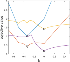
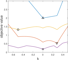
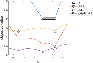
Figure 1: The objective value of different models when $a=-3$ (left), $a=3.5$ (middle), $a=4$ (right). Model parameters setting: sorted $L_{1}/L_{2}$: $t=2$, $r=5$.

In Figure 1, only our proposed sorted $L_{1}/L_{2}$ model can obtain the sparsest solution $k=0$ as the global minimizer for all the cases. The $L_{1}$ method fails when $a=-3$ while it has multiple minimizers when $a=4$. The $L_{1}/L_{2}$ regularization only gets the sparsest solution when $a=-3$, and $L_{1}$-$L_{2}$ fails for all cases.

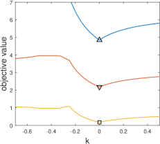
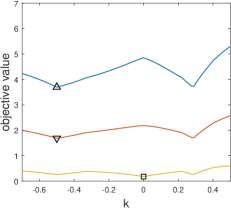
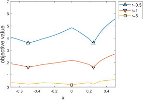
Figure 2: The effect of slope rate $r$ in the sorted $L_{1}/L_{2}$ model when $a=-3$ (left), $a=3.5$ (middle), $a=4$ (right).

Figure 2 shows that $r$ affects the scale of the objective value. A smaller value of $r$ corresponds to a larger weight thus it will result in a larger value of the numerator, as well as a smaller value of the denominator. In the case of $a=3.5$ and $a=4$, different values of $r$ lead to different optimal solutions. It is observed that when $r=5$, the sorted model can find the sparsest solution in all the cases.

3 Theoretical analysis: Solution existence

In this section, we will discuss the theoretical properties of the sorted $L_{1}/L_{2}$ model. We adapt some analysis in tao2022minimization ; zeng2021analysis to prove the solution existence of the sorted $L_{1}/L_{2}$ models in both the noise-free and noisy models. Note that $\{\mathbf{x}^{k}\}$ is called a minimizing sequence of (5), if $A\mathbf{x}^{k}=\mathbf{b}$ for all $k$ and $\lim_{k\to\infty}R_{\mathbf{w}}(\mathbf{x}^{k})=s^{\ast}$, where

$$s^{*}=\inf_{\mathbf{x}\in\mathbb{R}^{n}}\left\{R_{\mathbf{w}}(\mathbf{x})\mid A\mathbf{x}=\mathbf{b}\right\}.$$ (8)

Our analysis involves an auxiliary problem as follows

$$p^{*}:=\inf\limits_{\mathbf{x}\in\mathbb{R}^{n}}\{R_{\mathbf{w}}(\mathbf{x})\mid\mathbf{x}\in\operatorname{ker}(A)\backslash\{\mathbf{0}\}\}.$$ (9)

First, we show our proposed regularization $R_{\mathbf{w}}(\mathbf{x})$ is bounded under a mild assumption.

Lemma 1

Given a nonzero signal $\mathbf{x}\in\mathbb{R}^{n}$, if there exists $\delta>0$, such that $w_{i}\geq\delta,\forall i$ then we have

$$\delta\leq R_{\mathbf{w}}(\mathbf{x})\leq\sqrt{\|\mathbf{x}\|_{0}}\leq\sqrt{n}.$$ (10)

Proof

Here we can get a lower bound of $R_{\mathbf{w}}(\mathbf{x})$ as

$$R_{\mathbf{w}}(\mathbf{x})\geq\frac{\|\mathbf{w}\odot\mathbf{x}\|_{1}}{\|\mathbf{x}\|_{2}}\geq\frac{\|\mathbf{w}\odot\mathbf{x}\|_{2}}{\|\mathbf{x}\|_{2}}\geq\frac{\delta\|\mathbf{x}\|_{2}}{\|\mathbf{x}\|_{2}}=\delta.$$

On the other hand, we have $\|\mathbf{x}\|_{1}\leq\sqrt{\|\mathbf{x}\|_{0}}\|\mathbf{x}\|_{2}$ and $\mathbf{w}$ is sorted by the magnitude of $\mathbf{x}$ in a decreasing order, then $R_{\mathbf{w}}(\mathbf{x})\leq\frac{\|\mathbf{x}\|_{1}}{\|\mathbf{x}\|_{2}}\leq\sqrt{\|\mathbf{x}\|_{0}}\leq\sqrt{n}.$

Regarding the noise-free problem (5), it is clear to see that only when $\mathbf{b}={\bf 0}$, we have $\mathbf{x}=\bf 0$. Therefore, the global optimal solution cannot be a trivial solution $\bf 0$, if ${\bf b}\neq{\bf 0}$. Next, we show the same conclusion in the noisy case (6).

Theorem 3.1

Support $A$ is an under-determined matrix, $\mathbf{b}\in\mathrm{Im}(A)$. Denote $F(\mathbf{x}):=\lambda R_{\mathbf{w}}(\mathbf{x})+\frac{1}{2}\|A\mathbf{x}-\mathbf{b}\|_{2}^{2}.$ For sufficiently small parameter $\lambda$, the optimal solution of (6) cannot be ${\bf{0}}$.

Proof

Since $A$ is an under-determined matrix and $\mathbf{b}\in\mathrm{Im}(A)$, there exist infinitely matrix solutions in $A\mathbf{x}=\mathbf{b}$. Denote

$$\hat{\mathbf{x}}=\arg\min_{\mathbf{x}}\|\mathbf{x}\|_{2}\quad\text{ such that }\quad A\mathbf{x}=\mathbf{b}.$$

Based on Lemma 1, we have

$$F(\hat{\mathbf{x}})=\frac{\lambda\|\mathbf{w}\odot\hat{\mathbf{x}}\|_{1}}{\|\left({\bf{1}}-\mathbf{w}\right)\odot\hat{\mathbf{x}}\|_{2}}\leq\lambda\sqrt{\|\hat{\mathbf{x}}\|_{0}},$$

Hence, if $\lambda<\frac{\|\mathbf{b}\|_{2}^{2}}{2\sqrt{\|\hat{\mathbf{x}}\|_{0}}}$, then we have $F(\hat{\mathbf{x}})<\frac{\|\mathbf{b}\|_{2}^{2}}{2}=F(\mathbf{0})$, which leads the global minimizer of (6) can not be ${\bf 0}$.

Next we discuss the non-emptiness of the auxiliary problem (9) and the relationship between $s^{\ast}$ and $p^{\ast}$.

Lemma 2

Consider (9), assume $\mathbf{w}$ is larger than zero, i.e., there exists $\delta>0$, such that $w_{i}\geq\delta,\forall i$, then $p^{*}<+\infty$ and the solution of (9) is nonempty for any $A\in\operatorname{\mathbb{R}}^{m\times n}$ and $\mathbf{x}\in\operatorname{\mathbb{R}}^{n}$.

Proof

Suppose there exists an unbounded sequence $\{\mathbf{z}^{k}\}$ of (9) such that $R_{\mathbf{w}}(\mathbf{z}^{k})\to p^{*}$ as $k\to+\infty$. It implies $p^{*}<+\infty$. Defining $\hat{\mathbf{z}}^{k}=\frac{\mathbf{z}^{k}}{\|\mathbf{z}^{k}\|_{2}}$, which is bounded and belongs to $\operatorname{ker}(A)\backslash\{\mathbf{0}\}$. Owing to the scale-invariant property of the sorted $L_{1}/L_{2}$, we have $R_{\mathbf{w}}(\hat{\mathbf{z}}^{k})=R_{\mathbf{w}}(\mathbf{z}^{k})\to p^{\ast}$.Therefore, we get one accumulation point $\mathbf{z}^{\ast}\in\operatorname{ker}(A)\backslash\{\mathbf{0}\}$ from this bounded sequence. Thus we prove the solution set of $p^{*}$ is nonempty.

Lemma 3

Consider (8) and (9), for any $A\in\operatorname{\mathbb{R}}^{m\times n}$, $\mathbf{x}\in\operatorname{\mathbb{R}}^{n}$, one can obtain $s^{\ast}\leq p^{\ast}$.

Proof

For every $\mathbf{v}\in\ker(A)\setminus\{{\bf 0}\}$, we will get $s^{*}\leq R_{\mathbf{w}}(\mathbf{x}+t\mathbf{v})$, where $t\in\operatorname{\mathbb{R}}$ is a constant. Thus we derive

$$\lim_{t\to\infty}R_{\mathbf{w}}(\mathbf{x}+t\mathbf{v})=\lim_{t\rightarrow\infty}R_{\mathbf{w}}(\mathbf{x}/t+\mathbf{v})=R_{\mathbf{w}}(\mathbf{v}).$$ (11)

Eventually, we will obtain

$$s^{*}\leq R_{\mathbf{w}}(\mathbf{v}),$$ (12)

where $\mathbf{v}\in\operatorname{\mathbb{R}}^{n}$, $\mathbf{v}\in\ker(A)\setminus\{{\bf 0}\}$, which leads to $s^{\ast}\leq p^{\ast}$, directly.

By the definition in (8), we suppose there exists an unbounded minimizing sequence $\mathbf{x}^{k}$ converge to $s^{*}$, i.e., $\lim_{k\to\infty}R_{\mathbf{w}}(\mathbf{x}^{k})=s^{*}$. After that, we now prepare to prove that $p^{*}$ is equivalent to $s^{*}$.

Lemma 4

Consider (8) and (9), for any $A\in\operatorname{\mathbb{R}}^{m\times n}$, $\mathbf{x}\in\operatorname{\mathbb{R}}^{n}$, one can obtain $s^{*}=p^{*}$ if and only if there exists a minimizing sequence of (8) that is unbounded.

Proof

Suppose there is an unbounded minimizing sequence $\left\{\mathbf{x}^{k}\right\}$ of the noise-free problem (8). Without loss of generality, assume we have $\|\mathbf{x}^{k}\|_{2}\to\infty$ and denote $\lim_{k\to\infty}\frac{\mathbf{x}^{k}}{\|\left({\bf{1}}-\mathbf{w}\right)\odot\mathbf{x}^{k}\|_{2}}=\mathbf{x}^{\ast}$ for some $\mathbf{x}^{\ast}$ where $\|\mathbf{w}\odot\mathbf{x}^{\ast}\|_{1}=s^{\ast}$ according to the definition of the minimizing sequence. In addition,

$$A\mathbf{x}^{\ast}=\lim_{k\to\infty}\frac{A\mathbf{x}^{k}}{\|\left({\bf{1}}-\mathbf{w}\right)\odot\mathbf{x}^{k}\|_{2}}=\lim_{k\to\infty}\frac{\mathbf{b}}{\|\left({\bf{1}}-\mathbf{w}\right)\odot\mathbf{x}^{k}\|_{2}}={\bf 0}.$$ (13)

Hence $\mathbf{x}^{\ast}\in\ker(A)\setminus\{{\bf 0}\}$. One can obtain $\|\mathbf{(1-w)}\odot\mathbf{x}^{*}\|_{2}=1$, which implies

$$p^{*}\leq R_{\mathbf{w}}(\mathbf{x}^{\ast})=\frac{\|\mathbf{w}\odot\mathbf{x}^{\ast}\|_{1}}{\|\mathbf{(1-w)}\odot\mathbf{x}^{*}\|_{2}}=s^{*}.$$ (14)

Combining Lemma 3, we obtain $p^{*}=s^{*}$.

Now we prove the necessary condition: suppose that $s^{*}=p^{*}$, since $s^{*}<\infty$, we have a sequence $\left\{\mathbf{d}^{k}\right\}$ satisfying $\mathbf{d}^{k}\in\ker(A)\setminus\{{\mathbf{0}}\}$ such that $\lim_{k\to\infty}R_{\mathbf{w}}(\mathbf{d}^{k})=p^{*}$. Without loss of generality, assume $\lim_{k\to\infty}\frac{\mathbf{d}^{k}}{\|\mathbf{(1-w)}\odot{\mathbf{d}^{k}}\|_{2}}=\mathbf{d}^{*}$ for some $\mathbf{d}^{*}$ with $\|{\mathbf{(1-w)}}\odot{\mathbf{d}^{*}}\|_{2}=1$. It follows that

$$\begin{split}&A\mathbf{d}^{*}=\lim_{k\to\infty}\frac{A\mathbf{d}^{k}}{\|{\mathbf{(1-w)}}\odot{\mathbf{d}^{k}}\|_{2}}=\mathbf{0}\\ &\text{with}\quad\|\mathbf{w}\odot\mathbf{d}^{*}\|_{1}=\lim_{k\rightarrow\infty}R_{\mathbf{w}}(\mathbf{d}^{k})=p^{*}.\end{split}$$ (15)

Now we choose one fixed $\mathbf{\bar{x}}$ such that $A\mathbf{\bar{x}}=\mathbf{b}$ and define ${\mathbf{x}^{l}}=\mathbf{\bar{x}}+l{\mathbf{d}^{*}}$ for $l=1,2,...$. One can obtain $A{\mathbf{x}}^{l}=\mathbf{b}$ for all $l$. Thanks to (11), then the following equality achieved

$$\lim_{l\to\infty}R_{\mathbf{w}}(\mathbf{x}^{l})=\lim_{l\to\infty}R_{\mathbf{w}}(\bar{\mathbf{x}}+l\mathbf{d}^{*})=R_{\mathbf{w}}(\mathbf{d}^{*})=p^{\ast}=s^{*}$$ (16)

since $\|\mathbf{x}^{l}\|_{2}\to\infty$ as $l\to\infty$. Thus, ${\mathbf{x}^{l}}$ is an unbounded minimizing sequence for (1), which indicates our proof is complete.

In tao2023study ; zeng2021analysis ; vavasis2009derivation ; zhang2013theory , the existence of globally optimal solutions is analyzed based on the spherical section property (SSP). Here we revisit SSP and prove the solution’s existence.

Definition 1

(spherical section property vavasis2009derivation ; zhang2013theory ) Let $m$, $n$ be two positive integers such that $m<n$ and $V$ be an $(n-m)$-dimensional subspace of $\mathbb{R}^{n}$. We say that $V$ has the $s$-spherical section property if

$$\inf_{\mathbf{v}\in V\backslash\{\bf 0\}}\frac{\|\mathbf{v}\|_{1}}{\|\mathbf{v}\|_{2}}\geq\sqrt{\frac{m}{s}}.$$ (17)

Theorem 3.2

(solution existence in (5)) Consider (5), suppose that $\ker(A)$ has the sorted spherical section property for some $s>0$ and there exists $\tilde{\mathbf{x}}\in\mathbb{R}^{n}$ such that $\|\tilde{\mathbf{x}}\|_{0}<\delta^{2}m/s$ and $A\tilde{\mathbf{x}}=\mathbf{b}$. If there exists $\delta>0$, such that $w_{i}\geq\delta,\forall i$, then the set of optimal solutions of (5) is nonempty.

Proof

According to the sorted spherical property of $\ker(A)$ and the definition of $p^{*}$ in (9), one can obtain $p^{*}$ satisfies $p^{*}\geq\delta\sqrt{m/s}$. According to Lemma 1, it follows that

$$s^{*}\leq\frac{\|\mathbf{w}\odot\tilde{\mathbf{x}}\|_{1}}{\|\mathbf{(1-w)}\odot\tilde{\mathbf{x}}\|_{2}}\leq\sqrt{\|\tilde{\mathbf{x}}\|_{0}}<\delta\sqrt{\frac{m}{s}}\leq p^{*},$$ (18)

where the left term is satisfied with $A\tilde{\mathbf{x}}=\mathbf{b}$, and the middle term is due to the equivalence of norms, while the last term holds by our assumption. Thus $s^{\ast}<p^{\ast}$. Combining Lemma 4, we obtain that there is a bounded minimizing sequence $\left\{\mathbf{x}^{k}\right\}$ for (5). One can pass to a convergent subsequence $\left\{\mathbf{x}^{k_{j}}\right\}$ so that $\lim_{j\to\infty}x^{k_{j}}=\bar{\mathbf{x}}$ for some $\bar{\mathbf{x}}$ satisfying $A\bar{\mathbf{x}}=\mathbf{b}$. Since $\mathbf{b}\neq\bf 0$, it implies $\bar{\mathbf{x}}\neq\bf 0$. We then upon using the continuity of $R_{\mathbf{w}}(\mathbf{x})$ at $\bar{\mathbf{x}}$ and the definition of minimizing sequence that

$$R_{\mathbf{w}}(\bar{\mathbf{x}})=\frac{\|\mathbf{w}\odot\bar{\mathbf{x}}\|_{1}}{\|(\mathbf{1-w})\odot\bar{\mathbf{x}}\|_{2}}=\lim_{j\to\infty}\frac{\|\mathbf{w}\odot\bar{\mathbf{x}}^{k_{j}}\|_{1}}{\|(\mathbf{1-w})\odot\bar{\mathbf{x}}^{k_{j}}\|_{2}}=s^{*}.$$ (19)

This shows that $\bar{\mathbf{x}}$ is an optimal solution of (5). Then the proof is completed.

Theorem 3.3

(solution existence in (6)) Denote the infimum of the objective function as

$$F^{*}:=\inf_{\mathbf{x}\in\operatorname{\mathbb{R}}^{n}}\lambda R_{\mathbf{w}}(\mathbf{x})+\frac{1}{2}\|A\mathbf{x}-\mathbf{b}\|_{2}^{2}<\infty.$$ (20)

If $A\in\operatorname{\mathbb{R}}^{n}$ is full row rank, $\mathbf{b}\notin{\bf 0}$, there exists $\delta>0$, such that $w_{i}\geq\delta,\forall i$, and $0<\lambda<\frac{\|\mathbf{b}\|_{2}^{2}}{2(\sqrt{n}-\delta)}$, then the solution set of (6) is nonempty.

Proof

Since $A$ is full row rank, one can obtain $\tilde{\mathbf{x}}:=A^{\top}(AA^{\top})^{-1}\mathbf{b}$ such that $A\tilde{\mathbf{x}}=\mathbf{b}$. According to Theorem 3.1, there exist a sequence taking from $\{\mathbf{x}^{k}\}$ where $\mathbf{x}^{k}\neq{\bf 0}$, such that $\displaystyle\lim_{k\to\infty}F(\mathbf{x}^{k})=F^{*}$. Then we will show the optimal solution being nonempty via the following two cases:

(i) Assuming that there is only a finite number of $k$ such that $\mathbf{x}^{k}\notin\ker(A)$, without loss of generality, if erasing these elements and maintaining the rest still as $\mathbf{x}^{k}$, it will make the following inequality set up,

$$\lambda\sqrt{n}\geq F(\tilde{\mathbf{x}})\geq F^{*}=\lim_{k\rightarrow\infty}F\left(\mathbf{x}^{k}\right)\geq{\lambda}{\delta}+\frac{1}{2}\|\mathbf{b}\|_{2}^{2},$$ (21)

which violates the condition $0<\lambda<\frac{\|\mathbf{b}\|_{2}^{2}}{2(\sqrt{n}-\delta)}$.

(ii) If there are infinite number of $k$ such that $\mathbf{x}^{k}\notin\ker(A)$. Thus there must be a subsequence $\left\{\mathbf{x}^{k_{i}}\right\}$ such that $\left\{\mathbf{x}^{k}\right\}\supseteq\left\{\mathbf{x}^{k_{i}}\right\}$ with $\mathbf{x}^{k_{i}}\notin\ker(A)$. We can obtain

$$\begin{split}&\sqrt{\sigma_{\min}\left(A^{\top}A\right)}\left\|\mathbf{x}^{k_{j}}\right\|_{2}-\|\mathbf{b}\|_{2}\leq\left\|A\mathbf{x}^{k_{j}}\right\|_{2}-\|\mathbf{b}\|_{2}\\ &\leq\left\|A\mathbf{x}^{k_{j}}-\mathbf{b}\right\|_{2}\leq 2\sqrt{F^{*}}.\end{split}$$ (22)

Here the first term is the smallest eigenvalue of the matrix $A^{\top}A$. The last term is due to $\|A\mathbf{x}^{k_{i}}-\mathbf{b}\|_{2}^{2}\leq 2F(\mathbf{x}^{k_{i}})\leq 4F^{*}$ with a sufficient large subscript $i$. The result implies $\{\mathbf{x}^{k_{i}}\}$ is bounded, thus there exists a subsequence ${\mathbf{x}^{k_{i_{j}}}}$ converging to $\hat{\mathbf{x}}$ such that,

$$\lim_{j\rightarrow\infty}F(\mathbf{x}^{k_{i_{j}}})=F^{*}.$$ (23)

Thus $\hat{\mathbf{x}}\in\mathop{\arg\min}\limits_{\mathbf{x}\in\mathbb{R}^{n}}F(\mathbf{x})$, which is a global minimizer of (6), and hence the solution set is nonempty.

4 Algorithms development

This section provides algorithms for the noise-free (5) and noisy models (6).

4.1 Noise-free case

The constrained model (5) can be rewritten as

$$\min\limits_{\mathbf{x}\in\mathbb{R}^{n}}\ \ \left\{R_{\mathbf{w}}(\mathbf{x})+I_{0}(A\mathbf{x}-\mathbf{b})\right\},$$ (24)

where $I_{0}$ is an indicator function enforcing $\mathbf{x}$ to satisfy the constraint

$$I_{0}(\mathbf{t})=\begin{cases}0&\mbox{if }\mathbf{t}={\bf 0},\\ +\infty&\text{otherwise}.\end{cases}$$ (25)

Here we adopt a DCA-type algorithm to solve the problem (24). Note that DCA is a descent algorithm for minimizing the difference of convex (DC) functions TA98 ; phamLe2005dc . Here, we use the same scheme but relax the limitation of convex functions. Generally, DCA splits the objective function into two terms $G$ and $H$:

$$\min_{\mathbf{x}\in\mathbb{R}^{m}}F(\mathbf{x}):=G(\mathbf{x})-H(\mathbf{x}).$$

Starting from an initial point $\mathbf{x}^{0}$, DCA iteratively constructs two sequences $\left\{\mathbf{x}^{k}\right\}$ and $\left\{\mathbf{y}^{k}\right\}$:

$$\left\{\begin{array}[]{l}\mathbf{y}^{k}\in\partial H\left(\mathbf{x}^{k}\right)\\ \mathbf{x}^{k+1}\in\operatorname*{arg\,min}\limits_{\mathbf{x}}G(\mathbf{x})-\left\langle\mathbf{x},\mathbf{y}^{k}\right\rangle,\end{array}\right.$$

where $\mathbf{y}^{k}\in\partial H\left(\mathbf{x}^{k}\right)$, i.e., $\mathbf{y}^{k}$ is a subgradient of $H(\mathbf{x})\text{ at }\mathbf{x}^{k}.$ In our problem (24), we consider the decomposition as follows:

$$\begin{split}G(\mathbf{x})&=\alpha\|\mathbf{x}\|_{1}+I_{0}(A\mathbf{x}-\mathbf{b}),\\ H(\mathbf{x})&=\alpha\|\mathbf{x}\|_{1}-R_{\mathbf{w}}(\mathbf{x}).\end{split}$$ (26)

Here $G(x)$ is convex, but $H(x)$ may may not be. Note that the selection of the weight guarantee $\|\mathbf{(1-w)}\odot\mathbf{x}\|_{2}$ does not equal zero, and we get

$$\begin{split}\partial H(\mathbf{x})&=\alpha\partial\|\mathbf{x}\|_{1}-\frac{\partial\|\mathbf{w}\odot\mathbf{x}\|_{1}}{\|\left({\bf{1}}-\mathbf{w}\right)\odot\mathbf{x}\|_{2}}+\frac{\|\mathbf{w}\odot\mathbf{x}\|_{1}(1-\mathbf{w})^{2}\odot\mathbf{x}}{\|\left({\bf{1}}-\mathbf{w}\right)\odot\mathbf{x}\|_{2}^{3}}.\end{split}$$ (27)

Therefore, $\mathbf{y}^{k}$ can be set as $\mathbf{y}^{k}=\alpha\operatorname{sign}(\mathbf{x}^{k})-\frac{\operatorname{sign}(\mathbf{w}\odot\mathbf{x}^{k})}{\|\left({\bf{1}}-\mathbf{w}\right)\odot\mathbf{x}^{k}\|_{2}}+\frac{\|\mathbf{w}\odot\mathbf{x}^{k}\|_{1}(1-\mathbf{w})^{2}\odot\mathbf{x}^{k}}{\|\left({\bf{1}}-\mathbf{w}\right)\odot\mathbf{x}^{k}\|_{2}^{3}},$ where $\operatorname{sign}(\mathbf{v})$ is a signum function $\operatorname{sign}(\mathbf{v})_{i}=\begin{cases}1&v_{i}>0,\\ 0&v_{i}=0,\\ -1&v_{i}<0.\end{cases}$ After computing $\mathbf{y}^{k}$, the $\mathbf{x}$-subproblem can be formulated as a linear programming problem. Notice that

$$\mathbf{x}^{k+1}=\operatorname*{arg\,min}_{\mathbf{x}}\left\{\alpha\|\mathbf{x}\|_{1}+I_{0}(A\mathbf{x}-\mathbf{b})-\left\langle\mathbf{x},\mathbf{y}^{k}\right\rangle\right\},$$ (28)

which can be formulated into a linear programming (LP) problem by nonnegative transformation with $\mathbf{x}$. Assume $\mathbf{x}\in\operatorname{\mathbb{R}}^{n}$ can be split into the minus of two nonnegative parts $\mathbf{x}=\mathbf{x}^{+}-\mathbf{x}^{-}$, where $\mathbf{x}^{+}\geq{\bf 0}$ and $\mathbf{x}^{-}\geq{\bf 0}$ and let $\hat{\mathbf{x}}=\begin{bmatrix}\mathbf{x}^{+}\\ \mathbf{x}^{-}\end{bmatrix}$. Then the linear constraint $A\mathbf{x}=\mathbf{b}$ turns to $\bar{A}\hat{\mathbf{x}}=\mathbf{b}$ where $\bar{A}=\left[A-A\right]$. Then the problem will be

$$\min_{\mathbf{x}\geq 0}\mathbf{1}^{T}\mathbf{x}\quad\text{ s.t. }\quad\bar{A}\mathbf{x}=\mathbf{b},$$

thus after deriving the solution $\hat{\mathbf{x}}$, we could obtain the solution $\mathbf{x}$ by

$$\mathbf{x}=\hat{\mathbf{x}}(1:n)-\hat{\mathbf{x}}(n+1:2n).$$

Besides, since we have the indicator function in $G(\mathbf{x})$, we could formulate it to

$$\mathbf{x}^{k+1} =\operatorname*{arg\,min}_{\mathbf{x}}\left\{\alpha\|\mathbf{x}\|_{1}+I_{0}(A\mathbf{x}-\mathbf{b})-\left\langle x,\partial H\left(\mathbf{x}^{k}\right)\right\rangle\right\}$$ (29)

$$=\operatorname*{arg\,min}_{\mathbf{x}}\left\{\alpha\|\mathbf{x}\|_{1}-\left\langle\mathbf{x},\mathbf{y}^{k}\right\rangle\quad\text{s.t. }A\mathbf{x}=\mathbf{b}\right\},$$

which can be efficiently solved by an optimization software called Gurobi.

In addition, since we do not assume to know the order of the magnitude in the ground truth signal $\bar{\mathbf{x}}$. We sort the entries of $\mathbf{x}^{k}$ during each iteration and update the weight accordingly. The algorithm is summarized as Algorithm 1.

Algorithm 1 The sorted $L_{1}/L_{2}$ minimization via DCA-type algorithm in the noise-free case.

  Input: $A\in\mathbb{R}^{m\times n},\mathbf{b}\in\mathbb{R}^{m\times 1}$, Max and $\epsilon\in\mathbb{R}$, $\rho\in R$

  Initialization: $k=1$ and solve the $L_{1}$ minimization to get $\mathbf{x}^{1}$

  while $k<$ Max or $\|\mathbf{x}^{k}-\mathbf{x}^{k-1}\|_{2}/\|\mathbf{x}^{k}\|>\epsilon$ do

     $\mathbf{y}^{k}=\alpha\operatorname{sign}(\mathbf{x}^{k})-\frac{\operatorname{sign}(\mathbf{w}\odot\mathbf{x}^{k})}{\|\mathbf{x}^{k}-\mathbf{w}\odot\mathbf{x}^{k}\|_{2}}+\frac{\|\mathbf{w}\odot\mathbf{x}^{k}\|_{1}(1-\mathbf{w})^{2}\odot\mathbf{x}^{k}}{\|\mathbf{x}^{k}-\mathbf{w}\odot\mathbf{x}^{k}\|_{2}^{3}}$

     Adopt Gurobi to solve the linear programming problem and obtain $\mathbf{x}^{k}$

     Update the weight $\mathbf{w}$ based on $\mathbf{x}^{k}$

     $k=k+1$

  end while

  return  $\mathbf{x}^{k}$

4.2 Noisy case

We consider the unconstrained model (6). Similar to the noise-free case, we first use a DCA-type scheme to split the optimization problem to be two-part:

$$\begin{split}&G(\mathbf{x})=\alpha\|\mathbf{x}\|_{1}+\frac{1}{2}\|A\mathbf{x}-\mathbf{b}\|_{2}^{2}\\ &H(\mathbf{x})=\alpha\|\mathbf{x}\|_{1}-\lambda R_{\mathbf{w}}(\mathbf{x}),\end{split}$$ (30)

where $\alpha$ is the parameter about the degree of convexity in each term. Here $\partial H(\mathbf{x})$ is exactly the same as (27) in the noise-free case except we have a regularization parameter for the sorted penalty. Note that through the DCA-type splitting, we only need to solve the unconstrained quadratic programming problem,

$$\mathbf{x}^{k+1}=\operatorname*{arg\,min}_{\mathbf{x}\in\mathbb{R}^{n}}\ \alpha\|\mathbf{x}\|_{1}+\frac{1}{2}\|A\mathbf{x}-\mathbf{b}\|_{2}^{2}-\left<\mathbf{x},\mathbf{y}^{k}\right>,$$ (31)

where $\mathbf{y}^{k}=\partial H(\mathbf{x}^{k})$. Here we utilize the alternating direction method of multipliers (ADMM) to solve the subproblem. By introducing $\mathbf{z}\in\operatorname{\mathbb{R}}^{n}$ as the auxiliary variable, the optimization problem can be rewritten as:

$$\operatorname*{arg\,min}_{\mathbf{x},\mathbf{z}\in\mathbb{R}^{n}}\alpha\|\mathbf{z}\|_{1}+\frac{1}{2}\|A\mathbf{x}-\mathbf{b}\|_{2}^{2}-\left<\mathbf{z},\mathbf{y}^{k}\right>\quad\mathrm{s.t.}\ \ \mathbf{x}=\mathbf{z}.$$ (32)

The augmented Lagrangian can be illustrated as:

$$L_{\delta}^{k}(\mathbf{x},\mathbf{z};\mathbf{v})=\alpha\|\mathbf{z}\|_{1}+\frac{1}{2}\|A\mathbf{x}-\mathbf{b}\|_{2}^{2}-\left<\mathbf{z},\mathbf{y}^{k}\right>+\frac{\delta}{2}\left\|\mathbf{x}-\mathbf{z}+\mathbf{v}\right\|_{2}^{2}.$$ (33)

Here the problem just generates two subproblems with a scaled dual variable updating the residual at the next iteration:

$$\left\{\begin{array}[]{l}\mathbf{x}_{j+1}:=\operatorname*{arg\,min}\limits_{\mathbf{x}}L_{\delta}^{k}(\mathbf{x},\mathbf{z}_{j};\mathbf{v}_{j}),\\ \mathbf{z}_{j+1}:=\operatorname*{arg\,min}\limits_{\mathbf{z}}L_{\delta}^{k}(\mathbf{x}_{j+1},\mathbf{z};\mathbf{v}_{j}),\\ \mathbf{v}_{j+1}:=\mathbf{v}_{j}+\mathbf{z}_{j+1}-\mathbf{x}_{j+1},\\ \end{array}\right.$$ (34)

where the subscript $j$ represents the inner loop index, as opposed to the superscript $k$ for outer iterations. For the subproblem of $\mathbf{x}$, since (33) is a quadratic function, the minimization of subproblem $\mathbf{x}$ can be reformulated as the proximal, then the closed-form solution will be

$$\mathbf{x}_{j+1}=(A^{\top}A+\delta I)^{-1}(A^{\top}\mathbf{b}+\delta(\mathbf{z}_{j}+\mathbf{v}_{j})).$$ (35)

Then the subproblem of solving $\mathbf{z}$ is the solution of the soft-threshold operator,

$$\mathbf{z}_{j+1}=\operatorname{shrink}\left(\mathbf{x}_{j+1}-\mathbf{v}_{j}+\mathbf{y}^{k},\frac{\alpha}{\delta}\right),$$ (36)

where

$$\operatorname{shrink}(\mathbf{x},a)_{i}=\begin{cases}x_{i}+a&x_{i}<-a,\\ 0&-a\leq x_{i}\leq a,\\ x_{i}-a&x_{i}>a.\end{cases}$$

The last multiplier can be updated with the residual of $\mathbf{z}$ and $\mathbf{x}$ at iteration $j+1$.

$$\mathbf{v}_{j+1}=\mathbf{v}_{j}+\mathbf{z}_{j+1}-\mathbf{x}_{j+1}.$$ (37)

The algorithm is summarized as Algorithm 2.

Algorithm 2 The sorted $L_{1}/L_{2}$ minimization via DCA-type scheme in the case of the noisy case.

  Input: $A\in\mathbb{R}^{m\times n},\mathbf{b}\in\mathbb{R}^{m\times 1}$, kMax, jMax, $\epsilon\in\mathbb{R}$, and $\rho\in R$

  Initialization: $k=1$, and solve for the $L_{1}$ minimization to get $\mathbf{x}^{0}$

  while $k<$ kMax or $\|\mathbf{x}^{k}-\mathbf{x}^{k-1}\|_{2}/\|\mathbf{x}^{k}\|>\epsilon$ do

     $\mathbf{y}^{k}=\alpha\operatorname{sign}(\mathbf{x}^{k})-\frac{\lambda\operatorname{sign}(\mathbf{w}\odot\mathbf{x}^{k})}{\|\mathbf{x}^{k}-\mathbf{w}\odot\mathbf{x}^{k}\|_{2}}+\frac{\lambda\|\mathbf{w}\odot\mathbf{x}^{k}\|_{1}(1-\mathbf{w})^{2}\odot\mathbf{x}^{k}}{\|\mathbf{x}^{k}-\mathbf{w}\odot\mathbf{x}^{k}\|_{2}^{3}}$

     while $j<$jMax or $\|\mathbf{x}_{j}-\mathbf{x}_{j-1}\|_{2}/\|\mathbf{x}_{j}\|>\epsilon$ do

        $\mathbf{x}_{j+1}=(A^{\top}A+\delta I)^{-1}(A^{\top}\mathbf{b}+\delta(\mathbf{z}_{j}+\mathbf{v}_{j})$

        $\mathbf{z}_{j+1}=\operatorname{shrink}\left(\mathbf{x}_{j+1}-\mathbf{v}_{j}+\mathbf{y}^{k},\frac{\alpha}{\delta}\right)$

        $\mathbf{v}_{j+1}=\mathbf{v}_{j}+\mathbf{z}_{j+1}-\mathbf{x}_{j+1}$

        $j=j+1$

     end while

     $\mathbf{x}^{k+1}=\mathbf{x}_{j}$

     Update the weight $\mathbf{w}$ based on $\mathbf{x}^{k+1}$

     $k=k+1$

  end while

  return  $\mathbf{x}^{k}$

5 Numerical results

In this section, we will demonstrate the performance of the proposed methods via a series of numerical experiments. All the numerical experiments are conducted on a standard laptop with CPU(AMD Ryzen 5 4600U at 2.10GHz) and MATLAB (R2021b).

In the noise-free case, we test two types of special sensing matrices, oversampled discrete cosine transform (DCT), and Gaussian random matrix. For over-sample DCT experiments, we follow the works DCT2012coherence ; louYHX14 ; yinLHX14 to define $A=[\mathbf{a}_{1},\mathbf{a}_{2},\dots,\mathbf{a}_{n}]\in\mathbb{R}^{m\times n}$ with

$$\mathbf{a}_{j}:=\frac{1}{\sqrt{m}}\cos\left(\frac{2\pi\mathbf{h}j}{F}\right),\quad j=1,\dots,n,$$ (38)

where $\mathbf{h}$ is a random vector independently sampled and uniformly distributed in $[0,1]^{m}$. Here $F\in Z^{+}$ controls the coherence, i.e., with $F$ increasing, the column of the sensing matrix becomes more coherent. Matrix with high coherence results in an ill-posedness, in which one can see that the coherence is generally describing the multicollinearity of matrix $A$. On the other hand, we generate a Gaussian random matrix by using $\mathcal{N}(\mathbf{0},\Sigma)$, where $\Sigma=\{(1-R)*I(i=j)+R\}_{i,j}$ with a positive parameter $R$. Note that a larger value of $R$ will lead to greater difficulty in recovering the sparsest solution zhangX18 . Besides, we generate the support index of the ground truth $\mathbf{\bar{x}}\in\operatorname{\mathbb{R}}^{n}$ by the unified distribution with entries following the standard normal distribution. Then we normalize the whole ground truth to enforce its maximum to be 1. The measurements $\mathbf{b}$ can be generated naturally by the product of sensing matrix $A$ and the ground truth $\mathbf{x}$. All tests on sparse recovery obey the same environment setting. We set the size of sensing matrices $64\times 1024$ to test the performance with a severely ill-posed problem. In addition, in the previous work doi:10.1137/110838509 , they have shown there is a minimum separation between these adjacent support index of $\bar{\mathbf{x}}$, recovering the sparsest solution could be possible. Here throughout the noise-free case, we impose all the models satisfying that: $\min_{i,i^{\prime}\in\operatorname{supp}(\overline{\mathbf{x}})}\left|i-i^{\prime}\right|\geq 1$ for both the oversampled-DCT and Gaussian sensing matrices. For the measure of performance, we take the relative error (ReErr) between the reconstruction solution $\mathbf{x}$ and the ground truth $\bar{\mathbf{x}}$, defined as $\|\mathbf{x}-\overline{\mathbf{x}}\|_{2}/\|\overline{\mathbf{x}}\|_{2}$. Furthermore, Now we define the success rate: the number of successful trials over the total number of trials. If ReErr $<10^{-3}$, then we treat it as a successful trial to recover the ground truth. We adopt a commercial optimization software Gurobi optimization2014inc to minimize the $L_{1}$ norm via linear programming for the sake of efficiency. We restrict the values of $\mathbf{x}^{+}$ and $\mathbf{x}^{-}$ within $[0,1]$, owing to the normalization. The stopping criterion is when the relative error of $\mathbf{x}^{k}$ to $\mathbf{x}^{k-1}$ is smaller than $10^{-8}$ or iterative number exceeds $10n$.

The experiments in the noisy case follow a setup in 6205396 . We focus on recovering a signal $\mathbf{x}$ of length $n=512$ with $s=130$ nonzero elements from $m$ measurements, represented by $\mathbf{b}$, obtained through a Gaussian random matrix $A$. The matrix $A$ has normalized columns with a zero mean and a unit Euclidean norm, and Gaussian noise with zero mean and standard deviation $\sigma=0.1$ is also taken into account. Fewer $m$ leads to a more difficult and ill-posed problem for the reconstruction. We use the mean-square error (MSE) metric to assess the recovery performance. Since the sorted $L_{1}/L_{2}$ model is a nonconvex-type model, the choice of initial guess $\mathbf{x}^{(0)}$ directly impacts the performance. We use the restored solution via the $L_{1}$ minimization as the initial guess throughout the noise-free and noisy case.

5.1 Discussion on weight vector

We consistently utilize the same weight vector as (7) throughout all the numerical experiments. Here $t$ controls the cardinality of $\Gamma_{\mathbf{x},t}$, and $r$ is the “slope rate” to determine the shape of $\mathbf{w}$, where a large $r$ clearly leads to a large curvature. Due to the uncertainty of the performance of support detection by $L_{1}$ initial guess, we choose $t$ around ${\|\mathbf{x}_{L_{1}}\|_{0}}/{3}$ which is similar to one in huang2015nonconvex . Here $\mathbf{x}_{L_{1}}$ is the restored signal via $L_{1}$. Furthermore, it is noteworthy that since the weight is an exponential function, a large $r$ will cause a significant proportion of $\left\{w_{i}\right\},i\in\Gamma_{\mathbf{x},t}$ values clustering at very small values. Hence, selecting a small value for $r$ is a suitable choice at the beginning. In addition, in Figure 2, one can observe that a small value of $r$ can amplify the scale of local optimums and makes them sharper, which can improve the probability of the model encountering the local optimum.

Furthermore, we devise a two-stage weighting scheme. In the first stage, we use small values of $t$ and $d$ to encourage finding more entries in the support. After the 20 iteration step, we alter the value of the weight function to accelerate the support detection and the convergence. To be precise, in the absence of noise, we employ $(t,r)=(20,0.8)$ in the first stage and $(t,r)=(27,3)$ in the second stage, whereas, for the noisy case, we choose $(t,r)=(100,0.8)$ and $(t,r)=(120,3)$ in the respective stages. Figure 3 shows the noise-free case, where the left sub-figure is the shape of the weight vector sorted in ascending order. Note that changing the value of $t$ not only modifies values of the weight function but also implies a desire to encompass more possible support sets that might have been overlooked. Figure 3 shows that the two-stage scheme has higher success rates for sparse recovery than the one-stage, especially when the sparsity level is high.

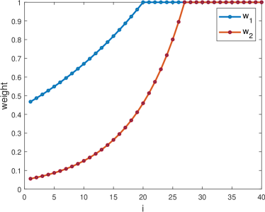
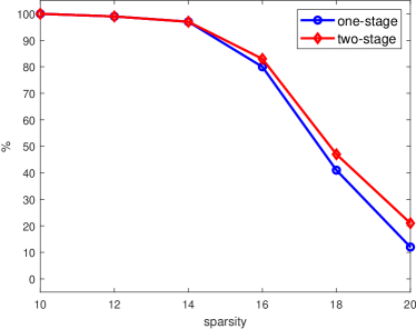
Figure 3: Left: two weight functions sorted in an ascending order, where $\mathbf{w}_{1}$ and $\mathbf{w}_{2}$ are with the parameters $(t,r)=(27,3)$, and $(27,0.8)$, respectively. Right: comparison of success rate with one-stage and two-stage sorted $L_{1}/L_{2}$ in the noise-free case under the Gaussian random matrix with $R=0.1$.

5.2 Algorithm behaviors

We conduct a numerical experiment to empirically demonstrate the convergence of the proposed algorithms. In the noise-free case, the relative error and objective value decrease steeply in the first 10 iterations, as shown Figure 4. The relative error reaches to the computation accuracy $10^{-15}$ in the 9-th iteration.

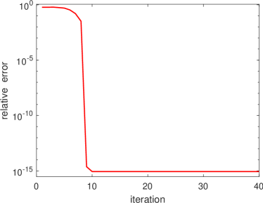
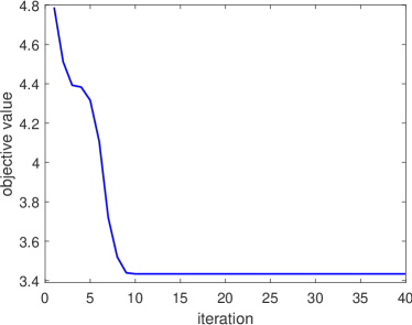
Figure 4: The relative error (left) and objective value (right) for empirically demonstrating the fast convergence of the proposed algorithm for the noise-free model.

Regarding the noisy case, Figure 5 shows the change of the objective value and relative error with different maximum iterations in the inner loop. Here maximum iteration for the outer one is set as 100. Note that with the inner iteration increasing, curves of objective value and relative error both have larger curvatures, which empirically show a more rapid convergence rate. Meanwhile, only one inner iteration will cause the objective value to rise steeply and then decrease. Besides, although a large number of inner iterations will result in a more rapid convergence, it takes much more computational time. We observe that 20 iterations in the inner loop are sufficient to yield good results. Hence, in the following experiments, we fix the maximum number of the inner iteration as 20.

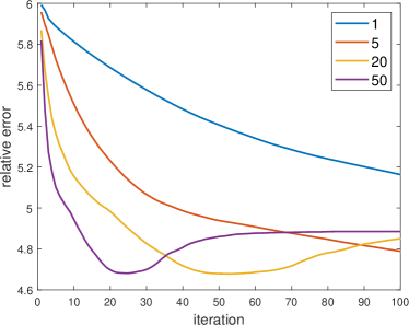
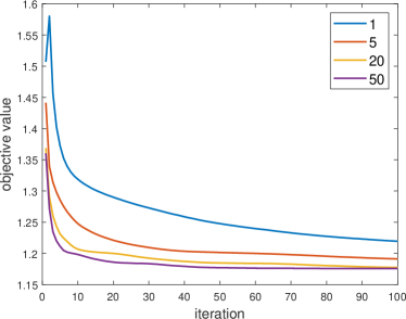
Figure 5: The relative error and objective value with different inner iterations $1,5,20,100$ for empirically demonstrating the convergence with the noisy model.

5.3 Comparison on various models

First, we consider the noise-free case and compare the proposed sorted $L_{1}/L_{2}$ minimization with four models for sparse recovery: the $L_{1}$ minimization, the $L_{p}$ modelchartrand07 , the $L_{1}$-$L_{2}$ model zibulevsky2010l1 ; lou2018fast and the $L_{1}/L_{2}$ minimization rahimi2019scale . Figure 6 reveals that the sorted $L_{1}/L_{2}$ model makes the state-of-art performance with the oversampled-DCT matrix, especially when $F=5$ with relatively low coherence. For a relatively low coherence, the $L_{1}$-$L_{2}$ minimization makes the third best, but it makes the best when $F=10$, while the sorted $L_{1}/L_{2}$ makes the second best. The $L_{1}/L_{2}$ model makes the second best and achieves a similar performance compared to the sorted $L_{1}/L_{2}$ model when $F=10$. The $L_{p}$ method does not perform well in the high coherence $F=10$, which is even worse than $L_{1}$. Regarding the Gaussian sensing matrix case, Figure 7 shows that $L_{p}$ is very excellent. We can clearly see the sorted $L_{1}/L_{2}$ model gets comparable results compared to the $L_{p}$ model both for $R=0.1$ and $R=0.8$. While $L_{1}$-$L_{2}$ performs well using oversampled-DCT in high-coherence situations, its performance worsens in the Gaussian matrix case. It is noteworthy that we use the same settings and parameters across different matrices or coherence levels and the robustness of the sorted $L_{1}/L_{2}$ model.

$F=5$	$F=10$

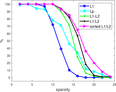
Figure 6: Success rates for different models under the oversampled-DCT matrix.

$R=0.1$	$R=0.8$

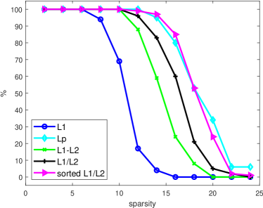
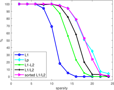
Figure 7: Success rates for different models under the Gaussian matrix.

Now we consider the noisy case and compare the proposed sorted $L_{1}/L_{2}$ model with other models in the noisy case: $L_{1}$, $L_{1}$-$L_{2}$ zibulevsky2010l1 , $L_{p}$ via the half-thresholding method 6205396 , error function for sparse recovery (ERF) guo2021novel and the oracle performance in recovering a noisy signal. In addition, we implement and compare the $L_{1}/L_{2}$ minimization in the unconstrained formulation via a DCA-type scheme. If the ground truth of support set of $\mathbf{s}=\operatorname{supp}(\mathbf{x})$ is known, which is the index set of nonzero entries in $\bar{\mathbf{x}}$, then we can give the ordinary least square (OLS) solution. Thus we take the MSE of OLS as an oracle performance with $\sigma\mathrm{tr}(A_{s}^{\top}A_{s})^{-1}$, as the benchmark.

Regarding parameter settings for the noisy sparse recovery, we set $\delta=0.8$ and $\alpha=0.1$ in our model. As for $\lambda$, we observe that a smaller value leads to better performance for smaller $m$ (which corresponds to more challenging problems), while a larger value of $\lambda$ is required for larger $m$ (which corresponds to easier problems) to increase the constraint on the penalty term and prevent over-fitting. Since earlier research has indicated that selecting a fixed penalty parameter that is either too small or too large may lead to a substantial increase in computational expenses. Here we implement the regularization parameter $\lambda$ for an adaptive updating strategy resembling the related topic hu2012fast . Note that a similar parameter setting ($\lambda=0.1\times m/270$) is used for $L_{1}$, while we empirically use $m^{2}/n^{2}-0.1$ for our model as the number of rows $m$ and columns $n$ is given. It should be noted that this parameter setting is empirical, and the performance is not sensitive to small oscillations with $\lambda$. For other models, we follow the setting from the previous work except for $L_{1}/L_{2}$, in which we adopt the DCA with parameters $\lambda=0.06,\alpha=0.05$, and $\delta=0.9$. The initial guess for all models is the solution obtained from $L_{1}$.

In Figure 8 and Table 1, the measurements are taken at 10 intervals ranging from 250 to 360. The oracle performance is based on the OLS given the support of the ground truth, which is extremely difficult to achieve. However, our proposed model closely approximates the oracle performance, especially with a large number of rows $m$, and achieves state-of-the-art performance with any $m$. As $m$ decreases, the problem becomes more ill-posed, and the performance of all models starts to converge the same.

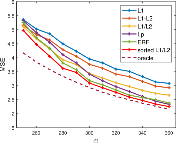
Figure 8: MSE of sparse recovery in the noisy case by different models.

Table 1: MSE of sparse recovery in the noisy case.

$m$	250	260	270	280	290	300
$L_{1}$	5.36	5.02	4.85	4.49	4.23	3.95
$L_{1}$-$L_{2}$	5.16	4.82	4.63	4.28	4.05	3.76
$L_{1}/L_{2}$	5.11	4.67	4.31	3.92	3.75	3.43
$L_{p}$	5.32	4.89	4.55	4.10	3.81	3.41
ERF	5.26	4.70	4.34	3.81	3.57	3.17
sorted $L_{1}/L_{2}$	4.98	4.50	4.06	3.63	3.47	3.10
oracle	4.17	3.84	3.57	3.33	3.12	2.93
$m$	310	320	330	340	350	360
$L_{1}$	3.81	3.59	3.51	3.32	3.13	3.08
$L_{1}$-$L_{2}$	3.62	3.41	3.32	3.15	2.98	2.92
$L_{1}/L_{2}$	3.27	3.10	2.97	2.83	2.72	2.66
$L_{p}$	3.17	2.96	2.79	2.61	2.44	2.33
ERF	3.03	2.84	2.66	2.57	2.50	2.38
sorted $L_{1}/L_{2}$	2.90	2.73	2.58	2.46	2.32	2.24
oracle	2.76	2.62	2.49	2.37	2.26	2.16

5.4 Support detection

In this section, we will conduct a series of numerical experiments to state the ability to detect support in different models. The performance of detecting support is assessed in terms of the recall rate, defined as the ratio of the number of identified true nonzero entries over the total number of true nonzero entries, and the precision rate, defined as the ratio of the number of identified true nonzero entries over the number of all the nonzero entries obtained by the algorithm. We compare the proposed model with the $L_{1}$, $L_{1}$-$L_{2}$, and $L_{1}/L_{1}$ minimization for sparsity 10, 12, 14, 16, 18, 20. Note that we consider the Gaussian sensing matrix $A$ with the same parameter setting as in Session 5.3. Each sparsity corresponds to 100 independent repeated trials, and then we take their average to calculate the recall and precision rates.

Figure 9 exhibits the proposed sorted $L_{1}/L_{2}$ minimization achieves the state-of-art recall and precision rate compared with other models. The recall rate of the sorted $L_{1}/L_{2}$ model is higher than $L_{1}$ and $L_{1}/L_{2}$ minimization, which indicates its good performance in detecting the true support. The $L_{1}$ model achieves almost 50% support index in the sparsity 20. Such performance is significantly higher than its result in sparse recovery, which implies $L_{1}$ can indeed detect the support but fail to recover the exact solution. $L_{1}/L_{2}$ performs the second best. The results in Figure 9 (right) demonstrate that the sorted $L_{1}/L_{2}$ model achieves an exceptional level of precision in various sparsity. At sparsity levels ranging from 10 to 14, our model exhibited a perfect precision of nearly average 100%, which indicates that all the non-zero elements are detected by the model. In comparison, $L_{1}$ achieves a precision of less than 30% at a sparsity level of 12 and remains steady at around 15%. The performance of $L_{1}/L_{2}$ is inferior to that of our model, as it maintained good precision at low sparsity levels. However, as the sparsity level increased, such as at the level of 18 and 20, our model demonstrates a superiority of 28% and 17% over $L_{1}/L_{2}$, respectively.

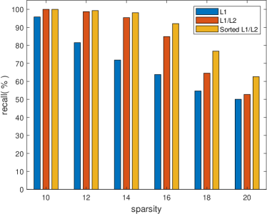
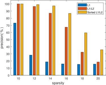
Figure 9: The recall (left) and precision rates (right) for the $L_{1}$, $L_{1}/L_{2}$, and sorted $L_{1}/L_{2}$ models with sparsity from 10 to 20.

Table 2: The rate of finding support focused on the indices with the $\|\bar{\mathbf{x}}\|_{0}$-largest magnitudes by different models with 100 independent trials. All models achieved the best when sparsity 1-9 except for $L_{1}$ thus we omit in the table.

$Sparsity$	10	12	14	16	18	20
$L_{1}$	83%	55%	35%	21%	14%	11%
$L_{1}$-$L_{2}$	100%	96%	81%	52%	25%	17%
$L_{1}/L_{2}$	100%	100%	90%	72%	41%	24%
sorted $L_{1}/L_{2}$	100%	98%	96%	87%	64%	44%

At last, we design an intriguing but straightforward experiment of variable selection. Figure 9 shows that there are a lot of nonzero entries selected by $L_{1},L_{1}/L_{2}$, or the sorted $L_{1}/L_{2}$ model. Thus we can select from the indices with large magnitudes to guarantee a high probability of detecting some true support. In light of this statement, we only consider the entries with $\|\bar{\mathbf{x}}\|_{0}$-largest magnitudes in the restored signal $\mathbf{x}$. To be more precise, for example, given sparsity 20, we only focus on the 20 largest magnitudes indexes, and then we compute the rate of finding the true support index.

Table 2 shows our proposed sorted $L_{1}/L_{2}$ model achieved state-of-art performance compared with other models. For sparsity 18, our proposed model can find the average of 64%, i.e. nearly 11 true support in 18 nonzero entries indices, while $L_{1}$, $L_{1}$-$L_{2}$, and $L_{1}/L_{2}$ only find 2, 4, and 7, respectively. As the sparsity level rises, our proposed model stays to find the average of 8 true support, which is two times that of the $L_{1}/L_{2}$ model.

6 Conclusion and future works

In this paper, we discuss a novel type of regularization by generalizing the $L_{1}/L_{2}$ model into a sorted $L_{1}/L_{2}$ scheme. We provide a theoretical analysis of the existence of solutions. By employing the DCA-type scheme, we can achieve state-of-the-art performance for sparse recovery in both noise-free and noisy scenarios. The experimental results demonstrate that the sorted model has a significant advantage over the $L_{1}/L_{2}$ model and is capable of detecting the support set with high accuracy, even in high-sparsity cases. These sorted models can be easily incorporated with a box constraint if it is available, which ensures the boundedness of the solution in the subproblem. Note that it is possible that the solution of our algorithm can be unbounded if there is no box constraint. However, we empirically test that $\{\mathbf{x}^{k}\}$ from the noise-free or noisy scenarios is always bounded and convergent for general random matrices $A$. Our future research will involve extending this sorted model to the matrix and tensor formulation to consider low-rankness instead of sparsity. Furthermore, we plan to explore its application to image processing and investigate sparsity on the gradient.

Data Availability

The MATLAB codes and datasets generated and/or analyzed during the current study will be available after publication.

Declarations

The authors have no relevant financial or non-financial interests to disclose. The authors declare that they have no conflict of interest.

References

- (1) Andreani, R., Birgin, E.G., Mart, J.M., Schuverdt, M.L.: On augmented lagrangian methods with general lower-level constraints. SIAM Journal on Optimization 18(4), 1286–1309 (2008)
- (2) Candes, E.J., Tao, T.: Decoding by linear programming. IEEE transactions on information theory 51(12), 4203–4215 (2005)
- (3) Chartrand, R.: Exact reconstruction of sparse signals via nonconvex minimization. IEEE Signal Processing Letters 10(14), 707–710 (2007)
- (4) Donoho, D.L.: Compressed sensing. IEEE Transactions on information theory 52(4), 1289–1306 (2006)
- (5) Fan, J., Li, R.: Variable selection via nonconcave penalized likelihood and its oracle properties. Journal of the American Statistical Association 96(456), 1348–1360 (2001)
- (6) Fannjiang, A., Liao, W.: Coherence pattern–guided compressive sensing with unresolved grids. SIAM Journal on Imaging Sciences 5(1), 179–202 (2012)
- (7) Fannjiang, A., Liao, W.: Coherence pattern–guided compressive sensing with unresolved grids. SIAM Journal on Imaging Sciences 5(1), 179–202 (2012). DOI 10.1137/110838509. URL https://doi.org/10.1137/110838509
- (8) Ge, H., Chen, W., Ng, M.K.: Analysis of the ratio of and norms for signal recovery with partial support information. Information and Inference: A Journal of the IMA 12(3), iaad015 (2023). DOI 10.1093/imaiai/iaad015. URL https://doi.org/10.1093/imaiai/iaad015
- (9) Guo, W., Lou, Y., Qin, J., Yan, M.: A novel regularization based on the error function for sparse recovery. Journal of Scientific Computing 87(1), 31 (2021)
- (10) Hu, Y., Zhang, D., Ye, J., Li, X., He, X.: Fast and accurate matrix completion via truncated nuclear norm regularization. IEEE transactions on pattern analysis and machine intelligence 35(9), 2117–2130 (2012)
- (11) Huang, X.L., Shi, L., Yan, M.: Nonconvex sorted l1 minimization for sparse approximation. Journal of the Operations Research Society of China 3(2), 207–229 (2015)
- (12) Lou, Y., Yan, M.: Fast - minimization via a proximal operator. Journal of Scientific Computing 74(2), 767–785 (2018)
- (13) Lou, Y., Yin, P., He, Q., Xin, J.: Computing sparse representation in a highly coherent dictionary based on difference of and . Journal of Scientific Computing 64(1), 178–196 (2015)
- (14) Lou, Y., Yin, P., Xin, J.: Point source super-resolution via non-convex l1 based methods. Journal of Scientific Computing 68, 1082–1100 (2016)
- (15) Lv, J., Fan, Y.: A unified approach to model selection and sparse recovery using regularized least squares. The Annals of Statistics pp. 3498–3528 (2009)
- (16) Ma, T.H., Lou, Y., Huang, T.Z.: Truncated l_1-2 models for sparse recovery and rank minimization. SIAM Journal on Imaging Sciences 10(3), 1346–1380 (2017)
- (17) Natarajan, B.K.: Sparse approximate solutions to linear systems. SIAM journal on computing pp. 227–234 (1995)
- (18) Optimization, G.: Gurobi optimizer reference manual (2015)
- (19) Peleg, T., Gribonval, R., Davies, M.E.: Compressed sensing and best approximation from unions of subspaces: Beyond dictionaries. In: 21st European Signal Processing Conference (EUSIPCO 2013), pp. 1–5 (2013)
- (20) Pham-Dinh, T., Le-Thi, H.A.: A D.C. optimization algorithm for solving the trust-region subproblem. SIAM J. Optim. 8(2), 476–505 (1998)
- (21) Pham-Dinh, T., Le-Thi, H.A.: The DC (difference of convex functions) programming and DCA revisited with DC models of real world nonconvex optimization problems. Ann. Oper. Res. 133(1-4), 23–46 (2005)
- (22) Rahimi, Y., Wang, C., Dong, H., Lou, Y.: A scale-invariant approach for sparse signal recovery. SIAM Journal on Scientific Computing 41(6), A3649–A3672 (2019)
- (23) Shen, X., Pan, W., Zhu, Y.: Likelihood-based selection and sharp parameter estimation. Journal of the American Statistical Association 107(497), 223–232 (2012)
- (24) Tao, M.: Minimization of over for sparse signal recovery with convergence guarantee. SIAM Journal on Scientific Computing 44(2), A770–A797 (2022)
- (25) Tao, M., Zhang, X.P.: Study on over minimization for nonnegative signal recovery. Journal of Scientific Computing 95(3), 94 (2023)
- (26) Vavasis, S.A.: Derivation of compressive sensing theorems from the spherical section property. University of Waterloo, CO 769 (2009)
- (27) Wang, C., Tao, M., Chuah, C.N., Nagy, J., Lou, Y.: Minimizing over norms on the gradient. Inverse Problems 38(6), 065011 (2022)
- (28) Wang, C., Tao, M., Nagy, J.G., Lou, Y.: Limited-angle CT reconstruction via the minimization. SIAM Journal on Imaging Sciences 14(2), 749–777 (2021)
- (29) Wang, C., Yan, M., Rahimi, Y., Lou, Y.: Accelerated schemes for the minimization. IEEE Transactions on Signal Processing 68, 2660–2669 (2020)
- (30) Wang, J., Ma, Q.: The variant of the iterative shrinkage-thresholding algorithm for minimization of the over norms. Signal Processing 211, 109104 (2023). DOI https://doi.org/10.1016/j.sigpro.2023.109104. URL https://www.sciencedirect.com/science/article/pii/S0165168423001780
- (31) Wang, Y., Yin, W.: Sparse signal reconstruction via iterative support detection. SIAM Journal on Imaging Sciences 3(3), 462–491 (2010)
- (32) Wright, S.J.: Coordinate descent algorithms. Mathematical Programming 151(1), 3–34 (2015). DOI 10.1007/s10107-015-0892-3
- (33) Xie, H., Huang, J.: SCAD-penalized regression in high-dimensional partially linear models. The Annals of Statistics 37(2), 673–696 (2009)
- (34) Xu, Z., Chang, X., Xu, F., Zhang, H.: regularization: A thresholding representation theory and a fast solver. IEEE Transactions on Neural Networks and Learning Systems 23(7), 1013–1027 (2012). DOI 10.1109/TNNLS.2012.2197412
- (35) Yin, P., Esser, E., Xin, J.: Ratio and difference of and norms and sparse representation with coherent dictionaries. Communications in Information and Systems 14, 87–109 (2014)
- (36) Yin, P., Lou, Y., He, Q., Xin, J.: Minimization of for compressed sensing. SIAM Journal on Scientific Computing 37(1), A536–A563 (2015)
- (37) Zeng, L., Yu, P., Pong, T.K.: Analysis and algorithms for some compressed sensing models based on l1/l2 minimization. SIAM Journal on Optimization 31(2), 1576–1603 (2021)
- (38) Zhang, C.H.: Nearly unbiased variable selection under minimax concave penalty. The Annals of Statistics 38(2), 894 – 942 (2010)
- (39) Zhang, S., Xin, J.: Minimization of transformed penalty: Theory, difference of convex function algorithm, and robust application in compressed sensing. Mathematical Programming 169, 307–336 (2018)
- (40) Zhang, T.: Multi-stage convex relaxation for learning with sparse regularization. In: Advances in Neural Information Processing Systems, pp. 1929–1936 (2009)
- (41) Zhang, Y.: Theory of compressive sensing via -minimization: a non-RIP analysis and extensions. Journal of the Operations Research Society of China 1(1), 79–105 (2013)
- (42) Zibulevsky, M., Elad, M.: - optimization in signal and image processing. IEEE Signal Processing Magazine 27(3), 76–88 (2010)