Supplemental Material for “Shortcuts of freely relaxing systems using equilibrium physical observables”

In this Supplemental Material we will give extra details about our work. In Sec. I, we will discuss the Markov dynamics, as well as the ways we have implemented it. In Sec. II, we will display exact formulae related to some expectation values of interest for a 1D Ising model in an external magnetic field. Finally, in Sec. III, we show some additional results that could not be displayed in the main text for lack of space.

I The Markov dynamics

In order to explain our continuous-time dynamics, we shall follow this step-by-step approach:

1. We shall recall in Sec. I.1 the necessary mathematical ideas in the familiar context of discrete-time Markov Chain Monte Carlo (MC); for a more paused exposition see e.g. Refs. [1, 2].

2. We show in Sec. I.2 how to obtain a lazy version of any discrete-time Markov chain, emphasizing how the basic formulae need to be modified for the lazy version of the dynamics. 

3. The continuous-time Markov dynamics is straightforwardly obtained from the lazy discrete-time algorithm as explained in Sec. I.3.

4. Finally, we recall in Sec. I.4 how the $n$-fold way idea [4, 5] allows us to obtain a rejection-free algorithm for our Markov dynamics with continuous time.

In order to give some flesh to the general formulae, we shall use the example of the Ising spin chain that is studied in the main text. The inner product between real observables will also be defined here as in the main text :

$$\langle\,\mathcal{A}\,|\,\mathcal{B}\,\rangle\;:=\;\sum_{\boldsymbol{x}\in\Omega}\,\pi_{\boldsymbol{x}}^{T_{\text{b}}}\,\mathcal{A}(\boldsymbol{x})\,\mathcal{B}(\boldsymbol{x})\,.$$ (1)

Indeed, whether the dynamics are discrete or continuous time does not make any difference in this respect.

Specifically, in examples we shall be referring to a periodic chain with $N$ spins $\sigma_{i}=\pm 1$, $1\leq i\leq N$. The state space is given by $\Omega=\{-1,1\}^{N}$. Hence, the number of states is $|\Omega|=2^{N}$. The energy for a given spin configuration $\boldsymbol{x}=(\sigma_{1},\sigma_{2},\ldots,\sigma_{N})$ is

$$\mathcal{E}(\boldsymbol{x})\;:=\;-J\sum\limits_{k=1}^{N}\sigma_{k}\,\sigma_{k+1}-h\sum\limits_{k=1}^{N}\sigma_{k}~{},$$ (2)

where we assume $\sigma_{N+1}:=\sigma_{1}$ due to the periodic boundary conditions. The chain length will be even, so there is no frustration in the antiferromagnetic regime (i.e. $J<0$).

The partition function of this model is given by $Z_{N}(J,h;T_{\text{b}})=\sum_{\boldsymbol{x}\in\Omega}\exp\left\{-\mathcal{E}(\boldsymbol{x})/(k_{\text{B}}T_{\text{b}})\right\}$, making

$$\pi^{T_{\text{b}}}_{\boldsymbol{x}}(J,h)\;=\;\frac{\exp\left\{-\mathcal{E}(\boldsymbol{x})/(k_{\text{B}}T_{\text{b}})\right\}}{Z_{N}(J,h;T_{\text{b}})}$$ (3)

to be the Boltzmann distribution $\boldsymbol{\pi}^{T_{\text{b}}}$ for the couplings $(J,h)$ and the bath temperature $T_{\text{b}}$.

The main examples of observables that we shall be considering are the energy $\mathcal{E}$ (2), the uniform and staggered magnetizations

$$\mathcal{M}_{\text{u}}(\boldsymbol{x})\;=\;\sum_{k=1}^{N}\sigma_{k}\,,\quad\mathcal{M}_{\text{st}}(\boldsymbol{x})\;=\;\sum_{k=1}^{N}(-1)^{k}\sigma_{k}\,,$$ (4)

as well as the spin-spin interaction,

$$\mathcal{C}_{1}(\boldsymbol{x})\;=\;\sum_{k=1}^{N}\,\sigma_{k}\,\sigma_{k+1}\,.$$ (5)

From these observables we compute the following expectation values: the energy density $E={\mathbb{E}}^{T}[\mathcal{E}]/N$, the uniform magnetization density $M_{u}={\mathbb{E}}^{T}[\mathcal{M}_{\text{u}}]/N$, the spin-spin interaction $C_{1}={\mathbb{E}}^{T}[\mathcal{C}_{1}]/N$, and the staggered susceptibility $\chi_{\text{st}}={\mathbb{E}}^{T}[\mathcal{M}_{\text{st}}^{2}]/N$. Note that the translation symmetry of the spin chain implies that ${\mathbb{E}}^{T}[\mathcal{M}_{\text{st}}]=0$. Besides, as in the main text, here $\bm{1}$ is the constant function such that $\boldsymbol{1}(\boldsymbol{x})=1$ for any state $\boldsymbol{x}$.

I.1 Discrete time

Let $T_{\bm{x},\bm{y}}$ be the probability for the system to jump from state $\bm{x}$ to state $\bm{y}$ in a single time-step. If the number of states $|\Omega|$ is finite, $T_{\bm{x},\bm{y}}$ can be regarded as an element of an $|\Omega|\times|\Omega|$ matrix $T$.

The Markov and stationary properties of the dynamics are encoded in the so-called Master equation. Let us denote $P^{(m)}_{\bm{x}}$ the probability of finding the system in state $\bm{x}$ at the discrete time-step $m$. Then, the probability after $n$ further time-steps is

$$P^{(m+n)}_{\bm{y}}\;=\;\sum_{\bm{x}\in\Omega}P^{(m)}_{\bm{x}}[T^{n}]_{\bm{x},\bm{y}}\,,$$ (6)

where $T^{n}$ is the $n$-th power of matrix $T$. In particular, we have the time evolution of the probability from the initial condition $P^{(n=0)}_{\bm{x}}$:

$$P^{(n)}_{\bm{y}}\;=\;\sum_{\bm{x}\in\Omega}P^{(n=0)}_{\bm{x}}[T^{n}]_{\bm{x},\bm{y}}\,,$$ (7)

Mind that, in this formalism, probabilities are regarded as row vectors that are right-multiplied by matrix $T$ to get a new probability (hence, a new row vector).

The main properties that $T$ should fulfill are positivity and completeness of the conditional probabilities,

$$T_{\boldsymbol{x},\boldsymbol{y}}\geq 0\,,\,\forall\bm{x},\bm{y}\in\Omega\,;\quad\sum_{\bm{y}\in\Omega}\,T_{\bm{x},\bm{y}}\;=\;1\,,\,\forall\bm{x}\in\Omega\,,$$ (8)

stationary,

$$\pi_{\boldsymbol{y}}^{T_{\text{b}}}\;=\;\sum_{\bm{y}\in\Omega}\,\pi_{\boldsymbol{x}}^{T_{\text{b}}}\,T_{\bm{x},\bm{y}}\,,$$ (9)

and irreducibility,

$$\forall\bm{x},\bm{y}\in\Omega\,,\exists\,n_{\bm{x},\bm{y}}>0\text{ such that }[T^{n_{\bm{x},\bm{y}}}]_{\bm{x},\bm{y}}\;>\;0\,.$$ (10)

Note that the stationary condition implies that the Boltzmann weight $\bm{\pi}^{T_{\text{b}}}$ is a left-eigenvector of the matrix $T$, so that a system initially in thermal equilibrium at temperature $T_{\text{b}}$ —i.e. distributed according to $\bm{\pi}^{T_{\text{b}}}$— remains in equilibrium forever, see Eq. (7). Irreducibility means that any state of the phase space $\Omega$ should be eventually reachable from any starting state $\bm{x}$.

Just to make one example, let us consider the Ising spin chain. The corresponding heat-bath discrete-time dynamics with random-access to the chain is encoded in the following way. If two, or more, spins take different values in configurations $\boldsymbol{x}$ and $\boldsymbol{y}$, then $T_{\bm{x},\bm{y}}=0$. This is why this dynamic is sometimes described as single spin-flip. If $\bm{x}$ and $\bm{y}$ differ in the value of just one spin, then

$$T_{\bm{x},\bm{y}} = \frac{1}{N}\,R^{\text{HB}}_{\bm{x},\bm{y}}\,,$$ (11)

$$R^{\text{HB}}_{\bm{x},\bm{y}} = \frac{\exp\left\{-[\mathcal{E}(\boldsymbol{y})-\mathcal{E}(\boldsymbol{x})]/(k_{\text{B}}T_{\text{b}})\right\}}{1+\exp\left\{-[\mathcal{E}(\boldsymbol{y})-\mathcal{E}(\boldsymbol{x})]/(k_{\text{B}}T_{\text{b}})\right\}}~{}.$$ (12)

[Diagonal matrix elements $T_{\bm{x},\bm{x}}$ are fixed by the completeness condition (8)]. Mind that matrix $T$ is very sparse: every row contains $2^{N}$ matrix elements, but only $N+1$ of them are different from zero (i.e. the diagonal term, and the $N$ states $\bm{y}$ that are connected with $\bm{x}$ by a single spin flip). In fact, the $1/N$ prefactor in Eq. (11) tells us that the spin that will be attempted to flip is chosen with uniform probability. The probability of accepting the spin-flip $R^{\text{HB}}_{\bm{x},\bm{y}}$ ensures that $T$ verifies the detailed balance condition

$$\pi_{\boldsymbol{x}}^{T_{\text{b}}}\,T_{\bm{x},\bm{y}}\;=\;\pi_{\boldsymbol{y}}^{T_{\text{b}}}\,T_{\bm{y},\bm{x}}\,,$$ (13)

that can be straightforwardly combined with the completeness condition to show that detailed balance implies stationary (9) . Showing that heat-bath verifies the other conditions (positivity, completeness, and irreducibility for positive temperature) is a textbook exercise.

Note as well that for single spin-flip dynamics it is customary to restrict the $n$ in Eq. (7) to a multiple of $N$,

$$n\;=\;k\,N\,,\quad k\;\in\;\mathbb{N}\,,$$ (14)

so that every spin has (on average) $k$ opportunities to be flipped.

At this point, it would be natural to solve Eq. (7) by finding a basis of left-eigenvectors. However, it will prove useful to diagonalize instead the related operator ${\cal T}$ . Given an observable $\mathcal{A}$, we obtain a new observable ${\cal T}[\mathcal{A}]$ as

$${\cal T}[\mathcal{A}](\bm{x})\;=\;\sum_{\bm{y}\in\Omega}T_{\bm{x},\bm{y}}\,\mathcal{A}(\bm{y})\,.$$ (15)

So, in this formalism, observables are identified with column vectors that are left-multiplied by the matrix $T$ to get a new column vector, hence a new observable. The interpretation of the new observable ${\cal T}^{n}[\mathcal{A}]$ is simple: take a system initially in state $\bm{x}$, then ${\cal T}^{n}[\mathcal{A}](\bm{x})$ is the expected value of $\mathcal{A}$ after $n$ dynamical steps . The completeness condition implies as well that ${\cal T}[\bm{1}]=\bm{1}$ (i.e. $\bm{1}$ is a right-eigenvector of $\cal{T}$ with eigenvalue one).

Now, the crucial observation is that, as the reader can easily show, detailed balance implies that ${\cal T}$ is a self-adjoint operator for the inner-product (1),

$$\langle\,{\cal T}[\mathcal{A}]\,|\,\mathcal{B}\,\rangle\;=\;\langle\,\mathcal{A}\,|\,{\cal T}[\mathcal{B}]\,\rangle\,.$$ (16)

It follows that the spectrum of ${\cal T}$ (and hence of $T$) is real. In addition, it follows from the completeness condition (8) that all eigenvalues belong to the interval $[-1,1]$ (hence, the eigenvalue for the constant functions, $\Lambda_{1}=1$, is the largest one). Furthermore, one can find an orthogonal basis of right eigenvectors —orthogonal with respect to the inner product (1)— $(\boldsymbol{1},\mathcal{O}_{2}^{\text{b}},\mathcal{O}_{3}^{\text{b}},\ldots)$:

$${\cal T}[\mathcal{O}_{k}^{\text{b}}] = \Lambda_{k}\,\mathcal{O}_{k}^{\text{b}}\,,$$ (17)

$$1\;=\;\Lambda_{1} \geq \Lambda_{2}\;\geq\;\Lambda_{3}\;\geq\;\ldots\;\geq\;\Lambda_{|\Omega|}\;\geq\;-1\,.$$ (18)

One has a corresponding basis of left-eigenvectors in which the starting probability can be linearly expressed ($\bm{v}_{1}=\bm{\pi}^{T_{\text{b}}}$, of course)

$$\bm{v}_{k}\,T\;=\;\Lambda_{k}\,\bm{v}_{k}\,,\quad\bm{P}^{(n=0)}\;=\;\bm{\pi}^{T_{\text{b}}}+\sum_{k=2}^{|\Omega|}\gamma_{k}\,\bm{v}_{k}\,.$$ (19)

Hence, the dynamic evolution for the probability is

$$\bm{P}^{(n)}\;=\;\bm{\pi}^{T_{\text{b}}}+\sum_{k\geq 2}\,\Lambda_{k}^{n}\,\gamma_{k}\,\bm{v}_{k}\,,$$ (20)

while the discrete-time evolution for the expectation value of an arbitrary (finite-variance) magnitude $\mathcal{A}$ is

$$\mathbb{E}_{n}[\mathcal{A}] = \mathbb{E}^{T_{\text{b}}}[\mathcal{A}]+\sum_{k\geq 2}\alpha_{k}^{(t=0)}\,\beta_{k}^{\mathcal{A}}\,\Lambda_{k}^{n}\,,$$ (21)

$$\beta_{k}^{\mathcal{A}} = \langle O_{k}^{\text{b}}\,|\,\mathcal{A}\rangle\,,$$ (22)

$$\alpha_{k}^{(t=0)} = \sum_{\boldsymbol{x}\in\Omega}\,P^{(n=0)}_{\bm{x}}\,{\cal O}_{k}^{\text{b}}(\boldsymbol{x})\,.\quad\quad$$ (23)

I.2 The lazy discrete-time dynamics

Let us now assume that we modify our discrete-time dynamics in the following way. At each time step, with probability $\epsilon$ we attempt to modify the system exactly as explained in Sec. I.1, while with probability $1-\epsilon$ we do nothing. The rationale for this modification is the following: We want $\epsilon$ to represent a very small time step (remember that our final goal is formulating a continuous time dynamics). Of course, in a very short time interval it is highly unlikely that the system changes.

Mathematically, the matrix $T_{\epsilon}$ that represents the lazy dynamics can be simply written in terms of the identity matrix $\mathbb{I}$ and the matrix $T$ considered in Sec. I.1

$$T_{\epsilon}\;=\;(1-\epsilon)\,\mathbb{I}+\epsilon\,T\,,$$ (24)

or, better,

$$T_{\epsilon}\;=\;\mathbb{I}+\epsilon\,\widetilde{R}\,,\quad\widetilde{R}\;=\;T-\mathbb{I}\,.$$ (25)

Mind that the off-diagonal elements of $T$ and $\widetilde{R}$ are identical while, in terms of $\widetilde{R}$, the completeness relation (8) reads

$$\widetilde{R}_{\bm{x},\bm{x}}=-\sum_{\bm{y}\in\Omega\setminus\{\bm{x}\}}\,\widetilde{R}_{\bm{x},\bm{y}}\,,\quad\forall\bm{x}\in\Omega\,.$$ (26)

It is also crucial that $\widetilde{R}$ and $T$ share the orthogonal basis of right-eigenvectors $(\boldsymbol{1},\mathcal{O}_{2}^{\text{b}},\mathcal{O}_{3}^{\text{b}},\ldots)$, as well as the basis of left-eigenvectors $(\bm{\pi}^{T_{\text{b}}},\bm{v}_{2},\bm{v}_{3},\ldots)$.

Thus, Eqs. (20)–(23) carry over to the case of the lazy dynamics with the only change that the eigenvalues $\Lambda_{k}$ of the matrix $T$ need to be replaced by the eigenvalues $\Lambda_{k,\epsilon}$ of the matrix $T_{\epsilon}$. Both sets of eigenvalues can be expressed in terms of the eigenvalues $\widetilde{\lambda}_{k}$ of the matrix $\widetilde{R}$ (remember that these three matrices, $T$, $T_{\epsilon}$ and $\widetilde{R}$ share both bases of left- and right-eigenvectors):

$$\widetilde{\lambda}_{k} = \Lambda_{k}-1\,,$$ (27)

$$\Lambda_{k,\epsilon} = 1+\epsilon\,\widetilde{\lambda}_{k}\,,$$ (28)

where

$$0\;=\;\widetilde{\lambda}_{1}\;\geq\;\widetilde{\lambda}_{2}\;\geq\;\ldots\;\geq\;\widetilde{\lambda}_{|\Omega|}\;\geq\;-2\,.\\$$ (29)

Hence, for $\epsilon<1/2$, all the eigenvalues of $T_{\epsilon}$ are guaranteed to be positive.

I.3 The continuous-time dynamics

We shall reach the limit of continuous time by making the parameter $\epsilon$ in Eq. (24) arbitrarily small. Let us start by considering that we need to reach a time $t$ such that $t/\tau_{0}$ is a rational number ($\tau_{0}$ is our time unit)

$$\frac{t}{\tau_{0}}\;=\;\frac{p}{q}\;\in\;\mathbb{Q}\,,$$ (30)

where $p/q$ is an irreducible fraction (the case of irrational values of $t/\tau_{0}$ will be trivially solved by continuity through our final formulae). Next, we set a sequence of $\epsilon_{r}$ going to zero as

$$\epsilon_{r}\;=\;\frac{1}{qr}\,,\quad r\;\in\;\mathbb{N}\,.$$ (31)

So, fixing the number of time steps $n_{r}$ as

$$n_{r}\;=\;Npr\,,$$ (32)

we find that $n_{r}\epsilon_{r}=Nt/\tau_{0}$, irrespective of $r$. The rationale for introducing the factor of $N$ is that we are already planning to work with a single spin-flip dynamics, hence we wish to work with an extensive number of spin-flip attempts [cf. Eq. (14)].

Eqs. (20) and (21) now take the form [the numerical coefficients $\beta_{k}^{\mathcal{A}}$ and $\alpha_{k}^{(t=0)}$ are the same of Eq. (22)/(23), respectively]

$$\bm{P}^{(n_{r})} = \bm{\pi}^{T_{\text{b}}}+\sum_{k\geq 2}\,(1+\epsilon_{r}\widetilde{\lambda}_{k})^{n_{r}}\,\gamma_{k}\,\bm{v}_{k}\,,$$ (33)

$$\mathbb{E}_{n_{r}}[\mathcal{A}] = \mathbb{E}^{T_{\text{b}}}[\mathcal{A}]+\sum_{k\geq 2}\alpha_{k}^{(t=0)}\,\beta_{k}^{\mathcal{A}}\,(1+\epsilon_{r}\widetilde{\lambda}_{r})^{n_{r}}\,.\qquad$$ (34)

Now, the limit of continuous time is reached by letting $r$ go to infinity, so that $\epsilon_{r}$ goes to zero:

$$\lim_{r\to\infty}(1+\epsilon_{r}\widetilde{\lambda}_{r})^{n_{r}}=\mathrm{e}^{N\widetilde{\lambda}_{k}t/\tau_{0}}\,.$$ (35)

(Recall that the eigenvalues $\widetilde{\lambda}_{k}$ are non-positive.) Our final expressions follow:

$$\bm{P}^{(n_{r})} = \bm{\pi}^{T_{\text{b}}}+\sum_{k\geq 2}\ \mathrm{e}^{-N|\widetilde{\lambda}_{k}|t/\tau_{0}}\gamma_{k}\bm{v}_{k}\,,$$ (36)

$$\mathbb{E}_{n_{r}}[\mathcal{A}] = \mathbb{E}^{T_{\text{b}}}[\mathcal{A}]+\sum_{k\geq 2}\alpha_{k}^{(t=0)}\beta_{k}^{\mathcal{A}}\,\mathrm{e}^{-N|\widetilde{\lambda}_{k}|t/\tau_{0}}\,.$$ (37)

In order to make contact with the expressions in the main text, we just need to redefine our matrix $\widetilde{R}$ and the corresponding eigenvalues as

$$R^{\text{HB}} = N\,\widetilde{R}\,,$$ (38)

$$\lambda_{k} = N\,\widetilde{\lambda}_{k}\,.$$ (39)

I.4 Practical recipes and description of our computations

Given that in our Ising spin chain $|\Omega|=2^{N}$, we can carry out a fully analitical computation only for moderate values of $N$, say $N\leq 12$. For larger values of $N$, we have turned to a MC method. Let us explain the two approaches separately. For simplicity, we will denote hereafter the matrix $R^{\text{HB}}$ as $R$.

I.4.1 Exact diagonalization

It is crucial to observe from Eqs. (25) and (38) that the matrix $R$ does not depend on $\epsilon$ in any way. Hence, we can obtain $R$ directly in the limit of a continuous-time dynamics.

For an Ising chain of length $N$, $R$ is a $2^{N}\times 2^{N}$ square matrix. Indeed, it is a very sparse matrix because only $N+1$ elements in each row are non vanishing. The $N$ non-vanishing off-diagonal elements are those where the initial configuration $\bm{x}$ and the final one $\bm{y}$ differ by a single spin-flip. These non-vanishing off-diagonal matrix elements are identical to the probabilities for accepting the corresponding spin-flip in Eq. (12). The diagonal elements are given, instead, by the completeness relation:

$$R_{\boldsymbol{x},\boldsymbol{x}}\;=\;-\sum_{\boldsymbol{y}\in\Omega\setminus\{\bm{x}\}}R_{\boldsymbol{x},\boldsymbol{y}}\,,\quad\forall\bm{x}\in\Omega.$$ (40)

We compute the eigenvalues and right-eigenvectors of the matrix $R$ using Mathematica. In the first step, we calculated the matrix $R$ and the probability density $\bm{\pi}^{T_{\text{b}}}$ symbolically as functions of the couplings $(J,h)$, and the bath temperature $T_{\text{b}}$. We then checked symbolically their basic properties: detailed balance, $R\,\bm{1}=\bm{0}$, and $\bm{\pi}^{T_{\text{b}}}\,R=\bm{0}$, where $\bm{0}$ is the constant zero function; i.e. $\bm{0}({\bm{x}})=0$ for all $\bm{x}\in\Omega$.

The second step consists in evaluating the symbolic expressions for $R$ and $\bm{\pi}^{T_{\text{b}}}$ with high precision (i.e. 300-digit arithmetic). We then compute the eigenvalues $(0,\lambda_{2},\lambda_{3},\ldots)$ and right-eigenvectors $(\bm{1},\mathcal{O}_{2}^{\text{b}},\mathcal{O}_{3}^{\text{b}},\ldots)$ of $R$. This is achieved by following Ref. [2, proof of Lemma 12.2]: if $D$ is the diagonal matrix whose diagonal elements are $D_{\bm{x},\bm{x}}=(\pi_{\bm{x}}^{T_{\text{b}}})^{1/2}$, then the matrix $R$ is similar to the symmetric (and real) matrix $A=D\,R\,D^{-1}$. The spectral theorem for this kind of matrices ensures the existence of an orthonormal basis of right-eigenvectors $\{\mathcal{P}_{k}\}_{k=1}^{|\Omega|}$ w.r.t. the inner product

$$\langle\,\mathcal{A}\mid\mathcal{B}\,\rangle_{0}\;=\;\sum\limits_{\bm{x}\in\Omega}\mathcal{A}(\bm{x})\,\mathcal{B}(\bm{x})\,,$$ (41)

and such that the eigenvector $\mathcal{P}_{k}$ corresponds to the eigenvalue $\lambda_{k}$. This is so, because if we define $\mathcal{O}_{k}^{\text{b}}=D^{-1}\,\mathcal{P}_{k}$, then $\mathcal{O}_{k}^{\text{b}}$ is a right-eigenvector of $R$ with eigenvalue $\lambda_{k}$. In this way we obtained the sets $\{\mathcal{O}_{k}^{\text{b}}\}_{k=1}^{|\Omega|}$ and $\{\lambda_{k}\}_{k=1}^{|\Omega|}$. Indeed, we verified to high accuracy (e.g. at least 270 digits) that these eigenfunctions form an orthonormal basis w.r.t. the inner product (1), and they satisfied that $R\,\mathcal{O}_{k}^{\text{b}}=\lambda_{k}\,\mathcal{O}_{k}^{\text{b}}$ for all $k$.

The final step needs the initial temperature $T_{0}$ of the process. For this temperature, we compute the initial probability density $\boldsymbol{P}^{(t=0)}$ as the Boltzmann weight at temperature $T_{0}$. Then we can compute the numerical constants $\alpha^{(t=0)}_{k}$ (23). Moreover, for all the observables $\mathcal{A}$ we want to consider, we also compute the constants $\beta_{k}^{\mathcal{A}}$ (22). Now we can obtain the evolution of the expected value of $\mathcal{A}$ with time [cf. (37)]

$$\mathbb{E}_{t}[\mathcal{A}]\;=\;\mathbb{E}^{T_{\text{b}}}[\mathcal{A}]+\sum_{k\geq 2}\alpha_{k}^{(t=0)}\beta_{k}^{\mathcal{A}}\,\mathrm{e}^{-|\lambda_{k}|t}\,,$$ (42)

where we have chosen units such that $k_{B}=\tau_{0}=1$. With this choice, the time is in units of a lattice sweep. Using this procedure, we have been able to deal with systems of length $N\leq 12$; notice that for $N=12$, $\text{dim}(R)=4\,096$. For the next system length $N=14$, $\text{dim}(R)=16\,384$, which is beyond our computing capabilities.

I.4.2 The Monte Carlo Algorithm

In order to obtain a workable MC method one just needs to go back to Sec. I.3, and compute the probability of not making any change whatsoever to configuration $\bm{x}$ in a time interval $t$. It is straightforward to show that

$$\lim_{r\to\infty}[T_{\epsilon_{r}}^{n_{r}}]_{\bm{x},\bm{x}}\;=\;\mathrm{e}^{-|R_{\bm{x},\bm{x}}|t/\tau_{0}}\,.$$ (43)

Hence, the probability for the time of the first change to the configuration is the one of a Poisson process, and we are in the canonical situation for an $n$-fold way simulation [4, 5]. For the reader convenience, let us briefly recall how one such simulation is carried-out.

Let us imagine that we want to update our system for times $t\in[t_{1},t_{2}]$ starting from the configuration $\bm{x}_{\text{ini}}$ at time $t_{1}$. So, we first set our clock to $t=t_{1}$, and carry out the following procedure (we name $\bm{x}$ the current spin configuration):

1. Select a time increment

   $$\Delta t\;=\;\frac{\tau_{0}}{|R_{\bm{x},\bm{x}}|}\,\log(u)\,$$ (44)

   where $u$ is a uniformly distributed random number in the unit interval $(0,1]$.

2. If $t+\Delta t>t_{2}$, stop the simulation [if some observable is to be computed for a time $t^{\prime}\in(t,t_{2})$, it can be computed on the final spin configuration]. If $t+\Delta t<t_{2}$, go to (3).

3. Update the clock of the simulation $t\to t+\Delta t$. Note that the spin configuration is constant for all times $t^{\prime}\in(t,t+\Delta t)$. So, if we are to compute an observable for such a $t^{\prime}$, it should be computed before the spin configuration changes.

4. Choose the spin to be flipped with probability $R_{\bm{x},\bm{y}}/|R_{\bm{x},\bm{x}}|$ (mind that if $t+\Delta t>t_{2}$ this step should be skipped). Remember that $R_{\bm{x},\bm{y}}\neq 0$ only if the new state $\bm{y}$ differs from the old state $\bm{x}$ precisely by one spin-flip. Set the chosen state $\bm{y}$ as the new current state.

5. Return to (1).

For an Ising chain, there is a simple technical trick to considerably speed-up the simulation. Indeed, Eq. (12) tells us that the $R_{\bm{x},\bm{y}}$ depends only on the energy change when flipping one of the spins in the starting configuration $\bm{x}$. Now, the energy-change upon flipping the spin $\sigma_{k}$ depends solely on $\sigma_{k-1}+\sigma_{k+1}$ (three possible values: $2,0,-2$), and on the value of $\sigma_{k}=\pm 1$. Hence, according to the energy change caused by their spin flip, there are only $3\times 2$ possible kind of spins. Therefore, in order to compute $\Delta t$ and to decide efficiently which spin to update, it suffices to maintain an updated set of six list of spins (one for every kind of spins).

I.4.3 Our simulations

We generate a large number of statistically independent trajectories $S$. On each trajectory we consider observables $\mathcal{A}$ [see, for instance, Eqs. (4) and (5)]. We also select a priori a mesh of measuring times $\{t^{(1)},\ldots,t^{(M)}\}$. For each of this times, $t^{(k)}$ and for each trajectory $s$, we obtain the corresponding value

$$\mathcal{A}_{k,s}\;\equiv\;\mathcal{A}[\bm{x}^{(s)}(t^{(k)})]$$ (45)

where $\bm{x}^{(s)}(t^{(k)})$ is the configuration of the $s$-th trajectory at time $t^{(k)}$. The expected value $\mathbb{E}_{t^{(k)}}[\mathcal{A}]$ is estimated as

$$\mathbb{E}_{t^{(k)}}[\mathcal{A}]\;=\;\frac{1}{S}\sum_{s=1}^{S}\mathcal{A}_{k,s}\,,$$ (46)

while we compute errors for these expected values in the standard way:

$$\Delta\mathbb{E}_{t^{(k)}}[\mathcal{A}]\;=\;\sqrt{\frac{1}{S(S-1)}\sum_{s=1}^{S}\Big{(}\mathcal{A}_{k,s}-\mathbb{E}_{t^{(k)}}[\mathcal{A}]\Big{)}^{2}}\,.$$ (47)

All our trajectories contain a preparation step and a measuring step. In the preparation step, the initial configurations for the trajectories are chosen randomly with uniform probability. Hence, the dynamics sketched in the previous paragraph is followed at the initial temperature for a time long enough to ensure equilibration. Then, one (or more) temperature jumps are carried out. This amounts to changing the acceptance in Eq. (12), while taking as the initial configuration at the new temperature, the final configuration at the previous temperature.

Technical simulation details are shown in Table 1. The simulations were performed in PROTEUS cluster, the supercomputing center of the Institute Carlos I for Theoretical and Computational Physics at University of Granada. In particular, for each replica nodes of 12 processors at $3.45$ GHz and $16$ Mb of memory were used. The parameters of the simulations were $J=-4$, $h=8.2$, and we choose time units such that $\tau_{0}=1$. The values presented in the main manuscript were obtained averaging a total number of $2.4\times 10^{9}$ trajectories.

Simulation $T_{b},(T_{q})$	Size	Trajectories	Replicas	Time
$15.177\to 1$	8,12,32	$2\times 10^{7}$	120	10
$4.15\to 1$	8,12,32	$2\times 10^{7}$	120	10
$1\to 15.177$	8,12,32	$2\times 10^{7}$	120	10
$4.15\to 15.177$	8,12,32	$2\times 10^{7}$	120	10
$15.177\to 4.15$	8,12,32	$2\times 10^{7}$	120	8
$1\to 4.15$	8,12,32	$2\times 10^{7}$	120	8
$4.15\to(2000)\to 1$	8,12,32	$2\times 10^{7}$	120	10 (0.156)

Table 1: List of simulations. Columns: (I) Bath temperatures used in each case simulated. Parentheses indicate the temperature used during the first step in the preheating protocol. (II) Number of spins in the chain. (III) Number of independent trajectories simulated per replica. (IV) Independent simulated copies of the system. (V) Time length in units such that $\tau_{0}=1$. Parentheses indicate the time in contact with the first thermal bath during the preheating protocol.

II Exact expectation values for some quantities

In order to present these expectation values, we first need to introduce some notation. Let us define the couplings

$$K\;=\;\frac{J}{k_{\text{B}}\,T}\,,\qquad H\;=\;\frac{h}{k_{\text{B}}\,T}\,.$$ (48)

All the following mean values depend on both quantities and on the spin chain length $N$ (recall that in our units, $k_{B}=1$).

Basically, we will use the transfer-matrix method in this computation. We first define the coefficient $\psi=\psi(K,H)$ as the ratio of the two eigenvalues of the transfer matrix:

$$\psi(K,H)\;=\;\frac{\cosh(H)-\sqrt{e^{-4K}+\sinh^{2}(H)}}{\cosh(H)+\sqrt{e^{-4K}+\sinh^{2}(H)}}\,.$$ (49)

Notice that $|\psi(K,H)|<1$, so $\lim_{N\to\infty}\psi^{N}=0$.

The uniform magnetization is given by

$$M_{u}\;=\;\frac{\sinh(H)}{\sqrt{e^{-4K}+\sinh^{2}(H)}}\,\frac{1-\psi^{N}}{1+\psi^{N}}\,.$$ (50)

The spin-spin interaction is given by

$$C_{1}\;=\;\frac{\sinh^{2}(H)}{e^{-4K}+\sinh^{2}(H)}\\[5.69054pt] +\frac{1+\psi^{N-2}}{1+\psi^{N}}\,\frac{\psi}{1+e^{4K}\,\sinh^{2}(H)}\,.$$ (51)

The internal energy is given by a linear combination of the previous two values

$$E\;=\;-J\,C_{1}-h\,M_{u}\,.$$ (52)

The staggered susceptibility is given for a spin chain of even length by

$$\chi_{\text{st}}\;=\;\frac{e^{-4K}}{\cosh(H)\,\sqrt{e^{-4K}+\sinh^{2}(H)}}\,\frac{1-2\psi^{N}}{1+\psi^{N}}\,.$$ (53)

III Some additional results for the 1D Ising model

In this section we will describe some results related to the three anomalous phenomena discussed in the main text.

III.1 The Markovian Mpemba effect

Fig. 1 illustrates the ME as obtained with $T_{\text{b}}=1$, $T_{c}=4.15$, and $T_{h}=15.177$. Let us define for simplicity the quantity $\Delta_{t}[\mathcal{A}]=(\mathbb{E}_{t}^{\text{h}}[\mathcal{A}]-\mathbb{E}_{t}^{\text{c}}[\mathcal{A}])/N$ for any observable. We will consider the two observables not discussed in the main text; namely, $\mathcal{A}\in\{\mathcal{M}_{\text{st}}^{2},\mathcal{M}_{\text{u}}\}$.

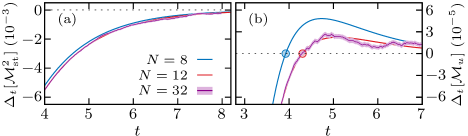
Figure 1: Mpemba effect. Evolution of $\Delta_{t}[\mathcal{A}]$ for the observables $\mathcal{A}=\mathcal{M}_{\text{st}}^{2}$ (a), and $\mathcal{A}=\mathcal{M}_{\text{u}}$ (b). We show the results for N=8 (blue), N=12 (red), and N=32 (purple, with a lighter shade representing the error bars of the MC data). In panel (b), the time at which $\Delta_{t}[\mathcal{M}_{\text{u}}]$ changes sign is marked by a dot.

In Fig. 1(a) we see that there is no crossing for $\mathcal{M}_{\text{st}}^{2}$; this is expected as we have prepared our system so that $\mathbb{E}_{t}^{\text{h}}[\mathcal{M}_{\text{st}}^{2}]$ is exponentially accelerated w.r.t. $\mathbb{E}_{t}^{\text{c}}[\mathcal{M}_{\text{st}}^{2}]$. Hence, the negative sign in Fig. 1(a). On the other hand, in Fig. 1(b) we see a crossing similar to those displayed in Fig. 3 of the main text: there is ME for the observable $\mathcal{M}_{\text{u}}$.

III.2 Preheating for faster cooling

Figure 2: Preheating strategy for faster cooling. Evolution of $\delta_{t}[\mathcal{A}]$ for $\mathcal{A}=\mathcal{E}$ (a), and $\mathcal{A}=\mathcal{M}_{\text{u}}$ (b). Colors red and purple (resp. blue and green) denote that the protocol includes (resp. does not include) an initial quench at temperature $T_{q}$. We show data for $N=8$ (dashed lines), $N=12$ (solid lines), and $N=32$ (solid lines with a lighter shade representing the error bars of the MC data). Both panels show the expected speed-up for the preheating protocol, although in (a) the error bars for $N=32$ are rather large to draw a definitive conclusion.

In this section, we compare the one-step protocol against a two-step protocol. In the former, we start with system in equilibrium at temperature $T_{0}=4.15$, and we let this system evolve with a bath temperature $T_{\text{b}}=1$. In the latter, we start again at $T_{0}$, but we first let the system to evolve with a bath at temperature $T_{q}=2000$ up to $t=t_{\text{w}}=0.156$; at this time, we put the system instantaneously in contact with a another bath at temperature $T_{\text{b}}=1$. We expect that this second preheating protocol will make the system to evolve faster than the standard one-step protocol. It is now useful to define $\delta_{t}[\mathcal{A}]=|\mathbb{E}_{t}[\mathcal{A}]-\mathbb{E}^{T_{\text{b}}}[\mathcal{A}]|/N$.

Figure 2 shows that preheating speeds up the evolution of the two observables not reported in the main text, namely $\mathcal{A}\in\{\mathcal{E},\mathcal{M}_{\text{u}}\}$. For the energy, this behavior is clear for the exact data ($N=8,12$), but for $N=32$ the results after $t\approx 6.5$ are less definitive due to the large error bars of the MC results.

III.3 Heating and cooling may be asymmetric processes

Here we will compare the behavior of starting at $T=T_{\text{A}}$ and evolving to the bath temperature $T=T_{\text{B}}$ against the inverse process: i.e. starting at $T=T_{\text{B}}$ and evolving to the bath temperature $T=T_{\text{A}}$. We have made two experiments: one with $T_{\text{A}}=1$ and $T_{\text{B}}=4.15\approx T_{\text{b}}^{*}$ (see left panels in Fig. 3), and the other one with $T_{\text{A}}=15.177$ and $T_{\text{B}}=4.15$ (see right panels in Fig. 3). Here $T_{\text{b}}^{*}$ is the temperature at which the staggered susceptibility $\chi_{\text{st}}$ attains a maximum [see Fig. 2(a) of the main text].

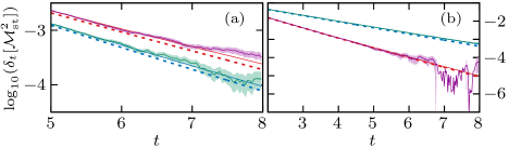
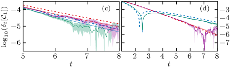
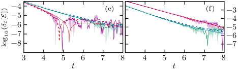
Figure 3: (A)symmetry in heating and cooling. Evolution of $\delta_{t}[\mathcal{A}_{\text{u}}]$ for $\mathcal{A}=\mathcal{M}_{\text{st}}^{2}$ (a,b), $\mathcal{A}=\mathcal{C}_{1}$ (c,d), and $\mathcal{A}=\mathcal{E}$ (e,f). In each panel, we depict cooling (blue and green) and heating (red and purple) processes. We show data for $N=8$ (dashed lines), $N=12$ (solid lines), and $N=32$ (solid lines with a lighter shade representing the errors of the MC data). The cooling and heating processes were carried out between: (a,c,e) $T_{A}=1$ and $T_{B}=4.15$; and (b,d,f) $T_{A}=15.177$ and $T_{B}=4.15$. For $\mathcal{M}_{\text{st}}^{2}$ and $\mathcal{C}_{1}$, it is slower to approach $T_{B}=4.15$: i.e. to heat-up in (a,c), and to cool-down in (b,d). However, the behavior is the opposite for the energy (e,f).

In Fig. 3 we show the data not reported in the main text, and corresponding to the observables $\mathcal{A}\in\{\mathcal{M}_{\text{st}}^{2},\mathcal{C}_{1},\mathcal{E}\}$ in panels (a,b), (c,d), and (e,f), respectively. Note that in panel (d), we observe a change of sign at $t\approx 2.5$ in the quantity $\mathbb{E}_{t}[\mathcal{C}_{1}]-\mathbb{E}^{T_{\text{b}}=T_{B}}[\mathcal{C}_{1}]$ for the system originally at $T_{A}=15.177$. We also observe such a change of sign in panel (e) for the quantity $\mathbb{E}_{t}[\mathcal{E}]-\mathbb{E}^{T_{\text{b}}=T_{B}}[\mathcal{E}]$ at $t\approx 5$ for the system originally at $T_{\text{A}}=1$.

We observe in Fig. 3(a,b,c,d), as we did in the main text for the observable $\mathcal{M}_{\text{u}}$, that for observables $\mathcal{M}_{\text{st}}^{2}$ and $\mathcal{C}_{1}$, it is always faster to move away from $T_{B}=4.15$ and approach $T_{\text{A}}$: i.e. to cool-down in (a,c), and to heat-up in (b,d).

However the behavior for the energy $\mathcal{E}$ is the opposite [see Fig. 3(e,f)]: it is faster to approach $T_{B}=4.15$: i.e. to heat-up in (e) and to cool-down in (f). The explanation of this effect was already given in the main text: for bath temperatures close to $T_{\text{B}}=4.15\approx T_{\text{b}}^{*}$, the coefficient $\beta_{2}^{\mathcal{E}}\approx 0$ [cf. Eq. (22)].

References

• Sokal [1997] A. D. Sokal, In Functional Integration: Basics and Applications (1996 Cargèse School), edited by C. DeWitt-Morette, P. Cartier and A. Folacci (Plenum, NY, 1997).
• Levin and Peres [2017] D. A. Levin and Y. Peres, Markov chains and mixing times, Vol. 107 (American Mathematical Soc., 2017).
• Note [1] Our definition of lazy dynamics is a generalization of the definition introduced in Sec. 1.3 of Ref. [2].
• Bortz et al. [1975] A. B. Bortz, M. H. Kalos,  and J. L. Lebowitz, J. Comp. Phys. 17, 10 (1975).
• Gillespie [1977] D. T. Gillespie, J. Phys. Chem. 81, 2340 (1977).
• Note [2] For complex observables, one would modify Eq. (1) as 𝒜|=\sum@\slimits@𝒙Ωπ𝒙Tb𝒜(𝒙)¯(𝒙),inner-product𝒜\sum@subscript\slimits@𝒙Ωsuperscriptsubscript𝜋𝒙subscript𝑇b¯𝒜𝒙𝒙\langle\,\mathcal{A}\,|\,\mathcal{B}\,\rangle=\sum@\slimits@_{\boldsymbol{x}\in\Omega}\,\pi_{\boldsymbol{x}}^{T_{\text{b}}}\,\overline{\mathcal{A}(\boldsymbol{x})}\,\mathcal{B}(\boldsymbol{x})\,, where the over-line stands for complex conjugation.
• Note [3] The reverse statement is not true: stationary does not entail detailed balance.
• Note [4] For any square matrix, it is possible to find a basis of the vector space formed solely by left-eigenvectors if, and only if, it is also possible to find a basis of right-eigenvectors. Furthermore, the spectrum of left eigenvalues is identical to the spectrum of right eigenvalues.
• Note [5] Therefore, the approach to equilibrium means that ${\cal T}^{n}[\mathcal{A}]$ approaches $\mathbb{E}^{T_{\text{b}}}[\mathcal{A}]\bm{1}$ as $n$ grows. In other words, after many time steps, the expected value for $\mathcal{A}$ becomes the equilibrium expectation value at temperature $T_{\text{b}}$, irrespective of the starting configuration $\bm{x}$.