Reconfigurable elastic neuromorphic metasurfaces towards mechanical intelligence and cognitive wave-based computing

Abstract

The ability of mechanical systems to perform basic computations has gained traction over recent years, providing an unconventional alternative to digital computing in off grid, low power, and severe thermal environments which render the majority of electronic components inoperable. However, much of the work in mechanical computing has focused on logic operations via quasi-static prescribed displacements in origami, bistable, and soft deformable matter. In here, we present a first attempt to describe the fundamental framework of an elastic neuromorphic metasurface that performs distinct classification tasks, providing a new set of challenges given the complex nature of elastic waves with respect to scattering and manipulation. Multiple layers of reconfigurable waveguides are phase-trained via constant weights and trainable activation functions in a manner that enables the resultant wave scattering at the readout location to focus on the correct class within the detection plane. We demonstrate the neuromorphic system’s ability to exhibit high accuracy in two distinct tasks owing to a fully reconfigurable design, eliminating the need for costly remanufacturing.

I   Introduction

Mechanical computing [1], a research field older than electronic computing, has gained a lot of interest over the past few years. Despite the limited capabilities of mechanical computers, the ability to integrate accurate computational and morphological capabilities with minimal energy requirements in a self-contained mechanical structure remains invaluable [2]. In the absence of digital access, resulting from power outages, extreme temperatures which render electronic components dysfunctional, ionizing radiation which trigger leakage currents between circuits, or the inability to accommodate forests of cables and hard-wired systems, a mechanical system’s capacity to recover a partial degree of computational ability is both prudent and critical, despite the understandable trade-off in computational pace and precision. The recent surge in mechanical computing research is equally motivated by new and transformative technologies requiring rapid (yet simple) data processing, and directly encoded autonomy and intelligence [3]. The latter presents an opportunity to exploit the dynamic behavior of structures, and capitalize on certain synergies associated with physical phenomena such as material response, deformation, and scattering to accomplish effective computation with minimal resources [4]. In keeping with these needs, several concepts have recently emerged with the goal of realizing mechanical systems capable of combinational logic, Boolean operations, and basic mathematics, using for example conductive polymers [5, 6] or bistable spring-mass chains [7, 8] that propagate mechanical signals when triggered. In tandem, there have been reports of origami-inspired metamaterials in which shear and expansion responses along different directions change the configuration state [9, 10, 11], and snap-through mechanisms where elastic instabilities and frictionless transitions are exploited to enable the creation of logic gates [12].

However, in pursuit of systems capable of learning and adaptation, the notions of neural networks and reservoir computing in the mechanical domain (often referred to as morphological computing [13]) have arguably gained even more traction. Ranging from binary-stiffness beams which learn desired shape-morphing behaviors [14], to Hopf oscillators [15, 16] and multi-stable metamaterials [17], there has been a spurt of activity demonstrating mechanical learning via programmable structures at different length scales. Inspired by neuromorphic sensors and electronics [18, 19], platforms mimicking the intricate workings of the brain and nervous system, the interplay of chemical and electronic impulses to relay vital information, and employing physical artificial neurons to perform computations, have found impetus in a broad range of applications and devices [20, 21], often exhibiting unparalleled compliance and energy efficiency [22]. Recognizing the power of wave scattering and propagation in multi-layered structures, even in the untrained state [23, 24], to perform basic mathematical operations in analog form, opens the door for robust, higher-order computations with the implementation of advanced learning schemes. Whether in the optical [25, 26, 27, 28, 29, 30, 31] or acoustic [32, 33] domains, tunable metasurfaces exploiting Snell refractions to tune and steer incident loads have been effectively utilized to conduct broad operations spanning differentiation, integration, and convolution, by correlating the waveform of an output to an input from the same physical domain, without resorting to learning algorithms.

Seeking to push the current boundary, we present in this work a class of neuromorphic metasurfaces which instills a level of cognitive intelligence in a multi-layered elastic classifier, enabling it to mechanically execute different computational tasks via a fully reconfigurable architecture. In the domain of analog wave-based computing, neuromorphic inference is rooted in the trained wave behavior of a set of metasurfaces comprised of tunable unit cells (physical neurons). The metasurfaces, spaced along the direction of wave propagation, form the basis of a neural network, and the subsequent wave scattering of a physical agent (e.g., light) in each of the physical layers constitutes the interactions within these layers [34, 35]. A readout mechanism is then used to interpret the results culminating in a desired output. While recent advances have been made in the development of such wave-based neuromorphic computers for photonic and electromagnetic applications [36, 37, 38, 39, 40], much less has been accomplished in the realm of mechanics. In here, we present a first attempt to describe the fundamental framework of a vibrational neuromorphic metasurface, capitalizing on the faster speeds of elastic waves in solids (compared to acoustic waves in air cavities [41]), but providing a new set of challenges given the complex nature of elastic waves with respect to scattering and manipulation. In addition to such challenges, current neuromorphic metasurfaces across different physical domains remain largely confined to passive designs which remain unchanged during operation. This not only constrains their operational frequency range but also limits their computational capabilities to the single task for which it is trained. We demonstrate the inner-workings of multiple layers of reconfigurable waveguides, which are phase-trained via constant weights and trainable activation functions in a manner that enables the resultant wave scattering at the readout location to focus on the correct class label within the detection plane. A bottom-up framework detailing the theory behind the unit cell, waveguide array, and overall metasurface designs is provided, and is then used to reconstruct the classic MNIST digit recognition classification problem using custom tailored hyperparameters of the proposed system. Finally, shifting from the MNIST to the Iris dataset, we demonstrate the neuromorphic system’s ability to reconfigure and retain high accuracy in two distinct tasks, forgoing reconstruction and eliminating the need for costly manufacturing adjustment.

II   Neuromorphic metasurface

II.1 Operational theory

We present an elastic neuromorphic metasurface composed of 3 sections: input gates, metasurface neurons, and detection units. These are equivalent to the input, hidden, and output layers of a digital neural network, respectively. The system can be excited at the input gates via any excitational signal which can be encoded into a vibrational waveform (e.g., noise, image, or dynamic load), culminating in elastic waves which propagate through the medium encompassing the metasurface layers. In current applications, the phase profile of a metasurface can be designed using an appropriate delay law to focus or steer a wavefront in a given direction. In this work, however, we will show the ability of a neuromorphic metasurface to generate a desirable output from a given input via intelligent, interlayer wave scattering. Provided with a set of tunable degrees of freedom (in this case, phase gradients between neighboring metasurface cells), the neuromorphic system trains itself to attain an intricate configuration of meta-neurons which allow the fully-assembled elastic structure to execute the required task.

While the model shown here takes inspiration from digital neural networks, its architecture is notably different in important ways, in order to accommodate the nuanced mechanics of elastic wave propagation. A conventional digital neural network is comprised of trainable weights and biases between the network layers. However, the activation function applied at each layer is typically non-trainable. In a neuromorphic metasurface, we will show that such weights represent wave scattering characteristics which are constrained functions of the chosen geometry, inertial, and stiffness properties. Once specified, these weights remain unchanged and are, therefore, non-trainable. Instead, phase delays within the metasurface layers provide an alternative tunable (and thus trainable) platform, shown to be analogous to a trainable activation function in a neural network framework.

II.2 Unit cell

Driven by the need for a mechanically-tunable system, we utilize a reconfigurable locally resonant unit cell which exhibits subwavelength scattering. Since computational pace is directly proportional to the wave speed in the medium, the focus here is on axial vibrations of the resonator given the higher speed of longitudinal wave propagation compared to flexural waves. The unit cell shown in Fig. 1b is designed to have effective properties, $m_{e}$ and $k_{e}$, equivalent to these of a lumped parameter model (Fig. 1a), which can be retrieved from finite element simulations of the actual cell designs. For the lumped parameter system shown in Fig. 1a, a transfer matrix $\mathbf{T}$ can be used to map the transmission from one end to the other via:

$$\begin{bmatrix}u_{3}\\ f_{3}\end{bmatrix}=\mathbf{T}\begin{bmatrix}u_{1}\\ f_{1}\end{bmatrix}$$ (1)

where $u_{1,3}$ and $f_{1,3}$ denote the displacement and forcing on the left and right boundaries, respectively. Subject to a harmonic excitation of frequency $\omega$, the steady-state equations of motion can be derived as:

$$-\omega^{2}m_{e}u_{2} =k_{e}(u_{1}+u_{3}-2u_{2})$$ (2a)

$$f_{1} =k_{e}(u_{2}-u_{1})$$ (2b)

$$f_{3} =k_{e}(u_{3}-u_{2})$$ (2c)

The four elements of $\mathbf{T}$ can be obtained by combining and rearranging Eqs. (1) and (2).

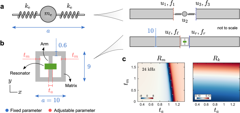
Figure 1: Unit cell design. (a) Lumped parameter representation. $m_{e}$ and $k_{e}$ are the effective mass and stiffness, respectively, and $a$ is the lattice constant. Right inset shows an elastic waveguide housing the spring-mass unit cell to determine the components of the transfer function, as detailed in Eq. (2). (b) Equivalent realization of the unit cell as a solid continuum. Blue and red dimensions represent fixed and adjustable parameters. Right inset shows corresponding waveguide used to compute the components of the transfer function, as detailed in Eq. (3). (c) Effective mass and stiffness ratios, $R_{m}$ and $R_{k}$, as functions of $t_{a}$ and $t_{m}$ as retrieved from the waveguide in (b) at $24$ kHz. Schematic diagrams are not drawn to scale and all dimensions are in mm.

The unit cell shown in Fig. 1b is composed of an Aluminum matrix ($E=70$ GPa, $\rho=2700$ kg/m³ and $\nu=0.33$), a Brass resonator ($E=97$ GPa, $\rho=8490$ kg/m³ and $\nu=0.31$) and two slender Aluminum beams (resonator arms) which attach the resonator to the matrix. These arms are placed along the $y$-axis, perpendicular to the longitudinal deformation of the unit cell along the $x$-direction, enabling a coupling between the bending modes of the resonator arms and the axial vibrations of the unit cell. Similar to Eq. (1), the transfer matrix $\mathbf{T}$ can be used to relate the state vector $[u_{r}~{}f_{r}]^{T}$ on the right side to that on the left side $[u_{\ell}~{}f_{\ell}]^{T}$ of the unit cell, where $u_{\ell,r}$ and $f_{\ell,r}$ can be computed from a finite element model (FEM) as follows:

$$u_{\ell,r} =\frac{1}{a}\int_{0}^{a}u(x=[0,a],y)dy$$ (3a)

$$f_{\ell,r} =\frac{A}{a}\int_{0}^{a}\sigma(x=[0,a],y)dy$$ (3b)

In Eq. (3), $u$ denotes the $x$-component of the unit cell’s displacement, $a$ is the length (lattice constant), $\sigma$ is the axial stress, and $A$ is the cross-sectional area which is a product of length and plate thickness. An equivalent lumped parameter system would thus need to satisfy:

$$m_{e} =\frac{{f_{\ell}}^{2}-{f_{r}}^{2}}{\omega^{2}(f_{\ell}u_{r}+f_{r}u_{\ell})}$$ (4a)

$$k_{e} =\frac{f_{r}+f_{\ell}}{u_{r}-u_{\ell}}$$ (4b)

allowing $m_{e}$ and $k_{e}$ to be calculated from Eqs. (3) and (4) using force and displacement data retrieved from the FEM.

At the core of the neuromorphic metasurface concept is the ability to achieve full phase tunability over a $2\pi$ range while maintaining high transmission within the waveguide, as will be detailed in the next section. The unit cell, therefore, needs to be reconfigurable in order to admit different values of $m_{e}$ and $k_{e}$ as needed. The effective widths of the resonator arm $t_{a}$ and the vertical section of the unit cell matrix $t_{m}$, both indicated on Fig. 1b, play a central role in the bending stiffness of both parts. Thus, changes in these two parameters significantly alter the dynamics of the unit cell described by $m_{e}$ and $k_{e}$. Control over these effective widths can be exercised via a 3D realization of the unit cell with rotating arms having rectangular cross-sections, as shown in Fig. 2c and successfully implemented in literature [42]. We define the effective mass and stiffness ratios as $R_{m}=m_{e}/m_{\text{slab}}$ and $R_{k}=k_{e}/k_{\text{slab}}$, respectively, where $m_{\text{slab}}=\rho Aa$ and $k_{\text{slab}}=EA/[a(1-\nu^{2})]$ denote the mass and axial stiffness, respectively, of an aluminum slab of the same size. Figure 1c depicts the variation of $R_{m}$ and $R_{k}$ as functions of $t_{a}$ and $t_{m}$ at a frequency of $24$ kHz. The behavior shows that while both thicknesses affect both effective ratios (i.e., mass and stiffness), $R_{m}$ and $R_{k}$ are observed to be largely dependent on $t_{a}$ and $t_{m}$, respectively.

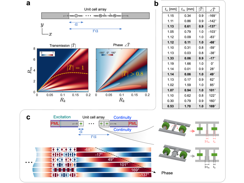
Figure 2: Waveguide scattering. (a) Transmission amplitude $|\bar{T}|$ and phase $\angle\bar{T}$ for a waveguide comprised of $r=6$ unit cells. $R_{k}$ and $R_{m}$ denote the effective stiffness and mass ratios, respectively. The dashed line in $|\bar{T}|$ indicates a full transmission scenario ($|\bar{T}|=1$), while the mask in $\angle\bar{T}$ represents $|\bar{T}|>0.8$ regions. (b) Waveguides generated using $R_{k,m}$ and $\bar{T}$ maps in order to exhibit high transmission at 20^∘ phase differences (covering a 360^∘ range). (c) Wave steering achieved using an assembly of the six highlighted waveguides in (b) via finite element modeling. The top panel depicts the details of the numerical simulations showing locations of continuity boundary conditions and the perfectly matched layer (PML). Shown on the right is a 3D physical realization of the reconfigurable waveguide design exploiting the change in bending stiffness for rotating cross sections to achieve the sought tunability.

II.3 Scattering and waveguide design

The scattering properties of a waveguide of $r$ unit cells can be evaluated starting with the dispersion relation, which can be derived as follows:

$$m_{e}\omega^{2}=2k_{e}\sin^{2}(\frac{\kappa a}{2})$$ (5)

where $\kappa=\omega/c$ is the wave number in the propagation direction and $\omega$ is the angular frequency of the harmonic wave. The transmission coefficient $\bar{T}$ can be computed from:

$$\bar{T}=\frac{2}{2\cos{(r\kappa a)}+\mathrm{i}(zz_{s}^{-1}+z_{s}z^{-1})\sin{(r\kappa a)}}$$ (6)

where $\mathrm{i}=\sqrt{-1}$, $z=\rho Ac$ is the mechanical impedance, and $c=\sqrt{E/[\rho(1-\nu^{2})]}$ is the axial wave speed. The system’s characteristic impedance $z_{s}$ can be defined as:

$$z_{s}=\frac{\sqrt{\frac{m_{e}k_{e}}{2}}}{\cos{(\frac{\kappa a}{2})}}$$ (7)

For a waveguide consisting of $r=6$ unit cells, we start by considering a wide range of $m_{e}$ and $k_{e}$ values, and obtain $\kappa$ from Eq. (5). This is then used to determine the corresponding $z_{s}$ via Eq. (7), allowing the transmission amplitude $|\bar{T}|$ and phase $\angle\bar{T}$ to be evaluated by using Eq. (6), as shown in Fig. 2a. A high transmission ($|\bar{T}|>0.8$) mask is applied to the phase map to facilitate the selection of $R_{k}$ and $R_{m}$ combinations that maintain a minimum acceptable transmission at a given phase. For detailed derivations of the equations used in this section, the reader is referred to Ref. [43].

As will become evident later, the neuromorphic metasurface needs to maintain sufficient tunability for good training and subsequent performance. We utilize the unit cell design shown in Fig. 1b as the building block of one-dimensional arrays (see Fig. 2c) which can impose a full range of time delay over $2\pi$ phase, while maintaining high transmission. Making use of $R_{k,m}$ (Fig. 1c) and the transmission amplitude and phase maps (Fig. 2a), eighteen arrays are generated with intervals of approximately $20^{\circ}$ phase difference as summarized in the table provided in Fig. 2b. A steering waveguide is assembled from six select cases from the table, and the resultant displacement field is demonstrated in Fig. 2c for validation. Finally, in the culminating neuromorphic metasurface, each unit cell array in the metasurface is treated as a singular point, neglecting lateral propagating waves. As such, the Aluminum slabs are chosen to be $1$ mm thicker than the array itself to mitigate vertical interactions that are unaccounted for and ensure isolation from adjacent arrays.

II.4 Metasurface neural architecture

The neuromorphic metasurface architecture consists of four consecutive layers: an input layer, two metasurface layers, and an output layer, as illustrated in Fig. 3a. Each waveguide is comprised of an array of $r=6$ unit cells, henceforth referred to as a “meta-neuron”. For a given classification dataset, training and test samples with $K$ features are reshaped into a single dimensional vector with the same number of elements. This vector is then fed to the elastic medium in the form of $K$ displacement point sources at the input layer. At the far side of the neuromorphic metasurface (output layer), a set of $N$ detection units are defined corresponding to the $N$ labels of the classification problem. For a successful mechanical neural network, the goal of the training is to distinctly engineer the two metasurface layers such that for a given input (i.e., test sample) generating a distinct excitation pattern stemming from the $K$ point sources constituting this input, the scattered elastic wavefronts would predominantly focus on the appropriate detection unit spatially corresponding to the correct $N$ label.

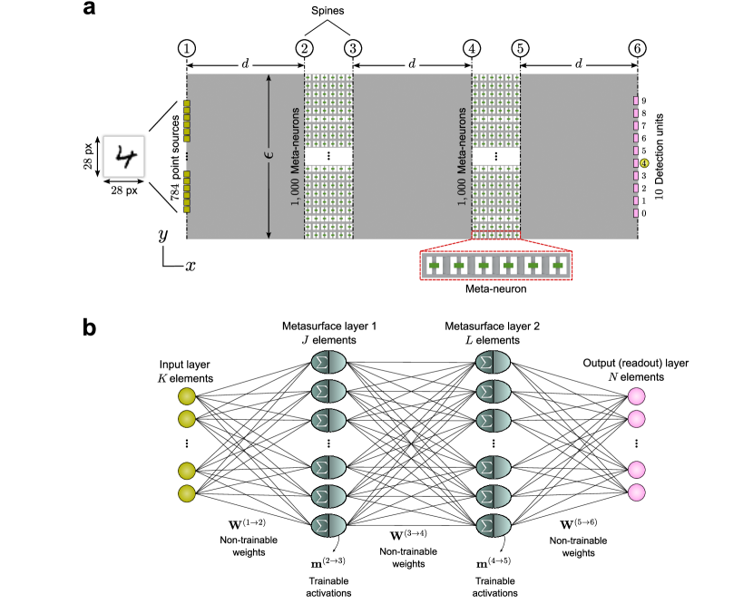
Figure 3: Reconfigurable elastic neuromorphic metasurface. (a) Schematic illustration of the assembled neuromorphic system for the MNIST digit recognition task. Six vertical cross sections, referred to as spines and labeled $1$ through $6$, define the different mechanical components. Spines $1$ and $6$ mark the input and output (readout) layers, with $K=784$ sources and $N=10$ detection units. Two metasurface layers span the regions between spines $2\to 3$ and $4\to 5$ each housing $J=L=1,000$ meta-neurons. Each meta-neuron consists of $6$ identical unit cells and retains a unique design based on tuned values of $t_{a}$ and $t_{m}$, culminating in $2,000$ distinctly different meta-neurons. Regions before, between, and after the metasurface layers are homogenous aluminum plates providing an elastic medium for the guided interlayer wave scattering shown in the three wavefield segments of Fig. 4a. (b) Logic diagram depicting the neural architecture of the elastic neuromorphic system, emphasizing the non-trainable weights $\mathbf{W}^{(1\rightarrow 2)}$, $\mathbf{W}^{(3\rightarrow 4)}$, and $\mathbf{W}^{(5\rightarrow 6)}$, as well as the trainable activation functions $\mathbf{m}^{(2\rightarrow 3)}$ and $\mathbf{m}^{(4\rightarrow 5)}$. All layers are dense.

To develop the analytical framework, we evaluate wave propagation amplitudes at the six spines labeled $1$ through $6$ in Fig. 3a, representing the beginning and end of different layers of interest. The region $1\to 2$ hosts elastic waves emanating from $K$ point excitations at the input layer and propagating through a homogenous medium, until arriving at $J$ meta-neurons at the first metasurface layer. Since each point source generates a harmonic planar wave in a thin elastic substrate, a circular wave approximation is employed to describe the outward-propagating wavefronts as follows [44]:

$$u^{(2)}_{j,k}(t)=\frac{u^{(1)}_{k}}{\sqrt{|\mathbf{p}^{(2)}_{j}-\mathbf{p}^{(1)}_{k}|}}e^{\mathrm{i}(\kappa({|\mathbf{p}^{(2)}_{j}-\mathbf{p}^{(1)}_{k}|})-\omega t)}$$ (8)

where $u^{(2)}_{j,k}(t)$ represents the $x$-component of displacement right before meta-neuron $j$ at spine $2$, as a result of point source $k$ at spine $1$, while $\mathbf{p}^{(2)}_{j}$ and $\mathbf{p}^{(1)}_{k}$ denote the position vectors of the $j^{\text{th}}$ meta-neuron and the $k^{\text{th}}$ point source, respectively. As can be inferred from Eq. (8), the displacement amplitude $u^{(2)}_{j,k}(t)$ is directly proportional to the source amplitude $u^{(1)}_{k}$, but inversely proportional to the square root of the euclidean distance $|\mathbf{p}^{(2)}_{j}-\mathbf{p}^{(1)}_{k}|$. The net displacement at the $j^{\text{th}}$ meta-neuron as a result of all the sources at the input layer can be computed via superposition as follows:

$$u^{(2)}_{j}(t)=\sum^{K}_{k=1}\frac{u^{(1)}_{k}}{\sqrt{|\mathbf{p}^{(2)}_{j}-\mathbf{p}^{(1)}_{k}|}}e^{\mathrm{i}(\kappa({|\mathbf{p}^{(2)}_{j}-\mathbf{p}^{(1)}_{k}|})-\omega t)}$$ (9)

Based on this formulation, the wave propagation weights $w^{(1\rightarrow 2)}_{j/k}$ between the $k^{\text{th}}$ source point on spine $1$ and the $j^{\text{th}}$ meta-neuron on spine $2$ can be defined as the factor multiplied by the amplitude of each point source, and therefore involves the effects of medium size and properties on the wave emerging from this source to the corresponding meta-neuron, such that:

$$w^{(1\rightarrow 2)}_{j/k}=\frac{e^{\mathrm{i}\kappa({|\mathbf{p}^{(2)}_{j}-\mathbf{p}^{(1)}_{k}|})}}{\sqrt{|\mathbf{p}^{(2)}_{j}-\mathbf{p}^{(1)}_{k}|}}$$ (10)

The entire process can be collectively cast in matrix from using $\mathbf{u}^{(2)}=\mathbf{W}^{(1\rightarrow 2)}\mathbf{u}^{(1)}$, where $\mathbf{u}^{(2)}=[u^{(2)}_{1}u^{(2)}_{2}\dots u^{(2)}_{J}]^{T}$, $\mathbf{u}^{(1)}=[u^{(1)}_{1}u^{(1)}_{2}\dots u^{(1)}_{K}]^{T}$, and the wave propagation matrix from spine 1 to 2 is defined as follows:

$$\mathbf{W}^{(1\rightarrow 2)}=\begin{bmatrix}w^{(1\rightarrow 2)}_{1/1}&w^{(1\rightarrow 2)}_{1/2}&.&.&.&w^{(1\rightarrow 2)}_{1/K}\\ w^{(1\rightarrow 2)}_{2/1}&w^{(1\rightarrow 2)}_{2/2}&.&.&.&w^{(1\rightarrow 2)}_{2/K}\\ .&.&.&&&.\\ .&.&&.&&.\\ .&.&&&.&.\\ w^{(1\rightarrow 2)}_{J/1}&w^{(1\rightarrow 2)}_{J/2}&.&.&.&w^{(1\rightarrow 2)}_{J/K}\\ \end{bmatrix}$$ (11)

Upon reaching the first metasurface layer, each meta-neuron transmits the incident wave with an amplitude adjustment and a phase shift, as detailed in section IIC. As a result, the metasurface layer can be thought of as a black box with an impact mathematically described as a complex exponential of the applied phase shift multiplied by the corresponding transmission coefficient. As a result, the displacements at spine $3$ can be described as $\mathbf{u}^{(3)}=\mathbf{m}^{(2\rightarrow 3)}\odot\mathbf{u}^{(2)}$, where $\odot$ denotes element-wise multiplication and

$$\mathbf{m}^{(2\rightarrow 3)}=\begin{bmatrix}t_{1}^{(2\rightarrow 3)}e^{\mathrm{i}\phi_{1}^{(2\rightarrow 3)}}\\ t_{2}^{(2\rightarrow 3)}e^{\mathrm{i}\phi_{2}^{(2\rightarrow 3)}}\\ .\\ .\\ .\\ t_{J}^{(2\rightarrow 3)}e^{\mathrm{i}\phi_{J}^{(2\rightarrow 3)}}\end{bmatrix}$$ (12)

is the metasurface modulation vector from spine $2$ to $3$ with elements $t_{j}^{(2\rightarrow 3)}$ and $e^{\mathrm{i}\phi_{j}^{(2\rightarrow 3)}}$ corresponding to the transmission and phase imposed by the $j^{\text{th}}$ meta-neuron, respectively. Note that $t_{j}^{(2\rightarrow 3)}$ is dependent on $\phi_{j}^{(2\rightarrow 3)}$ for any given waveguide as demonstrated in Fig. 2b, a factor which will be taken into consideration during the training process in the next section. The wave propagation scheme from spine $3$ to $4$ is almost identical to that from $1$ to $2$, with a slight modification based on the Huygens-Fresnel principle [45]:

$$u^{(4)}_{l,j}(t)=-\frac{\mathrm{i}}{2\lambda}\frac{\epsilon}{J}\frac{u^{(3)}_{j}(t)}{\sqrt{|\mathbf{p}^{(4)}_{l}-\mathbf{p}^{(3)}_{j}|}}e^{\mathrm{i}(\kappa(|\mathbf{p}^{(4)}_{l}-\mathbf{p}^{(3)}_{j}|)-\omega t)}$$ (13)

where $u^{(4)}_{l,j}(t)$ indicates the displacement right before the $l^{\text{th}}$ meta-neuron at spine $4$, as a result of the assumed point source $j$ at spine $3$. In Eq. (13), $\epsilon$ refers to the width of the metasurface, while $\lambda$ denotes the wavelength of the propagating wave. Following the same notation as before, $\mathbf{p}^{(4)}_{l}$ and $\mathbf{p}^{(3)}_{j}$ mark the position vectors of the $l^{\text{th}}$ and $j^{\text{th}}$ meta-neurons at spines $4$ and $3$, respectively. As a result, the wave propagation weights from spine $3$ to $4$ can be derived as follows:

$$w^{(3\rightarrow 4)}_{l/j}=-\frac{\mathrm{i}}{2\lambda}\frac{\epsilon}{J}\frac{e^{\mathrm{i}(\kappa|\mathbf{p}^{(4)}_{l}-\mathbf{p}^{(3)}_{j}|)})}{\sqrt{|\mathbf{p}^{(4)}_{l}-\mathbf{p}^{(3)}_{j}|}}$$ (14)

and, similarly, the wave propagation profile in matrix form is given by $\mathbf{u}^{(4)}=\mathbf{W}^{(3\rightarrow 4)}\mathbf{u}^{(3)}$, where

$$\mathbf{W}^{(3\rightarrow 4)}=\begin{bmatrix}w^{(3\rightarrow 4)}_{1/1}&w^{(3\rightarrow 4)}_{1/2}&.&.&.&w^{(3\rightarrow 4)}_{1/J}\\ w^{(3\rightarrow 4)}_{2/1}&w^{(3\rightarrow 4)}_{2/2}&.&.&.&w^{(3\rightarrow 4)}_{2/J}\\ .&.&.&&&.\\ .&.&&.&&.\\ .&.&&&.&.\\ w^{(3\rightarrow 4)}_{L/1}&w^{(3\rightarrow 4)}_{L/2}&.&.&.&w^{(3\rightarrow 4)}_{L/J}\\ \end{bmatrix}$$ (15)

with $\mathbf{W}^{(3\rightarrow 4)}$ representing the wave propagation matrix from spine $3$ to $4$, and $w^{(3\rightarrow 4)}_{l/j}$ representing the elements of this matrix corresponding to the wave propagation weight from a virtual source $j$ to a meta-neuron $l$. Following the process outlined in the first metasurface layer and Eq. (12), the wave propagation scheme in the second metasurface layer can be likewise derived as $\mathbf{u}^{(5)}=\mathbf{m}^{(4\rightarrow 5)}\odot\mathbf{u}^{(4)}$, in which:

$$\mathbf{m}^{(4\rightarrow 5)}=\begin{bmatrix}t_{1}^{(4\rightarrow 5)}e^{\mathrm{i}\phi_{1}^{(4\rightarrow 5)}}\\ t_{2}^{(4\rightarrow 5)}e^{\mathrm{i}\phi_{2}^{(4\rightarrow 5)}}\\ .\\ .\\ .\\ t_{L}^{(4\rightarrow 5)}e^{\mathrm{i}\phi_{L}^{(4\rightarrow 5)}}\end{bmatrix}$$ (16)

is the metasurface modulation vector from spine $4$ to $5$ with elements $t_{l}^{(4\rightarrow 5)}$ and $e^{\mathrm{i}\phi_{l}^{(4\rightarrow 5)}}$ corresponding to the transmission and phase imposed by the $l^{\text{th}}$ meta-neuron, respectively. Finally, the wave propagation scheme at the back end of the neuromorphic metasurface can be evaluated via $\mathbf{u}^{(6)}=\mathbf{W}^{(5\rightarrow 6)}\mathbf{u}^{(5)}$, where $\mathbf{W}^{(5\rightarrow 6)}$ is the wave propagation matrix from spine $5$ to $6$ (output layer).

The output layer at spine $6$ is virtually divided into $N$ equidistant and equally-long detection units corresponding to the $N$ labels of the classification problem. This is done by breaking the displacement vector $\mathbf{u}^{(6)}$ (which includes a number of points significantly larger than that of the classification labels) into $N$ smaller vectors $\mathbf{u}^{(6)}_{[n]}$, with $n$ ranging from $1$ to $N$. As a result, the wave energy focused on the $n^{\text{th}}$ detection unit can be calculated as ${|\mathbf{u}^{(6)}_{[n]}|}^{2}={\mathbf{u}^{(6)}_{[n]}}^{*}\cdot\mathbf{u}^{(6)}_{[n]}$, where $(\bullet)^{*}$ is the complex conjugate. Once a test sample is fed at spine $1$ and undergoes the multi-layer scattering described herein, the energies at all the detection units of spine $6$ are quantitatively compared, and the unit corresponding to the largest value is reported as the label corresponding to the input, as chosen by the elastic neuromorphic classifier.

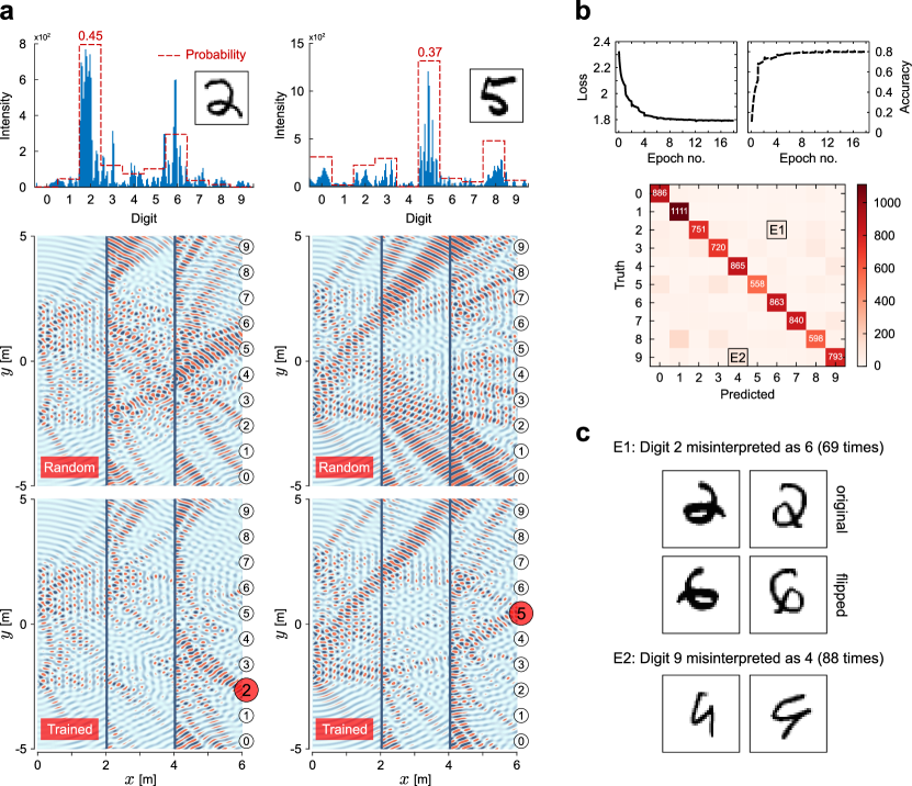
Figure 4: Performance of the elastic neuromorphic metasurface. (a) Output of the neuromorphic metasurface for two digit recognition test samples from the MNIST dataset corresponding to the digits “$2$” (left) and “$5$” (right). The top row shows the intensities (blue bars) and probabilities (red dashed lines) at different detection units within the output (readout) layer. Bottom and middle rows show the scattered wavefields for trained and randomly initialized neuromorphic metasurfaces, respectively. (b) Classification accuracy (right) and model loss (left) for the training dataset, and confusion matrix (bottom) for the testing dataset. The training dataset is divided into 27 batches processed at each epoch. (c) Examples of erroneous recognition: “$2$” and “$9$” misinterpreted as “$6$” and “$4$”, respectively, due to subtle shape similarities, corresponding to the E1 and E2 markings on the confusion matrix in (b).

III   Training

A conventional neural network is mathematically described by:

$$\mathbf{y}^{(i+1)}=f(\mathbf{b}^{(i+1)}+\mathbf{W}^{(i\rightarrow i+1)}\mathbf{y}^{(i)})$$ (17)

where $\mathbf{y}^{(i)}$ is a vector of values assigned to neurons in the $i^{\text{th}}$ layer, $\mathbf{W}^{(i\rightarrow i+1)}$ is the weights matrix, and $\mathbf{b}^{(i+1)}$ is the bias. The architecture of the elastic neuromorphic system is similar to the above framework in that $\mathbf{y}^{(i)}$ is analogous to the displacement vector $\mathbf{u}^{(i)}$ and the weights matrix $\mathbf{W}^{(i\rightarrow i+1)}$ is equivalent to the wave propagation matrix from one spine to the next. Furthermore, the activation function $f$ is analogous to the metasurface effect inflicted by $\mathbf{m}^{(i\rightarrow i+1)}$ vector on the incident wave. However, the bias $\mathbf{b}^{(i+1)}$ is not applicable in this study. More importantly, in the elastic neuromorphic system, the wave propagation matrices do not change once dimensions and material properties are finalized, rendering them hyperparameters, contrary to the weights of a digital neural network which are the primary trainable parameters throughout the learning process. Another stark contrast is the activation function applied at each layer of a digital neural network, which is typically identical for all neurons. In the elastic neuromorphic system, however, phase shifts applied by each meta-neuron of the metasurface layers (and consequently the $\mathbf{m}^{(i\rightarrow i+1)}$ vectors) are trainable parameters in the learning algorithm. The neuromorphic metasurface’s wave manipulation approach can be perceived as multiple beam-forming segments combined together in one line and steering separate parts of the incident wave.

For illustration, and without loss of generality, we tackle a digit recognition problem using the MNIST dataset. Each (training or test) sample in the dataset consists of a $28\times 28$ matrix of gray-scale pixel intensities. The matrix is flattened into a 1D vector of $784$ elements, and the pixel intensities are used as displacement amplitudes for $K=784$ excitation point sources at the input layer. At the far end of the neuromorphic metasurface (output layer), $N=10$ detection units are defined corresponding to the digit labels $0$ to $9$. The metasurface layers are set to be $d=2$ m apart with $J=L=1,000$ meta-neurons in each metasurface layer (Size and dimensions of the elastic neuromorphic metasurface are scalable, and can be up- or downsized depending on target application and operational frequency). The distance between neighboring point sources at the input layer is set to $10$ mm, equal to the width of a single meta-neuron. The model is developed in TensorFlow using custom Keras layers and is trained in Python. The flattened input samples are cast into a vector of complex numbers $\mathbf{u}^{(1)}_{784\times 1}$ since the weights and the phase shift have to be complex in order to retain the displacement components from one layer to another. Two custom dense layers are then defined in the model for the two metasurface layers, with non-trainable weights ($\mathbf{W}^{(1\rightarrow 2)}_{1000\times 784}$ and $\mathbf{W}^{(3\rightarrow 4)}_{1000\times 1000}$ from Eqs. (11) and (15), respectively), no biases, and custom activation functions ($\mathbf{m}^{(2\rightarrow 3)}_{1000\times 1}$ and $\mathbf{m}^{(4\rightarrow 5)}_{1000\times 1}$ from Eqs. (12) and (16), respectively). As explained earlier, the dependency of $t_{j}^{(2\rightarrow 3)}$ on $\phi_{j}^{(2\rightarrow 3)}$ for each meta-neuron is also considered while applying the activation functions in the training process. Lastly, an additional custom dense layer is defined as the output layer with non-trainable weights ($\mathbf{W}^{(5\rightarrow 6)}_{1000\times 1000}$) and with no biases. In this final layer, the well-known Softmax activation function is implemented.

The learning is carried out using $60,000$ training samples and a $10\%$ split for validation. The Sparse Categorical Cross-entropy loss function, which is highly effective in multi-class classification problems, is adopted, and the Adam optimizer is employed to improve the training performance via a defined learning rate schedule. After training, the model is evaluated using $10,000$ (blind) test samples to report its accuracy. Upon ensuring that the training has been executed with high efficacy, the trained metasurface vectors $\mathbf{m}^{(i\rightarrow i+1)}$ are used alongside Fig. 2b to determine the corresponding design parameters $t_{a}$ and $t_{k}$ for each and every meta-neuron.

IV   Performance and results

The training scheme is performed by an Intel Xeon^® Gold 6230 CPU @ $2.10$ GHz and a RAM of 128 GB, running on Microsoft Windows 10. Figure 4a showcases the output of the neuromorphic metasurface for two digit recognition samples corresponding to the digits “$2$” and “$5$”. The top row illustrates the distribution of intensity ${|\mathbf{u}^{(6)}_{[n]}|}^{2}$ and probability over the output layer at different detection units. The latter is computed as the ratio of the summation of point intensities at the detection units to the total intensity of the output layer. As evident from these plots, the neuromorphic metasurface is able to successfully classify these samples. The shown wavefields at the bottom of Fig. 4a further corroborate this by depicting the wave scattering through the different layers of the neuromorphic metasurface from the input location at spine $1$ to the output (readout) location at spine $6$. The displacements in each of the three sections shown ($1\to 2$, $3\to 4$, and $5\to 6$) are individually normalized with respect to the same section for better visualization. The middle row of Fig. 4a displays the wavefield resulting from a randomized, untrained design, further confirming the effectiveness of the trained wave scattering.

The top panel of Fig. 4b summarizes the loss and accuracy as functions of the epoch number. We select $10$ epochs with an accuracy of $80$%, which take $53$ minutes of training on the reported PC. Beyond the two examples shown, the overall performance is evaluated using a confusion matrix for the trained model based on its performance on the entire testing dataset, as demonstrated in the bottom panel of Fig. 4b. While this provides important insights into the model’s capability of correctly classifying the tested samples, it also helps identify potential areas of improvement, such as recognizing specific digit shapes that may be challenging to accurately predict. As a case in point, the labels E1 and E2 marked on the confusion matrix correspond to erroneous recognition of the digits “$2$” and “$9$” as $6$ and $4$, respectively, due to subtle shape similarities illustrated in Fig. 4c.

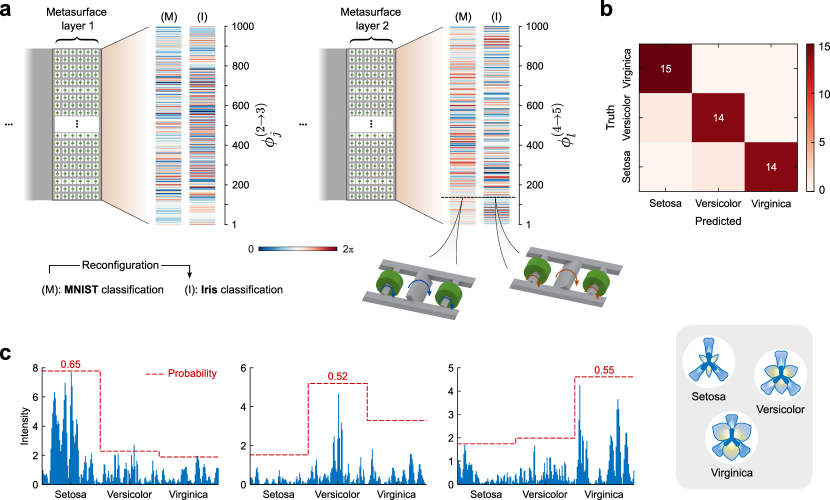
Figure 5: Reconfigurability. (a) Change in the phase profile of the 1,000 meta-neurons in the first (left) and second (right) metasurface layers following training as the neuromorphic system switches from the MNIST (M) to the Iris (I) classification task. (b) Confusion matrix generated from the testing data depicting the system’s accuracy in the Iris problem. (c) Intensities (blue bars) and probabilities (red dashed lines) at the three detection units within the output layer for input samples corresponding to, from left to right, Setosa, Versicolor, and Virginica.

V   Discussion

V.1 Hyperparameters

The computational accuracy of the elastic neuromorphic metasurface is affected by several hyperparameters that, if adequately tuned, can considerably improve several performance metrics. These are aspects which are set at the design stage and control the learning process, as opposed to being derived via training. The contribution of each of these to the overall classification accuracy is evaluated by individually altering parameters of interest while holding the rest unchanged from the values reported earlier, as shown in Table 1. It is important to acknowledge that, for efficiency purposes, the model used in these studies is trained for a predetermined number of epochs, reaching a near-stabilized accuracy level, while the training duration may be shorter compared to the main model.

Table 1: Effect of different hyperparameters stated in the left column of the table on the overall classification accuracy. Cases typed in boldface refer to the main model defined in Sec. III.

No. of Layers	2	3	4	5
	80.4%	86.1%	88.7%	88.5%
Distance between Layers	1 m	2 m	3 m	4 m
	78.1%	80.4%	81.4%	76.7%
No. of Neurons	300	700	1,000	2000
	63.1%	74.8%	80.4%	79.5%
Detection Units Width	0.3 m	0.7 m	1 m	1.2 m
	82.1%	80.8%	80.4%	80.6%
Training Metric	Intensity		Displacement
	80.4%		75.5%
Digit Processing	Gray-scale		Binary
	80.4%		73.6%

As can be inferred from the first row of Table 1, increasing the number of metasurface layers improves the accuracy in a proportional manner. A similar trend is observed for both the distance between layers $d$ and the number of neurons in each layer ($J$ or $L$). Nonetheless, a trade-off between accuracy and practicality is unavoidable. Accuracy gains become insignificant beyond a certain range while the structural size multiplies, detrimentally influencing wave intensity at the detection units, which, in turn, adversely affects the accuracy as noted in the last column. Contrarily, reducing the dimensions of the detection units marginally enhances the accuracy which, while appearing advantageous, concurrently permits a substantial portion of the energy to be redirected away from these units, resulting in low intensities at the detection layer.

As evident from the fifth row of Table 1, employing the intensity of the wavefield at the output layer ${|\mathbf{u}^{(6)}_{[n]}|}^{2}$ as the evaluation metric yields improved accuracy compared to the displacement. Finally, although the utilization of binary simplifications for the sample digit pixels at the input layer could offer more flexibility in fabrication and testing, allowing on/off actuation, reducing the number of sources through combination, and eliminating the need for amplitude adjustment at the excitation location, it is observed that a gray-scale representation leads to a slightly improved accuracy, as can be seen in the last row of Table 1.

V.2 Reconfigurability

It is critically important to note that in addition to being scarce, physical neural networks developed to date, even those deployed in non-mechanical domains including photonics [34, 36] and acoustics [41], have not yet overcome the need to reconstruct their core wave-scattering components in order to retrain and carry out a different task. Owing to their inability to alter trainable nodes post design, the computational capacity of such systems remains limited to executing the single computational task that the constitutive cells were optimized for. Motivated by the need to overcome this drawback, we demonstrate here the ability of the elastic neuromorphic metasurface to exercise an unprecedented degree of reconfigurability, allowing it to cater to distinct classification tasks, forgoing reconstruction and eliminating the need for costly remanufacturing. To illustrate, we re-utilize the baseline model generated for MNIST digit recognition and retrain it without changing any of its hyperparameters to execute the Iris flower classification task [46]. The new task involves the binning of Iris flower samples into three distinct classes (Setosa, Versicolor, and Virginica) based on four features: sepal length, sepal width, petal length, and petal width. The values of these features represent the amplitudes of four excitation point sources placed at the input layer (i.e., $K=4$), each two separated by $1.5$ m. The number of meta-neurons in the two metasurface layers is kept at $J=L=1,000$, while $N=3$ detection units corresponding to the three classes are defined at the output (readout) layer. The model is trained on $70\%$ of the available dataset ($105$ samples) and tested on the remaining $30\%$, yielding an accuracy of $97\%$ and $96\%$ for the training and testing datasets, respectively.

Figure 5a shows the precise phase profiles for all $1,000$ meta-neurons in the first (Spine $2\to 3$) and second (Spine $4\to 5$) metasurface layers for both the originally trained (MNIST, or M) and retrained (Iris, or I) datasets. The small insets reveal the phase reconfiguration of the metasurface unit cell via resonator arm rotation, effectively switching the trainable meta-neurons from (M) to (I). Figure 5b shows the confusion matrix for the 3 classes of the Iris dataset generated from the testing data. Furthermore, we show the intensity (blue bars) and probability (red dashed lines) distribution over the three detection units within the output (readout) layer in Fig. 5c, confirming the neuromorphic system’s robust ability to relearn a diverse set of tasks, with high accuracy and within the same mechanical platform.

VI   Conclusions

In this work, the foundation of wave-based neuromorphic computing has been introduced to the field of structural mechanics, utilizing guided in-plane vibrational waves in an elastic substrate. Edge excitations depicting the features of an input sample from two distinct multivariate datasets were fed to the neuromorphic system in the form of an array of spatially equidistant mechanical monopoles. These excitations were made to propagate through multiple layers of trained waveguides, eventually focusing the bulk portion of scattered wave intensity on the correct label identifier on a prescribed detection plane. Exploiting analogies between the different components of the proposed neuromorphic assembly and neural architectures, a customized neural network was defined accounting for non-trainable, constant wave propagation matrices (weights) and trainable phase delays (activation functions). Owing to the inherent reconfigurable nature of the physical meta-neurons within the metasurface arrays, the proposed system represents an embodiment of wave-based analog computers which is no longer constrained to a single unaltered task, and one where neurons can mechanically recompose their local phase profile to adapt to a new training scheme and execute a new task, on demand and with no trade offs in performance accuracy.

References

- Yasuda et al. [2021] H. Yasuda, P. R. Buskohl, A. Gillman, T. D. Murphey, S. Stepney, R. A. Vaia, and J. R. Raney, Nature 598, 39–48 (2021).
- Zangeneh-Nejad et al. [2021] F. Zangeneh-Nejad, D. L. Sounas, A. Alù, and R. Fleury, Nature Reviews Materials 6, 207 (2021).
- Riley et al. [2022] K. S. Riley, S. Koner, J. C. Osorio, Y. Yu, H. Morgan, J. P. Udani, S. A. Sarles, and A. F. Arrieta, Advanced Intelligent Systems 4, 2200158 (2022).
- [4] “Darpa nature as computer (nac) program,” https://www.darpa.mil/program/nature-as-computer.
- El Helou et al. [2021] C. El Helou, P. R. Buskohl, C. E. Tabor, and R. L. Harne, Nature Communications 12 (2021).
- El Helou et al. [2022] C. El Helou, B. Grossmann, C. E. Tabor, P. R. Buskohl, and R. L. Harne, Nature 608, 699–703 (2022).
- Ion et al. [2017] A. Ion, L. Wall, R. Kovacs, and P. Baudisch, in Proceedings of the 2017 CHI Conference on Human Factors in Computing Systems, CHI ’17 (Association for Computing Machinery, New York, NY, USA, 2017) p. 977–988.
- Bilal et al. [2017] O. R. Bilal, A. Foehr, and C. Daraio, Proceedings of the National Academy of Sciences 114, 4603 (2017).
- Treml et al. [2018] B. Treml, A. Gillman, P. Buskohl, and R. Vaia, Proceedings of the National Academy of Sciences 115, 6916 (2018).
- Meng et al. [2021] Z. Meng, W. Chen, T. Mei, Y. Lai, Y. Li, and C. Chen, Extreme Mechanics Letters 43, 101180 (2021).
- Liu et al. [2023a] Z. Liu, H. Fang, J. Xu, and K.-W. Wang, Advanced Intelligent Systems 5, 2200146 (2023a).
- Mei et al. [2021] T. Mei, Z. Meng, K. Zhao, and C. Q. Chen, Nature Communications 12 (2021).
- Lee et al. [2022] R. H. Lee, E. A. Mulder, and J. B. Hopkins, Science Robotics 7 (2022).
- Hopkins et al. [2023] J. B. Hopkins, R. H. Lee, and P. B. Sainaghi, Smart Materials and Structures (2023).
- Shougat et al. [2021] M. R. E. U. Shougat, X. Li, T. Mollik, and E. Perkins, Scientific Reports 11, 19465 (2021).
- Shougat et al. [2022] M. R. E. U. Shougat, X. Li, and E. Perkins, Physical Review E 105, 044212 (2022).
- Liu et al. [2023b] Z. Liu, H. Fang, J. Xu, and K.-W. Wang, arXiv preprint arXiv:2305.19856 (2023b).
- Sarkar et al. [2022] T. Sarkar, K. Lieberth, A. Pavlou, T. Frank, V. Mailaender, I. McCulloch, P. W. Blom, F. Torricelli, and P. Gkoupidenis, Nature Electronics 5, 774 (2022).
- Gkoupidenis [2022] P. Gkoupidenis, Nature Electronics 5, 721 (2022).
- Li et al. [2018] Y. Li, Z. Wang, R. Midya, Q. Xia, and J. J. Yang, Journal of Physics D: Applied Physics 51, 503002 (2018).
- van De Burgt et al. [2018] Y. van De Burgt, A. Melianas, S. T. Keene, G. Malliaras, and A. Salleo, Nature Electronics 1, 386 (2018).
- Xia and Yang [2019] Q. Xia and J. J. Yang, Nature materials 18, 309 (2019).
- Silva et al. [2014] A. Silva, F. Monticone, G. Castaldi, V. Galdi, A. Alù, and N. Engheta, Science 343, 160 (2014).
- Wright et al. [2022] L. G. Wright, T. Onodera, M. M. Stein, T. Wang, D. T. Schachter, Z. Hu, and P. L. McMahon, Nature 601, 549 (2022).
- Wan et al. [2021] L. Wan, D. Pan, T. Feng, W. Liu, and A. A. Potapov, Frontiers of Optoelectronics 14, 187 (2021).
- Pors et al. [2015] A. Pors, M. G. Nielsen, and S. I. Bozhevolnyi, Nano letters 15, 791 (2015).
- Zhou et al. [2020] Y. Zhou, W. Wu, R. Chen, W. Chen, R. Chen, and Y. Ma, Advanced Optical Materials 8, 1901523 (2020).
- Cordaro et al. [2019] A. Cordaro, H. Kwon, D. Sounas, A. F. Koenderink, A. Alù, and A. Polman, Nano letters 19, 8418 (2019).
- Bao et al. [2020] L. Bao, R. Y. Wu, X. Fu, and T. J. Cui, Annalen der Physik 532, 2000069 (2020).
- Wan et al. [2020] L. Wan, D. Pan, S. Yang, W. Zhang, A. A. Potapov, X. Wu, W. Liu, T. Feng, and Z. Li, Optics Letters 45, 2070 (2020).
- Zhou et al. [2021a] J. Zhou, H. Qian, J. Zhao, M. Tang, Q. Wu, M. Lei, H. Luo, S. Wen, S. Chen, and Z. Liu, National science review 8 (2021a).
- Zuo et al. [2018] S.-Y. Zuo, Y. Tian, Q. Wei, Y. Cheng, and X.-J. Liu, Journal of Applied Physics 123, 091704 (2018).
- Zuo et al. [2022] S. Zuo, C. Cai, X. Li, Y. Tian, and E. Liang, Journal of Physics D: Applied Physics 55, 354001 (2022).
- Wu et al. [2020] Z. Wu, M. Zhou, E. Khoram, B. Liu, and Z. Yu, Photonics Research 8, 46 (2020).
- Ballarini et al. [2020] D. Ballarini, A. Gianfrate, R. Panico, A. Opala, S. Ghosh, L. Dominici, V. Ardizzone, M. De Giorgi, G. Lerario, G. Gigli, et al., Nano Letters 20, 3506 (2020).
- Fu et al. [2023] T. Fu, Y. Zang, Y. Huang, Z. Du, H. Huang, C. Hu, M. Chen, S. Yang, and H. Chen, Nature Communications 14, 70 (2023).
- Zhou et al. [2021b] T. Zhou, X. Lin, J. Wu, Y. Chen, H. Xie, Y. Li, J. Fan, H. Wu, L. Fang, and Q. Dai, Nature Photonics 15, 367 (2021b).
- Léonard et al. [2021] F. Léonard, A. S. Backer, E. J. Fuller, C. Teeter, and C. M. Vineyard, ACS Photonics 8, 2103 (2021).
- Léonard et al. [2022] F. Léonard, E. J. Fuller, C. M. Teeter, and C. M. Vineyard, Optics Express 30, 12510 (2022).
- Lio and Ferraro [2021] G. E. Lio and A. Ferraro, in Photonics, Vol. 8 (MDPI, 2021) p. 65.
- Weng et al. [2020] J. Weng, Y. Ding, C. Hu, X.-F. Zhu, B. Liang, J. Yang, and J. Cheng, Nature communications 11, 6309 (2020).
- Attarzadeh et al. [2020] M. Attarzadeh, J. Callanan, and M. Nouh, Physical Review Applied 13, 021001 (2020).
- Lee et al. [2018] H. Lee, J. K. Lee, H. M. Seung, and Y. Y. Kim, Journal of the Mechanics and Physics of Solids 112, 577 (2018).
- Giurgiutiu [2007] V. Giurgiutiu, Structural health monitoring: with piezoelectric wafer active sensors (Elsevier, 2007).
- Goodman [2005] J. Goodman, Introduction to Fourier Optics, McGraw-Hill physical and quantum electronics series (W. H. Freeman, 2005).
- Fisher [1936] R. A. Fisher, Annals of eugenics 7, 179 (1936).