Understanding CNN Hidden Neuron Activations Using Structured Background Knowledge and Deductive Reasoning

Abstract

A major challenge in Explainable AI is in correctly interpreting activations of hidden neurons: accurate interpretations would provide insights into the question of what a deep learning system has internally detected as relevant on the input, demystifying the otherwise black-box character of deep learning systems. The state of the art indicates that hidden node activations can, in some cases, be interpretable in a way that makes sense to humans, but systematic automated methods that would be able to hypothesize and verify interpretations of hidden neuron activations are underexplored.

In this paper, we provide such a method and demonstrate that it provides meaningful interpretations. Our approach is based on using large-scale background knowledge – approximately 2 million classes curated from the Wikipedia concept hierarchy – together with a symbolic reasoning approach called Concept Induction based on description logics, originally developed for applications in the Semantic Web field. Our results show that we can automatically attach meaningful labels from the background knowledge to individual neurons in the dense layer of a Convolutional Neural Network through a hypothesis and verification process.

1 Introduction

Deep learning has led to significant advances in artificial intelligence applications including image classification (Ramprasath, Anand, and Hariharan 2018), speech recognition (Graves and Jaitly 2014), translation (Auli et al. 2013), drug design (Segler et al. 2018), medical diagnosis (Choi et al. 2019), climate sciences (Liu et al. 2016), and many more. Despite these successes, the black-box nature of deep learning systems remains problematic for some application areas, especially those involving automated decisions and safety-critical systems. For example, Apple co-founder Steve Wozniak accused Apple of gender discrimination, claiming that the new Apple Card gave him a credit limit that was ten times higher than that of his wife even though the couple shares all property (Hamilton 2019). In an image search, only 11% of the top image results for “CEOs” were images of women despite the fact that women make up 27% of US CEOs (Silberg and Manyika 2019). Other application areas of particular concern include safety-critical systems such as self-driving cars (Chen and Huang 2017), drug discovery and treatment recommendations (Rifaioglu et al. 2020; Hariri and Narin 2021), and others, as deep learning systems are prone to adversarial attacks, e.g., by altering classification results by introducing adversarial examples (Bau et al. 2020) or simply controlling the order in which training images are presented (Shumailov et al. 2021). Some of these attacks are difficult or impossible to detect after the fact (Goldwasser et al. 2022; Clifford et al. 2022).

Standard assessments of deep learning performance consist of statistical evaluation, but do not seem sufficient to address these shortcomings as they cannot provide reasons or explanations for particular system behaviors (Doran, Schulz, and Besold 2018). Consequently, it remains very important to develop strong explanation methods for deep learning systems. While there has been significant progress on this front (see Section 2), the current state of the art is mostly restricted to explanation analyses based on a relatively small number of predefined explanation categories. This is problematic from a principled perspective, as this relies on the assumption that explanation categories pre-selected by humans would be viable explanation categories for deep learning systems – an as-yet unfounded conjecture. Other state of the art explanation systems rely on modified deep learning architectures, usually leading to a decrease in system performance compared to unmodified systems (Zarlenga et al. 2022). Ideally, we would want strong explanation capabilities while maintaining the underlying learning architecture.

In this paper, we address the aforementioned shortcomings by using Concept Induction, i.e., formal logical deductive reasoning (Lehmann and Hitzler 2010). We show that our approach can indeed provide meaningful explanations for hidden neuron activation in a Convolutional Neural Network (CNN) architecture for image scene classification (on the ADE20K dataset (Zhou et al. 2019)), using a class hierarchy consisting of about $2\cdot 10^{6}$ classes, derived from Wikipedia, as the pool of categories (Sarker et al. 2020). The benefits of our approach to explainable deep learning are: (a) it can be used on unmodified and pre-trained deep learning architectures, (b) it assigns semantic categories (i.e., class labels expressed in formal logic) to hidden neurons such that images related to these labels activate the corresponding neuron with high probability, and (c) it can construct these labels from a very large pool of categories.

The rest of this paper is organized as follows. Section 2 discusses related work on explainable deep learning. Section 3 presents our approach. Section 4 provides evaluation results and Section 5 discussions thereof. Section 6 concludes and discusses follow-up research directions. A technical appendix provides more complete details of our experiments and results. Source code, input data, raw result files, and parameter settings for replication are available online.

2 Related Work

Explaining (interpreting, understanding, justifying) automated AI decisions has been explored from the early 1970s. With the recent advances in deep learning (LeCun, Bengio, and Hinton 2015), its wide usage in nearly every field, and its opaque nature make explainable AI more important than ever, and there are multiple ongoing efforts to demystify deep learning (Gunning et al. 2019; Adadi and Berrada 2018; Minh et al. 2022). Existing explainable methods can be categorized based on input data (feature) understanding, e.g., feature summarizing (Selvaraju et al. 2016; Ribeiro, Singh, and Guestrin 2016), or based on the model’s internal unit representation, e.g., node summarizing (Zhou et al. 2018; Bau et al. 2020). Those methods can be further categorized as model-specific (Selvaraju et al. 2016) or model-agnostic (Ribeiro, Singh, and Guestrin 2016). Another kind of approach relies on human interpretation of explanatory data returned, such as counterfactual questions (Wachter, Mittelstadt, and Russell 2017).

We focus on the understanding of internal units of the neural network-based deep learning models. Given a deep learning model and its prediction, we ask the questions “What does the deep learning model’s internal unit represent? Are those units activated by human-understandable concepts?” Prior work has shown that internal units may indeed represent human-understandable concepts (Zhou et al. 2018; Bau et al. 2020), but these approaches require semantic segmentation (Xiao et al. 2018) (which is time- and compute-expensive) or explicit concept annotations (Kim et al. 2018) (which are expensive to acquire). To get around these limitations, we take a different approach by using a hypothesis generation and validation approach based on Concept Induction analysis for hypothesis generation (details in Section 3). The use of large-scale description logic background knowledge means that we draw explanations from a very large pool of explanation categories.

There has been some work using knowledge graphs to produce explanations from deep learning models (Confalonieri et al. 2021; Díaz-Rodríguez et al. 2022), and also on using Concept Induction to provide explanations (Sarker et al. 2017; Procko et al. 2022), but they focused on analysis of input-output behavior, i.e., on generating an explanation for the overall system. We focus instead on the different task of understanding internal (hidden) node activations.

To the best of our knowledge, our use of Concept Induction with large-scale background knowledge as pool for explanation generation (to understand the internal node activations) is novel. Furthermore our method (training, Concept Induction analysis, and verification) is fully automateable without the need for human intervention.

3 Approach

In this section we detail our technical approach. Section 3.1 covers the scene recognition scenario that we use to present our approach; Section 3.2 describes the technical components used for explanation generation; Section 3.3 presents our results and how we obtain label hypotheses for hidden node activations (with examples); and Section 3.4 details the label hypothesis validation process and results. Experimental evaluation can be found in Section 4. More details regarding our experimental parameters are in Appendix A.

3.1 Preparations: Scenario and CNN Training

We use a scene classification from images scenario to demonstrate our approach, drawing from the ADE20K dataset (Zhou et al. 2019) which contains more than 27,000 images over 365 scenes, extensively annotated with pixel-level objects and object part labels. The annotations are not used for CNN training, but rather only for generating label hypotheses that we will describe in Section 3.3.

Architectures	Training acc	Validation acc
Vgg16	80.05%	46.22%
InceptionV3	89.02%	51.43%
Resnet50	35.01%	26.56%
Resnet50V2	87.60%	86.46%
Resnet101	53.97%	53.57%
Resnet152V2	94.53%	51.04%

Table 1: Performance (accuracy) of different architectures on the ADE20K dataset. The system we used, based on performance, is bolded.

We train a classifier for the following scene categories: “bathroom,” “bedroom,” “building facade,” “conference room,” “dining room,” “highway,” “kitchen,” “living room,” “skyscraper,” and “street.” We weigh our selection toward scene categories which have the highest number of images and we deliberately include some scene categories that should have overlapping annotated objects – we believe this makes the hidden node activation analysis more interesting. We did not conduct any experiments on any other scene selections yet, i.e., we did not change our scene selections based on any preliminary analyses.

We trained a number of CNN architectures in order to use the one with highest accuracy, namely Vgg16 (Simonyan and Zisserman 2015), InceptionV3 (Szegedy et al. 2016) and different versions of Resnet – Resnet50, Resnet50V2, Resnet101, Resnet152V2 (He et al. 2016a, b). Each neural network was fine-tuned with a dataset of 6,187 images (training and validation set) of size 224x224 for 30 epochs with early stopping to avoid overfitting. We used Adam as our optimization algorithm, with a categorical cross-entropy loss function and a learning rate of 0.001.

We select Resnet50V2 because it achieves the highest accuracy (see Table 1). Note that for our investigations, which focus on explainability of hidden neuron activations, achieving a very high accuracy for the scene classification task is not essential, but a reasonably high accuracy is necessary when considering models which would be useful in practice.

3.2 Preparations: Concept Induction and Background Knowledge

For label hypotheses generation, we make use of Concept Induction (Lehmann and Hitzler 2010) which is based on deductive reasoning over description logics, i.e., over logics relevant to ontologies, knowledge graphs, and generally the Semantic Web field (Hitzler, Krötzsch, and Rudolph 2010; Hitzler 2021). Concept Induction has indeed already been shown, in other scenarios, to be capable of producing labels that are meaningful for humans inspecting the data (Widmer et al. 2022). A Concept Induction system accepts three inputs: (1) a set of positive examples $P$, (2) a set of negative examples $N$, and (3) a knowledge base (or ontology) $K$, all expressed as description logic theories, and all examples $x\in P\cup N$ occur as instances (constants) in $K$. It returns description logic class expressions $E$ such that $K\models E(p)$ for all $p\in P$ and $K\not\models E(q)$ for all $q\in N$. If no such class expressions exist, then it returns approximations for $E$ together with a number of accuracy measures.

For scalability reasons, we use the heuristic Concept Induction system ECII (Sarker and Hitzler 2019) together with a background knowledge base that consists only of a hierarchy of approximately 2 million classes, curated from the Wikipedia concept hierarchy and presented in (Sarker et al. 2020). We use coverage as accuracy measure, defined as

$$\textrm{coverage}(E)=\frac{|Z_{1}|+|Z_{2}|}{|P\cup N|},$$

where $Z_{1}=\{p\in P\mid K\models E(p)\}$ and $Z_{2}=\{n\in N\mid K\not\models E(n)\}$. $P$ is the set of all positive instances, $N$ is the set of all negative instances, and $K$ is the knowledge base provided to ECII as part of the input.

For the Concept Induction analysis, positive and negative example sets will contain images from ADE20K, i.e., we need to include the images in the background knowledge by linking them to the class hierarchy. For this, we use the object annotations available for the ADE20K images, but only part of the annotations for the sake of simplicity. More precisely, we only use the information that certain objects (such as windows) occur in certain images, and we do not make use of any of the richer annotations such as those related to segmentation. All objects from all images are then mapped to classes in the class hierarchy using the Levenshtein string similarity metric (Levenshtein 1975) with edit distance $0$. For example, the ADE20K image ADE_train_00001556.jpg has “door” listed as one of the objects shown, which is mapped to the “door” concept of the Wikipedia concept hierarchy. Note that the scene information is not used for the mapping, i.e., the images themselves are not assigned to specific (scene) classes in the class hierarchy – they are connected to the hierarchy only through the objects that are shown (and annotated) in each image.

3.3 Generating Label Hypotheses

The general idea for generating label hypotheses using Concept Induction is as follows: given a hidden neuron, $P$ is a set of inputs (i.e., in this case, images) to the deep learning system that activate the neuron, and $N$ is a set of inputs that do not activate the neuron (where $P$ and $N$ are the sets of positive and negative examples, respectively). As mentioned above, inputs are annotated with classes from the background knowledge for Concept Induction, but these annotations and the background knowledge are not part of the input to the deep learning system. ECII generates a label hypothesis for the given neuron on inputs $P$, $N$, and the background knowledge.

We first feed 1,370 ADE20K images to our trained Resnet50V2 and retrieve the activations of the dense layer. We chose to look at the dense layer because previous studies indicate (Olah, Mordvintsev, and Schubert 2017) that earlier layers of a CNN respond to low level features such as lines, stripes, textures, colors, while layers near the final layer respond to higher-level features such as face, box, road, etc. The higher-level features align better with the nature of our background knowledge.

The dense layer consists of 64 neurons. We chose to analyze each of the neurons separately. We are aware that activation patterns involving more than one neuron may also be informative in the sense that information may be distributed among several neurons, but the analysis of such activation patterns will be part of follow-up work.

For each neuron, we calculate the maximum activation value across all images. We then take the positive example set $P$ to consist of all images that activate the neuron with at least 80% of the maximum activation value, and the negative example set $N$ to consist of all images that activate the neuron with at most 20% of the maximum activation value (or do not activate it at all). The highest scoring response of running ECII on these sets, together with the background knowledge described in Section 3.2, is shown in Table 2 for each neuron, together with the coverage of the ECII response. For each neuron, we call its corresponding label the target label, e.g., neuron $0$ has target label “building.” Note that some target labels consist of two concepts, e.g., “footboard, chain” for neuron 49 – this occurs if the corresponding ECII response carries two class expressions joined by a logical conjunction, i.e., in this example “footboard $\sqcap$ chain” (as description logic expression) or $\textnormal{footboard}(x)\land\textnormal{chain}(x)$ expressed in first-order predicate logic.

Neuron #	Obtained Label(s)	Images	Coverage	Target %	Non-Target %
0	building	164	0.997	89.024	72.328
1	cross_walk	186	0.994	88.710	28.923
3	night_table	157	0.987	90.446	56.714
6	dishcloth, toaster	106	0.999	16.038	39.078
11	river_water	157	0.995	31.847	22.309
16	mountain, bushes	108	0.995	87.037	24.969
18	slope	139	0.983	92.086	69.919
22	skyscraper	156	0.992	99.359	54.893
26	skyscraper, river	112	0.995	77.679	35.489
30	teapot, saucepan	108	0.998	81.481	47.984
40	sculpture, side_rail	119	0.995	25.210	21.224
41	open_fireplace, coffee_table	122	0.992	88.525	16.381
43	central_reservation	157	0.986	95.541	84.973
46	casserole	157	0.999	45.223	36.394
48	road	167	0.984	100.000	73.932
49	footboard, chain	126	0.982	88.889	66.702
51	road, car	84	0.999	98.810	48.571
54	skyscraper	156	0.987	98.718	70.432
58	plank, casserole	80	0.998	3.750	3.925
63	edifice, skyscraper	178	0.999	92.135	48.761

Table 2: Selected representative data as discussed throughout the text (the full version is Table 4 in Appendix A). Images: Number of images used per label. Target %: Percentage of target images activating the neuron above 80% of its maximum activation. Non-Target %: The same, but for all other images. Bold denotes neurons whose labels are considered confirmed.

Let us take neuron 1 as a concrete example. After training, neuron 1 has a maximum activation value of 10.90, 80% of which is 8.72, and 20% of which is 2.18. The positive example set $P$ thus consist of all images activating the neuron with at least 8.72, and the negative example set $N$ consists of all images activating the neuron with at most 2.18. Example images are shown in Figure 1 middle top (positive) and bottom (negative). The top ranked ECII response on this input was “cross_walk,” with a coverage score of 0.994. (Note that some of the positive images may not actually have a crosswalk, like the top left and bottom right positive images shown in Figure 1 – we discuss this in Section 4.) We consider these target labels to be working hypotheses for activation triggers for the corresponding neuron. As hypotheses, they require further confirmation, i.e., some of these hypotheses may be rejected.

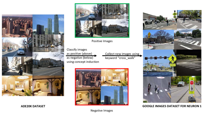
Figure 1: Example of images that were used for generating and confirming the label hypothesis for neuron 1.

3.4 Confirming Label Hypotheses

The process described in Section 3.3 produces label hypotheses for all neurons investigated. The next step is to confirm or reject these hypotheses by testing the labels with new images. We use each of the target labels to search Google Images with the labels as keywords (requiring responses to be returns for both keywords if the label is a conjunction of classes). We call each such image a target image for the corresponding label or neuron. We use Imageye to automatically retrieve the images, collecting up to 200 images that appear first in the Google Images search results, filtering for images in JPEG format (ADE20K images are in JPEG format) and with a minimum size of 224x224 pixels (again corresponding to ADE20K). For each retrieval label, we use 80% of the obtained images, reserving the remaining 20% for the statistical evaluation described in Section 4. The number of images used in the hypothesis confirmation step, for each label, is given in Table 2. These images are fed to the network to check (a) whether the target neuron (with the retrieval label as target label) activates, and (b) whether any other neurons activate.

The Target % column of Table 2 shows the percentage of the target images that activate each neuron to at least 80% of its maximum activation. Using neuron 1 as an example, 88.710% of the images retrieved with the label “cross_walk” activate the neuron ($\geq$ 80%). However, this neuron only activates only for 28.923% of these images, (indicated in the Non-Target % column) when presented with images retrieved using all other labels from Table 2 excluding “cross_walk.”

We define a target label for a neuron to be confirmed if it activates (with at least 80% of its maximum activation value) for at least 80% of its target images regardless of how much or how often it activates for non-target images (see Section 4 for the analysis of non-target activation). We use 80% as the cut-off for both neuron activation and label hypothesis confirmation – these are ad-hoc values that could both be chosen differently (we discuss this in Technical Appendix A.2). This cut-off value ensures strong association and responsiveness to images retrieved under the target label. We discuss the relevance of the Non-Target column in the next section.

Returning to neuron 1, we retrieve 233 new images with keyword “cross_walk,” 186 of which (80%) are used in this step. Example images are shown in Figure 1 to the right. 165 of these images (i.e., 88.710%) activate neuron 1 with at least 8.72 (which is 80% of its maximum activation value of 10.90). Since $88.710\geq 80$, we consider the label “cross_walk” confirmed for neuron 1. After this step, we arrive at a list of 20 confirmed labels listed in Table 3.

4 Statistical Evaluation

After generating the confirmed labels (as in Section 3), we statistically evaluate the node labeling using the remaining images from those retrieved from Google Images as described in Section 3.4. Results are shown in Table 3, omitting neurons that were not activated by any image, i.e., their maximum activation value was 0. The statistical evaluation shows that Concept Induction analysis with large-scale background knowledge yields meaningful labels that stably explain neuron activation.

Neuron #	Label(s)	Images	# Activations (%)		Mean		Median		z-score	p-value
			targ	non-t	targ	non-t	targ	non-t
0	building	42	80.95	73.40	2.08	1.81	2.00	1.50	-1.28	0.0995
1	cross_walk	47	91.49	28.94	4.17	0.67	4.13	0.00	-8.92	<.00001
3	night_table	40	100.00	55.71	2.52	1.05	2.50	0.35	-6.84	<.00001
8	shower_stall, cistern	35	100.00	54.40	5.26	1.35	5.34	0.32	-8.30	<.00001
16	mountain, bushes	27	100.00	25.42	2.33	0.67	2.17	0.00	-6.72	<.00001
18	slope	35	91.43	68.85	1.59	1.37	1.44	1.00	-2.03	0.0209
19	wardrobe, air_conditioning	28	89.29	65.81	2.30	1.28	2.30	0.84	-4.00	<.00001
22	skyscraper	39	97.44	56.16	3.97	1.28	4.42	0.33	-7.74	<.00001
29	lid, soap_dispenser	33	100.00	80.47	4.38	2.14	4.15	1.74	-5.92	<.00001
30	teapot, saucepan	27	85.19	49.93	2.52	1.05	2.23	0.00	-4.28	<.00001
36	tap, crapper	23	91.30	70.78	3.24	1.75	2.82	1.29	-3.59	<.00001
41	open_fireplace, coffee_table	31	80.65	15.11	2.03	0.14	2.12	0.00	-7.15	<.00001
43	central_reservation	40	97.50	85.42	7.43	3.71	8.08	3.60	-5.94	<.00001
48	road	42	100.00	74.46	6.15	2.68	6.65	2.30	-7.78	<.00001
49	footboard, chain	32	84.38	66.41	2.63	1.67	2.30	1.17	-2.58	0.0049
51	road, car	21	100.00	47.65	5.32	1.52	5.62	0.00	-6.03	<.00001
54	skyscraper	39	100.00	71.78	4.14	1.61	4.08	1.12	-7.60	<.00001
56	flusher, soap_dish	53	92.45	64.29	3.47	1.48	3.08	0.86	-6.47	<.00001
57	shower_stall, screen_door	34	97.06	32.31	2.60	0.61	2.53	0.00	-7.55	<.00001
63	edifice, skyscraper	45	88.89	48.38	2.41	0.83	2.36	0.00	-6.73	<.00001

Table 3: Evaluation details as discussed in Section 4. Images: Number of images used for evaluation. # Activations: (targ(et)): Percentage of target images activating the neuron (i.e., activation at least 80% of this neuron’s activation maximum); (non-t): Same for all other images used in the evaluation. Mean/Median (targ(et)/non-t(arget)): Mean/median activation value for target and non-target images, respectively.

We consider each neuron-label pair in each row in Table 3, e.g., for neuron 1, the hypothesis is that this neuron activates more strongly for images retrieved using the keyword “cross_walk” than for images retrieved using other keywords. The corresponding null hypothesis is that activation values are not different. Table 3 shows the 20 hypotheses to test, corresponding to the 20 neurons with confirmed labels – recall that a double label such as neuron 16’s “mountain, bushes” is treated as one label consisting of the conjunction of the two keywords.

There is no reason to assume that activation values would follow a normal distribution, or that the preconditions of the central limit theorem would be satisfied. We therefore base our statistical assessment on the Mann-Whitney U test (McKnight and Najab 2010) which is a non-parametric test that does not require a normal distribution. Essentially, by comparing the ranks of the observations in the two groups, the test allows us to determine if there is a statistically significant difference in the activation percentages between the target and non-target labels.

The resulting z-scores and p-values are shown in Table 3. Of the 20 null hypotheses, 19 are rejected at $p<0.05$, but most (all except neurons 0, 18 and 49) are rejected at much lower p-values. Only neuron 0’s null hypothesis could not be rejected. The Non-Target % column of Table 2 provides some insight into the results for neurons 0, 18 and 49: target and non-target values for these neurons are closer to each other – the difference is particularly small for neuron 0. Likewise, differences between target and non-target values for mean activation values and median activation values in Table 3 are smaller for these neurons. This hints at ways to improve label hypothesis generation or confirmation, and we will discuss this and other ideas for further improvement below under possible future work.

For our running example (neuron 1), we use the remaining 47 target images (20% of the 165 images retrieved during the label hypothesis confirmation step) for the statistical analysis. 43 of these images (91.49%) activate the neuron at $\geq$ 8.72 (80% of its maximum activation value of 10.90), with a mean and median activation of 4.17 and 4.13, respectively. Of all other images (non-target images) used in the evaluation (the sum of the numbers in the image column in Table 3 minus 47), only 28.94% activate neuron 1 at $\geq$ 8.72, for a mean of 0.67 and a median of 0.00. The Mann-Whitney U test yields a z-score of -8.92 and $p<0.00001$, thus rejecting the null hypothesis that activation values for target and non-target images are not different. In addition, the negative z-score indicates that the activation values for non-target images are indeed lower than for the target images. Figure 2 shows examples of target images that do not activate neuron 1 (left) and non-target images that do activate it (right).

The Mann-Whitney U results show that, for most neurons listed in Table 3 (with $p<0.00001$), activation values for target images are overwhelmingly higher than for non-target images. The negative z-scores with high absolute values informally indicate the same, as do the mean and median values. Neurons 16 and 49, for which the hypotheses also hold but with $p<0.05$ and $p<0.01$, respectively, still exhibit statistically significant higher activation values for target than for non-target images, but not overwhelmingly so. This can also be informally seen from lower absolute values of the z-scores, and from smaller differences between the means and the medians.

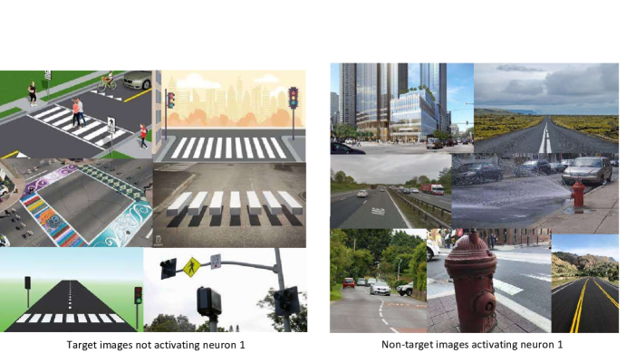
Figure 2: Examples of some Google images used: target images (“cross_walk”) that did not activate the neuron; non-target images from labels like “central_reservation,” “road and car,” and “fire_hydrant” that activated the neuron.

5 Discussion

While the statistical analysis clearly supports the viability of our approach as carried out, we can see from Table 3 that there is still significant activation of neurons by non-target images, leaving room for refinement. Ideally, we would be able to arrive at confirmed neuron labels where the number of non-target activations (Table 3, # Activations (%) non-t – column 5) is very low while the number of target activations (# Activations(%) targ – column 4) remains high. For example, neuron 16 is always activated by target images and is only activated by 25% of non-target images, meaning that we can use the neuron activation to predict (with relatively high certainty) whether or not mountains and bushes are in the image. In contrast, for neuron 29 – with a much higher non-target value – we can be much less certain if an image activating the neuron indeed contains lid and soap dispenser. High certainty, i.e., high target and low non-target values, would provide highly accurate explanations of system behavior. At the same time, however, the data collected during the label generation step, in particular that in the Target % and Non-Target % columns of Table 2, can already be used as a proxy for the certainty we can attach to a detection.

It is instructive to have another look at our example neuron 1. The images depicted on the left in Figure 2 – target images not activating the neuron – are mostly computer-generated as opposed to photographic images as in the ADE20K dataset. The lower right image does not actually show the ground at the crosswalk, but mostly sky and only indirect evidence for a crosswalk by means of signage, which may be part of the reason why the neuron does not activate. The right-hand images are non-target images that activate the neuron. We may conjecture that other road elements, prevalent in these pictures, may have triggered the neuron. We also note that several of these images show bushes or plants, which is particularly interesting because the ECII response with the third-highest coverage score is “bushes, bush” with a coverage score of 0.993 and 48.052% of images retrieved using this label actually activate the neuron (the second response for this neuron is also “cross_walk”).

Our results point to promising future research directions, including studying ensemble activation, analyzing different hidden layers, transfer to other application scenarios, and application to other deep learning architectures. Other possible avenues involve additional strengthening of our results including detailed analyses and exploration – and thus optimization – of parameters that were often chosen ad-hoc for this paper. We discuss some of them below, in sequence of appearance in the paper. Additional results along these lines can be found in Appendix A.

The choice of background knowledge – based on objects appearing in the images – was mostly one of convenience, as suitable (large-scale) datasets were available that would serve the purpose of this study. However it is conceivable – if not likely – that neuron activations are caused not (only) by the positioning of (types of) objects, but also by other image features such as prevalence, (relative) positioning of lines or round shapes, contrasts across the image, colors, etc., some of which may be numerical in nature. It is of course possible to compile corresponding background knowledge for Concept Induction analysis, together with appropriate annotations of images, and we assume that results can be strengthened by making use of a suitably designed knowledge base. It should also be noted that the background knowledge (and mappings) are not tightly curated, but – because of scale – their generation was based on heuristics, and thus contains some imperfections. More tightly quality controlled background knowledge should further improve our results. Background knowledge bases that make more sophisticated use of description logic axiomatization (together with the DL-Learner Concept Induction system (Lehmann and Hitzler 2010) or new heuristics that would need developing if at large scale) should also strengthen the results.

Regarding label hypothesis generation (Section 3.3), our use of 80% and 20% of the maximum activation value for each neuron as cut-offs for selecting the images that go into the Concept Induction analysis can likely be refined, they were mostly selected ad-hoc. Use of coverage score to select the top-ranking Concept Induction system response could be replaced by others such as f-measure. We have also, so far, ignored lower ranked responses by the Concept Induction system, although often their coverage scores are very close to that of the top ranked response. Exploring ways to leverage top-n ranked responses should lead to ways to improve (i.e., increase) the target vs. non-target activation gap. Further refinement may be possible by also taking the values in the Non-Target % column into consideration, or incorporating statistical analysis at this stage as well.

6 Conclusion and Future Work

We have demonstrated that our approach using Concept Induction and large-scale background knowledge leads to meaningful labeling of hidden neuron activations, as confirmed by our statistical analysis. To the best of our knowledge, this approach is new, and in particular the use of large-scale background knowledge for this purpose – which means that label categories are not restricted to a few pre-selected terms – has not been explored before.

A major direction for future work is analysing activations of neuron ensembles rather than single neurons – intuitively, information would often be distributed over several simultaneously activated neurons. Scale is a major obstacle to this type of investigation, as even with only, say, 64 hidden neurons in a layer, there are already about $2^{64}$ possible neuron ensembles that could be investigated, i.e., brute-force analysis methods are not feasible in most contexts, and better ways to navigate this search space will have to be found. Possible refinements are to combine the neurons that activate for semantically related labels (e.g., neurons 0, 22, 26, 54, and 63 in Table 4) and/or take the top-n ranked responses from the Concept Induction system into account.

Eventually, our line of work aims at comprehensive and conclusive hidden layer analysis for deep learning systems, so that, after analysis, it is possible to “read off” from the activations, (some of) the implicit features of the input that the network has detected, thus opening up avenues to really explaining the system’s input-output behavior.

Acknowledgments

This research has been supported by the National Science Foundation under Grant No. 2033521.

Appendix A Technical Appendix

Table 4 is the full version of Table 2, which, due to page restrictions, we could not fit into the main paper.

In the rest of the appendix, we will first present results concerning second and third ranked ECII responses (Section A.1). Then (in Section A.2) we include some earlier exploratory data (on a preliminary system), that informed our study.

Neuron #	Obtained Label(s)	Images	Coverage	Target %	Non-Target %
0	building	164	0.997	89.024	72.328
1	cross_walk	186	0.994	88.710	28.923
3	night_table	157	0.987	90.446	56.714
6	dishcloth, toaster	106	0.999	16.038	39.078
7	toothbrush, pipage	112	0.991	75.893	59.436
8	shower_stall, cistern	136	0.995	100.000	53.186
11	river_water	157	0.995	31.847	22.309
12	baseboard, dish_rag	108	0.993	75.926	48.248
14	rocking_horse, rocker	86	0.985	54.651	47.816
16	mountain, bushes	108	0.995	87.037	24.969
17	stem	133	0.993	30.827	31.800
18	slope	139	0.983	92.086	69.919
19	wardrobe, air_conditioning	110	0.999	89.091	65.034
20	fire_hydrant	158	0.990	5.696	13.233
22	skyscraper	156	0.992	99.359	54.893
23	fire_escape	162	0.996	61.111	18.311
25	spatula, nuts	126	0.999	2.381	0.883
26	skyscraper, river	112	0.995	77.679	35.489
27	manhole, left_arm	85	0.996	35.294	26.640
28	flooring, fluorescent_tube	115	1.000	38.261	33.198
29	lid, soap_dispenser	131	0.998	99.237	78.571
30	teapot, saucepan	108	0.998	81.481	47.984
31	fire_escape	162	0.961	77.160	63.147
33	tanklid, slipper	81	0.987	41.975	30.214
34	left_foot, mouth	110	0.994	20.909	49.216
35	utensils_canister, body	111	0.999	7.207	11.223
36	tap, crapper	92	0.997	89.130	70.606
37	cistern, doorcase	101	0.999	21.782	24.147
38	letter_box, go_cart	125	0.999	28.000	31.314
39	side_rail	148	0.980	35.811	34.687
40	sculpture, side_rail	119	0.995	25.210	21.224
41	open_fireplace, coffee_table	122	0.992	88.525	16.381
42	pillar, stretcher	117	0.998	52.137	42.169
43	central_reservation	157	0.986	95.541	84.973
44	saucepan, dishrack	120	0.997	69.167	36.157
46	Casserole	157	0.999	45.223	36.394
48	road	167	0.984	100.000	73.932
49	footboard, chain	126	0.982	88.889	66.702
50	night_table	157	0.972	65.605	62.735
51	road, car	84	0.999	98.810	48.571
53	pylon, posters	104	0.985	11.538	17.332
54	skyscraper	156	0.987	98.718	70.432
56	flusher, soap_dish	212	0.997	90.094	63.552
57	shower_stall, screen_door	133	0.999	98.496	31.747
58	plank, casserole	80	0.998	3.750	3.925
59	manhole, left_arm	85	0.994	35.294	21.589
60	paper_towels, jar	87	0.999	0.000	1.246
61	ornament, saucepan	102	0.995	43.137	17.274
62	sideboard	100	0.991	21.000	29.734
63	edifice, skyscraper	178	0.999	92.135	48.761

Table 4: Unabridged version of Table 2 The omitted neurons were not activated by any image, i.e., their maximum activation value was 0. Images: Number of images used per label. Target %: Percentage of target images activating the neuron above 80% of its maximum activation. Non-Target %: The same, but for all other images. Bold denotes the 20 neurons whose labels are considered confirmed.

A.1 Second- and third-ranked ECII responses

The Concept Induction system ECII does not return only one result, but instead a list of results ranked (in our case) by coverage. In the main body of the paper we concerned ourselves only with the first ECII response, but we observed that neurons sometimes also activate for non-target image inputs, i.e., the label derived from the first ECII response gives only a partial picture. We will now look at second and third responses, essentially repeating the analysis done for the first responses in the main paper.

Second ECII Responses

Following the approach outlined in the main text, we sorted the ECII responses by their coverage scores. For each neuron, we now considered the label hypothesis corresponding to the second-highest response obtained from running ECII on both the positive and negative sets of images, as described in Section 3.3, using the background knowledge described in Section 3.2. To confirm or reject these hypotheses we follow the criterion described in Section 3.4, i.e., we retrieve images from Google Images with the target labels as search keywords. Table 5 lists the results for each neuron, including the label hypothesis associated with the second-highest ECII response, along with the coverage score of the corresponding ECII response and the number of images used in the hypothesis confirmation step for each label. Following the main text, the “Target %” column in Table 5 displays the percentage of target images that activated each neuron to at least 80% of its maximum activation value. A target label for a neuron is defined as confirmed if it activates (with at least 80% of its maximum activation value) for at least 80% of its target images, regardless of how much or how often it activates for non-target images. Confirmed labels are highlighted in boldface in Table 5.

Neuron #	ECII Concept(s)	Images	Coverage	Target %	Non-Target %
0	building, dome	250	0.997	90.4	78.185
1	cross_walk	187	0.994	88.770	28.241
3	pillow	168	0.984	98.214	61.250
6	dishcloth, paper_towel	221	0.999	18.100	36.985
7	clamp_lamp	144	0.991	95.139	59.504
8	dishcloth, saucepan	242	0.995	57.851	52.196
11	river	159	0.995	23.270	22.336
12	dishrag	112	0.993	76.786	49.488
14	display_board, marker	341	0.985	30.499	54.797
16	bushes, bush	154	0.995	49.351	20.690
17	opening, knife	281	0.993	12.456	30.611
18	slope	140	0.983	92.143	64.503
19	wardrobe, closet	263	0.999	79.468	67.042
20	roof	90	0.990	27.778	9.221
22	skyscraper	157	0.992	99.363	62.185
23	fire_escape	163	0.996	61.350	21.363
25	whisk, solid_food	200	0.999	0	1.526
26	river_water	158	0.995	26.582	41.810
27	manhole, head	302	0.996	35.099	28.372
28	chair, podium	318	1.000	21.069	26.297
29	faucet, flusher	302	0.998	95.695	78.562
30	posting, saucepan	270	0.998	68.889	44.696
31	wires	110	0.961	72.727	70.369
33	toilet_brush, slipper	325	0.987	32.923	37.090
34	left_hand, crane	176	0.994	56.818	54.899
35	range, vent	210	0.999	39.048	10.604
36	tap, shower_screen	320	0.997	86.25	72.584
37	cistern, lid	326	0.999	21.166	23.277
38	baby_buggy, baby_carriage	260	0.999	32.308	29.024
39	side_rail	148	0.980	35.811	34.687
40	sculpture, footboard	325	0.995	40.308	18.563
41	open_fireplace, seat_base	335	0.992	43.284	18.297
42	pillar, arm_support	333	0.998	56.156	45.177
43	central_reservation	158	0.986	95.570	90.141
44	dishcloth, saucepan	242	0.997	57.438	32.037
46	ornament, saucepan	272	0.999	36.029	33.696
48	route	172	0.984	100	80.834
49	desk_lamp, candle	319	0.981	75.235	70.135
50	pillow	168	0.966	99.405	66.834
51	route, car	312	0.999	92.628	47.408
53	bushes, bush	154	0.985	12.338	13.749
54	skyscraper	157	0.987	98.726	74.687
56	bannister, hand_rail	312	0.997	36.538	63.751
57	cistern, screen_door	317	0.999	45.741	30.182
58	baseboard, board	244	0.998	3.689	3.695
59	manhole	170	0.994	50	25.017
60	dishcloth, pail	242	0.999	3.719	2.463
61	ornamentation, casserole	317	0.995	32.492	17.445
62	sideboard	101	0.991	21.782	36.283
63	building, skyscraper	321	0.999	94.393	51.612

Table 5: Activation percentage for label hypothesis for each neuron, derived from second ECII responses. The omitted neurons were not activated by any image, i.e., their maximum activation value was 0. Images: Number of images used per label. Target %: Percentage of target images activating the neuron above 80% of its maximum activation. Non-Target: The same, but for all other images. Bold denotes the 14 neurons whose labels are considered confirmed.

Neuron #	Label(s)	Images	# Activations (%)		Mean		Median		z-score	p-value
			targ	non-t	targ	non-t	targ	non-t
0	building, dome	63	90.48	78.05	2.55	1.60	2.37	1.832	-2.83	.002327
1	cross_walk	47	91.49	27.75	4.13	0.00	4.17	0.452	-11.94	<.00001
3	pillow	42	92.86	61.46	3.89	0.62	3.62	1.171	-7.74	<.00001
7	clamp_lamp	36	97.22	59.18	3.10	0.54	2.76	1.326	-5.71	<.00001
18	slope	35	91.43	64.19	1.44	0.73	1.59	1.195	-2.89	.001957
22	skyscraper	39	97.44	62.38	4.42	0.79	3.97	1.419	-7.78	<.00001
29	faucet, flusher	76	97.37	78.41	4.13	1.74	4.25	2.174	-7.86	<.00001
36	tap, shower_screen	80	86.25	71.43	3.18	1.08	3.19	1.574	-6.64	<.00001
43	central_reservation	40	97.50	89.92	8.08	3.70	7.43	3.699	-6.05	<.00001
48	route	43	100.00	80.66	4.23	2.23	4.42	2.531	-5.99	<.00001
50	pillow	42	97.62	67.76	4.47	0.91	4.43	1.415	-8.63	<.00001
51	route, car	78	97.44	46.55	2.91	0.00	3.29	1.122	-10.67	<.00001
54	skyscraper	39	100.00	75.24	4.08	1.34	4.14	1.730	-7.43	<.00001
63	building, skyscraper	81	92.59	51.45	2.61	0.08	2.75	0.752	-10.89	<.00001

Table 6: Evaluation details as discussed in Section A.1 for second ECII responses. Images: number of images used for evaluation. # Activations: (targ(et)): Percentage of target images activated the neuron (i.e., activation at least 80% of this neuron’s activation maximum); (non-t(arget)): Same for all other images used in the evaluation. Mean/Median (targ(et)/non-t(arget)): Mean/median activation value for target and non-target images, respectively.

Table 6 presents the statistical evaluation of the 14 confirmed label hypotheses, which were established through the analysis of the second ECII responses for each neuron in Table 5. The statistical evaluation follows the same approach as in Section 4, using Mann-Whitney U test z-scores and p-values to assess the significance of the differences between the target and non-target activations for each hypothesis. Table 3 shows various metrics including target and non-target activations, target and non-target medians, target and non-target means, z-scores, and p-values.

The results in Table 6 show that 12 out of 14 hypotheses are statistically significant with $p<0.00001$, but all hypotheses are statistically significant at $p<0.05$. The z-scores for the 14 hypotheses are all negative, indicating that the target activations are higher than the non-target activations. Overall, the results in Table 6 provide strong evidence for the 14 hypotheses.

The results are strongly suggestive for follow-on investigations. We note that the coverage scores listed in Table 5 are still very high, and 14 of the label hypotheses are both confirmed and statistically validated, a smaller but still significant number. Comparing labels in Table 6 with those in Table 3, we note that some are duplicated (e.g., “skyscraper” for neuron 22), while others appear related (like “pillow” and “night_table” for neuron 3). Notably, for some neurons we could both confirm and statistically validate the label hypotheses although the label from the first ECII response could not be confirmed (e.g., “pillow” for neuron 50 was confirmed, while the first ECII response “night_table” listed in Table 3 was not confirmed). We hypothesize that combining first, second, and third (see below) responses will provide labels that have higher target activations but lower non-target activations, compared to taking only the first ECII response. The exact way of selecting top scoring responses, finding optimal activation cut-offs for confirming labels, and combining labels, will require follow-up investigation.

Third ECII Responses

For the third ECII responses, we follow the exact same workflow and analysis as for the first and second ECII responses. The results are shown in Tables 7 and 8. Table 7 lists the label hypotheses of each neuron along with the count of target images used, coverage scores, and target and non-target activations. Table 8 presents the results of the statistical evaluation of the 13 confirmed label hypotheses including target and non-target activations, means, medians, z-scores, and p-values for each neuron. All 13 passed the statistical validation at $p<0.001$.

As for the second ECII responses, we note that coverage scores remain high, and observations made for the second ECII responses above hold accordingly.

For example, we now obtain a confirmed and statistically validated label hypothesis for neuron 62, “buffet,” (Table 7) while the second and first ECII responses, both “sideboard,” (Tables 5 and 4) were only activated by 21.782% respectively 21.000% of target images (and as such not confirmed). As already mentioned, ways of meaningfully combining different ECII responses will be subject to future investigations.

Neuron #	Obtained Label(s)	Images	Coverage	Target %	Non-Target %
0	sky, boat	201	0.997	76.617	72.256
1	bushes, bush	154	0.993	48.052	27.408
3	pillow	168	0.984	98.214	63.703
6	baseboard, paper_towels	249	0.999	53.414	31.705
7	clamp_lamp, clamp	307	0.991	95.765	63.456
8	towel_horse, cistern	258	0.995	64.341	56.170
11	dock, river_water	261	0.994	34.100	15.146
12	dishcloth	125	0.993	69.600	53.742
14	marker	185	0.985	21.622	60.449
16	mountain, bush	108	0.995	87.037	24.969
17	napkin_ring	115	0.993	43.478	30.194
18	field	159	0.983	91.824	65.333
19	closet, air_conditioning	267	0.999	86.891	71.054
20	fire_hydrant	158	0.990	5.696	9.771
22	left_hand, right_hand	169	0.987	68.639	62.675
23	lamps, bulletin_board	250	0.995	16.400	16.945
25	whisk, pot_rack	225	0.999	8.889	1.021
26	river	159	0.995	13.208	40.658
27	head, right_arm	234	0.995	22.650	27.417
28	chair, ceiling	353	1.000	28.895	32.904
29	potty, flusher	305	0.998	88.525	76.830
30	cup, dishcloth	211	0.998	36.493	44.479
31	wires	110	0.961	72.727	66.657
33	toilet_brush	141	0.987	24.823	36.881
34	crane, right_foot	190	0.994	47.895	53.201
35	skirting_board, vent	269	0.999	19.331	8.686
36	crapper, throne	257	0.997	58.366	79.198
37	tap, shower_screen	320	0.999	45.938	23.486
38	pram, mailbox	317	0.999	23.344	29.155
39	left_hand, crane	176	0.979	24.432	38.702
40	bucket, phone	291	0.994	18.213	19.252
41	seat_base, coffe_table	325	0.989	34.154	16.018
42	h-stretcher, bookcase	297	0.998	39.394	45.984
43	mountain	158	0.982	99.367	88.516
44	cup, dishrack	180	0.997	75.556	37.029
46	ornamentation, saucepan	273	0.999	40.659	29.727
48	road	168	0.984	100	76.789
49	candle, chain	286	0.981	78.671	72.968
50	pillow	168	0.966	99.405	72.085
51	road, automobile	336	0.998	92.560	41.466
53	hill, tank	262	0.985	36.641	15.186
54	hedgerow, hedge	249	0.985	91.165	68.527
56	handrail, shoer_stall	301	0.997	59.801	66.330
57	toilet_brush, cistern	300	0.998	34.333	33.016
58	mopboard, plank	161	0.998	5.590	2.164
59	manhole	170	0.994	50.000	25.017
60	baseboard, soap_bottle	289	0.999	0.692	1.056
61	fryingpan, sash	263	0.995	22.814	17.121
62	buffet	61	0.991	83.607	32.714
63	skyscraper	157	0.998	99.363	52.947

Table 7: Activation percentage for label hypothesis for each neuron, derived from third ECII responses. The omitted neurons were not activated by any image, i.e., their maximum activation value was 0. Images: Number of images used per label. Target %: Percentage of target images activating the neuron above 80% of its maximum activation. Non-Target %: The same, but for all other images. Bold denotes the 13 neurons whose labels are considered confirmed.

Neuron #	Label(s)	Images	# Activations (%)		Mean		Median		z-score	p-value
			targ	non-t	targ	non-t	targ	non-t
3	pillow	42	92.86	64.05	3.62	0.80	3.89	0.80	-7.29	<.00001
7	clamp_lamp, clamp	77	96.10	65.04	2.73	0.83	2.98	0.83	-7.30	<.00001
16	mountain, bushes	27	100.00	25.42	2.33	0.67	2.17	0.00	-6.72	<.00001
18	field	40	95.00	65.77	2.64	0.72	2.38	0.72	-5.83	<.00001
19	closet, air_conditioning	67	89.55	68.91	1.95	1.10	1.62	1.10	-3.33	.000439
29	potty, flusher	76	86.84	76.64	3.83	1.73	3.62	1.73	-5.03	<.00001
43	mountain	40	100.00	89.46	5.26	3.55	5.03	3.55	-4.97	<.00001
48	road	42	100.00	77.91	6.15	1.98	6.65	1.98	-8.91	<.00001
50	pillow	42	97.62	71.36	4.43	1.08	4.47	1.08	-8.57	<.00001
51	road, automobile	84	95.24	42.41	4.15	0.00	3.79	0.00	-12.78	<.00001
54	hedgerow, hedge	63	90.48	68.34	1.63	0.83	1.77	0.83	-3.51	.000222
62	buffet	15	93.33	31.85	1.67	0.00	1.65	0.00	-5.37	<.00001
63	skyscraper	39	94.87	52.86	2.94	0.12	2.92	0.12	-8.48	<.00001

Table 8: Evaluation details as discussed in Section A.1 for third ECII responses. Images: number of images used for evaluation. # Activations: (targ(et)): Percentage of target images activating the neuron (i.e., activation at least 80% of this neuron’s activation maximum); (non-t(arget)): Same for all other images used in the evaluation. Mean/Median (targ(et)/non-t(arget)): Mean/median activation value for target and non-target images, respectively.

A.2 Earlier exploratory data

In this final part of the Appendix, we disclose some exploratory data that we obtained earlier and that informed our study. The data is based on an incompletely trained ResNet50V2 CNN that we later realized did not perform well as a classifier. The data obtained from the analysis of hidden node activations still informed the hypotheses and methods used and reported in the main body of this paper. Since our explorations were deliberately preliminary, they were not carried out with full rigor, and thus have to be interpreted very carefully. We believe that the data, despite these cautions, is still informative and may help in developing follow-up research.

The data reported is based on modifying certain parameters that go into our analysis, in particular cut-off points for selection of positive and negative examples for Concept Induction analysis, and naively using word lists of the first 10 or even 20 ECII responses as label hypotheses.

First 10 or 20 ECII Responses

In this earlier exploratory investigation we used label hypotheses consisting of the list of 10 (top-10) or 20 (top-20) ECII responses.

Target images for each label hypothesis were obtained by querying Google Images with the full list. We also used an image augmentation generator which introduced variations to the images before they were fed into the trained model to obtain neuron activations for target labels. In this case, we considered a neuron activated if it attained at least 50% of its maximum activation value.

Table 9 shows each neuron’s target activation percentages for the top-10 and top-20 ECII response label hypotheses. The key insight is that there is little difference between the top-10 and the top-20 selection, which encouraged us to only look at the first few ECII responses, as we did in the work reported in the main paper.

Neuron #	Target (%)
	top-20	top-10
0	13.58	14.81
2	99.63	99.73
3	0.00	0.00
4	100.00	100.00
5	40.02	39.12
6	0.00	0.10
7	5.26	7.42
8	100.00	100.00
9	99.91	100.00
10	33.33	34.86
11	99.01	99.04
12	99.01	95.33
13	0.00	0.10
14	47.92	45.66
15	100.00	100.00
16	99.94	100.00
18	98.49	99.89
20	100.00	100.00
22	32.27	32.56
23	100.00	100.00
24	0.00	0.00
25	98.99	98.78
26	0.20	0.13
27	99.71	99.78
29	0.47	0.61
30	0.00	0.00
31	0.00	0.00
32	0.00	0.00
33	0.15	0.08
34	57.33	63.43
35	14.65	14.67
36	0.00	0.00
37	14.65	0.00
39	0.25	0.27
40	9.39	8.33
41	100.00	100.00
42	90.20	88.61
43	0.05	0.00
44	4.51	1.89
45	0.00	0.00
46	0.00	0.88
47	3.52	5.53
48	92.62	92.58
50	0.00	0.00
52	0.17	0.21
53	0.00	0.00
54	0.00	0.00
55	57.57	59.68
56	2.62	2.00
58	1.15	0.81
59	0.00	0.00
60	100.00	100.00
62	100.00	100.00
63	100.00	100.00

Table 9: Each neuron’s activation percentage for top-20 and top-10 label hypothesis. The omitted neurons were not activated by any image, i.e., their maximum activation value was 0. Target %: Percentage of target images activating the neuron above 50% of its maximum activation. Bold denotes the 19 neurons whose labels would be considered confirmed.

Using different cut-off values

In this early exploratory investigation we looked at different cut-off values for selecting the positive and negative image sets that go into the Concept Induction analysis to generate label hypotheses for the neurons. These cut-offs provide valuable insights into the impact of activation thresholds on neuron behavior and target label recognition.

We looked at the following cases:

1. The positive set consists of images that exhibit an activation of at least 50% of the maximum activation value, while the negative set consists of images with activation below 50% of the highest activation value.

2. The positive set consists of images with activations of at least 50% of the maximum activation value. The negative set consists of images not activating the neuron at all (i.e., activation value exactly zero).

3. The positive set consists of images with activations strictly greater than zero, i.e., activation values between 0% and the maximum activation value. The negative set consists of images not activating the neuron at all (i.e., the activation value is exactly zero).

4. The positive set consists of images with activations of at least 80% of the maximum activation value, while the negative set consists of images with activations below 80%.

To generate label hypotheses for each neuron in all four cases, we considered the list of top-50 ECII responses (in the way we looked at top-10 and top-20 for the data reported above) sorted by coverage score. Table 10 shows the activation percentages of each neuron for the target labels in the different cut-off cases. The results indicate that there is little difference between the cases. This encouraged us to use more selective cut-off values for the reported study, with positive examples selected from images with activations of at least 80% of the maximum activation value (as in Case 4) while negative examples were chosen as images activating the neuron with at most 20% of the maximum activation value.

Neuron #	Case 1	Case 2	Case 3	Case 4
0	15.47	12.78	13.65	17.28
2	99.37	99.39	99.09	99.44
3	0.00	0.00	0.00	0.00
4	100.00	100.00	100.00	100.00
5	35.01	36.84	38.38	45.17
6	0.44	0.40	0.24	0.22
7	6.31	7.48	5.71	5.88
8	100.00	100.00	100.00	100.00
9	99.90	100.00	99.97	99.80
10	34.40	34.33	34.43	30.17
11	99.00	99.00	99.00	99.73
12	95.20	95.20	95.20	96.85
13	0.05	0.06	0.05	0.15
14	50.48	47.02	47.02	38.70
15	99.93	99.96	100.00	99.89
16	99.94	99.97	99.97	100.00
18	99.09	99.39	99.60	99.58
20	100.00	100.00	100.00	100.00
22	37.32	26.00	26.24	35.62
23	100.00	100.00	100.00	99.90
24	0.05	0.05	0.06	0.09
25	98.61	98.34	98.02	97.11
26	0.23	0.17	0.23	0.53
27	99.64	99.65	99.60	99.25
29	0.67	0.67	0.67	0.10
30	0.00	0.06	0.08	0.00
31	0.00	0.00	0.00	0.00
32	0.00	0.00	0.00	0.00
33	0.19	0.19	0.22	0.19
34	56.46	56.46	57.58	58.44
35	16.32	16.31	9.25	5.12
36	0.00	0.00	0.00	0.00
37	0.00	0.00	0.00	0.06
39	0.24	0.20	0.63	0.22
40	8.39	8.91	11.12	10.07
41	100.00	99.95	100.00	99.95
42	91.07	90.71	89.56	87.88
43	0.03	0.10	0.04	0.00
44	6.35	6.71	6.92	6.78
45	0.00	0.09	0.00	0.00
46	0.91	0.43	0.21	0.14
47	3.12	4.55	1.62	2.65
48	91.68	93.01	92.43	90.28
50	0.00	0.00	0.00	0.00
52	0.18	0.24	0.17	0.04
53	0.00	0.00	0.00	0.00
54	0.00	0.00	0.00	0.00
55	53.81	47.88	38.36	33.55
56	4.16	4.06	2.22	2.75
58	1.80	1.80	1.68	0.45
59	0.00	0.00	0.00	0.13
60	100.00	99.96	100.00	99.80
62	100.00	100.00	100.00	100.00
63	100.00	100.00	100.00	99.94

Table 10: Activation percentage for top-50 label hypothesis for each neuron. The omitted neurons were not activated by any image, i.e., their maximum activation value was 0. The four cases have different cut-offs as described in the text. Bold denotes the 19 neurons whose labels would be considered confirmed.

References

- Adadi and Berrada (2018) Adadi, A.; and Berrada, M. 2018. Peeking inside the black-box: a survey on explainable artificial intelligence (XAI). IEEE access, 6: 52138–52160.
- Auli et al. (2013) Auli, M.; Galley, M.; Quirk, C.; and Zweig, G. 2013. Joint Language and Translation Modeling with Recurrent Neural Networks. In Proceedings of the 2013 Conference on Empirical Methods in Natural Language Processing, 1044–1054.
- Bau et al. (2020) Bau, D.; Zhu, J.-Y.; Strobelt, H.; Lapedriza, A.; Zhou, B.; and Torralba, A. 2020. Understanding the role of individual units in a deep neural network. Proceedings of the National Academy of Sciences, 117(48): 30071–30078.
- Chen and Huang (2017) Chen, Z.; and Huang, X. 2017. End-to-end learning for lane keeping of self-driving cars. In 2017 IEEE Intelligent Vehicles Symposium (IV), 1856–1860. IEEE.
- Choi et al. (2019) Choi, H.-I.; Jung, S.-K.; Baek, S.-H.; Lim, W. H.; Ahn, S.-J.; Yang, I.-H.; and Kim, T.-W. 2019. Artificial intelligent model with neural network machine learning for the diagnosis of orthognathic surgery. Journal of Craniofacial Surgery, 30(7): 1986–1989.
- Clifford et al. (2022) Clifford, T.; Shumailov, I.; Zhao, Y.; Anderson, R.; and Mullins, R. 2022. ImpNet: Imperceptible and blackbox-undetectable backdoors in compiled neural networks. arXiv:2210.00108.
- Confalonieri et al. (2021) Confalonieri, R.; Weyde, T.; Besold, T. R.; and del Prado Martín, F. M. 2021. Using ontologies to enhance human understandability of global post-hoc explanations of black-box models. Artificial Intelligence, 296: 103471.
- Díaz-Rodríguez et al. (2022) Díaz-Rodríguez, N.; Lamas, A.; Sanchez, J.; Franchi, G.; Donadello, I.; Tabik, S.; Filliat, D.; Cruz, P.; Montes, R.; and Herrera, F. 2022. EXplainable Neural-Symbolic Learning (X-NeSyL) methodology to fuse deep learning representations with expert knowledge graphs: The MonuMAI cultural heritage use case. Information Fusion, 79: 58–83.
- Doran, Schulz, and Besold (2018) Doran, D.; Schulz, S.; and Besold, T. R. 2018. What does explainable AI really mean? A new conceptualization of perspectives. In CEUR Workshop Proceedings, volume 2071. CEUR.
- Goldwasser et al. (2022) Goldwasser, S.; Kim, M. P.; Vaikuntanathan, V.; and Zamir, O. 2022. Planting Undetectable Backdoors in Machine Learning Models: [Extended Abstract]. In IEEE Annual Symposium on Foundations of Computer Science (FOCS), 931–942.
- Graves and Jaitly (2014) Graves, A.; and Jaitly, N. 2014. Towards end-to-end speech recognition with recurrent neural networks. In International conference on machine learning, 1764–1772. The Proceedings of Machine Learning Research.
- Gunning et al. (2019) Gunning, D.; Stefik, M.; Choi, J.; Miller, T.; Stumpf, S.; and Yang, G.-Z. 2019. XAI—Explainable artificial intelligence. Science robotics, 4(37): eaay7120.
- Hamilton (2019) Hamilton, I. A. 2019. Apple cofounder Steve Wozniak says Apple Card offered his wife a lower credit limit. Business Insider. https://www.businessinsider.com/apple-card-sexism-steve-wozniak-2019-11.
- Hariri and Narin (2021) Hariri, W.; and Narin, A. 2021. Deep neural networks for COVID-19 detection and diagnosis using images and acoustic-based techniques: a recent review. Soft computing, 25(24): 15345–15362.
- He et al. (2016a) He, K.; Zhang, X.; Ren, S.; and Sun, J. 2016a. Deep residual learning for image recognition. In Proceedings of the IEEE conference on computer vision and pattern recognition, 770–778.
- He et al. (2016b) He, K.; Zhang, X.; Ren, S.; and Sun, J. 2016b. Identity mappings in deep residual networks. In European conference on computer vision, 630–645. Springer.
- Hitzler (2021) Hitzler, P. 2021. A review of the semantic web field. Commun. ACM, 64(2): 76–83.
- Hitzler, Krötzsch, and Rudolph (2010) Hitzler, P.; Krötzsch, M.; and Rudolph, S. 2010. Foundations of Semantic Web Technologies. Chapman and Hall/CRC Press. ISBN 9781420090505.
- Kim et al. (2018) Kim, B.; Wattenberg, M.; Gilmer, J.; Cai, C. J.; Wexler, J.; Viégas, F. B.; and Sayres, R. 2018. Interpretability Beyond Feature Attribution: Quantitative Testing with Concept Activation Vectors (TCAV). In Dy, J. G.; and Krause, A., eds., Proceedings of the International Conference on Machine Learning (ICML), volume 80 of Proceedings of Machine Learning Research, 2673–2682. PMLR.
- LeCun, Bengio, and Hinton (2015) LeCun, Y.; Bengio, Y.; and Hinton, G. 2015. Deep learning. nature, 521(7553): 436–444.
- Lehmann and Hitzler (2010) Lehmann, J.; and Hitzler, P. 2010. Concept learning in description logics using refinement operators. Mach. Learn., 78(1-2): 203–250.
- Levenshtein (1975) Levenshtein, V. I. 1975. On the Minimal Redundancy of Binary Error-Correcting Codes. Inf. Control., 28(4): 268–291.
- Liu et al. (2016) Liu, Y.; Racah, E.; Prabhat; Correa, J.; Khosrowshahi, A.; Lavers, D.; Kunkel, K.; Wehner, M. F.; and Collins, W. D. 2016. Application of Deep Convolutional Neural Networks for Detecting Extreme Weather in Climate Datasets. arXiv:1605.01156.
- McKnight and Najab (2010) McKnight, P. E.; and Najab, J. 2010. Mann‐Whitney U Test. In The Corsini Encyclopedia of Psychology. Wiley.
- Minh et al. (2022) Minh, D.; Wang, H. X.; Li, Y. F.; and Nguyen, T. N. 2022. Explainable artificial intelligence: a comprehensive review. Artificial Intelligence Review, 1–66.
- Olah, Mordvintsev, and Schubert (2017) Olah, C.; Mordvintsev, A.; and Schubert, L. 2017. Feature Visualization: How neural networks build up their understanding of images. Distill.
- Procko et al. (2022) Procko, T.; Elvira, T.; Ochoa, O.; and Rio, N. D. 2022. An Exploration of Explainable Machine Learning Using Semantic Web Technology. In 2022 IEEE 16th International Conference on Semantic Computing (ICSC), 143–146. Los Alamitos, CA, USA: IEEE Computer Society.
- Ramprasath, Anand, and Hariharan (2018) Ramprasath, M.; Anand, M. V.; and Hariharan, S. 2018. Image classification using convolutional neural networks. International Journal of Pure and Applied Mathematics, 119(17): 1307–1319.
- Ribeiro, Singh, and Guestrin (2016) Ribeiro, M. T.; Singh, S.; and Guestrin, C. 2016. ” Why should i trust you?” Explaining the predictions of any classifier. In Proceedings of the 22nd ACM SIGKDD international conference on knowledge discovery and data mining, 1135–1144.
- Rifaioglu et al. (2020) Rifaioglu, A. S.; Nalbat, E.; Atalay, V.; Martin, M. J.; Cetin-Atalay, R.; and Doğan, T. 2020. DEEPScreen: high performance drug–target interaction prediction with convolutional neural networks using 2-D structural compound representations. Chemical science, 11(9): 2531–2557.
- Sarker and Hitzler (2019) Sarker, M. K.; and Hitzler, P. 2019. Efficient Concept Induction for Description Logics. In The Thirty-Third AAAI Conference on Artificial Intelligence (AAAI) The Thirty-First Innovative Applications of Artificial Intelligence Conference (IAAI), The Ninth AAAI Symposium on Educational Advances in Artificial Intelligence (EAAI), 3036–3043. AAAI Press.
- Sarker et al. (2020) Sarker, M. K.; Schwartz, J.; Hitzler, P.; Zhou, L.; Nadella, S.; Minnery, B. S.; Juvina, I.; Raymer, M. L.; and Aue, W. R. 2020. Wikipedia Knowledge Graph for Explainable AI. In Villazón-Terrazas, B.; Ortiz-Rodríguez, F.; Tiwari, S. M.; and Shandilya, S. K., eds., Proceedings of the Knowledge Graphs and Semantic Web Second Iberoamerican Conference and First Indo-American Conference (KGSWC), volume 1232 of Communications in Computer and Information Science, 72–87. Springer.
- Sarker et al. (2017) Sarker, M. K.; Xie, N.; Doran, D.; Raymer, M. L.; and Hitzler, P. 2017. Explaining Trained Neural Networks with Semantic Web Technologies: First Steps. In Besold, T. R.; d’Avila Garcez, A. S.; and Noble, I., eds., Proceedings of the Twelfth International Workshop on Neural-Symbolic Learning and Reasoning (NeSy), volume 2003 of CEUR Workshop Proceedings. CEUR-WS.org.
- Segler et al. (2018) Segler, M. H.; Kogej, T.; Tyrchan, C.; and Waller, M. P. 2018. Generating focused molecule libraries for drug discovery with recurrent neural networks. ACS central science, 4(1): 120–131.
- Selvaraju et al. (2016) Selvaraju, R. R.; Das, A.; Vedantam, R.; Cogswell, M.; Parikh, D.; and Batra, D. 2016. Grad-CAM: Why did you say that? arXiv:1611.07450.
- Shumailov et al. (2021) Shumailov, I.; Shumaylov, Z.; Kazhdan, D.; Zhao, Y.; Papernot, N.; Erdogdu, M. A.; and Anderson, R. J. 2021. Manipulating SGD with Data Ordering Attacks. In Advances in Neural Information Processing Systems (NeurIPS), volume 34, 18021–18032.
- Silberg and Manyika (2019) Silberg, J.; and Manyika, J. 2019. Tackling bias in artificial intelligence (and in humans). McKinsey Global Institute. https://www.mckinsey.com/featured-insights/artificial-intelligence/tackling-bias-in-artificial-intelligence-and-in-humans.
- Simonyan and Zisserman (2015) Simonyan, K.; and Zisserman, A. 2015. Very deep convolutional networks for large-scale image recognition. In 3rd International Conference on Learning Representations (ICLR 2015). Computational and Biological Learning Society.
- Szegedy et al. (2016) Szegedy, C.; Vanhoucke, V.; Ioffe, S.; Shlens, J.; and Wojna, Z. 2016. Rethinking the inception architecture for computer vision. In Proceedings of the IEEE conference on computer vision and pattern recognition, 2818–2826.
- Wachter, Mittelstadt, and Russell (2017) Wachter, S.; Mittelstadt, B. D.; and Russell, C. 2017. Counterfactual Explanations without Opening the Black Box: Automated Decisions and the GDPR. CoRR, abs/1711.00399.
- Widmer et al. (2022) Widmer, C.; Sarker, M. K.; Nadella, S.; Fiechter, J.; Juvina, I.; Minnery, B. S.; Hitzler, P.; Schwartz, J.; and Raymer, M. L. 2022. Towards Human-Compatible XAI: Explaining Data Differentials with Concept Induction over Background Knowledge. arXiv:2209.13710.
- Xiao et al. (2018) Xiao, T.; Liu, Y.; Zhou, B.; Jiang, Y.; and Sun, J. 2018. Unified perceptual parsing for scene understanding. In Proceedings of the European conference on computer vision (ECCV), 418–434.
- Zarlenga et al. (2022) Zarlenga, M. E.; Barbiero, P.; Ciravegna, G.; Marra, G.; Giannini, F.; Diligenti, M.; Shams, Z.; Precioso, F.; Melacci, S.; Weller, A.; Lió, P.; and Jamnik, M. 2022. Concept Embedding Models: Beyond the Accuracy-Explainability Trade-Off. In Advances in Neural Information Processing Systems (NeurIPS).
- Zhou et al. (2018) Zhou, B.; Bau, D.; Oliva, A.; and Torralba, A. 2018. Interpreting deep visual representations via network dissection. IEEE transactions on pattern analysis and machine intelligence, 41(9): 2131–2145.
- Zhou et al. (2019) Zhou, B.; Zhao, H.; Puig, X.; Xiao, T.; Fidler, S.; Barriuso, A.; and Torralba, A. 2019. Semantic understanding of scenes through the ADE20K dataset. International Journal of Computer Vision, 127(3): 302–321.