Dependent Cluster Mapping (DCMAP): Optimal clustering of directed acyclic graphs for statistical inference

Abstract

A Directed Acyclic Graph (DAG) can be partitioned or mapped into clusters to support and make inference more computationally efficient in Bayesian Network (BN), Markov process and other models. However, optimal partitioning with an arbitrary cost function is challenging, especially in statistical inference as the local cluster cost is dependent on both nodes within a cluster, and the mapping of clusters connected via parent and/or child nodes, which we call dependent clusters. We propose a novel algorithm called DCMAP for optimal cluster mapping with dependent clusters. Given an arbitrarily defined, positive cost function based on the DAG, we show that DCMAP converges to find all optimal clusters, and returns near-optimal solutions along the way. Empirically, we find that the algorithm is time-efficient for a Dynamic BN (DBN) model of a seagrass complex system using a computation cost function. For a 25 and 50-node DBN, the search space size was $9.91\times 10^{9}$ and $1.51\times 10^{21}$ possible cluster mappings, and the first optimal solution was found at iteration 934 $(\text{95\% CI }926,971)$, and 2256 $(2150,2271)$ with a cost that was 4% and 0.2% of the naive heuristic cost, respectively.

1 Introduction

Directed Acyclic Graphs (DAGs) are ubiquitous in statistical modelling of dependent data, featuring in Bayesian Networks (BNs) and Dynamic BNs (DBNs), Markov processes and Hidden Markov Models (HMMs) and other multilevel models (Gelman et al., 2013; Lauritzen and Spiegelhalter, 1988; Wu et al., 2018). Typically, nodes represent variables (known or unknown) and directed arcs the relationship between nodes, such as conditional probabilistic relationships in a BN or DBN, state transition relationships in a Markov process or conditional dependence in a multilevel model. A DAG can be partitioned or mapped into clusters for the purpose of computing posterior probabilities for inference in a more efficient way. Clusters can also be interpreted as parameters for inference, such as states or homogeneous portions of a non-homogeneous system. Potentially, the task of mapping clusters could be optimised to minimise an arbitrary cost (e.g. computational, AIC, likelihood, variance), possibly given a dataset. Computational cost is important as BN and DBN inference, for instance, is NP-hard or worse (Park and Darwiche, 2004; Murphy, 2002). This global cost derives from individual cluster costs, but the local cost for a cluster is affected by propagation of evidence between clusters, creating dependency on the cluster mapping of connected clusters (Lauritzen and Spiegelhalter, 1988; Wu et al., 2018); we refer to the latter as cost dependency. However, finding optimal clusters (i.e. partitions) is NP-hard in general (Buluç et al., 2016) and cost dependency exacerbates this complexity.

We focus on BNs as an example of DAG-based statistical inference in our paper. Consider for instance a DAG representation of a BN $H(\boldsymbol{X},\boldsymbol{A})$ with nodes $X_{i}\in\boldsymbol{X}$ and arcs (or edges) $\boldsymbol{A}$. The task of inferring the posterior probability of nodes $X\in\boldsymbol{X}$ given observations (i.e. evidence $\boldsymbol{E}$), or updating model parameters (i.e. conditional probabilities), both require the computation of $P(X,\boldsymbol{E})\forall X\in\boldsymbol{X}$ (Wu et al., 2018; Lauritzen and Spiegelhalter, 1988):

$$P(X,\boldsymbol{E}) =\prod_{X_{i}\in\boldsymbol{X}\backslash X}{\Gamma(X_{i})}$$ (1)

$$\Gamma(X_{i}) =\sum_{X_{i}}{\prod_{X_{j}\in F_{i}\setminus\left\{F_{1},...,F_{i-1}\right\}}{P(X_{j}|Par(X_{j}))\delta(X_{j})}}$$ (2)

where $P(X_{j}|Par(X_{j}))$ is the conditional probability of node $X_{j}$ given its parents, $\backslash$ denotes set difference, $F_{i}=\left\{X_{i},Child(X_{i})\right\}$ is the family of node $X_{i}$ and $Child(X_{i})$ are child nodes of $X_{i}$, $i$ relates to the order of elimination which involves marginalising out a node $X_{i}$ by summing over its states $\sum_{X_{i}}$, and $\delta(X_{i})$ is the distribution associated with the observed evidence for node $X_{i}$. Using uppercase notation for nodes and lowercase for realisations or states, node $X_{i}$ with states $x_{1},x_{2}$ might be observed with evidence $\delta(X_{i}=\{x_{1},x_{2}\})=[\delta_{1},\delta_{2}]^{T})$, $\delta_{1},\delta_{2}$ are probabilities that sum to one. Equation (1) could be viewed as an extreme case of cluster mapping with every node in its own cluster $\Gamma(X_{i})$. Intuitively, (1) describes forward and backward propagation of evidence over the entire DAG to the target node $X$.

Let us formalise the clustering problem as one of assigning a unique cluster membership $u(X_{i})\in\mathbb{Z}^{+}$ to each node $X_{i}\in\boldsymbol{X}$ in a DAG $H(\boldsymbol{X},\boldsymbol{A})$ of $n$ nodes and arcs $\boldsymbol{A}$. Let $G\left(\boldsymbol{X},U(\boldsymbol{X})\right)$ be the total cost to be minimised through cluster mapping, $G^{\ast}$ the optimal cost, and assume that the total cost is an additive combination of individual cluster costs $G_{k}$:

$$G^{\ast}=\operatorname*{arg\,min}_{U(\boldsymbol{X})}\Bigl{(}G\bigl{(}H(\boldsymbol{X},\boldsymbol{A}),U(\boldsymbol{X})\bigr{)}\Bigr{)}=\operatorname*{arg\,min}_{U(\boldsymbol{X})}\left(\sum_{\forall k}{G_{k}}\right).$$ (3)

Note that there may be multiple cluster mapping solutions $U^{\ast}_{s}(\boldsymbol{X})$ with cost $G^{\ast}$. In addition, dependent costs arise in statistical inference such that the local cluster cost $G_{k}$ is not independent of the cluster mapping of connected clusters.

1.1 Facilitating Inference with Clustering

To illustrate how clustering can support DAG inference, consider an example BN (Fig. 1a) and the fundamental task of finding posterior distributions, specifically $P(X,\boldsymbol{E}),\forall X\in\boldsymbol{X}$, Equation (1).

(a) DCMAP Clusters

(b) Jointree Clusters

(c) Buckets

Figure 1: Example network showing nodes, directed edges, and layers (Fig. 1a). Shading denotes clusters (Fig. 1a) obtained using DCMAP (Section 3.2), whereas the jointree (Lauritzen and Spiegelhalter, 1988) comprises clusters (circles) and sepsets (squares) (Fig. 1b), and Bucket Elimination (Dechter, 1999) uses buckets (Fig. 1c). Assume all nodes have binary states.

Assuming binary states for all nodes, the Conditional Probability Table (CPT) for each node with no parents (nodes $A$, $B$, $C$) is a $2\times 1$ matrix, e.g. $P(A)=[p_{a},p_{\bar{a}}]^{T}$ for states $A=a$ and $A=\bar{a}$. For $G$ and $F$ the CPT is a $2\times 2$ matrix, e.g. $P(F|A)=\begin{bmatrix}p_{af}&p_{\bar{a}f}\\ p_{a\bar{f}}&p_{\bar{a}\bar{f}}\end{bmatrix}$ where $p_{af}$ is the probability of state $F=f$ given state $A=a$. $P(D|A,B)$ is a $2\times 4$ matrix. Multiplication of CPTs (2) containing different nodes, i.e. variables, grows the dimensionality of the resultant matrix with associated exponential growth in computation; in the discrete case, the resultant matrix contains all possible combinations of node states. We ignore evidence terms for notational simplicity, noting that evidence can be easily incorporated using $\delta(X_{j})$ with node $X_{j}$ (2). Using (1), the posterior probability $P(F)$ is:

$$\footnotesize P(F) =\sum\limits_{A,B,C,D,E,G}{P(A)P(B)P(C)P(D|A,B)P(E|C)P(F|A)P(G|D,E)}$$ (4)

$$P(F) =\sum\limits_{A}{P(F|A)P(A)}\sum\limits_{B}{P(B)}\sum\limits_{C}{P(C)}\sum\limits_{D}{P(D|A,B)}\sum\limits_{E}{P(E|C)}\sum\limits_{G}{P(G|D,E)}$$ (5)

The computation of (4) produces a matrix of $7$ dimensions, one for each node $A$ through $F$, with corresponding exponential growth in memory ($2^{7}$ joint probability values) and computation associated with multiplication and marginalisation, aka product and sum. In contrast, the maximum dimensionality of (5) obtained through Bucket Elimination (BE) (Dechter, 1999) is $4$, occurring at bucket $D$ (Fig. 1c). Intuitively, (4) can be rearranged, because of commutativity, to minimise computation by marginalising (summing) out nodes as early as possible (5). BE in effect employs dynamic programming to optimally compute the posterior marginal probability of a given target node, specified as part of a node ordering. In Fig. 1c, the specified order is (top to bottom) $G$, $E$, $D$, $C$, $B$, $A$, $F$.

Assume that the addition of two numbers has a computational cost of $0.6$ compared to $1$ for multiplication and $3$ for divison (i.e. ratio), based on floating point operation latencies for the Intel Skylake CPU as an example (Fog, 2022)). Consider the computation of $\lambda_{G}(D,E)=\sum_{G}{P(G|D,E)}$ in bucket $G$ of Fig. 1c, which is the last term in (5). Nominally, this comprises multiplication of $1$ by $P(G|D,E)$ which, given every possible combination of binary states, requires $2^{3}=8$ multiplication operations and $4$ addition operations (one per combination of $D$ and $E$ states). Thus, the output $\lambda_{G}(D,E)$ is computed at a cost of $8+6\times 0.4=10.4$, and only has two dimensions (i.e. $D$ and $E$) and a joint probability distribution size of $2^{2}$. Bucket $E$ computes $\lambda_{E}(C,D)=\sum_{E}{P(E|C)}\lambda_{G}(D,E)$, requiring $2^{2}\times 2$ multiplication operations since there is an overlap in the $E$ dimension between $P(E|C)$ and $\lambda_{G}(D,E)$. Marginalisation again needs $4$ addition operations. The total computational cost is 64.4 to find $P(F)$ (5); finding the posterior for all seven nodes would incur a cost around 448, depending on input node ordering for BE.

As might be expected, other exact inference methods including Pearl’s belief propagation and polytrees, and Lauritzen and Spiegelhalter (1988)’s widely-used clustering algorithm share similarities with BE as all evaluate (1) exactly (Dechter, 1999). However, clustering (Lauritzen and Spiegelhalter, 1988) has a distinct advantage as it does not require a pre-specified node ordering and has less computational cost compared to BE when finding the posterior $P(X,\boldsymbol{E})$ for every node. This is achieved by performing inference in two steps: (i) forward-backward propagation along the jointree (Fig. 1b), and (ii) marginalisation of clusters to get $P(X,\boldsymbol{E})$; note that the posterior distribution given evidence $P(X|\boldsymbol{E})$ is obtained by normalising $P(X,\boldsymbol{E})$. The jointree, comprising clusters connected by sepsets, is derived from the DAG (Fig. 1a) using a heuristic process known as triangulation. forward-backward propagation involves: (a) projection from one cluster to a connected cluster via the sepset, and (b) absorption of the ratio of the new to old sepset into the receiving cluster. For example, projection of cluster $AF$ to $ABD$ (Fig. 1b) involves computing $\phi_{A}=\sum_{A}{\phi_{AF}}$, $\phi_{AF}=P(F|A)P(A)$ comprising one nominal multiplication by $P(A)$ then another by $P(F|A)$, then marginalisation for a cost of $2+4+2\times 0.6=7.2$. Absorption into $ABD$ updates $\phi_{ABD}=\phi_{ABD}\frac{\phi_{A}}{\phi^{\textrm{old}}_{A}}$, $\phi_{ABD}=P(D|A,B)$ incurring a ratio and multiplication cost of $2\times 3+8=14$. After forward-backward propagation, the posterior for $A$ is obtained from cluster $AF$ by $\sum_{F}{\phi_{AF}}$ for a cost of $2\times 0.6=1.2$; overall the cost to infer all nodes is just 132.8, which is substantially less than BE. For full calculations, see Supplementary Material 7.

The above examples of BE and clustering (Lauritzen and Spiegelhalter, 1988) show how cluster-like structures (e.g. buckets, clusters, sepsets) can facilitate more computationally efficient inference in a DAG; note that these structures differ from our definition of a cluster (Section 1). Computational efficiency is critical for MCMC-based inference (Gelman et al., 2013), as there is a need to run potentially thousands or hundreds of thousands of iterations of the models. Importantly, MCMC can help better quantify uncertainty for parameter and structure learning of BNs (Daly et al., 2011) and DBNs (Shafiee Kamalabad and Grzegorczyk, 2020). Potentially, explicit optimisation of clusters using criteria associated with inference, represented as a cost, could further improve computational efficiency, make tractable MCMC for complex models, or facilitate new methods for inference such as finding homogeneous portions of a non-homogeneous system. However, this is a non-trivial task as the local cost of a cluster is dependent on the cluster mapping of connected nodes.

This paper focuses on the development of a general search algorithm for finding optimal clusters with dependent costs, rather than a specific method for inference. However, we illustrate how explicit cluster optimisation with cost dependency could better support inference using the inference example in Fig. 1 . We adapt (Wu et al., 2018, Algorithm 2), which is based on DBN time slices indexed by $t$ and associated partial results for the marginal joint distribution $P_{t}$ (line 3 of Algorithm 2). Conceptually, it performs (line 5) backward propagation from the last time slice to the first, (line 12) forward propagation from the first to last time slice, and (line 10) computation of marginal distributions for each node within each time slice. Time slices are analagous to clusters $\boldsymbol{X}_{k}$ and cluster-layers $\boldsymbol{X}_{kl}$ here (Section 2 and Definition 2.2); each cluster is made up of non-overlapping cluster-layers. In Fig. 1a, there are $5$ clusters obtained from DCMAP (Section 3.1 and 3.2), defined as $\boldsymbol{X}_{1}=\{A,F\}$, $\boldsymbol{X}_{2}=\{D,G\}$, $\boldsymbol{X}_{3}=\{E\}$, $\boldsymbol{X}_{6}=\{B\}$ and $\boldsymbol{X}_{7}=\{C\}$. $\boldsymbol{X}_{1}$ comprises two cluster-layers $\boldsymbol{X}_{10}=\{F\}$, and $\boldsymbol{X}_{12}=\{A\}$, and $\boldsymbol{X}_{20}=\{G\}$ and $\boldsymbol{X}_{21}=\{D\}$ make up $\boldsymbol{X}_{2}$.

Consider a simple inference approach where the partial joint distribution for each cluster-layer is computed for forward propagation (from root to leaf layers, Section 2.1), and separately for backward (leaf to root). Similar to BE, we first multiply and marginalise by node conditional probabilities at each cluster-layer step. We then marginalise out any nodes not in the destination cluster-layer of propagation, with the exception of nodes that have a child in a different cluster also known as (aka) link nodes; the latter underpins propagation between slices/clusters (Wu et al., 2018). For example, going backward, the partial result for cluster 2 via cluster-layers 20 and 21 are:

$$P^{b}_{\boldsymbol{X}_{20}}(D,E)=\sum\limits_{G}{P(G|D,E)}$$ (6)

$$P^{b}_{\boldsymbol{X}_{21}}(A,B)=\sum\limits_{D}{P(D|A,B)}\sum\limits_{E}{P_{\boldsymbol{X}_{20}}(D,E)}$$ (7)

with computational costs of 10.4 and 13.6, respectively. In contrast, going forward produces:

$$P^{f}_{\boldsymbol{X}_{21}}(D)=\sum\limits_{A,B}{P(D|A,B)P^{f}_{\boldsymbol{X}_{12}}(A)P^{f}_{\boldsymbol{X}_{62}}(B)}$$ (8)

$$P^{f}_{\boldsymbol{X}_{20}}(G)=\sum\limits_{D,E}{P(G|D,E)P^{f}_{\boldsymbol{X}_{31}}(E)P^{f}_{\boldsymbol{X}_{21}}(D)}$$ (9)

with a computational cost of 17.6 for both. Note that if $A$ were also to be assigned to cluster $2$, then that would make $A$ a link node, resulting in:

$$P^{f}_{\boldsymbol{X}_{21}}(D,A)=\sum\limits_{B}{P(D|A,B)P^{f}_{\boldsymbol{X}_{12}}(A)P^{f}_{\boldsymbol{X}_{62}}(B)}$$ (10)

and a cost of 15.6, reducing the local cost of cluster-layer $\boldsymbol{X}_{21}$ and highlighting the challenge of cost dependency; the cost for $P^{f}_{\boldsymbol{X}_{20}}(G,A)$ is almost doubled at 33.2 in this scenario. The posterior marginal for a leaf node like $G$ derives directly from $P^{f}_{\boldsymbol{X}_{20}}(G)$ (9). For nodes that are in between root and leaf nodes like $D$, it is necessary to combine forward and backward results:

$$P_{\boldsymbol{X}_{21}}(D)=P^{f}_{\boldsymbol{X}_{21}}(D)\sum\limits_{E}{P^{b}_{\boldsymbol{X}_{20}}(D,E)}$$ (11)

at a cost of 5.2. The total cost is 117.2 (see Supplementary Material 7), which is a 12% reduction in computation compared to the Lauritzen and Spiegelhalter (1988) solution (Fig. 1b).

1.2 Clustering

As might be expected, explicit cluster optimisation (Section 1.1) produced a lower cost solution in the presence of cost dependency, which could help make tractable inference in MCMC or other frameworks requiring large numbers of iterations. However, if the cost function is arbitrary, then optimal cluster mapping could enable new inference scenarios including simultaneous optimisation of changepoints and inference. None of the approaches reviewed by Shiguihara et al. (2021) or Daly et al. (2011) explicitly optimise for clusters; neither does BE and its variants (e.g. (Ahn et al., 2018)) as node ordering is user specified, and Lauritzen and Spiegelhalter (1988) and related methods (e.g. (Kschischang et al., 2001)) uses a heuristic such as triangulation. On the other hand, current approaches for graph partitioning as reviewed by Buluç et al. (2016) and Bader et al. (2013) such as repeated graph bisection, inertial partitioning, Breadth First Search (BFS), Kernighan and Lin algorithm, spectral bisection and multilevel partitioning tend to optimise with respect to costs based on node and edge weights. Cost dependency violates the fundamental formulation of the problem in these approaches.

One of the key motivating contexts for cluster mapping of DAGs is that of complex systems, which are characterised by multiple interacting components and emergent, complex behaviour under uncertainty (Levin and Lubchenco, 2008). We use as a case study a DBN of a seagrass ecosystem (Wu et al., 2018). Seagrasses are a critical primary habitat for fish and many endangered species including the dugong and green turtle, and contribute USD$1.9 trillion per annum through nutrient uptake and cycling. However, better management of human stressors such as dredging requires the modelling of cumulative effects arising from interactions between biological, ecological and environmental factors. In addition, the system is path-dependent and thus non-homogeneous as it can switch between loss and recovery regimes (Wu et al., 2018). As a result, the non-homogeneous DBN itself is complex and computationally intensive, and inference is infeasible within a MCMC framework for real-world decision support contexts. Optimal or near-optimal cluster mapping could enable more efficient computation and/or updating of model parameters in such a complex systems DBN.

We propose a novel algorithm based on dynamic programming called DCMAP (Dependent Cluster MAPping). DCMAP iteratively and incrementally builds up clusters to find, for the first time in graphs with dependent costs, potentially multiple cluster mapping solutions with least cost, whilst returning near-optimal solutions along the way. Our algorithm is inspired by techniques in computer science such as A* (Hart et al., 1968) and opens up new opportunities for computation and inference in statistical problems such as DBNs and Markov models. Section 2 derives DCMAP from dynamic programming principles. The proposed algorithm (Section 3) is illustrated with a simple example (Supplementary Materials 8) and shown to find optimal cost solutions (Section 4). It is then demonstrated empirically on the seagrass DBN case study (Section 5). Reflections on the DCMAP algorithm and suggestions for future work are discussed in Section 6.

2 Derivation from Dynamic Programming

Our proposed method is based on the dynamic programming framework, which requires a way to compute a transition (i.e. incremental) cost $c$ such as the arc cost in a path planning problem (Hart et al., 1968). One way to facilitate this in a DAG partitioning problem is to use layers. In this section, we derive our approach beginning with the foundational concept of layers (Section 2.1), derive from dynamic programming principles our proposed approach (Section 2.2), which revolves around the notion of cluster-layer proposals (Section 2.3), and contextualise the complexity of the problem (i.e. search space size) using these concepts (Supplementary Materials 2.4). We summarise our notation in Table 1. Note that we use the notation $k=1..n$ to denote $k=1,2,...,n$ for brevity.

Table 1: Summary of notation. Generally, we use lower case notation (e.g. $g,u$) for local calculation, upper case (e.g. $G,U$) for global search and optimisation, non-italicised (e.g. $\text{G},\text{U}$) for data structures in our algorithm, and bold for a set.

Symbol	Definition
$H(\boldsymbol{X},\boldsymbol{A})$, $n$, $\boldsymbol{X}^{\textrm{leaf}}$	DAG $H$ with $n$ nodes $X\in\boldsymbol{X}$, leaf nodes $\boldsymbol{X}^{\textrm{leaf}}\in\boldsymbol{X}$, and arcs $A$.
$Par()$, $Child()$	These functions return the parent and child nodes, respectively, of a given node or set of nodes.
$G()$	Objective function cost given nodes and cluster mappings; $G^{\ast}$ is the optimal cost (Section 2.2) and $\text{G}_{\text{min}}$ is the current minimum cost found so far in the search.
$c()$	Transition cost for one step of dynamic programming; a function of a cluster-layer and its child cluster-layer(s) (Section 2.2).
$l$, $\boldsymbol{X}_{l}$	DAG layer from $0$ (i.e. leaf nodes) to latest layer $l_{\text{max}}$ (root nodes); $L$ is the largest, also known as (aka) latest layer of a parent node (Section 2.1). $\boldsymbol{X}_{l}$ denotes nodes in layer $l$.
$k$, $\boldsymbol{X}_{k}$, $\phi(\boldsymbol{X}_{k})$, $\pi(\boldsymbol{X}_{k})$	Cluster label $k$ with $\boldsymbol{X}_{k}$ denoting nodes in that cluster, $\phi(\boldsymbol{X}_{k})$ and $\pi(\boldsymbol{X}_{k})$ internal and link nodes (Section 2.1). $\boldsymbol{X}_{kl}$ is a set of cluster-layer nodes (Section 2.2).
$U()$	Cluster mapping of nodes to integer cluster labels $k$; $U^{\ast}$ is a mapping with optimal cost $G^{\ast}$. In dynamic programming, $U$ are actions and $\mathcal{A}$ is the set of possible actions (Section 2.2). $\hat{\textrm{U}}$ are cluster mapping proposals.
$J()$	Function to capture dependencies between a cluster-layer and its child cluster-layer(s) (Section 2.2).
$\hat{g}$	Heuristic estimate of the total cost (Section 2.2).
$h()$	Heuristic estimate of true cost $G()$ given remaining nodes; used to compute $\hat{g}$ above.
$Q$	Queue for prioritising the search; $Q^{\prime}$ are eligible queue entries for popping (Section 3.2).
$b$, $\text{Br}_{\text{lk}}$, $\text{Br}_{\text{pl}}$	Branch $b$ of the search and data structures for branch linking $\text{Br}_{\text{lk}}$ and branch updates $\text{Br}_{\text{pl}}$ (Section 3.2).

2.1 Layers

Given a DAG $H$, we define the layer $l(X_{i})=l$ of node $X_{i}$ as the length of the longest path (i.e. number of arcs) following the direction of the arcs (only parent to child steps are allowed) to the set of leaf nodes $X\in\boldsymbol{X}^{\textrm{leaf}}:Child(X)=\varnothing$, i.e., nodes with no child nodes. We assume that $H$ is fully connected, since cluster mapping could be applied independently to each connected component. We use a simple breadth-first search (LaValle, 2006) to compute the layer for all nodes $l(\boldsymbol{X})$ in $O(n)$ time (Algorithm 1), and show that it satisfies Lemma 2.1.

Algorithm 1 Layer assignment algorithm; $Par(\boldsymbol{X})$ denotes the union of all parent nodes of a set of nodes $\boldsymbol{X}$.

1:procedure Layer

2:    $l\leftarrow 0$, $\boldsymbol{X}^{\prime}\leftarrow\boldsymbol{X}^{\textrm{leaf}}$, $l\left(X\in H(\boldsymbol{X},\boldsymbol{A})\right)\leftarrow\infty$

3:    $l(\boldsymbol{X}^{\prime})\leftarrow 0$

4:    while $Par(\boldsymbol{X}^{\prime})\neq\varnothing$ do

5:        $\boldsymbol{X}^{\prime}\leftarrow Par(\boldsymbol{X}^{\prime})$

6:        $l\leftarrow l+1$

7:        $l(\boldsymbol{X}^{\prime})\leftarrow\max\left(l(\boldsymbol{X}^{\prime}),l\right)$     

Lemma 2.1

Nodes in a layer $\boldsymbol{X}^{\prime}:l(\boldsymbol{X}^{\prime})=l$ are guaranteed to be disjoint (no edges between any two nodes). This is easily shown through contradiction since if $X_{j}\in Par(X_{i})$ and $l(X_{j})=l(X_{i})$, then $l(X_{j})$ would be updated to $l+1$ at the next iteration (line 7 of Algorithm 1). There are no cycles in a DAG so Algorithm 1 is guaranteed to terminate after at most $n$ iterations. Thus, $X_{i}$ and $X_{j}$ must be on different layers.

Corollary 2.1

$l\left(X_{j}=Par(X_{i})\right)$ is not necessarily equal to $l(X_{i})+1$ since there may exist another path $\boldsymbol{X}^{\prime\prime}:|\boldsymbol{X}^{\prime\prime}|>2$ from layer $l(X_{i})$ to $X_{j}$, resulting in $l(X_{j})>l(X_{i})+1$.

To help capture the cost of propagating evidence between clusters as part of DAG inference, we further classify nodes as internal or link nodes and define a requirement for contiguity, along the lines of Wu et al. (2018), to enable time-invariant computations (Section 2.2) as follows:

Definition 2.1

Consider a given cluster membership proposal $u^{\prime}(\boldsymbol{X})\in 1\ldots m$, which we refer to as a partitioning solution or cluster map. It comprises $m,1\leq m\leq n$, clusters where, for cluster $k$, we have a set of nodes $\boldsymbol{X}_{k}:u^{\prime}(\boldsymbol{X}_{k})=k$. Define link nodes $\pi(\boldsymbol{X}_{k})$ for cluster $k$ as nodes with at least one child node in a different cluster. We define the remaining nodes as internal nodes $\phi(\boldsymbol{X}_{k})$, such that $\phi(\boldsymbol{X}_{k})\cup\pi(\boldsymbol{X}_{k})=\boldsymbol{X}_{k},\phi(\boldsymbol{X}_{k})\cap\pi(\boldsymbol{X}_{k})=\varnothing$. Importantly, it is assumed that clusters are contiguous. That is, there are no parent-child paths from a link node $\pi(\boldsymbol{X}_{k})$ through a node(s) of another cluster back to a node of cluster $\boldsymbol{X}_{k}$. This breaks the contiguity of cluster $\boldsymbol{X}_{k}$ and introduces a cycle between these two clusters.

Note that a cluster mapping $u(\boldsymbol{X}_{k})$ induces a unique mapping of link and internal nodes based on parent-child relationships between different clusters. However, the reverse is not necessarily true. Hence, our optimisation task focuses on finding $u(\boldsymbol{X}_{k})$.

2.2 Dynamic Programming

Generally, dynamic programming is formulated as the optimisation of an objective function (or cost function) $G$ over a series of $K$ decisions from stage $k=0$ to stage $k=K-1$ and associated actions $u_{k}$ at stage $k$ such that the optimal cost $G^{\ast}$ over an interval $[k,K]$ is:

$$G_{(k,K)}^{\ast}(x)=\inf_{u_{k}\in\mathcal{A}_{k}}\left[G_{(k,K)}\left(x_{k},u_{k},U_{(k+1,K-1)}^{\ast}\right)\right]$$ (12)

where $U_{(k+1,K-1)}^{\ast}$ is the optimal sequence of actions $u$ for the interval $[k+1,K-1]$, $\mathcal{A}_{k}$ is the set of possible actions at stage $k$, $x$ is the state at time $K$ as a consequence of optimal choice of $u_{k}$ at state $x_{k}$, and $\inf$ is the infimum operator which returns the argument that gives the minimum expression (Bellman and Dreyfus, 1962). Intuitively, given a starting state at stage $k$ and a sequence of optimal actions at stages $k+1$ to $K-1$ where the $(K-1)^{th}$ action produces state $x$ at stage $K$, we choose the action to take at stage $k$ to minimise the overall cost in going from stage $k$ to $K$. This formulation is the most flexible as the cost function can vary (i.e time varying) across intervals $[k,K]$, and does not have to be additive. However, in general, computational complexity grows in NP time with graph size and with the number of proposals $|\mathcal{A}_{k}|$ at each stage (LaValle, 2006).

If the objective function $G$ is additive across stages and independent of $k$ (implying that the system is time invariant), then (12) simplifies to

$$G^{\ast}_{k+1}(x)=\inf_{u\in\mathcal{A}}\left[c(x,u)+G_{k}^{\ast}\left(f(\boldsymbol{x},\boldsymbol{u})\right)\right]$$ (13)

where $f(\boldsymbol{x},\boldsymbol{u})$ is a sequence of states and actions, starting at stage $k=0$, resulting in state $x$ at stage $k$ with optimal cost $G^{\ast}_{k}$, and $c$ is the transition cost of enacting action $u$ at state $x$. An additive and time-invariant system greatly reduces computational complexity. Equation (13) is the basis for many heuristic search techniques such as A* where a heuristic estimate of the remaining cost over stages $[k+1,K]$ is used to prioritise the search and potentially reduce computation time (LaValle, 2006).

Overall Concept: One approach to the DAG cluster mapping problem is to reformulate it using dynamic programming, replacing stages in equation (12) with layers $l$ (Algorithm 1) starting at layer $l=0$ (i.e. leaf nodes) akin to stage $k=0$, working backward along the DAG from earlier to later layers, finishing with root node(s) at the latest layer (i.e. longest path along parent to child nodes to a leaf node). Consider nodes $\boldsymbol{X}_{l}$ at layer $l(\boldsymbol{X}_{l})=l$; the latest antecedent layer (largest $l$ index) in which a parent node resides is:

$$L=\max\left[l\left(Par(\boldsymbol{X}_{l})\right)\right]$$ (14)

Substituting into (12), the optimal cost over layers $[l,L]$ is:

$$G_{(l,L)}^{\ast}(x) =\inf_{u(\boldsymbol{X}_{l})\in U_{l}}\left[G_{(l,L)}\left(\boldsymbol{X}_{l},u(\boldsymbol{X}_{l}),U_{(l+1,L)}^{\ast}\right)\right]$$ (15)

noting that $u$ describes cluster assignments and $U^{\ast}$ a series of optimal cluster assignments. Our DAG cluster mapping formulation (15) is virtually identical to dynamic programming (12) with layers replacing stages. Here, the propagation of probabilities during inference between nodes in layer $l$ and parent nodes in layers up to $L$ means that all these layers need to be considered when finding the cluster mappings at layer $l$ to minimise the time-varying and non-additive objective function. The difference to (12) is that the optimal mapping for layer $L$ is also needed since we define $L$ as the latest parent layer. However, such a cost function is computationally expensive to evaluate. We further decompose layers $\boldsymbol{X}_{l}$ into cluster-layers and make assumptions about the cost function to obtain an additive and a layer invariant formulation akin to (13).

Definition 2.2

Let a cluster-layer $\boldsymbol{X}_{kl}$ be a set of nodes in cluster $\boldsymbol{X}_{k}$ and layer $l$, i.e. $l(\boldsymbol{X}_{kl})=l$ and $\bigcup\limits_{l\in L_{k}^{\prime}}{\boldsymbol{X}_{kl}}=\boldsymbol{X}_{k}$; $L_{k}^{\prime}$ is the set of all layers with at least one node in $\boldsymbol{X}_{k}$. By Lemma 2.1, cluster-layers $\boldsymbol{X}_{kl}$ within a layer are disjoint, and nodes $X_{i}\in\boldsymbol{X}_{kl}$ within a cluster-layer are also disjoint.

We denote $Child(\boldsymbol{X}_{k})$ as a child cluster of $\boldsymbol{X}_{k}$ and similarly $Child(\boldsymbol{X}_{kl})$ as a child cluster-layer; in both cases, there must be at least one arc between the parent and child cluster or cluster-layer, respectively. Generally, DAG inference requires computations based on: (i) nodes within a cluster $\boldsymbol{X}_{k}$, and (ii) connectivity between clusters. We assume that a cost function for DAG cluster mapping also has these two dependencies and further assume that the cost within a cluster $G_{k}$ is additive by cluster-layer as follows:

$$G_{k}\left(\boldsymbol{X}_{k}\right) =\sum\limits_{l\in L_{k}^{\prime}}{G\left(\boldsymbol{X}_{kl},Child(\boldsymbol{X}_{kl})\right)}.$$ (16)

As nodes within a cluster are disjoint (Lemma 2.1) and all clusters are assumed to be contiguous (Definition 2.1), the objective function for each cluster within a layer can be evaluated independently as dependencies are only on child cluster-layers:

$$G_{kl}\left(\boldsymbol{X}_{kl},Child(\boldsymbol{X}_{kl})\right)=$$

$$c\Bigl{(}J\bigl{[}\boldsymbol{X}_{kl},u(\boldsymbol{X}_{kl}),J(\boldsymbol{X}_{k,l^{\prime}<l}),J(\boldsymbol{X}_{k^{\prime}\neq k,l^{\prime}<l})\bigr{]}\Bigr{)}$$ (17)

where $c$ is a non-zero, positive cost function and $J$ is an arbitrary function to capture a given cluster mapping $u(\boldsymbol{X}_{kl})$ and its dependencies on child cluster-layers. This cost arises from inference, as shown with an BN inference and computation cost example (Section 1.1 and Section 3.1). These dependencies can be further divided into dependencies on child cluster-layers of the same cluster $\boldsymbol{X}_{k,l^{\prime}<l}$ and those of a different cluster $\boldsymbol{X}_{k^{\prime}\neq k,l^{\prime}<l}$; by definition, these child clusters are at earlier layers. With this formulation, both $J$ and $c$ are invariant in time (i.e. the functions do not change definition across layers) (Bellman and Dreyfus, 1962). In BN inference, $J$ represents the joint probability associated with a cluster-layer and propagation from child cluster-layers (1). The additive, layer-invariant cost function formulation (16), (17) enables (15) to be re-written as:

$$G(\boldsymbol{X}_{L})=G(\boldsymbol{X}_{l})+$$

$$\sum_{l^{\prime}=l+1}^{L}{\sum_{k=1}^{m_{l^{\prime}}}{c\Bigl{(}J\bigl{[}\boldsymbol{X}_{kl^{\prime}},u(\boldsymbol{X}_{kl^{\prime}}),J(\boldsymbol{X}_{k,l^{\prime\prime}<l^{\prime}}),J(\boldsymbol{X}_{k^{\prime}\neq k,l^{\prime\prime}<l^{\prime}})\bigr{]}\Bigr{)}}}$$ (18)

where the cost $G(\boldsymbol{X}_{L})$ is only a function of the cost at layer $l$ and cluster-layer assignments in between $l+1$ and $L$, noting that $L$ is the latest antecedent parent layer of layer $l$ as per (14) and $m_{l^{\prime}}$ is the number of unique clusters at layer $l^{\prime}$. The cost function $c$ is dependent on cluster-layer proposals (18); however, proposing all possible combinations between layers $l$ and $L$ is potentially computationally expensive. We propose an iterative approach (Section 2.3) based on heuristic search to tackle this intermediary mapping problem between layers $l$ and $L$.

2.3 Proposing Cluster-Layers

Typically, a heuristic search comprises three main parts: (i) proposing actions $u$ from a given state $x$, (ii) computing the cost of the proposal given the current best solution for state $x$, and (iii) maintaining a heuristic-informed priority queue so that the most promising solutions can be evaluated first (LaValle, 2006). In path planning, actions $u$ typically map to the connected node to take as the next step in the path. However, proposing actions and computing their cost is challenging for cluster mapping as parent nodes can reside in one or more layers, not just at layer $l+1$ (Corollary 2.1). In this section we develop methods for proposing cluster mappings and updating the objective function to address this.

2.3.1 Proposing Cluster Mappings

The requirement for contiguous clusters (Definition 2.1) means that a node can only be mapped to a new cluster $u_{\text{new}}$, or the cluster of a connected node $\bf{u}_{\text{exist}}$. For the former, we can ensure uniqueness and avoid accidentally mapping to an existing cluster by associating a unique label $1..n$ with each node. For the latter, define a priori a $n\times n$ matrix $S:S[i,j]=\{0,1\}$, where $1$ indicates that node $X_{i}$ can potentially be mapped to the same cluster as node $X_{j}$. To ensure contiguity (Definition 2.1), Algorithm 2 works backward by identifying, for a given node $X_{i}$, which nodes $X_{j}$ at layer $l(X_{i})$ or earlier layers can be in the same cluster as $X_{i}$ that are connected by a common parent node. For node $X_{j}$, $S[,j]=1$ are all the candidate nodes to be in the same cluster as $X_{j}$. Node $X_{j}$ must be at an earlier layer $l(X_{i})\geq l(X_{j})$ since each iteration of dynamic programming (18) is based on previous layers. We demonstrate Algorithm 2 with a simple example in Section 3.1.

Algorithm 2 Identifying nodes that can be in the same cluster as a given node $X$.

1:procedure Samecluster

2:    $S[1..n,1..n]\leftarrow 0$

3:    for i in 1..n do

4:        $\boldsymbol{X}^{\prime}\leftarrow Descendants\bigl{(}Par(X_{i})\bigr{)}$

5:        $S\left[i,\boldsymbol{X}^{\prime}[l(\boldsymbol{X}^{\prime})\geq l(X_{i})]\right]\leftarrow 1$     

6:procedure Descendants(X)

7:    $\boldsymbol{Z}\leftarrow\boldsymbol{X}$

8:    while $\boldsymbol{X}\neq\varnothing$ do

9:        $\boldsymbol{Z}\leftarrow c(\boldsymbol{Z},Child(\boldsymbol{X}))$

10:        $\boldsymbol{X}\leftarrow Child(\boldsymbol{X})$     

2.3.2 Objective Function Updates

The additive and time-invariant formulation (18) for DAG partitioning finds cluster mappings to optimise cost one layer at a time. However, as parent nodes of $\boldsymbol{X}_{l}$ are potentially distributed over multiple layers $l^{\prime}>l$, it is not possible in general to find the optimal mapping for layer $l+1$ based only on the optimal mapping for $l$. Instead, the optimal cost $G^{\ast}(\boldsymbol{X}_{L})$ depends on both $G(\boldsymbol{X}_{l})$ and a way to find the optimal mapping of all nodes in layers $(l,L]$. Effectively, the cost is not time-invariant if evaluated one layer at a time. Due to the combinatorial explosion of cluster mapping search space with nodes, it is not generally tractable to optimise layers of nodes $\boldsymbol{X}_{(l,L]}$ at a time.

We propose a novel methodology to address the combinatorial problem by combining: (i) cluster-layer $\boldsymbol{X}_{kl}$ based exploration of cluster mappings at a given layer $l$, and (ii) separation of local optimisation (infimum over $U_{l}$) from proposal and cost calculation of cluster mappings ($u(\boldsymbol{X}_{l})$) (15). Two key heuristics are used to help prioritise the search of (i): (a) an upper bound estimate of the total cost, and (b) adaptive constraint and release of the search space (Section 3). Let $\hat{g}$ be an estimate of total cost $G(\boldsymbol{X}_{l_{\text{max}}})$ given a cluster-layer proposal $\boldsymbol{X}_{kl}$ and mappings up to layer $l-1$ with cost $G(\boldsymbol{X}_{l-1})$. Recall that $l_{\text{max}}$ is the last layer of the DAG, hence $G(\boldsymbol{X}_{l_{\text{max}}})$ is the total cost of the complete cluster mapping proposal. We refer to nodes for which the cost has been calculated as updated or popped.

$$\hat{g}(\boldsymbol{X}_{kl}) =G(\boldsymbol{X}_{l-1})+$$

$$\sum_{k\in M_{l}}{c\Bigl{(}J\bigl{[}\boldsymbol{X}_{kl},u(\boldsymbol{X}_{kl}),J(\boldsymbol{X}_{k,l^{\prime}<l}),J(\boldsymbol{X}_{k^{\prime}\neq k,l^{\prime}<l})\bigr{]}\Bigr{)}}+$$

$$h\Bigl{(}\boldsymbol{X}\setminus\bigl{(}\boldsymbol{X}_{kl|k\in M_{l}}\cup\boldsymbol{X}_{0..l-1}\bigr{)}\Bigr{)}$$ (19)

where $M_{l}$ is a set of clusters at layer $l$ that have been updated, and $h$ is a heuristic cost that is an upper bound for all the remaining, non-updated nodes. Potentially, there may be some nodes remaining in layer $l$ that have not been updated which are estimated as part of the $h$ term (19). Note that it is only possible to update cluster-layers at layer $l$ when all nodes in layer $l-1$ and earlier layers have been updated at least once.

Our method uses $\hat{g}(\boldsymbol{X}_{kl})$ to prioritise cluster-layer proposals to update (i.e. pop), and $G(\boldsymbol{X}_{l})$ to facilitate local optimisation by identifying and cutting off further exploration of dominated solutions. We say a cluster mapping solution $i$ for layer $l$ is dominated by another solution $j$ if $G_{i}(\boldsymbol{X}_{l})>G_{j}(\boldsymbol{X}_{l})$.

In order to incrementally build up and compare different cluster mapping solutions in a dynamic programming framework, we need to store them separately. We refer to the structure on which unique solutions (Lemma 4.4) are stored as branches, and link branches (i.e. partial solutions) so that dominated branches can be pruned (18), whilst enabling heuristic-guided exploration of the search space (19). To help contextualise these concepts, we apply them to approximate the size of the search space, which grows exponentially with layers (Section 2.4), and use an illustrative example (Section 3.1).

2.4 Search Space Size

Using the concept of layers, we can approximate the size of the search space of our cluster mapping problem to provide some context for dynamic programming. Naively, a DAG with $n$ nodes could be mapped to $k=1..n$ clusters thus resulting in $n^{n}$ possible mappings. However, due to the requirement for cluster contiguity (Definition 2.1), there are many infeasible proposals. A simple approach to ensuring contiguity is to either map a node to a new cluster unique to itself, or to an existing cluster of a child node (Section 2.3.1). The overall search space $\eta$ is the combination of layer by layer cluster mapping combinations, i.e., the product of products (20).

$$\eta=\prod_{l=1..l_{\text{max}}}{\prod_{X_{i}\in\boldsymbol{X}_{l}}{\bigl{(}\left|Child(X_{i})\right|+1\bigr{)}}}$$ (20)

As might be expected, the search space grows exponentially with layers, and the out-degree of the DAG can also significantly grow the size of the search space (Buluç et al., 2016). In- and out-degree refer to the number of parent or child nodes, respectively (Buluç et al., 2016). The case study complex systems DBN (Wu et al., 2018), with small world connectivity, has a search space of 9.9 billion mapping combinations despite having just 25 nodes (Section 5). Consequently, an efficient means to search feasible cluster mappings is needed.

3 Proposed Algorithm: DCMAP

We present a novel algorithm (Section 3.2) to find near-optimal and optimal cluster mappings with the added complexity of dependent costs between clusters (Section 2.3). To help explain the workings of the algorithm, an illustrative example is provided in Section 3.1.

3.1 Illustrative Example

Recall the simple DAG with seven nodes (Section 1, Fig. 1) which can be divided into three layers as per Algorithm 1, with two leaf nodes and three root nodes. We find $S$ (21), the nodes that can be assigned to the same cluster, using Algorithm 2. For instance, the algorithm finds that node $F$ (row $F$) shares parent-descendants with $A$, $D$, $F$ and $G$. Thus, when updating (popping) node $D$ (column $D$), it could be assigned to the same cluster as node $D$, $F$ and $G$ (recalling that the search progresses from layer 0 through layer 2).

$$\begin{bmatrix}&A&B&C&D&E&F&G\\ A&0&0&0&0&0&0&0\\ B&0&0&0&0&0&0&0\\ C&0&0&0&0&0&0&0\\ D&1&1&0&1&0&0&0\\ E&0&0&1&0&1&0&0\\ F&1&0&0&1&0&1&1\\ G&0&0&0&1&1&0&1\\ \end{bmatrix}$$ (21)

In this example, we define the cost function $c$ in (18) and (19) as the computational cost of multiplication and marginalisation when performing BN inference (2) as illustrated in Section 1.1.

3.2 Algorithm

Our proposed algorithm starts with leaf nodes that are initialised with a given cluster mapping, and then iteratively evaluates cluster mapping proposals for each cluster-layer, prioritising cluster-layers with the lowest cost $\hat{g}(\boldsymbol{X}_{kl})$ on the queue. Unique node mappings for a given cluster-layer proposal are stored on separate search branches to enable evaluation of all possible combinations of cluster-layer mappings at a given layer (Lemma 4.4). Completely updated layers (i.e. no unpopped nodes) can be used to prune any linked branches (same cluster-layer mapping) that are dominated and thus reduce the search space (Lemma 4.1). The algorithm terminates if, given current cluster-layer proposals on the queue and additive costs, the current costs of these potential solutions exceed the least-cost solutions found so far. Potentially, near-optimal solutions can be returned at earlier iterations of the search.

The main data structures are sparse matrices, which only store non-zero entries and assume zero otherwise for memory efficiency. The $j^{th}$ row (corresponding to branch $j$), $k^{th}$ column (cluster $k$) and $i^{th}$ (node $i$) slice of a three-dimensional matrix $\mathcal{M}$ is indexed by $\mathcal{M}[j,k,i]$. The structures are defined in Table 2.

Table 2: Definition of data structures. We use $\$$ to denote a named field within a data structure; for example, the layer field $l$ within a popped queue entry $q$ is denoted $q\$l$.

Data Structure	Definition
$\hat{\textrm{U}}\in\mathbb{R}^{B\times n\times n}$	Proposed cluster mappings before updates, where $\hat{\textrm{U}}[j,k,i]=1$ indicates a proposal of cluster $k$ for node $i$ on branch $j$.
$\textrm{U}\in\mathbb{R}^{B\times n}$	Cluster mapping $\textrm{U}[j,i]=k$ after updates are made at each iteration.
$\begin{aligned} \textrm{J}\in\\ \mathbb{R}^{B\times n\times l_{\text{max}}\times n}\end{aligned}$	$J$ captures dependencies between cluster-layers for calculating cost (18). For the case study (Section 5), $\textrm{J}[j,k,l,i]\in\{0,1\}$.
$\begin{aligned} \text{Br}_{\text{lk}}\in\\ \mathbb{R}^{B\times l_{\text{max}}\times B\times l_{\text{max}}}\end{aligned}$	$\text{Br}_{\text{lk}}[i,l,j,l]=1$ indicates a link at layer $l$ between branches $i$ and $j$.
$\text{Br}_{\text{pl}}\in\mathbb{R}^{B}$	Stores $l^{*}+1$ where $l^{*}$ is the highest layer where all nodes have been updated at least once on branch $b$.
$\text{G}\in\mathbb{R}^{B\times l_{\text{max}}}$	Current objective function costs $G(\boldsymbol{X}_{l})$ (18) for each branch and layer.
$\text{G}_{\text{min}}$	Current minimum total cost $G(\boldsymbol{X}_{l_{\text{max}}})$.
$Q$, $Q^{\prime}$	A queue with entries $q=\{b,u(\boldsymbol{X}_{kl}),l,\hat{g}(\boldsymbol{X}_{kl}),G(\boldsymbol{X}_{l})\}$. We denote $Q^{\prime}$ as feasible entries for updating (popping) $q\in Q:\text{Br}_{\text{pl}}[b]\geq q\$l$, aka activated branches.

Potentially, $Q$ could be treated as a heap to maximise computational efficiency (LaValle, 2006). We use $Pop()$ to refer to removing the lowest cost queue entry, choosing between equicost entries arbitrarily. In contrast, we use $Peek()$ to return, but not remove, the lowest cost entry. We define $Peek^{\prime}()$ to return an entry at the lowest layer on the queue, choosing arbitrarily between entries at the same layer; this facilitates switching between best first and breadth first search (Theorem 4.6). The approach is presented in Algorithm 3 and demonstrated using the illustrative example in Supplementary Material Section 8.

Algorithm 3 Proposed cluster mapping algorithm DCMAP.

1:procedure DCMAP

2:    $\text{G}[1,0..l_{\text{max}}]\leftarrow h(\boldsymbol{X}_{l=0..l_{\text{max}}})$, $\text{G}_{\text{min}}\leftarrow\text{G}[1,l_{\text{max}}]$

3:    $\hat{\textrm{U}}\bigl{[}1,1..|\boldsymbol{X}_{\textrm{leaf}}|,\boldsymbol{X}_{\textrm{leaf}}\bigr{]}\leftarrow f\left(1..|\boldsymbol{X}_{\textrm{leaf}}|\right)$

4:    Put $\bigl{\{}1,\hat{\text{U}}[1,1..|\boldsymbol{X}_{\text{leaf}}|,\boldsymbol{X}_{\text{leaf}},0,\hat{\text{G}}(1,\boldsymbol{X}_{\text{leaf}}),\text{G}[1,0]\bigr{\}}$ onto $Q$

5:    while $|Q^{\prime}|>0$ do

6:        $q=\{b\leftarrow b,u(\boldsymbol{X}_{kl}),l,\hat{g}(\boldsymbol{X}_{kl}),\text{G}\}\leftarrow Pop(Q^{\prime})$ $\triangleright$ Pop cluster-layer

7:        if $q=\varnothing$ then

8:           $q\leftarrow Peek(Q)$ with probability $\alpha$, otherwise $q\leftarrow Peek^{\prime}(Q)$

9:           $\text{Br}_{pl}(q\$b)\leftarrow|\text{Br}_{pl}(q\$b)|$

10:        else

11:           $\boldsymbol{B}\leftarrow j:\text{Br}_{\text{lk}}[b,l,j,l]=1\land\text{G}[j,l]>0$ $\triangleright$ Prune dominated branches

12:           $\forall j\in\boldsymbol{B}:G[j,l]>\min\left({\text{G}[\boldsymbol{B},l]},\text{G}_{\text{min}}\right)$, prune $j$ from $\text{Br}_{\text{pl}}$, $Q$

13:           $\boldsymbol{Z}\leftarrow\bigl{\{}X\in\boldsymbol{X}_{l}:\hat{\textrm{U}}\left[b,u(\boldsymbol{X}_{kl}),X\right]=u(\boldsymbol{X}_{kl})\bigr{\}}$ $\triangleright$ Generate proposals

14:           $\left\{\boldsymbol{X}_{1},\ldots,\boldsymbol{X}_{N}\right\}\leftarrow\textsc{generatecombos}(\boldsymbol{Z},\text{U},\hat{\text{U}},\hat{\text{G}})$

15:           for $i$ in $2..N$ do

16:               Make new branch $b^{\prime}$: $\hat{\text{U}}$,U,G,J, $\text{Br}_{\text{pl}}(b^{\prime})\leftarrow-l$

17:               Duplicate $q^{\prime}\in Q:q^{\prime}\$b=b,q^{\prime}\$l=l$ with $q^{\prime}\$b=b^{\prime}$            

18:           for $i$ in $1..N$ do

19:               Compute $\hat{g}(\boldsymbol{X}_{i})$ and $\text{G}[b^{\prime},l]\leftarrow G(\boldsymbol{X}_{l})$ (18) and (19)

20:               Update $\textrm{U}[b^{\prime},\boldsymbol{X}_{i}]=u(\boldsymbol{X}_{kl})$, $\textrm{J}[b^{\prime},k,l,\boldsymbol{X}_{i}]$ (17)

21:               if $\forall X\in\boldsymbol{X}_{l}:\textrm{U}[b^{\prime},X]\neq 0$ then $\triangleright$ Layer updates

22:                  Update $\text{Br}_{\text{pl}}(b^{\prime})=l+1$

23:                  if $l=l_{\text{max}}$ then $\text{G}_{\text{min}}=\min{(\text{G}_{\text{min}},\sum\limits_{l=0}^{l_{\text{max}}}{\text{G}[b^{\prime},l]})}$ 

24:                  if $\forall b^{\prime\prime}:\text{Br}_{\text{pl}}(b^{\prime\prime})\geq l+1\land\text{U}[b^{\prime\prime},\boldsymbol{X}_{l}]=\text{U}[b^{\prime},\boldsymbol{X}_{l}]$ then  $\textsc{link}\left(b^{\prime},b^{\prime\prime},l+1\right)$                 

25:               Generate $u\bigl{(}X\in Par(\boldsymbol{X}_{i})\bigr{)}:u(X)=\{u_{\text{new}}(X),\boldsymbol{u}_{\text{exist}}(X)\}$ (Section 2.3.1)

26:               $\hat{\text{U}}\bigl{[}b^{\prime},u\left(Par(\boldsymbol{X}_{i})\right),Par(\boldsymbol{X}_{i})\bigr{]}\leftarrow 1$

27:               Put $\bigl{\{}b^{\prime},u(Par(\boldsymbol{X}_{i}),l,\hat{g}(\boldsymbol{X}_{i}),\text{G}[b^{\prime},l]\bigr{\}}$ onto $Q$                        

28:procedure generatecombos($\boldsymbol{Z},\text{U},\hat{\text{U}}$)

29:    $\boldsymbol{Z}_{2}\leftarrow\boldsymbol{Z}\setminus\{\boldsymbol{Z}_{1},\boldsymbol{Z}_{3}\}:\bigl{(}\text{U}[b,\boldsymbol{Z}_{3}]\neq u(\boldsymbol{X}_{kl}),U[b,\boldsymbol{Z}_{3}]\neq 0\bigr{)},\bigl{(}\forall\hat{\text{U}}[b,u\neq u(\boldsymbol{X}_{kl}),\boldsymbol{Z}_{1}]=0\bigr{)}$

30:    $\boldsymbol{X}_{i=1..N}\leftarrow\Bigl{\{}\boldsymbol{z}_{j}\cup\boldsymbol{Z}_{1}\text{ }\forall\boldsymbol{z}_{j}\in\text{Combinations}{\boldsymbol{Z}_{2}\choose 1..|\boldsymbol{Z}_{2}|},\boldsymbol{Z}_{1}\Bigr{\}}$

31:procedure link($i,j,l$)

32:    $\text{Br}_{\text{lk}}[i,l,j,l]\leftarrow 1$

33:    $\text{Br}_{\text{lk}}[j,l,i,l]\leftarrow 1$

When run to algorithm termination (i.e. not possible to find a better solution), DCMAP takes 315 iterations to find all three optimal solutions with total cost of 54.0 and cluster mappings of:

$$k=\begin{bmatrix}A&B&C&D&E&F&G\\ 2&6&7&2&3&1&2\\ 1&6&7&2&3&1&2\\ 5&6&7&2&3&1&2\\ \end{bmatrix}.$$

Note that all three optimal solutions place nodes $D$ and $G$ in the same cluster (cluster 2, shaded black in Fig. 1). $D$ is not only the node with the highest in-degree, but also connects the top part of the graph with the middle and, via node $G$, the bottom part of the graph. Thus it is feasible for $D$ and $G$ to be in the same cluster. Nodes $B$, $C$ and $E$ (shades of gray in Fig. 1) are all in individual clusters, corresponding to root ($B$, $C$) nodes or a node along a linear chain ($E$). As the objective function is based on computation cost, it is expected that root nodes are best assigned to their own clusters (Lemma 4.8). The key variation between the three least-cost cluster mappings is the mapping of node $A$ which can either be part of cluster 2 with $D$ and $G$, part of cluster 1 with node $F$, or in an independent cluster of its own. These solutions were discovered at iterations 35, 182, and 276 on branches 21, 27 and 104, respectively. With a cost of 54.0, this is much less than the naive heuristic solution cost of 85.8 (39).

However, near-optimal solutions were returned at earlier iterations:

$$k=\begin{bmatrix}A&B&C&D&E&F&G\\ 1&6&2&1&2&1&2\\ 1&6&7&1&2&1&2\\ 2&6&7&2&2&1&2\end{bmatrix}.$$

A near-optimal solution that was within 6.7% of the final optimal cost was discovered at iteration 9 and had a cost of 57.6. This was refined to a cost of 57.0 at iterations 14 and 21, suggesting that the algorithm was frequently returning improved cluster mapping solutions.

Although the earlier solutions are quite different to the optimal solution, the solution at iteration 21 starts to follow the trend of the optimal solution with $D$, $G$ and $A$ in the same cluster, with other nodes mostly in their own clusters. This suggests that finding near-optimal or even the first optimal solution could potentially be very rapid. As might be expected, however, finding all optimal solutions could be expensive (Likhachev et al., 2005; Belfodil et al., 2019). In addition, near-optimal solutions could produce diverse cluster mappings, although they converge towards optimal mapping patterns fairly rapidly.

4 Optimality

Given a directed graph with nodes $\boldsymbol{X}$, parent-child relationships $Par(X_{i})$, and a cost function $c(\cdot)$ dependent on connected nodes and their cluster mapping $u(X_{i})$ (19), our algorithm can find an optimal mapping (i.e. partitioning) of nodes $\text{U}(\boldsymbol{X})$. As DCMAP is based on dynamic programming, we can show optimality in a similar manner to other dynamic programming algorithms such as A* (Hart et al., 1968).

Lemma 4.1

Consider a globally optimal mapping $\mathrm{U}^{\ast}\left(\boldsymbol{X}\equiv\bigcup_{l=0\ldots L}{\boldsymbol{X}_{l}}\right)$. We show that $\mathrm{U}^{\ast}$ is composed of conditionally optimal, layer-based sub-mappings $\mathrm{U}^{\ast|U_{l}}\left(\boldsymbol{X}_{l}\right)$ where $l=0\ldots L$, denoted as $\mathrm{U}^{\ast|U_{l}}$ for notational simplicity.

Definition 4.1

Define a cluster mapping $U^{\ast}_{l^{\prime}<l}$ as conditionally optimal for a given cluster mapping $\mathrm{U}_{l}$ at layer $l$ such that $G^{\ast|U_{l}}\left(\boldsymbol{X}_{l}|\{\text{U}_{l},U^{\ast}_{l^{\prime}<l}\}\right)\leq G\left(\boldsymbol{X}_{l},\{\text{U}_{l},U_{l^{\prime}<l}\}\right)$ for all possible mappings of $U_{l^{\prime}<l}$. If $G^{\ast|U_{l}}<G$, we say that $U^{\ast}_{l^{\prime}<l}$ dominates $U_{l^{\prime}<l}$.

Proof 4.1.

We prove Lemma 4.1 by first showing that an optimal mapping is conditionally optimal, and then show that a conditionally optimal cluster mapping is composed of conditionally optimal sub-mappings. Consider an optimal mapping $\text{U}^{\ast}\left(\boldsymbol{X}\equiv\bigcup_{l=0\ldots l_{\text{max}}}{\boldsymbol{X}_{l}}\right)$ with cost $G^{\ast}\left(\boldsymbol{X}_{l_{\text{max}}}\right)$ where $l_{\text{max}}$ is the final layer. By Definition 4.1 of conditional optimality, $G^{\ast}\left(\boldsymbol{X}_{l_{\text{max}}}\right)=G^{\ast|U_{l}}(\boldsymbol{X}_{l_{\text{max}}})$ where $U_{l_{\text{max}}}$ is the cluster mapping for layer $l_{\text{max}}$ and the lemma is trivially true. Given conditional optimality at layer $l$, consider if layer $l-1$ cluster mappings were conditionally sub-optimal, implying there exists an alternate mapping $U^{\prime}_{l-1}$ such that $G(\boldsymbol{X}_{l-1}|U^{\prime}_{l-1},U^{\ast}_{l-2},\ldots)>G(\boldsymbol{X}_{l-1}|U^{\ast}_{l-1},U^{\ast}_{l-2},\ldots)$ and $G(\boldsymbol{X}_{l}|U_{l},U^{\prime}_{l-1},\ldots)<\allowbreak G(\boldsymbol{X}_{l}|U_{l},U^{\ast}_{l-1},\ldots)$. However, because the cost function $c(\cdot)$ is time-invariant, positive and additive, a lower objective function cost is impossible as it contradicts the definition of conditional optimality for $G^{\ast|U_{l}}(\boldsymbol{X}_{l})$. Therefore, $U_{l-1}$ must also be conditionally optimal. By mathematical induction, any optimal mapping must be made up of conditionally optimal, layer-based sub-mappings.

A key difference between the proposed approach and conventional, heuristic search based dynamic programming (LaValle, 2006) is in the separation of local optimisation, which in our case involves pruning of branches that are dominated (i.e conditionally sub-optimal), and the proposal and computation of cluster mappings. Specifically, pruning is performed on completed layers and occurs separately (line 12) to the proposal (line 14) and computation of cluster-layer mapping costs (line 19). The algorithm uses branching to facilitate the exploration of different cluster mapping combinations for each layer and branches are pruned (line 12) when they are dominated by a conditionally optimal branch (Definition 4.1).

Another key distinction is that the optimal solution is incrementally built up from conditionally optimal, layer-based sub-solutions rather than outright optimal sub-solutions, as is the case for heuristic search (LaValle, 2006). The latter is a stronger definition of optimality which is not possible given the dependency of the cost function between clusters. It would enable outright pruning of all branches with a higher cost $G$ at line 12 of Algorithm 3. In contrast, under conditional optimality, only linked branches can be pruned.

The termination condition is also a key point of difference between the cluster mapping problem and path planning. Termination occurs in A* when a target node is popped, which is guaranteed to happen when the lowest cost path is found (Hart et al., 1968). However, there is no such target in the cluster mapping problem. The algorithm terminates when there are no entries left in the queue $Q$ to pop. As dominated branches are pruned from the queue at each iteration, only viable proposals remain in the queue.

We show that our algorithm finds the optimal mapping solutions using mathematical induction, starting with Lemma 4.2 for layer $l=0$, then Lemma 4.4 for the induction step. The results are combined with pruning of dominated solutions for the overall result in Theorem 4.6.

Lemma 4.2.

Cluster mappings $u(\boldsymbol{X}_{\text{leaf}})=U_{0}$ of leaf nodes (layer $l=0$) can be either: (i) defined explicitly by the user, or (ii) the user can specify potential cluster mappings $\hat{U}_{0}$ to search over. In both cases, if $\text{G}_{\text{min}}\leftarrow\infty$ (i.e. $\text{G}_{\text{min}}$ is assigned $\infty$ to prevent cost based termination of the algorithm) and dominated branches are not pruned (line 12), DCMAP will generate in finite iterations all feasible, unique combinations of these cluster mappings with each combination stored on a separate branch (i.e. branches are unique).

Proof 4.3.

For case (i) with user defined cluster mappings $U_{0}$, the lemma is trivially true. Consider case (ii), where the user has specified $\hat{U}_{0}$ and each cluster proposal $k_{1},\ldots,k_{K}$ for layer $l=0$ and branch $b=1$ is on the queue. Since $l=0$, all of these proposals are eligible to be popped by definition of $Q^{\prime}$. Without loss of generality, let $k_{1}$ be the first cluster proposal to be popped, $k_{2}$ the second and so on. Denote by $\boldsymbol{X}_{kl}$ the set of all nodes that can be mapped to cluster $k$ at layer $l$ as specified in $\hat{U}_{l}$.

When cluster-layer $\boldsymbol{X}_{k_{1},0}$ is popped, the algorithm generates every possible combination of cluster mappings (line 14), i.e. combinations of nodes $\boldsymbol{X}_{k_{1},0}$ of length $1$ through $|\boldsymbol{X}_{k_{1},0}|$, including the empty set case in which no nodes are mapped to this cluster. Each of these is saved onto different branches $\boldsymbol{b}_{1}$ (line 16) and all other proposals on the queue matching branch 1 layer $0$ are duplicated for each of the new branches (line 17). Even though these proposals are now on different branches, they can still be popped by definition of $Q^{\prime}$ and $l=0$.

Consider when cluster-layer $\boldsymbol{X}_{k_{2},0}$ is popped on branch $b\in\boldsymbol{b}_{1}$, which is associated with a particular combination of nodes mapped to cluster $k_{2}$. Because all possible combinations of $\boldsymbol{X}_{k_{2},0}$ are generated that do not intersect with the current mapping $\text{U}[b,\boldsymbol{X}_{l=0}]$, this iteration produces a new set of branches $\boldsymbol{b}_{21}:|\boldsymbol{b}_{1}\cap\boldsymbol{b}_{21}|=1$ with one combination on the existing branch and all others on new branches. Every branch, by definition, has a unique combination of cluster mappings. This captures all feasible mapping combinations of one mapping of cluster $k_{1}$ which is on branch $b$, $\text{U}[b,\boldsymbol{X}_{l=0}]$, and mappings for $k_{2}$. As the proposal for $k_{2}$ in $Q$ was duplicated for each branch besides the first, $b\in\boldsymbol{b}_{1},b\neq 1$, we obtain on branches $\boldsymbol{b}_{1},\boldsymbol{b}_{21},\ldots,\boldsymbol{b}_{2|\boldsymbol{b}_{1}|}$ every unique, feasible combination of $k_{1}$ and $k_{2}$ at layer $l=0$.

Consider another simple example to illustrate this:

$$\hat{\textrm{U}}\left[b,l(\boldsymbol{X}_{i})=l\right]=\begin{bmatrix}k&X_{1}&X_{2}&X_{3}\\ 2&0&1&1\\ 3&1&1&1\\ \end{bmatrix}$$ (22)

The feasible combinations of cluster mappings that would be generated by popping cluster-layers $k=2,l=l$ and $k=3,l=l$ are:

$$u(X_{1},X_{2},X_{3})=\left\{(3,2,2),(3,2,3),(3,3,2),(3,3,3)\right\},$$ (23)

noting that $X_{1}$ can only be mapped to cluster 2 and $X_{3}$ only to cluster 3. This makes four branches capturing all feasible mappings.

When a cluster-layer proposal for a branch is popped, it is removed from the queue and will not be added again because proposals are only added that are parent nodes of nodes in the popped cluster-layer (line 25). Given the acyclic nature of the DAG and the fact that there are a finite number of nodes and thus finite number of combinations, it takes finite time to obtain all feasible, unique combinations of $k_{1}$ and $k_{2}$ at layer $l=0$. By mathematical induction, the algorithm will therefore find all feasible combinations of cluster mappings at layer 0 in finite time with each unique proposal on a separate branch, i.e. the total number of branches equals the total number of combinations.

Using this result, we can generalise to show that:

Lemma 4.4.

If $\text{G}_{\text{min}}\leftarrow\infty$ (i.e. no cost based termination of algorithm) and dominated branches are not pruned (line 12), DCMAP will generate in finite iterations all feasible and unique combinations of cluster mappings for each node and each layer $l=0,\ldots,L$ with each combination stored on a separate branch (i.e. branches are unique).

Proof 4.5.

By Lemma 4.2, all feasible combinations of cluster mappings at layer $l=0$ are popped and from that, all feasible proposals for cluster-layers $l>0$ were made.

Assume that all possible combinations of cluster mappings $\boldsymbol{U}_{j}=U^{j}_{0},\ldots,U^{j}_{l-1},j=1,\ldots,V$ ($V$ is the total number of combinations) will be generated, each on a separate branch. When a cluster-layer $\boldsymbol{X}_{kl}$ is popped on branch $j$, it implies that all earlier cluster-layers in branch $j$ have been popped at least once by definition of $Q^{\prime}$, so a complete set of cluster-layer proposals $\hat{U}\rightarrow\boldsymbol{X}_{k_{1},l},\ldots,\boldsymbol{X}_{k_{K},l}$, arising from parent node proposals (line 25), are available on the queue, registered to branch $j$. This is then an identical setup to Lemma 4.2 which had $l=0$ and $j=1$. Thus, we can conclude that DCMAP will find all feasible combinations of cluster mappings at layer $l$ in finite iterations given $\boldsymbol{U}_{j}$, and the unique results will be stored on separate branches as before. This applies to all originating branches $j=1,\ldots,V$. Hence, by induction, all feasible and unique combinations of cluster mappings for each layer $l=0$ to $l=L$ will be generated in finite time.

Theorem 4.6.

Given a DAG and an additive, non-negative cost function, DCMAP will find all of the least cost cluster mappings in finite iterations.

Proof 4.7.

We show this by extending Lemma 4.4 to the case in which dominated branches are pruned (line 12) and the algorithm potentially terminates prior to exploring (i.e. popping) all possible cluster mapping combinations. We note, however, that not all branches with entries in $Q$ will be eligible to be popped as $\text{Br}_{\text{pl}}$ is set to be negative when a branch is copied (line 16). Branches are only ‘activated’ when there are no remaining entries in $Q^{\prime}$, at which point either an entry with minimum estimated total cost $\hat{g}$ (best first) or one at an earliest layer (breadth first) is chosen, at random. In addition, cluster-layer proposals at layers $l^{\prime}<l$ are not necessarily popped before those at layer $l$, to enable exploration of promising solutions with lowest $\hat{g}$. These are both heuristics to speed up the search: the former by constraining the search space and the latter by prioritising branches to explore. Both have the effect of changing the order in which cluster-layers are proposed. In the absence of pruning, Lemma 4.4 still holds as it is invariant to the order of cluster-layer proposals, as all proposals are stored and popped via $Q$ and $\hat{\text{U}}$.

By Lemma 4.2, all feasible cluster mapping combinations for layer 0 are generated and stored on separate branches. As there are no child nodes, there are no dominated branches by definition of conditional optimality (Definition 4.1); that is, all branches are conditionally optimal. From Lemma 4.4, all feasible, unique cluster-layer proposals at layer $l=1$ will be generated in finite time and available on the queue.

Given conditionally optimal branches at layer $l$, consider the scenario where a set of branches $b\in\boldsymbol{B}$ shares a cluster mapping $U_{l+1}$ at layer $l+1$, but each has its own unique mapping $U_{b,l^{\prime}\leq l}$ (Lemma 4.4). At line 12, any dominated branches will be removed. Because a conditionally optimal cluster mapping solution at $l+1$ must be made up of condtionally optimal sub-solutions at $l=0,1,..l+1$ (Lemma 4.1), the optimal solution must be derived from one or more of the remaining branches. By induction, as all non-dominated cluster mappings will be popped in finite time (Lemma 4.4), DCMAP will find the conditionally optimal cluster mappings at layers $l=0,1,..,l_{\text{max}}$, and thus find the optimal cluster mapping (Lemma 4.1).

Corollary 4.1

As pruning occurs at the beginning of every iteration, DCMAP will never ‘waste’ an iteration on a dominated branch. In addition, as the cost is additive and time-invariant, pruning of branches that exceed the current minimum cost solution $\text{G}_{\text{min}}$ also speeds up the search without affecting optimality.

Corollary 4.2

Because branch pruning and thus algorithm termination is entirely dependent on the objective function $G$, the proposed algorithm is robust to different search heuristics (19) iff the heuristic is positive, $h(\cdot)\geq 0$. This is unlike A* where the heuristic must be strictly an underestimate of the true cost (Hart et al., 1968). However, the heuristic in DCMAP can potentially improve computation time by enabling earlier discovery of $\text{G}_{\text{min}}=G^{\ast}(\boldsymbol{X}_{L})$, and thus earlier termination of the search.

A further consideration is that heuristics could also be applied to filter the proposal of cluster mappings $(k,l)$ in addition to the prioritisation of cluster-layers for popping via $\hat{g}$. The former are typically contingent on the specific objective function being optimised. Consider for instance optimisation of DBN computation cost, where including an extra node in a cluster requires multiplication and marginalisation operations (Section 3.1) that exceed the cost of doing so separately, so super-additivity might apply:

Definition 1.

Using(17), we say that a cost function is super-additive if for any two nodes $\{X_{1},X_{2}\}$ in the same layer $l$:

$$c\left(J[\{X_{1},X_{2}\},\ldots]\right)>c\left(J[X_{1},\ldots]\right)+c\left(J[X_{2},\ldots]\right).$$ (24)

It follows from Definition 24 that:

$$c\left(J[\{X_{1},X_{2}\},\ldots]\right)+c\left(J[X_{3},\ldots]\right)>$$

$$c\left(J[X_{1},\ldots]\right)+c\left(J[X_{2},\ldots]\right)+c\left(J[X_{3},\ldots]\right)$$

$$c\left(J[\{X_{1},X_{2},X_{3}\},\ldots]\right)>c\left(J[\{X_{1},X_{2}\},\ldots]\right)+c\left(J[X_{3},\ldots]\right)$$

$$\therefore c\left(J[\{X_{1},X_{2},\boldsymbol{X}^{\prime},\boldsymbol{X}^{\prime\prime}\},\ldots]\right)>$$

$$c\left(J[X_{1},\boldsymbol{X}^{\prime},\ldots]\right)+c\left(J[X_{2},\boldsymbol{X}^{\prime\prime},\ldots]\right)$$ (25)

where $\boldsymbol{X}^{\prime},\boldsymbol{X}^{\prime\prime}$ are arbitrary sets of nodes in the same layer as $X_{1},X_{2}$; potentially they could be empty sets.

Lemma 4.8.

Given any two root nodes $\{X_{1},X_{2}\}$ in layer $l$ and (18), the costs $c()$ are: (i) additive and, (ii) costs at layers $l^{\prime}>l$ are unaffected by the cluster mapping of $X_{1},X_{2}$ as they do not have any parent nodes. Therefore, by (25), any branch that contains both $X_{1}$ and $X_{2}$ in the same cluster (left-hand side) must have an objective function cost $G(\boldsymbol{X}_{L})$ greater than a branch with $X_{1}$ and $X_{2}$ in separate clusters (right-hand side). Hence, for super-additive cost functions, splitting root nodes in the same layer across clusters always produces a lower cost solution. This can be used to filter cluster-layer mapping proposals as a heuristic.

5 Case Study

We use as a case study the complex systems DBN model for seagrass resilience, described briefly in Section 1. This model, which has 25 nodes per time-slice (Fig. 2) and 96 time slices (Wu et al., 2018), captures biological, ecological and environmental dynamics and their interactions to predict the impact on resilience of a series of dredging stressors and its cumulative effects over time. It demonstrates small world or power law connectivity (Table 3 and 4) with a few nodes having comparatively many parent or child nodes, and the majority having few (Watts and Strogatz, 1998); most nodes had two to four states, with a few having ten or more states. Wu et al. (2018) incorporated expert knowledge and multiple data sources (e.g. experimental and monitoring data) to inform the model; however, the computation time prohibited the use of Bayesian inference, which enables better data integration and estimation of uncertainty.

Table 3: Distribution of in- and out-degree (degree and number of nodes with that degree) in the one time-slice DBN.

In-degree	0	1	2	4	5	6	7
#nodes	9	2	8	3	1	1	1
Out-degree	0	1	2	3	4	6	9
#nodes	2	14	3	3	1	1	1

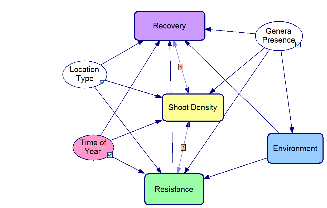
(a) Overall network

(b) Resistance subnetwork

(c) Recovery subnetwork

(d) Shoot density subnetwork

Figure 2: Overall seagrass DBN model (Wu et al., 2018) (Fig. 2a). Nodes are ovals and arrows denote conditional dependence between a parent and child node in the same time-slice. Where an arrow is labelled with a $1$, the child node is in the next time-slice. Rounded rectangles denote subnetworks. Yellow nodes relate to loss and recovery in shoot density, purple nodes to recovery, green nodes to resistance, blue nodes to environmental factors and pink for all other nodes. The environment subnetwork is not shown as it is a disjoint subnetwork of the blue nodes, which are effectively inputs to the model.

For one time-slice of this DBN, DCMAP finds a total of 30 optimal cluster mapping solutions, with an optimal cost of 1371.4 compared to a naive heuristic cost of 34444; the first optimal solution was found at iteration 934 and the last one at iteration 8135. Over 20 runs, the mean iteration for the first optimal solution was 934 $(\text{95\% CI }926,971)$. However, a near-optimal solution that was within 5.0% of the optimal cost was found at iteration 170 with a cost of 1421.2 (Fig. 3).

For the two time-slice version of this DBN with 50 nodes, the in- and out-degrees are even higher than the one time-slice DBN (Table 4).

Table 4: Distribution of in- and out-degree (degree and number of nodes with that degree) two time-slice DBN.

In-degree	0	1	2	3	4	5	6	7	8
#nodes	18	4	10	6	5	2	2	2	1
Out-degree	0	1	2	3	4	6	7	8	9
#nodes	3	27	7	6	2	1	1	1	2

The optimal cost solution has a cost of 6221.4 compared to the naive heuristic cost of 3148386, and there are 30 optimal solutions with the first found at iteration 4342 and the last at iteration 19483. Over 20 runs, the mean iteration for the first optimal solution was 2256 $(2150,2271)$. This time, a near-optimal solution that was within 10.0% of the optimal cost (a cost of 6382.8) was found at iteration 1794; a solution within 20% of the optimal cost (cost of 7431) was found at iteration 885. It takes just 255 iterations to find a cluster mapping that has less than one tenth the cost of the naive heuristic compared to 94 iterations for the one time-slice DBN (Fig. 3). Like our simple example, DCMAP rapidly converged onto near-optimal solutions, and regularly returned cluster mapping solutions (Fig. 3), on average returning a solution every 8.2 and 14.2 iterations for the one and two time-slice versions of the study.

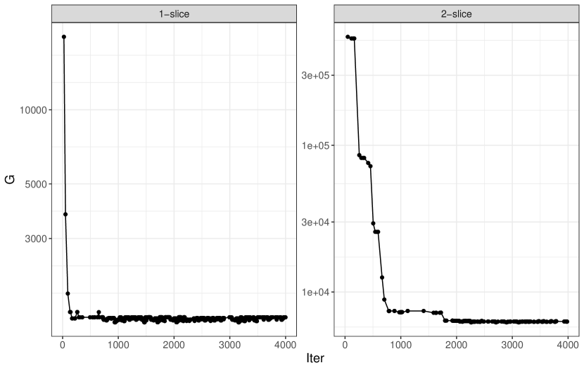
Figure 3: Cost $G$ of solutions found and the iteration of their discovery for both the one and two time-slice DBNs.

Furthermore, we could compare the similarity of cluster mappings to optimal cluster mappings using nodes assigned to the same cluster rather than nodes assigned to the same cluster label, as labels could vary depending on its child clusters when assigning a node to an existing cluster (Section 2.3.1). See Section 6.2 for a discussion about label switching. This could be done by creating a $n\times n$ matrix where $Y[i,j]\in\{0,1\}$ for each cluster mapping, where a 1 indicates that those two nodes are in the same cluster. This way, the similarity of a solution $Y$ compared to an optimal solution $Y^{\ast}$ could be computed as the dot product $Y\boldsymbol{\cdot}Y^{\ast}$, divided by the number of ones in $Y^{\ast}$. Here, we use the maximum similarity between $Y$ and the set of optimal solutions $\boldsymbol{Y}^{\ast}$. For the one time-slice DBN, there was both rapid convergence in terms of cost (Fig. 3) and approximately 80% or more similarity (Fig. 4) to optimal solutions in just a few hundred iterations. The two time-slice DBN needed about 800 to 2000 iterations to converge to near-optimal cost, finding the optimal solution at ieration 2256; the solutions discovered at iterations 885 and 1794 shared 72% and 88% similarity with the optimal solution, respectively.

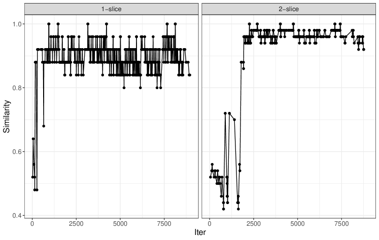
Figure 4: Similarity of solutions to the set of optimal solutions and their iteration of discovery for both the one and two time-slice DBNs.

For context, the size of the search space was $1.51\times 10^{21}$ and $9.91\times 10^{9}$ for the two and one time-slice DBNs, respectively and, as might be expected given Lemma 4.4, all branch solutions are unique (i.e. no two branches with the same solution). In both cases, even the near-optimal solutions were less than 4.4% and 0.2% the cost of the naive solutions, corresponding to a computational speed-up of 22.8 and 426, respectively. Therefore, our approach enables non-homogeneous DBN inference of our case study model in a MCMC framework.

6 Discussion

6.1 Computation Cost and Cluster Mapping Cost

Empirical results suggest that the proposed algorithm is very fast in terms of computation time, especially for finding near-optimal solutions. This can be attributed to the combination of the DAG structure and a search that is constrained along active branches (branches where $\text{Br}_{\text{pl}}(b)>q\$l$ for at least one proposal in the queue, Theorem 4.6) that is guided by a heuristic. Consider, for instance, the first four iterations in the search of the one time-slice DBN case study (Section 5). Note that $iter$ is the iteration number, and columns $12,15,21..25$ show the cluster mapping for those nodes; nodes 24 and 25 are leaf nodes.

$$\footnotesize\setcounter{MaxMatrixCols}{14}\begin{bmatrix}iter&l&k&b&G(b,l)&\hat{g}&\text{G}_{\text{min}}&12&15&21&22&23&24&25\\ 1&0&1&1&50&34456&34444&0&0&0&0&0&0&1\\ 2&0&2&1&143&33631&34444&0&0&0&0&0&2&1\\ 3&1&2&1&172&32783&34444&2&0&0&0&0&2&1\\ 3&1&2&2&247&33547&34444&0&0&0&0&2&2&1\\ 3&1&2&3&507&30235&34444&2&0&0&0&2&2&1\\ 4&2&2&3&630&31429&34444&2&2&0&0&2&2&1\\ 4&2&2&4&607&29198&34444&2&0&0&2&2&2&1\\ 4&2&2&5&1934&28044&34444&2&2&0&2&2&2&1\\ \end{bmatrix}$$

The two leaf nodes are popped in iterations one and two, completing layer 0 and leading to popping of cluster-layer $(k,l)=(2,1)$ in iteration 3 on branch 1. Of the three possible cluster mapping combinations generated on branch 1 in iteration 3, the third proposal has the least heuristic estimated total cost $\hat{g}$, and is chosen to be popped in iteration 4. The constraint of branch activation is that only cluster mapping proposals that reside on one branch can be used for each layer, but switching to lower cost branches is possible between layers. It can be seen that with just four iterations, there is already an 18.5% reduction in projected total cost; this is an upper bound of the true cost for the heuristic used in this case study. Such a rapid reduction in total cluster mapping cost $G$ arises in part because of layer-by-layer best-first optimisation using transition costs $c$ (18) and because cluster mapping can significantly affect propagation of probabilities between layers and thus the cost. Ultimately, our adaptive constraint and release of branches along with heuristic search facilitates fast discovery of near-optimal solutions.

The worst case computational scenario for many heuristic search algorithms like A*, which are also referred to as best first search, are local minima that arise as a result of both the nature of the search space and the heuristic function (LaValle, 2006). In these scenarios, best first search algorithms overcome the local minima by searching all possible states within the minima, before escaping. DCMAP provides an innate strategy to help overcome local minima due to a combination of branch constraint and random activation. In the former, constraining the number of active branches (line 22 of Algorithm 3) to only one at the completion of each layer helps to minimise the number of iterations wasted searching a local minima by constraining the size of $Q^{\prime}$. For the latter, random switching between best first and breadth first search allows the algorithm to explore other parts of the DAG cluster mapping search space to help overcome local minima. Our approach is like a hybrid of graph growing (breadth-first) partitioning and iterative improvement heuristic partitioning (search prioritised search) (Buluç et al., 2016).

In our two time-slice DBN case study, cluster mapping solutions found between iterations 800 and 1700 have low costs (Fig. 3) and about 70% similarity with the optimal mapping (Fig. 4), suggesting the presence of local minima. However, the switching between best first and breadth first search enables relatively rapid convergence to solutions with high similarity with optimal solutions and near-optimal cost, and discovery of optimal solutions in $O(n^{2})$ time ($n$ is the number of nodes). Determined empirically, this is efficient given the exponential in $n$ search space size (Section 2.4). As is typical for best first search, a more informed heuristic enables more rapid algorithm convergence (LaValle, 2006). This appears to be the case for our one time-slice DBN case study, which converges to near-optimal cost and 72% similarity with the optimal solution in just 178 iterations, and tends to stay above 80% similarity thereafter.

Although our algorithm is efficient, finding all optimal solutions is computationally expensive. Our empirical study suggests that, as supported theoretically since dominated solutions are always pruned (Section 4 and Corollary 4.1), $G$ trends downwards over search iterations (Fig. 3) and, in the case of $\text{G}_{\text{min}}$, is monotonic in its change over iterations (Fig. 5). As a result, if the application only requires one solution, then the search could be terminated early if $\text{G}_{\text{min}}$ does not change over a specified number of iterations; in our case study, a maximum of 566 and 615 iterations between successive drops in $\text{G}_{\text{min}}$ were observed. Future research could study convergence characteristics of the algorithm and provide guidelines for termination.

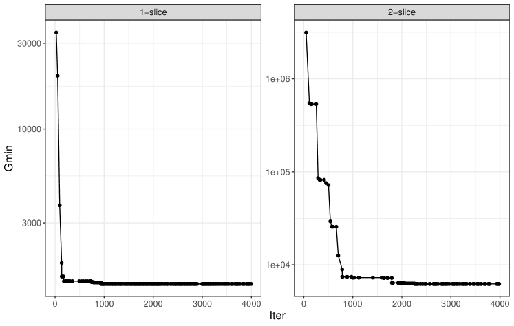
Figure 5: $\text{G}_{\text{min}}$ plotted over iterations, starting from iteration 182 and 169 for one and two time-slice DBNs, respectively, for visual clarity since the cost of earlier iterations are exponentially higher.

Traditionally, dynamic programming based approaches require PSPACE memory due to a need to store proposed actions at each stage (equation 13) (LaValle, 2006). Although sparse matrices help with reducing memory requirement, as does branch pruning, this is still an area for future research for DCMAP. One potential approach to reduce memory complexity is to sample proposals rather than generating all possible combinations of proposals. Additionally, alternative approaches to algorithm termination could be investigated, such as when the change in total cost of successive cluster mapping solutions is relatively small. Echoing the findings of Buluç et al. (2016), a better understanding of how heuristics and branch constraint and activation contributes to search efficiency could also help inform algorithm termination and early termination for near-optimal solutions.

6.2 Contextualisation in Literature and Application

Our case study showed that DCMAP was highly effective at rapidly finding near-optimal cluster mappings, ranging from $O(n)$ to $O(n^{2})$ iterations depending on the threshold applied. In addition, some of these near-optimal solutions demonstrated high similarity to optimal cluster mapping solutions, but more diverse solutions could exist due to local minima with similar cost to the optimal cost. The first optimal solution tended to be found in $O(n^{2})$ iterations. In our case study, cluster-based DBN inference had the potential for up to 426 times speed-up of computation compared to baseline variable elimination, enabling MCMC inference of a complex systems DBN to support ecosystem managers with better modelling of uncertainty.

Although our empirical case study was for a discrete BN, the proposed algorithm equally applies to discrete or continuous or hybrid BNs, DBNs and Markov models in general, or indeed to hierarchical or multilevel models with Bayesian inference (Gelman et al., 2013); the key adaptation required is the development of an application-specific cost function. The proposed method can be directly applied to templated BNs such as DBNs or Object Oriented Bayesian Networks (OOBNs) (Koller and Pfeffer, 2013). The dynamic model can be unrolled (Wu et al., 2018) into a BN and cluster mapping performed on the result. In practice, for a $k^{th}$ order dynamic model, running cluster mapping on $k$ slices is sufficient to find optimal clusters that can then be replicated over all slices.

The key assumption here is that the cost of a cluster can have dependence based on the mapping of connected clusters, and it is non-negative and non-zero. For statistical inference contexts, cost dependency can result in markedly different local costs given the cluster mappings of connected nodes, and thus impact the global optimality of the cluster mapping solution (Section 1.1). However, despite the plethora of methods in graph partitioning (Buluç et al., 2016; Bader et al., 2013), including those based on dynamic programming (Zheng et al., 2020) or even layer-based approaches (van Bevern et al., 2017), cost dependency is not explicitly modelled. Hence it is not possible to benchmark our work against theirs degree given the added complexity of cost dependency. On the other hand, although cluster-like structures have been used widely in statistical inference for DAGs, such as based on BE (Dechter, 1999) and clustering (Lauritzen and Spiegelhalter, 1988; Daly et al., 2011; Shiguihara et al., 2021), none of the reviewed literature explicitly optimised clusters for inference, and cluster-like structures were mostly focused on improving computational efficiency. For instance, as noted in Section 1.1, Lauritzen and Spiegelhalter (1988) used a heuristic (triangulation) to reduce computation cost, and Gu and Zhou (2020) a heuristic to partition a BN for learning. However, heuristics are typically context specific and optimisation is needed to better understand how heuristics perform in new contexts (i.e. new cost functions).

This paper developed a novel, optimal cluster mapping algorithm, DCMAP, which can be used to facilitate inference. A natural direction for future work includes the study of inference using optimal cluster mappings, building on the adaptation of Wu et al. (2018) here (Section 1.1). This could include guidelines for cost function design, memory-computation time trade-offs, and embedding BN inference in a MCMC framework like Shafiee Kamalabad and Grzegorczyk (2020). The ability for DCMAP to optimise for arbitrary dependent costs opens up new research opportunities in: (i) reducing DAG model computation time through clustering, (ii) inferring model parameters, such as homogeneous clusters of a non-homogeneous system, and (iii) hybrid approaches for inference combining optimisation (DCMAP) and Bayesian statistical inference, like the combination of gradient optimisation and variational inference (Mohamad et al., 2020) or partitioning and estimation for learning BN structures (Gu and Zhou, 2020). Building on the work of Gu and Zhou (2020), optimal partitioning with arbitrary cost functions using DCMAP could open up new research directions in BN and DBN research. The latter two applications of DCMAP could explore different information measures such as AIC and WAIC, in-sample and out-of-sample error (such as that used in machine learning), as well as computational cost. For instance, DCMAP could potentially be used to support inference in non-homogeneous Hidden Markov Models or DBNs to find optimal cluster mappings that describe homogeneous portions of a non-homogeneous system, akin to changepoint detection and model switching, or system state (Shafiee Kamalabad and Grzegorczyk, 2020; Boys et al., 2000). Based on these mappings, model parameters could then be updated as part of MCMC. Boys et al. (2000) found that performing full forward-backward inference of state at each MCMC step for a homogeneous HMM helped to expedite model convergence; potentially, an integrated optimisation step (DCMAP) might help accelerate convergence in a non-homogeneous system.

Finally, an additional advantage of our method is that the proposal of cluster mappings (Section 2.3.1) produces unique mapping solutions in each branch (Lemma 4.4). Hence, there is an innate potential for parallel computation for future study. Additionally, although there is still the potential for label switching where the same partitions are found but with different cluster labels, this is not an issue that affects algorithm convergence to the same extent as in MCMC. However, the properties of resultant clusters and strategies to avoid label switching warrant future investigation.

7 Supplementary Material: Inference Example

7.1 Lauritzen and Spiegelhalter (1988) Clustering Calculations

Initialise $AF$: 2+4
Initialise $ABD$: 8
Initialise $CE$: 2+4
Initialise $DEG$: 8
Project and absorb $AF$ to $ABD$: $2\times 0.6+2\times 3+8$
Project and absorb $CE$ to $DEG$: $2\times 0.6+2\times 3+8$
Project and absorb $ABD$ to $DEG$: $(4+2)\times 0.6+2\times 3+8$
Project and absorb $DEG$ to $ABD$: $(4+2)\times 0.6+2\times 3+8$
Project and absorb $ABD$ to $AF$: $(4+2)\times 0.6+2\times 3+4$
Project and absorb $DEG$ to $CE$: $(4+2)\times 0.6+2\times 3+4$
Marginalisation costs for each of $A,F,C,E$: 1.2 Marginalisation costs for each of $B,D,G$: 2.4 Total: 132.8

7.2 DCMAP Clustering Calculations

$$P^{f}_{\boldsymbol{X}_{10}}(A,F)=P(A)P(F|A), \text{ cost }8$$ (26)

$$P^{f}_{\boldsymbol{X}_{12}}(A)=\sum\limits_{F}{P^{f}_{\boldsymbol{X}_{10}}(A,F)}, \text{ cost }1.2$$ (27)

$$P^{f\prime}_{\boldsymbol{X}_{10}}(A,F)=P^{f}_{\boldsymbol{X}_{10}}(A,F)\sum\limits_{B}{P^{b}_{\boldsymbol{X}_{21}}(A,B)}, \text{ cost }7.2$$ (28)

$$P^{f}_{\boldsymbol{X}_{62}}(B)=P(B), \text{ cost }2$$ (29)

$$P^{f}_{\boldsymbol{X}_{72}}(C)=P(C), \text{ cost }2$$ (30)

$$P^{f}_{\boldsymbol{X}_{21}}(D)=\sum\limits_{A,B}{P(D|A,B)P^{f}_{\boldsymbol{X}_{12}}(A)P^{f}_{\boldsymbol{X}_{62}}(B)}, \text{ cost }17.6$$ (31)

$$P^{f}_{\boldsymbol{X}_{31}}(E)=\sum\limits_{C}{P(E|C)P^{f}_{\boldsymbol{X}_{72}}(C)}, \text{ cost }7.2$$ (32)

$$P^{f}_{\boldsymbol{X}_{20}}(G)=\sum\limits_{E}{P(G|D,E)P^{f}_{\boldsymbol{X}_{21}}(E)P^{f}_{\boldsymbol{X}_{21}}(D)}, \text{ cost }17.6$$ (33)

$$P^{b}_{\boldsymbol{X}_{20}}(D,E)=\sum\limits_{G}{P(G|D,E)}, \text{ cost }10.4$$ (34)

$$P^{b}_{\boldsymbol{X}_{21}}(A,B)=\sum\limits_{D}{P(D|A,B)}\sum\limits_{E}{P_{\boldsymbol{X}_{20}}(D,E)}, \text{ cost }13.6$$ (35)

$$P^{b}_{\boldsymbol{X}_{31}}(E,C)=P(E|C)\sum\limits_{D}{P^{b}_{\boldsymbol{X}_{20}}(D,E)}, \text{ cost }7.2$$ (36)

$$P^{b}_{\boldsymbol{X}_{62}}(B)=P(B)\sum\limits_{A}{P^{b}_{\boldsymbol{X}_{21}}(A,B)}, \text{ cost }5.2$$ (37)

$$P^{b}_{\boldsymbol{X}_{72}}(C)=P(C)\sum\limits_{E}{P^{b}_{\boldsymbol{X}_{31}}(E,C)}, \text{ cost }5.2$$ (38)

Consider the calculation of cost for $P^{f}_{\boldsymbol{X}_{21}}(D)$ above, which comprises propagation of partial results from parent clusters and then multiplication and marginalisation by cluster-layer $\boldsymbol{X}_{21}$, hence a cost of $2+4+8+(4+2)\times 0.6=17.6$.

In cluster 1 (nodes $A$ and $F$), $P^{f}_{\boldsymbol{X}_{12}}(A)$ is used to propgate partial results outwards to child clusters, whereas $P^{f\prime}_{\boldsymbol{X}_{10}}(A,F)$ propgates child cluster partial results into cluster 1. $P(A)$ and $P(F)$ can be obtained from the latter at a cost of 1.2 each.

$P(G)$ comes directly from $P^{f}_{\boldsymbol{X}_{20}}(G)$. Similarly, $P(B)$ and $P(C)$ come from $P^{b}_{\boldsymbol{X}_{72}}(B)$ and $P^{b}_{\boldsymbol{X}_{72}}(C)$, respectively.

$P(D)$ is obtained by combining partial results $P(D)=P^{f}_{\boldsymbol{X}_{21}}(D)\sum\limits_{E}{P^{b}_{\boldsymbol{X}_{20}}(D,E)}$ at a cost of 5.2.

$P(E)$ is obtained by combining partial results $P(E)=P^{f}_{\boldsymbol{X}_{31}}(E)\sum\limits_{D}{P^{b}_{\boldsymbol{X}_{20}}(D,E)}$ at a cost of 5.2.

Total cost is 117.2

8 Supplementary Material: Illustrative Example

We demonstrate the steps of the algorithm using the illustrative example described in Section 3.1. We have $n=7$ nodes labelled $A$ through $G$ and indexed from $i=1$ to $7$, respectively. There are three layers so the last layer is $L=2$. For the purposes of new cluster proposals, we associate $F$ and $G$ in layer 2 with clusters 1 and 2, $D$ and $E$ in layer 1 with cluster 3 and 4, and $A$, $B$, $C$ with clusters 5, 6 and 7, respectively. For this example, $F$ and $G$ are assigned to clusters 1 and 2, respectively, so $\hat{\textrm{U}}[1,1,6]=1$ and $\hat{\textrm{U}}[1,2,7]=1$, and ${\textrm{G}}[1,1..7]=h(\boldsymbol{X})=85.8=\text{G}_{\text{min}}$, which is the computational cost for evaluating:

$$\sum\limits_{C}{P(C)}\sum\limits_{B}{P(B)}\sum\limits_{A}{P(A)}\sum\limits_{D}{P(D|A,B)}\sum\limits_{E}{P(E|C)}$$

$$\sum\limits_{G}{P(G|D,E)}\sum\limits_{F}{P(F|A)}.$$ (39)

Thus, two entries, both eligible for popping by definition of a leaf node, are added to the queue $Q=Q^{\prime}=\begin{bmatrix}b=1&u(\boldsymbol{X}_{kl})=1&l=0&\hat{g}(\boldsymbol{X}_{kl})=85.8\\ b=1&u(\boldsymbol{X}_{kl})=2&l=0&\hat{g}(\boldsymbol{X}_{kl})=85.8\end{bmatrix}$.

At the first iteration, cluster-layer $(k=1,l=0)$ on branch $b=1$ is popped from the queue $Q$ (noting that ties in $\hat{g}$ are broken arbitrarily). Only one node $F$ (index $i=6$), has been proposed to be in this cluster-layer as $\hat{\textrm{U}}[b=1,k=1,i=1..7]=\{0,0,0,0,0,1,0\}$, thus $N=1$ and $\boldsymbol{X}_{1}=\{F\}$ when generating combinations at line 14. Using (18), the objective function cost is:

$$\text{G}[b=1,l=0]=0+c\Bigl{(}J\bigl{[}F,1,\varnothing,\varnothing\bigr{]}\Bigr{)}=5.2$$

since there are no previous layers. As all nodes are assumed to have 2 states and there are no child nodes to multiply by in $J$, the multiplication cost is just that for the $2\times 2$ CPT matrix $P(F|A)$, which is $4$. As we are propagating backward, layer-by-layer through the DAG, we need to marginalise $F$ and we assume the cost of each summation operation to be 0.6. The result is a $2\times 1$ matrix $\pi(A)$ with probabilities corresponding to states $a_{1}$ and $a_{2}$. Adding this cost to a simple backward elimination for the heuristic, we arrive at an estimate:

$$\hat{g}(\boldsymbol{X}_{kl}) =c\Bigl{(}J\bigl{[}\boldsymbol{X}_{kl},u(\boldsymbol{X}_{kl}),J(\boldsymbol{X}_{k,l^{\prime}<l}),J(\boldsymbol{X}_{k^{\prime}\neq k,l^{\prime}<l})\bigr{]}\Bigr{)}+$$

$$h\Bigl{(}\boldsymbol{X}\setminus\bigl{(}\boldsymbol{X}_{kl|k\in M_{l}}\cup\boldsymbol{X}_{0..l-1}\bigr{)}\Bigr{)}$$

$$=c\Bigl{(}J\bigl{[}F,1,\varnothing,\varnothing\bigr{]}\Bigr{)}+h\Bigl{(}\{A,B,C,D,E,G\}\Bigr{)}$$

$$=5.2+82.6=87.8$$ (40)

where $h\Bigl{(}\{A,B,C,D,E,G\}\Bigr{)}$ is the cost to evaluate:

$$\sum\limits_{C}{P(C)}\sum\limits_{B}{P(B)}\sum\limits_{A}{P(A)}\sum\limits_{D}{P(D|A,B)}\sum\limits_{E}{P(E|C)}$$

$$\sum\limits_{G}{P(G|D,E)\mathcal{P}(A)}.$$

As not all layer $l=0$ nodes have been assigned to a cluster yet, we skip layer updates (line 21) and go directly to proposing clusters for parent nodes (line 25). Only node $A$ is a parent of $F$, which could be assigned to the same cluster as $F$ (cluster 1) or to its own unique cluster (cluster 5), which results in updates to $\hat{\textrm{U}}$ for branch 1 and addition of entries $\boldsymbol{q}$ to $Q$ as follows:

$$\hat{\textrm{U}}[1,1..7,1..7]=\begin{bmatrix}1&0&0&0&0&1&0\\ 0&0&0&0&0&0&1\\ 0&0&0&0&0&0&0\\ 0&0&0&0&0&0&0\\ 1&0&0&0&0&0&0\\ 0&0&0&0&0&0&0\\ 0&0&0&0&0&0&0\\ \end{bmatrix}$$

$$\boldsymbol{q}=\begin{bmatrix}b&u(\boldsymbol{X}_{kl})&l&\frac{1}{\hat{g}(\boldsymbol{X}_{kl})}&G\\ 1.000&1.000&2.000&0.011&5.200\\ 1.000&5.000&2.000&0.011&5.200\\ \end{bmatrix}$$

Note that as $Q$ is a sparse matrix, we can equivalently pop least cost proposals by inverting $\hat{g}(\boldsymbol{X}_{kl})$ and finding the maximum.

Consider iteration 4 of the algorithm, at a point where cluster mappings on branch 1 are $\text{U}[1,\{D,F,G\}]=\{1,1,2\}$ and cluster $k=2$ has been proposed for nodes D and E. Cluster-layer $(k=2,l=1)$ is being updated on branch 1. However, as node D has already been updated on this branch, only E or the empty set (proposed for branch 3) can be considered as proposals based on this branch (line 14). Note that the empty set branch preserves existing mappings in this layer and enables future updating with cluster proposals for node E other then $k=2$. The updated cost values for branch 1 are $G(l=1)=35.2$ and $\hat{g}(\boldsymbol{X}_{kl})=75.8$ which is an improvement on the original estimate of total cost in iteration 1. This time, a layer has been completed which means that branch 1 is ready for updates at layer 2, hence $\text{Br}_{\text{pl}}(1)=l+1=2$. In addition, if there were other branches $i$ with the same cluster mapping in layer 1 where $\text{U}[i,\{D,E\}]=\{1,2\}$, then a link would be made between branches $b^{\prime}$ and $i$ in $\text{Br}_{\text{lk}}$ (line 24). This means that, should one of these branches be popped in the future, any linked, dominated branches would be pruned (line 12).

At the end of this iteration, the cluster mapping proposals for branch 1 are updated and now include a number of mappings for nodes $A$, $B$ and $C$ compared to iteration 1. In addition, four more entries $\boldsymbol{q}$ are added to the queue $Q$, the first two due to creation of a new branch (line 16), and the latter two from proposal of cluster-layers for parent nodes $E$ and $C$ as the same or a new cluster (line 25).

$$\hat{\textrm{U}}[1,1..7,1..7]=\begin{bmatrix}1&1&0&1&0&1&0\\ 0&0&1&1&1&0&1\\ 0&0&0&0&1&0&0\\ 0&0&0&1&0&0&0\\ 1&0&0&0&0&0&0\\ 0&1&0&0&0&0&0\\ 0&0&1&0&0&0&0\\ \end{bmatrix}$$

$$\boldsymbol{q}=\begin{bmatrix}b&u(\boldsymbol{X}_{kl})&l&\frac{1}{\hat{g}(\boldsymbol{X}_{kl})}&G\\ 3.000&4.000&1.000&0.012&15.600\\ 3.000&3.000&1.000&0.012&15.600\\ 1.000&2.000&2.000&0.013&35.200\\ 1.000&7.000&2.000&0.013&35.200\\ \end{bmatrix}$$

References

- Ahn et al. (2018) Ahn, S., M. Chertkov, J. Shin, and A. Weller (2018). Gauged mini-bucket elimination for approximate inference. In International Conference on Artificial Intelligence and Statistics, pp. 10–19. PMLR.
- Bader et al. (2013) Bader, D. A., H. Meyerhenke, P. Sanders, and D. Wagner (2013). Graph Partitioning and Graph Clustering, Volume 588. Providence, Rhode Island: AMS.
- Belfodil et al. (2019) Belfodil, A., A. Belfodil, and M. Kaytoue (2019). Anytime subgroup discovery in numerical domains with guarantees. In Joint European Conference on Machine Learning and Knowledge Discovery in Databases, pp. 500–516. Springer.
- Bellman and Dreyfus (1962) Bellman, R. E. and S. E. Dreyfus (1962). Applied Dynamic Programming. Princeton University Press.
- Boys et al. (2000) Boys, R. J., D. A. Henderson, and D. J. Wilkinson (2000). Detecting homogeneous segments in dna sequences by using hidden markov models. Journal of the Royal Statistical Society: Series C (Applied Statistics) 49(2), 269–285.
- Buluç et al. (2016) Buluç, A., H. Meyerhenke, I. Safro, P. Sanders, and C. Schulz (2016). Recent Advances in Graph Partitioning, pp. 117–158. Cham: Springer International Publishing.
- Daly et al. (2011) Daly, R., Q. Shen, and S. Aitken (2011). Learning bayesian networks: approaches and issues. The Knowledge Engineering Review 26(02), 99–157.
- Dechter (1999) Dechter, R. (1999). Bucket elimination: A unifying framework for reasoning. Artificial Intelligence 113(1–2), 41–85.
- Fog (2022) Fog, A. (2022). Instruction Tables: : Lists of instruction latencies, throughputs and micro-operation breakdowns for Intel, AMD and VIA CPUs. Technical University of Denmark.
- Gelman et al. (2013) Gelman, A., J. B. Carlin, H. S. Stern, D. B. Dunson, A. Vehtari, and D. B. Rubin (2013). Bayesian Data Analysis (3rd ed.). Boca Raton, Fla.: Chapman and Hall, CRC.
- Gu and Zhou (2020) Gu, J. and Q. Zhou (2020, jan). Learning big gaussian bayesian networks: Partition, estimation and fusion. J. Mach. Learn. Res. 21(1).
- Hart et al. (1968) Hart, P. E., N. J. Nilsson, and B. Raphael (1968). A formal basis for the heuristic determination of minimum cost paths. IEEE Trans. Systems Science and Cybernetics 4(2), 100–107.
- Koller and Pfeffer (2013) Koller, D. and A. Pfeffer (2013). Object-oriented Bayesian networks. arXiv:1302.1554.
- Kschischang et al. (2001) Kschischang, F. R., B. J. Frey, and H.-A. Loeliger (2001). Factor graphs and the sum-product algorithm. Information Theory, IEEE Transactions on 47(2), 498–519.
- Lauritzen and Spiegelhalter (1988) Lauritzen, S. L. and D. J. Spiegelhalter (1988). Local computations with probabilities on graphical structures and their application to expert systems. Journal of the Royal Statistical Society. Series B (Methodological) 50(2), 157–224.
- LaValle (2006) LaValle, S. M. (2006). Planning Algorithms. Cambridge University Press.
- Levin and Lubchenco (2008) Levin, S. A. and J. Lubchenco (2008). Resilience, robustness, and marine ecosystem-based management. BioScience 58(1), 27–32.
- Likhachev et al. (2005) Likhachev, M., D. I. Ferguson, G. J. Gordon, A. Stentz, and S. Thrun (2005). Anytime dynamic A*: An anytime, replanning algorithm. In ICAPS, Volume 5, pp. 262–271.
- Mohamad et al. (2020) Mohamad, S., A. Bouchachia, and M. Sayed-Mouchaweh (2020). Asynchronous stochastic variational inference. In L. Oneto, N. Navarin, A. Sperduti, and D. Anguita (Eds.), Recent Advances in Big Data and Deep Learning, Cham, pp. 296–308. Springer International Publishing.
- Murphy (2002) Murphy, K. P. (2002). Dynamic Bayesian networks: representation, inference and learning. Ph. D. thesis, University of California, Berkeley.
- Park and Darwiche (2004) Park, J. D. and A. Darwiche (2004). Complexity results and approximation strategies for map explanations. Journal of Artificial Intelligence Research 21, 101–133.
- Shafiee Kamalabad and Grzegorczyk (2020) Shafiee Kamalabad, M. and M. Grzegorczyk (2020). Non-homogeneous dynamic bayesian networks with edge-wise sequentially coupled parameters. Bioinformatics 36(4), 1198–1207.
- Shiguihara et al. (2021) Shiguihara, P., A. D. A. Lopes, and D. Mauricio (2021). Dynamic Bayesian network modeling, learning, and inference: A survey. IEEE Access 9, 117639–117648.
- van Bevern et al. (2017) van Bevern, R., R. Bredereck, M. Chopin, S. Hartung, F. Hüffner, A. Nichterlein, and O. Suchỳ (2017). Fixed-parameter algorithms for dag partitioning. Discrete Applied Mathematics 220, 134–160.
- Watts and Strogatz (1998) Watts, D. J. and S. H. Strogatz (1998). Collective dynamics of small-world networks. Nature 393(6684), 440–442.
- Wu et al. (2018) Wu, P. P.-Y., M. J. Caley, G. A. Kendrick, K. McMahon, and K. Mengersen (2018). Dynamic Bayesian network inferencing for non-homogeneous complex systems. Journal of the Royal Statistical Society, Series C 67(2), 417–434.
- Zheng et al. (2020) Zheng, S., X. Zhang, D. Ou, S. Tang, L. Liu, S. Wei, and S. Yin (2020). Efficient scheduling of irregular network structures on cnn accelerators. IEEE Transactions on Computer-Aided Design of Integrated Circuits and Systems 39(11), 3408–3419.