The Widths of Strict Outerconfluent Graphs

Abstract

Strict outerconfluent drawing is a style of graph drawing in which vertices are drawn on the boundary of a disk, adjacencies are indicated by the existence of smooth curves through a system of tracks within the disk, and no two adjacent vertices are connected by more than one of these smooth tracks. We investigate graph width parameters on the graphs that have drawings in this style. We prove that the clique-width of these graphs is unbounded, but their twin-width is bounded.

1 Introduction

Confluent drawing is a powerful style of graph drawing that permits many non-planar and dense graphs to be drawn without crossings [9, 10, 16, 17, 11, 19, 8]. A confluent drawing consists of a system of non-crossing smooth curves in the plane, called tracks, whose endpoints are either vertices of the graph or junctions where several tracks meet, all having the same slope at that point. Two vertices are adjacent whenever the union of some of the tracks forms a smooth curve connecting them. In this way, each confluent drawing represents unambiguously a unique graph, unlike the bundled drawings which they otherwise resemble. Applications of confluent drawing include the automated layout of syntax diagrams [1], and the simplification of the Hasse diagrams of partially ordered sets [13]. A constrained version of confluent drawing, called strict confluent drawing, requires that each adjacency be represented by only one smooth curve [12, 14]. In outerconfluent drawings, the tracks are interior to a disk whose boundary contains the vertices. In this work we study strict outerconfluent graphs, the graphs that have strict outerconfluent drawings. If the vertex ordering along the drawing boundary is given, these graphs may be recognized in polynomial time [12], but their recognition without this information, and other algorithmic problems concerning them, remain mysterious.

In this work, following Förster et al. [14], we study the width of strict outerconfluent graphs. There are many graph width parameters, of which treewidth is perhaps the most famous. Treewidth is bounded for some types of graph drawing with vertices on the boundary of a disk (outerplanar and outer-$k$-planar drawings [21]), suggesting that, analogously, strict outerconfluent graphs might have bounded width of some sort. However, graphs of bounded treewidth are sparse, and strict outerconfluent graphs can be dense: for instance they include the complete graphs and complete bipartite graphs. Therefore, a different concept of width is needed, one that can be bounded for dense graphs. Among these widths, we focus on two, clique-width and twin-width.

For sparse graphs, clique-width is equivalent to treewidth, in the sense that if one of these two width parameters is bounded, the other one is also bounded [15], but graphs of bounded clique-width can also be dense. The strict outerconfluent graphs include the distance-hereditary graphs, which are known to have bounded clique-width [10]. Förster et al. [14] defined a sub-class of strict outerconfluent drawings, the tree-like outerconfluent drawings, in which the tracks that are incident to junctions must form a single topological tree within the drawing, and proved that their graphs also have bounded clique-width [14]. We prove that, in contrast, there exist strict outerconfluent graphs with unbounded clique-width.

To complement this result, we prove that another width parameter of these graphs, their twin-width, is bounded. Twin-width is bounded for many classes of graphs of interest in graph drawing, including the planar and $k$-planar graphs, and the graphs of bounded genus. It is also bounded for graphs of bounded clique-width [3]. The algorithmic consequences of bounded twin-width include the existence of a fixed-parameter tractable algorithm for testing whether a given graph models a given formula of first-order logic, parameterized by the size of the formula (including as a special case subgraph isomorphism) [7], and better approximation algorithms for dominating set, independent set, and graph coloring than the best approximations known for more general families [4, 2].

We prove the following results:

• The strict outerconfluent graphs do not have bounded clique-width (Theorem 1).

• The strict outerconfluent graphs have bounded twin-width. A twin-width decomposition of bounded width can be constructed for these graphs in polynomial time, given their vertex ordering around the boundary of a strict outerconfluent drawing.

The main idea of the first result is to find a recursive construction of a family of strict outerconfluent drawings for which we can prove unbounded rank-width, a graph width parameter closely related to clique-width. The main idea of the second result is to harness known results relating the growth rate of a family of ordered graphs (pairs of a graph and a linear ordering on its vertices) to the twin-width of the family, and to use the fact that strict confluent drawings have only linearly many junctions [12] to show that they have a small growth rate.

2 Definitions

For completeness we repeat the following definitions, from previous work, of the main concepts considered in our results. We assume familiarity with the basic concepts of graph theory and of two-dimensional topology. By a graph we always mean a finite undirected graph, without multiple adjacencies or loops.

Definition 1.

A strict outerconfluent drawing of a graph $G$ consists of a system of finitely many smooth curves in a topological disk, which we call tracks, disjoint except for shared endpoints. These endpoints have two types: some are identified one-for-one with vertices of $G$, while others are called junctions. Each vertex must lie on the boundary of the disk. At a junction, three or more tracks must meet, all having the same slope. A smooth curve within the union of tracks, starting and ending at vertices and otherwise passing only through tracks and junctions, is called an edge curve. Each two adjacent vertices of $G$ must be the endpoints of a unique edge curve. No edge curve may connect a vertex to itself, or connect non-adjacent vertices. Each track must be part of at least one edge curve. A strict outerconfluent graph is a graph that has a strict outerconfluent drawing.

Definition 2.

The clique-width of an undirected graph is the minimum number of colors needed to construct the graph by a sequence of the following four operations on (improperly) colored graphs:

• Create a single-vertex graph, with its vertex given any of the available colors.

• Take the disjoint union of two colored graphs.

• Recolor all vertices of one color to another color (possibly one that is already used by other vertices).

• Perform a color join operation that adds edges between all pairs of vertices of two specified colors.

Definition 3.

Twin-width is defined through a type of graph decomposition in which clusters of vertices are merged in pairs, starting with one cluster per vertex, until only one cluster is left. At each step of the decomposition, two clusters are connected by a red edge if some but not all adjacencies exist between vertices of one cluster and vertices of the other. The goal is to find a decomposition sequence that minimizes the maximum degree of the resulting sequence of red graphs. The twin-width of a graph $G$ is the minimum value of $d$ such that there exists a decomposition of $G$ for which, after each pairwise merge, the red graph has maximum degree at most $d$ [7].

3 Unbounded clique-width

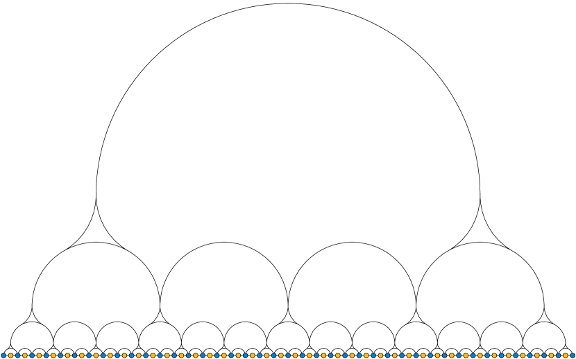
Figure 1: Recursively constructed non-tree-like strict outerconfluent graph $G_{4}$

In this section we prove that strict outerconfluent graphs can have unbounded clique-width. Our proof is based on a family of drawings depicted in Fig. 1, which we construct as follows:

Definition 4.

Let $G_{k}$ be the graph represented by a confluent drawing constructed as follows.

• It is convenient to shape the disk on which the graph is drawn as a half-plane above a horizontal bounding line, to match the depiction in the figure. (This is merely a convention for describing the drawing and does not affect its combinatorial structure.)

• On the boundary line of the half-plane, place $3^{k}$ vertices (the alternating blue and yellow vertices of the figure), connected by tracks that directly connect consecutive pairs of vertices (drawn along the boundary line). These are the only tracks incident to the $\lfloor 3^{k}/2\rfloor$ yellow vertices. Additional tracks will extend vertically from the $\lceil 3^{k}/2\rceil$ blue vertices.

• The remaining tracks of the drawing are arranged into $k$ levels, each of which is drawn within a slab of the half-plane bounded between two horizontal lines. Number these levels from $0$ to $k-1$, bottom to top. The bottom line of the $i$th level contains $\lceil 3^{k-i}/2\rceil$ points (vertices on level $0$, junctions at higher levels) at which tracks extend with a vertical tangent into that level; number these points as $p_{i,j}$ with $0\leq j<3^{k-i}/2$.

• Within level $i$, connect each two consecutive points $p_{i,j}$ and $p_{i,j+1}$ by a semicircle. If $j$ is a multiple of three, subdivide this semicircle by two junctions into three circular arc tracks; for other values of $j$, this semicircle is itself a track. As a special case, for the top level (level $k-1$) the single semicircle connecting points $p_{i,0}$ and $p_{i,1}$ is not subdivided, and forms a track. In the figure, the arcs into which the semicircles are subdivided span angles of $\pi/3$.

• For each level $i$ except the top level, and each subdivided semicircle connecting points $p_{i,j}$ and $p_{i,j+1}$ where $j$ is a multiple of three, add tracks connecting the two subdivision points to the point $p_{i+1,j/3}$ on the upper boundary line of the level. At the two junctions on the semicircle, these tracks should be oriented so that each one connects $p_{i+1,j/3}$ downward by a smooth curve through the semicircle to the two points $p_{i,j}$ and $p_{i,j+1}$. In the figure, these upward tracks are also arcs of circles, congruent to the arcs of the subdivided semicircle.

For instance, the figure depicts $G_{4}$. By construction, $G_{k}$ has exactly $n=3^{k}$ vertices.

Observation 5.

Any semicircular track at level $i$ of $G_{k}$ has smooth paths connecting it to $2^{i}$ vertices, $2^{i-1}$ on its left and $2^{i-1}$ on its right. The track is used by edges of $G_{k}$ that connect each of the vertices in the left subset to each of the vertices in the right subset. These two subsets are separated by a gap of $3^{i-1}$ vertices, wide enough that it cannot be spanned by any semicircular track at a lower level of $G_{k}$.

It follows that $G_{k}$ has $\Theta(4^{k})$ edges, enough to make it not sparse. More precisely, the number of edges can be calculated as

$$\frac{8\cdot 4^{k}-3\cdot 3^{k}-5}{6}.$$

We omit the details as this calculation is not important for our results.

Lemma 6.

$G_{k}$ is strict outerconfluent.

Proof.

Each smooth curve from vertex to vertex must go upward through the levels of the track, follow a single semicircular track at some level, and then go back downwards through the levels, because there are no tracks that smoothly connect downward-going curves to upward-going curves. A smooth curve from vertex to vertex that uses a semicircular track at level $i$ must connect two vertices that are at least $3^{i-1}+1$ steps apart and at most $3^{i}-1$ steps apart. Because these numbers of steps form disjoint ranges for disjoint levels, no two curves using semicircles from different levels can connect the same two vertices. Two semicircular tracks at the same level that do not share a confluent junction have disjoint subsets of vertices that they can reach. Two semicircular tracks at the same level that do share a confluent junction cannot provide two paths between any pair of vertices, because one of the tracks connects vertices that can reach the shared junction to other vertices to the left of the junction, while the other track connects only to the right. ∎

Rather than working directly with clique-width, it is convenient to use rank-width, a closely related quantity derived from hierarchical clusterings of the vertices of a given graph.

Definition 7.

Define a hierarchical clustering of a graph to be a ternary tree having the graph’s vertices as its leaves. For each edge $e$ of such a tree, removing $e$ from the tree partitions it into two subtrees, and thus defines a partition of the vertices into two subsets; call this partition the cut associated with $e$, and call the two subsets the sides of the cut. For any of these cuts, we can form a binary biadjacency matrix whose rows correspond to the vertices on one side of the cut, and whose columns correspond to the vertices on the other side (choosing arbitrarily which side to use for which role). The coefficient of this matrix in a given row and column is one if the corresponding two vertices are adjacent, and zero otherwise. (For the purposes of defining rank-width, these coefficients are defined within the finite field $\mathbb{Z}_{2}$, rather than as real numbers, but that makes little difference for our purposes.) The rank-width of the graph is the maximum rank of any of the biadjacency matrices of these cuts, for a hierarchical clustering chosen to minimize this maximum rank.

Lemma 8 (Oum and Seymour [18]).

Let $G$ be any graph, let $r$ be its rank-width and let $c$ be its clique-width. Then

$$r\leq c\leq 2^{r+1}-1.$$

Thus, the rank-width of a family of graphs is bounded if and only if the clique-width is bounded.

Definition 9.

A balanced cut of an $n$-vertex graph is a partition of its vertices into two subsets that each have at least $n/3$ vertices.

Lemma 10.

Any graph of rank-width $r$ has a balanced cut whose biadjacency matrix has rank $\leq r$.

Proof.

Let $G$ be the given graph, and let $n$ be its number of vertices. Let $T$ be a ternary tree with the vertices of $G$ as its leaves, and with cuts whose biadjacency matrices have rank $\leq r$, which exists by the definition of rank-width. As in Definition 7, define the two sides of an edge $e$ of $T$ to be the two subsets of vertices of $G$ separated in $T$ by $e$. Define a side to be small if it consists of fewer than $n/3$ vertices of $G$, and large otherwise. If we can find an edge with no small side, it will define a balanced cut, which by construction will have rank $\leq r$.

To find an edge of $T$ with no small side, start at any edge of $T$, and then construct a walk as follows. As long as the walk has reached an edge $e$ with a small side, consider the two edges of $T$ that are incident to $e$ on its large side. The large side of $e$ includes $>2n/3$ vertices of $G$ (because the other side is small), so at least one of these two edges, $e^{\prime}$, separates $e$ from $>n/3$ vertices of $G$. Select $e^{\prime}$ as the next edge in the walk. The walk terminates when it reaches an edge of $T$ that defines a balanced cut, but it remains to prove that this always happens.

After each step of the walk from an edge $e$ to an edge $e^{\prime}$, one of the two sides of $e^{\prime}$ (the side that $e^{\prime}$ separates from $e$) includes $>n/3$ vertices of $G$, by construction. The other side of $e^{\prime}$ can be small, but if it is, it is a strict superset of the small side of $e$. Because the numbers of vertices on the small sides of the edges in this walk form a strictly increasing sequence of integers, they must eventually reach a number that is at least $n/3$, at which point the walk terminates. ∎

We will prove our result by showing that, for every fixed $r$, $G_{k}$ has no such low-rank balanced cut, contradicting Lemma 10.

Definition 11.

Given any partition of the vertices of $G_{k}$ into two sides, define a block of the partition to be a contiguous subsequence of the vertices (as ordered along the boundary line of the drawing of $G_{k}$) that belongs to one of the two sides, and is not part of any larger such contiguous subsequence.

Lemma 12.

If a partition of the vertices of $G_{k}$ into two sides has a biadjacency matrix of rank $\leq r$, it has $\leq 4r+1$ blocks.

Proof.

Each two consecutive blocks contain two consecutive vertices in the ordering of $G_{k}$, one yellow and one blue in the alternating coloring of $G_{k}$ from the figure. Assume for a contradiction that there are $\geq 4r+2$ blocks. These would lead to $\geq 4r+1$ yellow–blue edges between consecutive vertices, crossing from block to block and from one side of the partition to the other. Among these, some subsequence of $\geq 2r+1$ edges all have their yellow vertices on the same side of the partition as each other and their blue vertices on the other side. Select the edges in odd positions of this subsequence.

This gives a subsequence of $\geq r+1$ edges of $G_{k}$, connecting vertices that are all consistently colored yellow on one side of the partition and blue on the other. Moreover, because we selected only the edges in odd positions from a longer sequence, no two of these edges have endpoints that are consecutive in the vertex ordering of $G_{k}$. Because the yellow vertices of $G_{k}$ are adjacent only to the two consecutive blue vertices, the only yellow–blue edges connecting the selected vertices are the ones in the selected subsequence. That is, this subsequence forms an induced matching within the subgraph of edges of $G_{k}$ that cross the given partition. The submatrix of the biadjacency matrix, corresponding to this induced matching, is a permutation matrix of rank $\geq r+1$. This contradicts the assumption of the lemma that the whole biadjacency matrix has rank $r$. This contradiction proves that our other assumption, that there are $4r+2$ or more blocks, cannot be true. ∎

Definition 13.

As is standard in asymptotic analysis, the “big Omega notation” $f(x)=\Omega\bigl{(}g(x)\bigr{)}$, where $f(x)$ and $g(x)$ are expressions with a single free variable $x$, indicates that there exist constants $x_{0}$ and $\alpha>0$ such that, for all $x>x_{0}$, $f(x)\geq\alpha\,g(x)$. More intuitively, $f$ grows at least proportionally to $g$. We also use $\Omega\bigl{(}g(x)\bigr{)}$, separated from the “$f(x)=$” part of this notation, to denote a quantity $q(x)$ such that $q(x)=\Omega\bigl{(}g(x)\bigr{)}$. However, the meaning of this notation becomes unclear when there is more than one free variable: even if all variables are assumed to grow unboundedly, there may be different relations between $f$ and $g$ depending on the relative growth rates of the variables. To sidestep these issues we only use $\Omega$-notation for a single free variable. We use the modified notation $\Omega_{c}$, as in $f(x,c)=\Omega_{c}\bigl{(}g(x,c)\bigr{)}$, to indicate that $c$ is not the free variable in the relation between $f$ and $g$. Instead, this notation is a shorthand for $\forall c\,f(x,c)=\Omega\bigl{(}g(x,c)\bigr{)}$: for each $c$, there must exist $x_{0}$ and $\alpha$ (both possibly depending on $c$), such that, for all $x>x_{0}$, $f(x,c)\geq\alpha\,g(x,c)$.

Lemma 14.

For any constant $c$, and any balanced partition of $G_{k}$ forming at most $c$ blocks on each side of the partition, there exist two blocks on opposite sides of the partition such that the smaller of their two lengths is $\Omega_{c}(3^{k/c^{2}})$ times larger than $1+\ell$, where $\ell$ is the number of vertices of $G_{k}$ that lie between the two blocks in the vertex ordering of $G_{k}$.

Proof.

Label the two sides of the partition as “red” and “blue”. Let $R$ be the largest red block, consisting of $\Omega_{c}(3^{k})$ vertices. Form a sequence of blue blocks $B_{1},B_{2},\dots$ where each successive $B_{i}$ is the closest blue block to $R$ that is larger than $B_{i-1}$. The sequence $1,|B_{1}|,|B_{2}|,\dots$ of these blue block sizes is short (it has length at most $c+1$) and has a large final value $\Omega_{c}(3^{k})$, so it must sometimes increase rapidly: there must be some $i$ for which $|B_{i}|$ is larger than the previous value in the sequence by a factor of $\Omega_{c}(3^{k/c})$.

The blue blocks between $R$ and $B_{i}$ are all short: they are smaller than $J_{i}$ by a factor of $\Omega_{c}(3^{k/c})$. If the red blocks between $R$ and $B_{i}$ are also all short then $R$ and $B_{i}$ are close together and they together supply the desired pair of blocks.

Otherwise, form another sequence of red blocks $R_{i}$ between $B_{i}$ and $R$, where each $R_{i}$ is the closest red block to $B_{i}$ that is larger than $R_{i-1}$. The sequence $|B_{i}|/3^{k/c},|R_{1}|,|R_{2}|,\dots$ is short, and starts off a factor of at least $3^{k/c}$ smaller than its final value $|R|$, so it must again sometimes increase rapidly: there must be some $j$ for which $R_{j}$ is larger than the previous value in the sequence by a factor of $\Omega_{c}(3^{k/c^{2}})$. All blocks between $R_{j}$ and $B_{i}$ are shorter than both $R_{j}$ and $B_{i}$ by this factor, so $R_{j}$ and $B_{i}$ are close together and they together supply the desired pair of blocks. ∎

Figure 2: Schematic view of a matrix described by Lemma 15. The nonzero main diagonal entries are red. Each diagonal entry has zeroes either above it or to the left of it, shown in pale yellow. The remaining blue squares mark entries whose value can be arbitrary.

Lemma 15.

Let $M$ be a square matrix over any field with the following structure: its diagonal entries are all nonzero, and for each diagonal entry either all entries above it in the same column or all entries to the left of it in the same row are zero. The remaining entries can be arbitrary. (See Fig. 2.) Then $M$ has full rank.

Proof.

This follows by induction on the size of $M$. The submatrix formed by removing the last row and last column has full rank by induction. If the last column is zero except on the diagonal, the last row does not belong to the row space of the earlier rows; symmetrically, if the last row is zero except on the diagonal, the last column does not belong to the column space of the earlier columns. In either case, including this row or column adds one to the rank. ∎

Observation 16.

Directly above any yellow–blue edge of $G_{k}$ there exists a sequence of nested semicircular tracks. If the given yellow-blue edge has at least $x$ vertices of $G$ on each of its two sides, then this sequence extends upwards for $\Omega(\log x)$ levels of the drawing, and includes at least one track in each two consecutive levels, comprising $\Omega(\log x)$ tracks in the nested sequence. Because each of these tracks connects left and right subsets of vertices with a gap that cannot be spanned by lower-level tracks (5), only one of the left or right sides of the track at level $i$ can reach vertices that are also reached by lower-level tracks from the same sequence.

Theorem 1.

The graphs $G_{k}$ have unbounded clique-width.

Proof.

We prove that, for any constant $r$, these graphs do not have rank-width $\leq r$. Assuming for a contradiction that they do all have rank-width $\leq r$, they would have a balanced partition whose biadjacency matrix has low rank, by Lemma 10. By Lemma 12 we may assume that this partition forms $O(r)$ blocks in the vertex sequence of $G_{k}$. By Lemma 14 we may assume that some two of these blocks $R$ and $B$, on different sides of the partition, are larger than the gap $\ell$ between them by a factor of $3^{k/O(r^{2})}$

Now choose any yellow–blue edge between the two blocks and apply 16 to find a nested sequence of semicircular tracks above this edge. Each track on level $i$ lies above a sub-drawing of a graph isomorphic to $G_{i}$, spanning a subsequence of $3^{i}$ vertices of the overall graph, of which it can reach $2^{i}$. Only $O(\log\ell)$ of these nested semicircular tracks can be at such a low level that they fail to reach both $R$ and $B$. Another $\Omega(\log 3^{k/O(r^{2})})=\Omega_{r}(k)$ of them span subsequences of vertices that lie entirely within $R$, $B$, and the gap between them, reaching both $R$ and $B$. For each one of these tracks, at level $i$ of the drawing, find vertices $r_{i}\in R$ and $b_{i}\in B$ that are connected to this track but not to any of the lower-level nested semicircular tracks.

The chosen vertices $r_{i}$ and $b_{i}$, for all of these nested semicircular tracks, induce a biadjacency matrix in which each main diagonal coefficient, corresponding to the pair $(r_{i},b_{i})$, is a one. By 16, for each such coefficient, either the coefficients above it in the same column of the matrix are all zero, or the coefficients to the left of it in the same row of the matrix are all zero, forming a matrix of the form described by Lemma 15. By Lemma 15, its rank equals the length of the sequence of semicircular tracks. But this is $\Omega_{r}(k)$, unbounded, contradicting the assumption that the rank is $\leq r$. ∎

4 Bounded twin-width

4.1 Small hereditary classes of ordered graphs

As Bonnet et al. [6] showed, for hereditary families of ordered graphs, twin-width is intimately related to the growth rate of the class. Their small conjecture, that the same relation held more strongly for unordered graphs, was later falsified [5]. As it may be somewhat unfamiliar to treat ordered graphs as standalone objects, we provide definitions here.

Definition 17.

An ordered graph is a triple $G=(V,E,<)$ where $(V,E)$ are the sets of vertices and edges of an undirected graph and $(V,<)$ is a total ordering. Its number of vertices is $|V|$ (this is commonly called the order of a graph, to distinguish it from the size $|E|$, but that would obviously cause confusion with respect to $<$, so we avoid this terminology.) Two ordered graphs are isomorphic if there is a bijection on their vertex sets that is simultaneously a graph isomorphism on their undirected graphs and an order isomorphism on their vertex orders. Isomorphism is an equivalence relation; we call its equivalence classes isomorphism classes. All members of an isomorphism class must have the same number of vertices, so we can talk about this number for an isomorphism class rather than an individual graph. An induced subgraph $G[S]$ of an ordered graph $G=(V,E,<)$, defined by a subset $S\subseteq V$, is another ordered graph $(S,E_{S},<_{S})$ where $E_{S}$ is the subset of $E$ consisting of edges with both endpoints in $S$, and $<_{S}$ is the restriction of $<$ to $S$.

We consider here only finite graphs: $V$ and $E$ must be finite sets. With that assumption, there can be only finitely many isomorphism classes that have a given number of vertices. However, we still speak about classes of graphs, rather than sets of graphs, to emphasize that we are not restricting the vertices of the graphs to belong to any specific universal set, such as the natural numbers or the points of the plane.

Definition 18.

A class of ordered graphs is hereditary if it contains every induced subgraph of a graph in the class. It is small if there exists a number $c$ such that the number of isomorphism classes of $n$-vertex graphs in the class is $O(c^{n})$.

The following is central to our proof that strict outerconfluent graphs have bounded twin-width. Although it is one of the key results in the theory of twin-width, we are not aware of previous uses of this lemma to prove bounded twin-width of natural classes of graphs, rather than using more direct constructions.

Lemma 19 (Bonnet et al. [6]).

Every small hereditary class of ordered graphs has bounded twin-width. A hereditary class of (unordered) undirected graphs has bounded twin-width if and only if its graphs can be ordered to form a small hereditary class of ordered graphs.

Additionally, we need an algorithmic version of this result:

Lemma 20 (Bonnet et al. [6]).

For every small hereditary class of ordered graphs there is a polynomial-time algorithm for constructing twin-width decompositions of bounded width for the ordered graphs in the class.

4.2 Ordering outerconfluent graphs

To apply Lemma 19 and Lemma 20 to outerconfluent graphs, we need to describe these as ordered graphs, rather than merely as graphs. There is an obvious ordering to use for their vertices, the ordering around the boundary of the disk on which these graphs are drawn; this is a cyclic ordering rather than a linear ordering, but that is a mere technicality.

Definition 21.

Define an ordered strict outerconfluent drawing to be a strict outerconfluent drawing within a specified oriented topological disk, together with a choice of one vertex of the drawing to be the start of its linear order. For technical reasons we require all tracks and junctions of the drawing to be interior to the disk, rather than touching its boundary at non-vertex points as some tracks from Fig. 1 do; this does not restrict the class of graphs that may be drawn in this way. As a special case we allow drawings with no vertices, tracks, or junctions, representing the empty graph, despite the inability of choosing a starting vertex in this case. The ordered graph of an ordered strict outerconfluent drawing is the ordered graph $G=(V,E,<)$ for which $(G,E)$ is the undirected graph depicted in the drawing, and $<$ is the clockwise ordering of vertices around the boundary of the disk of the drawing, starting from the designated starting vertex. A strict outerconfluent ordered graph is any graph that is the ordered graph of an ordered strict outerconfluent drawing. Two ordered strict outerconfluent drawings are topologically equivalent if there is a smooth homeomorphism of the plane that maps each vertex, track and junction of one drawing to a corresponding vertex, track, or junction of the other drawing, preserving the clockwise orientation of the vertices around the disk and preserving the choice of starting vertices.

Observation 22.

The ordered graphs of topologically equivalent ordered strict outerconfluent drawings are isomorphic ordered graphs.

Definition 23.

If $D$ is an ordered strict outerconfluent drawing, an induced subdrawing $D[S]$, for a given subset $S$ of the vertices of the drawing, is obtained from $D$ by the following steps:

• Remove from $D$ all vertices that do not belong to $S$.

• Remove from $D$ all tracks and junctions that do not belong to smooth curves connecting pairs of vertices in $S$.

• While any remaining junction has exactly two tracks meeting at it (necessarily forming a locally smooth curve at that junction), remove the junction and replace the two tracks by their union, so that all remaining junctions form the meeting point of three or more tracks.

• If $S$ is non-empty, select the starting vertex of the ordered induced drawing to be the vertex of $S$ that appears earliest in the vertex ordering of $D$.

Lemma 24.

If $G$ is the ordered graph of an ordered strict outerconfluent drawing $D$, and $S$ is any subset of the vertices of $G$, then the induced subgraph $G[S]$ is the ordered graph of the induced subdrawing $D[S]$.

Proof.

The removal of vertices, tracks, and junctions from $D$ leaves only the vertices in $G[S]$, and is defined in a way that does not change the existence of smooth curves between these vertices. The replacement of pairs of tracks by their union also does not affect the existence of smooth curves between pairs of vertices, as each such curve can only use both replaced tracks, or neither. The choice of starting vertex in the induced subdrawing is made in a way that causes the vertex ordering of the subdrawing to be the induced ordering of the vertex ordering of $D$. Because $D$ is assumed to be strict, it has no multiple adjacencies between vertices, nor loops from a vertex to itself. Removing tracks from $D$ to form $D[S]$ cannot create new multiple adjacencies or loops, so this remains true in $D[S]$. Additionally, the removal of unused tracks and junctions from $D$ to form $D[S]$, and the merger of tracks at two-track junctions, ensures that in $D[S]$ the technical requirements of having no unused tracks or junctions, and having at least three tracks at each junction, are maintained. ∎

Corollary 25.

The ordered strict outerconfluent graphs are a hereditary class of ordered graphs.

Proof.

Each such graph has an ordered outerconfluent drawing representing it, and each of its induced subgraphs comes from the corresponding induced subdrawing by Lemma 24. Therefore, each induced subgraph has a drawing representing it, and remains in the same class of graphs. ∎

4.3 Smallness

To prove that the ordered strict outerconfluent graphs form a small class, we combine a general principle (beyond the scope of this paper to formalize) that the number of planar diagrams with a given number of features is singly exponential in the number of features, and a result from Eppstein et al. [12] that certain strict confluent drawings have a linear number of features. We begin with a bound on the number of planar diagrams, as we need it here.

Definition 26.

A plane graph is a graph together with a non-crossing drawing in the plane: a point for each vertex, a smooth curve connecting the two endpoints of each edge, and no points of intersection between edge curves other than at their shared endpoints. Two plane graphs are topologically equivalent if there is a homeomorphism of the plane mapping each feature of one to a corresponding feature of the other. A plane graph is maximal if it is not possible to add any more edges to the graph and corresponding edge curves to the drawing, connecting pairs of existing vertices that were not previously connected. A face of a plane graph is a connected component of the topological space formed by removing the vertices and edge curves from the plane.

The following facts are standard in topological graph theory:

Lemma 27.

Every planar graph has a plane drawing. The maximal plane graphs on $n$ vertices, for $n\geq 3$, have exactly $3n-6$ edges and exactly $2n-4$ faces, each bounded by three edges of the graph. $2n-3$ of these faces are bounded, and one is unbounded. Their graphs, the maximal planar graphs, each have exactly $4n-8$ equivalence classes of drawings, under topological equivalence, where an equivalence class is determined by the choice of which triangle in the graph is to be the outer face and how it is to be oriented.

Lemma 28 (Turán [20]).

The number of isomorphism classes of planar graphs with $n$ vertices is at most $2^{12n}$.

Corollary 29.

The number of equivalence classes of plane graphs, under topological equivalence, is at most $c^{n}$ for some $c>0$.

Proof.

By Turán’s lemma, the number of maximal planar graphs is at most $2^{12n}$, from which it follows that the number of topological equivalence classes of maximal plane graphs is at most $(4n-8)2^{12n}$. Every plane graph can be obtained by removing some subset of the $3n-6$ edges of a maximal plane graph, so the number of topological equivalence classes of plane graphs is at most $(4n-8)2^{12n}2^{3n-6}$. ∎

The bounds stated above are far from tight, but this is unimportant for our results. To apply Turán’s lemma to strict outerconfluent drawings, we need to transform them into plane graphs.

Definition 30.

A face–vertex incidence of a plane graph $G$ is a pair of a vertex of $G$ and a face of $G$ that has that vertex on its boundary. Given an ordered strict outerconfluent drawing $D$, we define a planification of $D$ to be a tuple $(G,o,s,S)$, where $G$ is a plane graph, $o$ and $s$ are vertices of $G$, and $S$ is a subset of the face-vertex incidences of $G$, constructed as follows:

• The vertices of $G$ consist of the vertices and junctions of $D$, and an additional vertex, $o$, placed outside the disk in which $D$ is drawn.

• Vertex $s$ is the start vertex in the ordering of $D$.

• The edge curves of $G$ consist of the tracks of $D$, together with additional curves, drawn outside the disk in which $D$ is drawn and disjoint from each other, connecting $o$ to each vertex of $D$. Two vertices are adjacent in $G$ exactly when they are connected by one of these curves. (Note that, in a strict outerconfluent drawing, it is impossible for two or more tracks to connect the same two vertices or junctions, as this would in all cases result in a loop or an unused track.)

• $S$ consists of the sharp angles of $D$, in the sense described by Eppstein et al. [12]: they are the vertex–face incidences where the vertex of $G$ is a junction of $D$, at which the two tracks on either side of the face at that vertex do not have a smooth union. Necessarily, $S$ includes all but two of the vertex–face incidences at each junction. Two tracks at any junction have a smooth union if and only if, in the cyclic ordering of tracks at that junction, the two non-sharp angles separate the two tracks from each other.

As we show, this completely encodes the combinatorial information in a strict outerconfluent drawing, in the following sense:

Lemma 31.

Let $(G,o,s,S)$ be any planification of any ordered strict outerconfluent drawing $D$, and let $(G^{\prime},o^{\prime},s^{\prime},S^{\prime})$ be any tuple of a plane graph topologically equivalent to $G$, the vertices corresponding to $o$ and $s$ in $G^{\prime}$ under the topological equivalence, and the subset of vertex–face incidences corresponding to $S$ under the topological equivalence. Then from $(G^{\prime},o^{\prime},s^{\prime},S^{\prime})$ we can construct a strict outerconfluent drawing $D^{\prime}$ that is topologically equivalent to $D$.

Proof.

Define a junction of $G^{\prime}$ to be any of its vertices that is not a neighbor of $o$; these are the vertices that correspond to junctions of $D$ under the topological equivalence of $G$ and $G^{\prime}$. Find disjoint neighborhoods of each junction, interior to the disk of the drawing; these exist because of the restriction that $D$ cannot touch the boundary of the disk except at its vertices. Within each neighborhood, modify $G^{\prime}$ (preserving topological equivalence as a plane drawing) so that the edge-curves meeting at each junction form sharp or smooth angles according to the information given in $S^{\prime}$. (Because of the technical restriction on our drawings, each junction has a neighborhood interior to the disk of the drawing, within which this modification may be performed.) Consider the result as a confluent drawing, with $o$ and its incident edges removed, neighbors of $o$ as its vertices, and non-neighbors of $o$ as junctions, embedded in a disk whose boundary lies in the faces of $G^{\prime}$ incident with $o$. Order the vertices of the drawing clockwise around this disk starting with $s$. Then the result is a confluent drawing, mapped from drawing $D$ and its planification $G$ by a homeomorphism of the plane (the homeomorphism that maps $G$ to $G^{\prime}$, composed with its local modifications at the junctions). This homeomorphism takes each vertex, track, or junction of $D$ to a corresponding vertex, track, or junction of the resulting confluent drawing, and preserves the smoothness or lack thereof of unions of tracks. Therefore, it is a topological equivalence of confluent drawings. ∎

Thus, we can count topological equivalence classes of strict outerconfluent drawings by using Turán’s lemma to count their planifications. However, to apply Turán’s lemma, we need to know how many junctions and tracks there can be. Fortunately, this has already been bounded:

Lemma 32 (Eppstein et al. [12]).

Every strict outerconfluent graph with $n$ vertices has a strict outerconfluent drawing with at most $n-3$ junctions and at most $3n-6$ tracks.

Putting these results together we have the main result of this section:

Lemma 33.

The ordered strict outerconfluent graphs form a small class of ordered graphs.

Proof.

By Lemma 31, the number of equivalence classes of $n$-vertex ordered strict outerconfluent graphs under isomorphism of ordered graphs is at most the number of equivalence classes of planifications of drawings of these graphs, under topological equivalence of planifications. Given an $n$-vertex ordered strict outerconfluent graph, let $D$ be a strict outerconfluent drawing of it with at most $n-3$ junctions and at most $3n-6$ tracks, known to exist by Lemma 32, and let $(G,o,s,S)$ be its planification. Each junction has as many vertex–face incidences as it has track–junction incidences; each track contributes two such incidences, one at each endpoint, but in the worst case each vertex of the given graph takes up at least one track endpoint (if it were an isolated vertex the number of junctions and tracks would be smaller) so the number of vertex–face incidences at junctions is at most $5n-12$. The number of vertices in $G$ is one plus the number of vertices and junctions in $D$, at most $2n-2$, so by Corollary 29 the number of choices for the plane graph $G$ (under topological equivalence) is singly exponential in $n$. The number of choices for $o$ and $s$ is at most $2n-2$. The number of choices for $S$ is at most $2^{5n-12}$. Multiplying these numbers of choices together gives a singly exponential number of planifications, under topological equivalence, and therefore a singly-exponential number of ordered strict outerconfluent graphs, under ordered isomorphism. ∎

4.4 Twin-width

Theorem 2.

The strict outerconfluent graphs have bounded twin-width. If the ordering of the vertices along the boundary of a strict outerconfluent drawing of one of these graphs is given, a twin-width decomposition for it of bounded width can be constructed in polynomial time.

Proof.

This follows from Corollary 25 and Lemma 33, under which assigning them their boundary orderings produces a hereditary small class of ordered graphs, Lemma 19, under which hereditary small class of ordered graphs have bounded twin-width, and Lemma 20, under which twin-width decompositions of bounded width for hereditary small class of ordered graphs can be found in polynomial time. ∎

5 Discussion

We have shown that the clique-width of strict outerconfluent graphs is unbounded, but our lower bound proves only sublogarithmic clique-width. It would be of interest to determine how quickly the clique-width can grow, as a function of the number of vertices.

In the other direction, we have shown that the twin-width of these graphs is bounded, but because our proof goes through a counting argument it does not provide a direct construction of a low-twin-width decomposition, and the bound that it provides on twin-width is large. It would be of interest to find an alternate proof with a better bound on twin-width.

It is natural to try to extend our twin-width bound to more general classes of confluent graphs. The full class of all confluent graphs is out of reach, because it includes the interval graphs [9], and these do not form a small class: even when counting the $n$-vertex interval graphs as unordered, undirected graphs their number is exponential in $n\log n$ [22]. We remark that this bound, together with our methods for converting counting problems on confluent drawings to plane graphs, can be used to show that some confluent drawings require $\Omega(n\log n)$ tracks; we omit the details. The strict confluent drawings produce a small class of unordered graphs by the same reasoning as Lemma 33, but we do not know of a natural ordering for these graphs under which they are hereditary. On the other hand, the (non-strict) outerconfluent drawings naturally form a hereditary class of ordered graphs, by the same reasoning as Corollary 25, but we do not know whether they are small.

Many of the other known width parameters are either unbounded when clique-width is unbounded, or bounded when twin-width is bounded. Thus, our results settle whether these parameters are bounded on the strict outerconfluent graphs. However, it may be of interest to consider other width parameters in connection with other forms of confluent drawing.

References

- [1] Michael J. Bannister, David A. Brown, and David Eppstein. Confluent orthogonal drawings of syntax diagrams. In Emilio Di Giacomo and Anna Lubiw, editors, Graph Drawing and Network Visualization, 23rd International Symposium, GD 2015, Los Angeles, CA, USA, September 24–26, 2015, Revised Selected Papers, volume 9411 of Lecture Notes in Computer Science, pages 260–271. Springer, 2015. doi:10.1007/978-3-319-27261-0_22.
- [2] Pierre Bergé, Édouard Bonnet, Hugues Déprés, and Rémi Watrigant. Approximating highly inapproximable problems on graphs of bounded twin-width. In Petra Berenbrink, Patricia Bouyer, Anuj Dawar, and Mamadou Moustapha Kanté, editors, 40th International Symposium on Theoretical Aspects of Computer Science, STACS 2023, March 7-9, 2023, Hamburg, Germany, volume 254 of LIPIcs, pages 10:1–10:15. Schloss Dagstuhl – Leibniz-Zentrum für Informatik, 2023. arXiv:2207.07708, doi:10.4230/LIPIcs.STACS.2023.10.
- [3] Édouard Bonnet, Colin Geniet, Eun Jung Kim, Stéphan Thomassé, and Rémi Watrigant. Twin-width II: small classes. In Dániel Marx, editor, Proceedings of the 2021 ACM–SIAM Symposium on Discrete Algorithms, SODA 2021, Virtual Conference, January 10–13, 2021, pages 1977–1996. Society for Industrial and Applied Mathematics, 2021. doi:10.1137/1.9781611976465.118.
- [4] Édouard Bonnet, Colin Geniet, Eun Jung Kim, Stéphan Thomassé, and Rémi Watrigant. Twin-width III: max independent set, min dominating set, and coloring. In Nikhil Bansal, Emanuela Merelli, and James Worrell, editors, 48th International Colloquium on Automata, Languages, and Programming, ICALP 2021, July 12–16, 2021, Glasgow, Scotland (Virtual Conference), volume 198 of LIPIcs, pages 35:1–35:20. Schloss Dagstuhl – Leibniz-Zentrum für Informatik, 2021. doi:10.4230/LIPIcs.ICALP.2021.35.
- [5] Édouard Bonnet, Colin Geniet, Romain Tessera, and Stéphan Thomassé. Twin-width VII: groups. Electronic preprint arxiv:2204.12330, 2022.
- [6] Édouard Bonnet, Ugo Giocanti, Patrice Ossona de Mendez, Pierre Simon, Stéphan Thomassé, and Szymon Toruńczyk. Twin-width IV: ordered graphs and matrices. In Stefano Leonardi and Anupam Gupta, editors, STOC ’22: 54th Annual ACM SIGACT Symposium on Theory of Computing, Rome, Italy, June 20–24, 2022, pages 924–937, New York, NY, USA, 2022. Association for Computing Machinery. doi:10.1145/3519935.3520037.
- [7] Édouard Bonnet, Eun Jung Kim, Stéphan Thomassé, and Rémi Watrigant. Twin-width I: tractable FO model checking. Journal of the ACM, 69(1):A3:1–A3:46, 2022. doi:10.1145/3486655.
- [8] Sabine Cornelsen and Gregor Diatzko. Planar confluent orthogonal drawings of 4-modal digraphs. In Patrizio Angelini and Reinhard von Hanxleden, editors, Graph Drawing and Network Visualization, 30th International Symposium, GD 2022, Tokyo, Japan, September 13–16, 2022, Revised Selected Papers, volume 13764 of Lecture Notes in Computer Science, pages 111–126. Springer, 2022. doi:10.1007/978-3-031-22203-0_9.
- [9] Matthew Dickerson, David Eppstein, Michael T. Goodrich, and Jeremy Yu Meng. Confluent drawings: visualizing non-planar diagrams in a planar way. Journal of Graph Algorithms and Applications, 9(1):31–52, 2005. doi:10.7155/jgaa.00099.
- [10] David Eppstein, Michael T. Goodrich, and Jeremy Yu Meng. Delta-confluent drawings. In Patrick Healy and Nikola S. Nikolov, editors, Graph Drawing, 13th International Symposium, GD 2005, Limerick, Ireland, September 12–14, 2005, Revised Papers, volume 3843 of Lecture Notes in Computer Science, pages 165–176. Springer, 2005. doi:10.1007/11618058_16.
- [11] David Eppstein, Michael T. Goodrich, and Jeremy Yu Meng. Confluent layered drawings. Algorithmica, 47(4):439–452, 2007. doi:10.1007/s00453-006-0159-8.
- [12] David Eppstein, Danny Holten, Maarten Löffler, Martin Nöllenburg, Bettina Speckmann, and Kevin Verbeek. Strict confluent drawing. Journal of Computational Geometry, 7(1):22–46, 2016. doi:10.20382/jocg.v7i1a2.
- [13] David Eppstein and Joseph A. Simons. Confluent Hasse diagrams. Journal of Graph Algorithms and Applications, 17(7):689–710, 2013. doi:10.7155/jgaa.00312.
- [14] Henry Förster, Robert Ganian, Fabian Klute, and Martin Nöllenburg. On strict (outer-)confluent graphs. Journal of Graph Algorithms and Applications, 25(1):481–512, 2021. doi:10.7155/jgaa.00568.
- [15] Frank Gurski and Egon Wanke. The tree-width of clique-width bounded graphs without . In Brandes and Wagner, editors, Graph-Theoretic Concepts in Computer Science: 26th International Workshop, WG 2000, Konstanz, Germany, June 15–17, 2000, Proceedings, volume 1928 of Lecture Notes in Computer Science, pages 196–205. Springer, 2000. doi:10.1007/3-540-40064-8_19.
- [16] Michael Hirsch, Henk Meijer, and David Rappaport. Biclique edge cover graphs and confluent drawings. In Michael Kaufmann and Dorothea Wagner, editors, Graph Drawing, 14th International Symposium, GD 2006, Karlsruhe, Germany, September 18–20, 2006, Revised Papers, volume 4372 of Lecture Notes in Computer Science, pages 405–416. Springer, 2006. doi:10.1007/978-3-540-70904-6_39.
- [17] Peter Hui, Michael J. Pelsmajer, Marcus Schaefer, and Daniel Štefankovič. Train tracks and confluent drawings. Algorithmica, 47(4):465–479, 2007. doi:10.1007/s00453-006-0165-x.
- [18] Sang-il Oum and Paul Seymour. Approximating clique-width and branch-width. Journal of Combinatorial Theory, Series B, 96(4):514–528, 2006. doi:10.1016/j.jctb.2005.10.006.
- [19] Gianluca Quercini and Massimo Ancona. Confluent drawing algorithms using rectangular dualization. In Ulrik Brandes and Sabine Cornelsen, editors, Graph Drawing, 18th International Symposium, GD 2010, Konstanz, Germany, September 21–24, 2010, Revised Selected Papers, volume 6502 of Lecture Notes in Computer Science, pages 341–352. Springer, 2010. doi:10.1007/978-3-642-18469-7_31.
- [20] György Turán. On the succinct representation of graphs. Discrete Applied Mathematics, 8(3):289–294, 1984. doi:10.1016/0166-218X(84)90126-4.
- [21] David R. Wood and Jan Arne Telle. Planar decompositions and the crossing number of graphs with an excluded minor. New York Journal of Mathematics, 13:117–146, 2007. URL: https://nyjm.albany.edu/j/2007/13_117.html.
- [22] Joyce C. Yang and Nicholas Pippenger. On the enumeration of interval graphs. Proceedings of the American Mathematical Society, Series B, 4:1–3, 2017. doi:10.1090/bproc/27.