Universality in the Critical Collapse of the Einstein-Maxwell System

Abstract

We report on critical phenomena in the gravitational collapse of the electromagnetic field in axisymmetry using cylindrical coordinates. We perform detailed numerical simulations of four families of dipole and quadrupole initial data fine-tuned to the onset of black hole formation. It has been previously observed that families which bifurcate into two on-axis critical solutions exhibit distinct growth characteristics from those which collapse at the center of symmetry. In contrast, our results indicate similar growth characteristics and periodicity across all families of initial data, including those examined in earlier works. More precisely, for all families investigated, we observe power-law scaling for the maximum of the electromagnetic field invariant ($\mathrm{max}|F_{\mu\nu}F^{\mu\nu}|\sim|p-p^{\star}|^{-2\gamma}$) with $\gamma\approx 0.149(9)$. We find evidence of approximate discrete self-similarity in near-critical time evolutions with a log-scale echoing period of $\Delta\approx 0.62(8)$ across all families of initial data. Our methodology, while reproducing the results of prior studies up to a point, provides new insights into the later stages of critical searches and we propose a mechanism to explain the observed differences between our work and the previous calculations.

I Introduction

In this paper we report results from an investigation of critical collapse in the Einstein-Maxwell (EM) system, a model where the electromagnetic field is coupled to the general relativistic gravitational field. We start with a brief review of black hole critical phenomena in gravitational collapse, and direct those unfamiliar with the subject to the comprehensive review articles [1] and [2].

When studying the critical collapse of a gravitational system, we consider the evolution of a single parameter family of initial data with the parameter $p$ chosen such that when $p$ is sufficiently small, the gravitational interaction is weak. As the magnitude of $p$ is increased, the gravitational interaction becomes strong and for sufficiently large $p$, the time evolution of the system eventually results in a spacetime containing a black hole. By carefully tuning $p$, we find a critical parameter $p^{\star}$ representing the threshold of black hole formation for that particular family of initial data. The behaviour of solutions arising in the near critical regime, $p\rightarrow p^{\star}$, is complex and varied; its study comprises the core of what is referred to as critical phenomena in gravitational collapse.

Depending on the particulars of the model, we may find behaviour such as the existence of universality in the critical solutions, the scaling of physical quantities as functions of $|p-p^{\star}|$, or symmetries of the critical solution beyond those imposed by the initial data or model. Here, we are exclusively interested in type II critical phenomena which was first studied in the context of the collapse of a massless scalar field in spherical symmetry [3].

Type II critical phenomena are typically seen in systems with massless or highly relativistic matter fields. For these systems, the critical point $p^{\star}$ partitions the phase space of solutions in two such that for $p<p^{\star}$ we have complete dispersal while for $p>p^{\star}$ the final state of the system contains a black hole: the critical solution, which is transient and represents neither dispersal nor black hole formation, sits at the interface of these two regions. Most studies of type II critical phenomena have been performed in the context of spherical symmetry, and until stated otherwise we will restrict attention to the spherically symmetric case.

A fundamental property of all type II critical solutions which have been determined to date is that they are self similar. Depending on the specific matter content of the system under consideration, the critical solution may be either continuously self similar (CSS) or discretely self similar (DSS). For a CSS spacetime in coordinates adapted to the symmetry, the metric coefficients take the form [2]:

$$g_{ab}\left(\tau,x^{i}\right)=e^{-2\tau}\accentset{\sim}{g}_{ab}\left(x^{i}\right),$$ (1)

where $\tau$ is the negative logarithm of a spacetime scale and $x^{i}$ are generalized dimensionless angles about the critical point. For DSS spacetimes in adapted coordinates we have instead [2]:

$$g_{ab}\left(\tau,x^{i}\right) =e^{-2\tau}\accentset{\sim}{g}_{ab}\left(\tau,x^{i}\right),$$ (2)

$$\accentset{\sim}{g}_{ab}\left(\tau,x^{i}\right) =\accentset{\sim}{g}_{ab}\left(\tau+\Delta,x^{i}\right),$$ (3)

where $\accentset{\sim}{g}_{ab}$ is function of $\tau$ and $x^{i}$ which is periodic in $\tau$ with period $\Delta$. Therefore, in the vicinity of $p^{\star}$, a DSS critical solution exhibits periodic scale invariance in length and time. In almost all cases which have been studied in spherical symmetry the critical solutions which have been found (for both types of self-similarity) are universal, by which we mean that they do not depend on the specifics of the initial data families that are used to generate them [2, 4, 5, 6]. The echoing period, $\Delta$, when it exists, is similarly universal.

For systems with a CSS critical solution, invariant dimensionful quantities, such as the mass of the resulting black hole in the supercritical regime, scale according to

$$\ln{\left(M\right)} =\gamma\ln\left|p-p^{\star}\right|+c_{\mathrm{M}},$$ (4)

where $\gamma$ is a universal exponent and $c_{M}$ is some family-dependent constant. When the critical solution is DSS, a universal periodic function, $f_{M}$, with period $\Delta$ is superimposed on this basic power law [2]:

$$\ln{\left(M\right)} =\gamma\ln\left|p-p^{\star}\right|+f_{\mathrm{M}}\left(\gamma\ln\left|p-p^{\star}\right|\right)+c_{\mathrm{M}}\,.$$ (5)

Other dimensionful quantities scale in a corresponding manner. For example, if we were to look at the maximum energy density, $\rho_{\rm max}$, encountered during a given subcritical simulation (performed in coordinates adapted to the self similarity) we would have

$$\ln{\left(\rho_{\rm max}\right)} =-2\gamma\ln\left|p-p^{\star}\right|+f_{\rho}\left(\gamma\ln\left|p-p^{\star}\right|\right)+c_{\rho},$$ (6)

where $f_{\rho}$ is another universal periodic function and $c_{\rho}$ is another family-dependent constant. Although type II critical solutions are generically unstable, they tend to be minimally so: they typically have a single unstable mode in perturbation theory and, in the above scaling laws, $\gamma$ turns out to be the inverse of the Lyapunov exponent of this unstable mode.

Since the original spherically-symmetric scalar field work, many other models have been thoroughly investigated. Going beyond spherical symmetry, among the most important studies are those of the critical collapse of axisymmetric vacuum gravitational waves, originally examined by Abrahams and Evans [7, 8]. The study of vacuum critical collapse provides a means of achieving arbitrarily large space-time curvatures outside of a black hole through purely gravitational processes. In the critical limit this culminates in the formation of a naked singularity, which continues to be an object of great theoretical interest. Fundamentally, although the critical features are not unique to the vacuum case, the vacuum provides the most natural gravitational context and is therefore most likely to provide information relevant to the studies of quantum gravity and cosmic censorship.

Simulations of vacuum critical collapse have proven to be difficult and replication (or otherwise) of early results has been challenging. It has only been in the past few years that work in this context has seen significant progress [9, 10, 11, 12, 13, 14, 15]. In particular, advances in formalisms and in the choices of gauge has enabled groups to expand upon the original work of Abrahams and Evans. In general, investigations into the collapse of non-spherically symmetric systems have yielded far more complicated pictures than their spherically symmetric counterparts, with family-dependent scaling and splitting of the critical solution into distinct loci of collapse appearing in a number of models [2, 16, 10, 7, 8, 17, 18, 15, 14].

Turning now to the EM system, we note that, as in the case of the pure Einstein vacuum, the model has no dynamical freedom in spherical symmetry and must therefore exhibit non-spherical critical behaviour. Recently, Baumgarte et al. [18], and Mendoza and Baumgarte [17] investigated the critical collapse of the EM model in axisymmetry. Using a covariant version of the formalism of Baumgarte, Shapiro, Shibata and Nakamura (BSSN) in spherical polar coordinates, they found evidence for family-dependent critical solutions for dipole and quadrupole initial data. Specifically, for each type of initial data, distinct values of $\gamma$ and $\Delta$ were found.

In this paper, we present the results of our own investigation into the critical collapse of the EM system, also in axisymmetry, but using cylindrical coordinates. We incorporate an investigation of the critical behaviour in the well-studied massless scalar field model to test and calibrate our code, as well as to verify the validity of our analysis procedures which are then applied to the more complicated EM system.

We investigate a total of five families of initial data for the EM model, three of which are new, and the other two which are chosen in an attempt to replicate the experiments of Mendoza and Baumgarte [18, 17]. In contrast to the prior work, which yielded distinct scaling exponents for the quadrupolar computations relative to the dipolar ones, we find evidence of universality in $\gamma$ and $\Delta$ across all families. We do not, however, observe evidence for universality in the periodic functions $f_{i}$ as defined in (5)–(6).

For dipolar-type initial data we find that the collapse occurs at the center of symmetry (in this case the coordinate origin) and that the EM fields maintain a roughly dipolar character throughout the collapse process. Conversely, for quadrupolar initial data, we observe that the system eventually splits into two well separated, on-axis, centers of collapse. That is, after the initial data is evolved for some period of time, the matter splits into two distributions of equal magnitude, each centered on the $\rho=0$ axis, with one distribution centered at positive $z$ and the other at a corresponding location below the $z=0$ plane. After this bifurcation occurs, the matter continues the process of collapse. In the limit that $p\rightarrow p^{\star}$, the matter collapses at the points $(z,\rho)=(z_{c},0)$ and $(z,\rho)=(-z_{c},0)$; these are the points at which a naked singularity would form in the critical limit and we refer to them as accumulation points. Although the evolution of quadrupole initial data prior to the bifurcation is initially consistent with [17], subsequent collapse at the mirrored centers appears to become dominated by a critical solution which exhibits similar properties to the dipole cases.

II Background

Our investigation is restricted to the case of axial symmetry. In terms of Cartesian coordinates $(x,y,z)$ we adopt the usual cylindrical coordinates, $(z,\rho,\phi)$:

$$z =z,$$ (7)

$$\rho =\sqrt{x^{2}+y^{2}},$$ (8)

$$\phi =\arctan{\left(\frac{y}{x}\right)}.$$ (9)

For both the generation of initial data and its eventual evolution, we limit our investigation to the case of zero angular momentum and adopt the line element,

$$ds^{2} =\left(-\alpha^{2}+\rho^{2}\beta_{\rho}\beta^{\rho}+\beta_{z}\beta^{z}\right)dt^{2}$$ (10)

$$\hphantom{=}+\left(2\beta_{z}dz+2\rho\beta_{\rho}d\rho\right)dt$$

$$\hphantom{=}+\left(G_{a}dz^{2}+G_{b}d\rho^{2}+\rho^{2}G_{c}d\phi^{2}+2\rho G_{d}dzd\rho\right),$$

with corresponding metric,

$$g_{\mu\nu} =\begin{pmatrix}-\alpha^{2}+\beta_{l}\beta^{l}&\beta_{j}\\ \beta_{i}&\gamma_{ij}\end{pmatrix},$$ (11)

$$=\begin{pmatrix}-\alpha^{2}+\rho^{2}\beta_{\rho}\beta^{p}+\beta_{z}\beta^{z}&\beta_{z}&\rho\beta_{\rho}&0\\ \beta_{z}&G_{a}&\rho G_{d}&0\\ \rho\beta_{\rho}&\rho G_{d}&G_{b}&0\\ 0&0&0&\rho^{2}G_{c}\end{pmatrix}.$$

Here and below, all spacetime functions, $g$, have coordinate dependence $g(t,z,\rho)$. For convenience in our numerical calculations and derivations, we have chosen the form of the metric components in (11) so that all of the basic dynamic variables satisfy

$$\lim_{\rho\rightarrow 0}g(t,z,\rho)=g_{0}(t,z)+\rho^{2}g_{2}(t,z)+\dots$$ (12)

Thus, all of the dynamical variables have even character about $\rho=0$. Using standard definitions of the spatial stress tensor $S_{ij}$ (with spatial trace $S)$, momentum, $j^{i}$, and energy density $\rho_{E}$, we have

$$S_{ij} =\gamma^{\alpha}\vphantom{}_{i}\gamma^{\beta}\vphantom{}_{j}T_{\alpha\beta},$$ (13)

$$S =\gamma^{ij}S_{ij},$$ (14)

$$j^{i} =-\gamma{{}^{ij}}\gamma^{\mu}\vphantom{}_{j}n^{\nu}T_{\mu\nu},$$ (15)

$$\rho_{E} =n^{\mu}n^{\nu}T_{\mu\nu}\,.$$ (16)

We adopt the generalized BSSN (GBSSN) decomposition of Brown [19, 20, 21, 22, 23] and take the so-called Lagrangian choice for the evolution of the determinant of the conformal metric,

$$\partial_{t}\hat{\gamma} =0,$$ (17)

such that the equations of motion are given by

$$\mathcal{L}_{m} =\left(\partial_{t}-\mathcal{L}_{\beta}\right),$$ (18)

$$\mathcal{L}_{m}\chi =-\frac{1}{6}\alpha K+\frac{1}{6}\hat{D}_{m}\beta^{m},$$ (19)

$$\mathcal{L}_{m}K =-D^{2}\alpha+\alpha\left(\hat{A}_{ij}\hat{A}^{ij}+\frac{1}{3}K^{2}\right)$$ (20)

$$\hphantom{=}+4\pi\alpha\left(\rho_{E}+S\right),$$

$$\mathcal{L}_{m}\hat{\gamma}_{ij} =-2\alpha\hat{A}_{ij}-\frac{2}{3}\hat{\gamma}_{ij}\hat{D}_{m}\beta^{m},$$ (21)

$$\mathcal{L}_{m}\hat{A}_{ij} =e^{-4\chi}\left[-D_{i}D_{j}\alpha+\alpha R_{ij}-8\pi\alpha S_{ij}\right]^{\mathrm{TF}}$$ (22)

$$\hphantom{=}-\frac{2}{3}\hat{A}_{ij}\hat{D}_{m}\beta^{m}+\alpha\left(K\hat{A}_{ij}-2\hat{A}_{ik}\hat{A}^{k}\vphantom{}_{j}\right),$$

$$\mathcal{L}_{m}\hat{\Lambda}^{i} =\hat{\gamma}^{mn}\accentset{\circ}{D}_{m}\accentset{\circ}{D}_{n}\beta^{i}-2\hat{A}^{im}\hat{D}_{m}\alpha$$ (23)

$$\hphantom{=}+2\alpha\left(6\hat{A}^{ij}\hat{D}_{j}\chi-\frac{2}{3}\hat{\gamma}^{ij}\hat{D}_{j}K-8\pi\hat{j}^{i}\right)$$

$$\hphantom{=}+\frac{1}{3}\left[\hat{D}^{i}\left(\hat{D}_{n}\beta^{n}\right)+2\hat{\Lambda}^{i}\hat{D}_{n}\beta^{n}\right]$$

$$\hphantom{=}+2\alpha\hat{A}^{mn}\hat{\Delta}^{i}\vphantom{}_{mn}.$$

These equations introduce two additional metrics: the conformal metric $\hat{\gamma}_{ij}$,

$$\hat{\gamma}_{ij} =e^{-4\chi}\gamma_{ij}=\begin{pmatrix}g_{a}&\rho g_{d}&0\\ \rho g_{d}&g_{b}&0\\ 0&0&\rho^{2}g_{c}\end{pmatrix},$$ (24)

and a flat reference metric $\accentset{\hphantom{i}\circ}{\gamma}_{ij}$,

$$\accentset{\hphantom{i}\circ}{\gamma}_{ij} =\begin{pmatrix}1&0&0\\ 0&1&0\\ 0&0&\rho^{2}\end{pmatrix},$$ (25)

which shares the same divergence characteristics as $\hat{\gamma}_{ij}$ and serves to regularize several quantities related to the contracted Christoffel symbols. In (19)–(23), hats denote quantities raised with $\hat{\gamma}^{ij}$ while $\hat{D}$ and $\accentset{\circ}{D}$ denote covariant differentiation with respect to the conformal metric and flat reference metric, respectively.

In (22), the Ricci tensor is split into conformal and scale components via

$$R_{ij} =\hat{R}_{ij}+R^{\chi}_{ij},$$ (26)

$$\hat{R}_{ij} =-\frac{1}{2}\hat{\gamma}^{mn}\accentset{\circ}{D}_{m}\accentset{\circ}{D}_{n}\hat{\gamma}_{ij}+\hat{\gamma}_{m(i}\accentset{\circ}{D}_{j)}\hat{\Lambda}^{m}$$ (27)

$$\hphantom{=}+\hat{\Lambda}^{m}\hat{\Delta}_{(ij)m}+2\hat{\Delta}^{mn}\vphantom{}_{(i}\hat{\Delta}_{j)mn}$$

$$\hphantom{=}+\hat{\Delta}^{mn}\vphantom{}_{i}\hat{\Delta}_{mnj},$$

$$R^{\chi}_{ij} =-2\hat{D}_{i}\hat{D}_{j}\chi-2\hat{\gamma}_{ij}\hat{D}^{k}\hat{D}_{k}\chi+4\hat{D}_{i}\hat{D}_{j}\chi$$ (28)

$$\hphantom{=}-4\hat{\gamma}_{ij}\hat{D}^{k}\chi\hat{D}_{k}\chi\,.$$

We note that in an appropriate gauge, the GBSSN variables have no unstable growing modes associated with constraint violation [24, 25]. The Hamiltonian, momentum and contracted Christoffel constraints take the form

$$H =\frac{1}{2}\left(R+\frac{2}{3}K^{2}-\hat{A}_{ij}\hat{A}^{ij}\right)-8\pi\rho,$$ (29)

$$M^{i} =e^{-4\chi}\left(\hat{D}_{j}\hat{A}^{ij}-\frac{2}{3}\hat{\gamma}^{ij}\hat{D}_{j}K+6\hat{A}^{ij}\hat{D}_{j}\chi\right.$$ (30)

$$\hphantom{=}\left.-8\pi\hat{j}^{i}\right)=\left(M^{z},\rho M^{\rho},0\right),$$

$${Z}^{i} =\hat{\Lambda}^{i}-\hat{\Delta}^{i}=\left({Z}^{z},\rho{Z}^{\rho},0\right).$$ (31)

It is worth noting that in (19)–(23) we have not included the usual dimensionful constraint damping parameters. The critical solutions we investigate have no single length scale and our code must be able to deal with solutions spanning many orders of magnitude in scale. By choosing a set of damping parameters which worked well at a given scale, we might have introduced inconsistent and difficult to debug behaviours at other scales. These might include:

• Improved constraint conservation in the long wavelength regime at the expense of the short wavelength regime.

• Unexpected interactions with Kreiss-Oliger dissipation [26].

• Scale dependent issues arising at grid boundaries due to suboptimally chosen adaptive mesh refinement (AMR) parameters.

In order to avoid these possibilities and to ensure our that code had no preferential length scale, we omitted the damping parameters in our simulations.

In summary, the complete set of geometric variables is given by the lapse, $\alpha$, shift, $\beta^{i}$,

$$n^{\mu} =\left(\frac{1}{\alpha},-\frac{\beta^{i}}{\alpha}\right),$$ (32)

$$\beta^{i} =\left(\beta^{z},\rho\beta^{\rho},0\right),$$ (33)

conformal factor, $\chi$, conformal metric, $\hat{\gamma}_{ij}$,

$$\hat{\gamma}_{ij} =e^{-4\chi}\gamma_{ij}=\begin{pmatrix}g_{a}&\rho g_{d}&0\\ \rho g_{d}&g_{b}&0\\ 0&0&\rho^{2}g_{c}\end{pmatrix},$$ (34)

trace of the extrinsic curvature, $K$, conformal trace-free extrinsic curvature, $\hat{A}_{ij}$,

$$\hat{A}_{ij} =e^{-4\chi}\left(K_{ij}-\frac{1}{3}\gamma_{ij}K\right),$$ (35)

$$=\begin{pmatrix}A_{a}&\rho A_{d}&0\\ \rho A_{d}&A_{b}&0\\ 0&0&\rho^{2}A_{c}\end{pmatrix},$$ (36)

the quantities $\Delta^{i}$ representing the difference between the contracted Christoffel symbols of the conformal metric (${\hat{\Gamma}^{i}}_{jk}$) and flat reference metric (${\accentset{\circ}{\Gamma}^{i}}_{jk}$),

$${\hat{\Delta}^{i}}_{ij} ={\hat{\Gamma}^{i}}_{jk}-{\accentset{\circ}{\Gamma}^{i}_{jk}},$$ (37)

$$\hat{\Delta}^{i} =\hat{\Gamma}^{i}-{\accentset{\circ}{\Gamma}^{i}}_{jk}\hat{\gamma}^{jk},$$ (38)

$$\hat{\Delta}^{i} =\left(\hat{\Delta}^{z},\rho\hat{\Delta}^{\rho},0\right),$$ (39)

and finally, the quantities $\Lambda^{i}$, representing the quantities $\Delta^{i}$ promoted to independent dynamical degrees of freedom rather than being viewed as functions of $\hat{\gamma}_{ij}$ and $\accentset{\hphantom{i}\circ}{\gamma}_{ij}$,

$$\hat{\Lambda}^{i} =\left(\hat{\Lambda}^{z},\rho\hat{\Lambda}^{\rho},0\right).$$ (40)

Here, as is the case for the spacetime 4-metric, all of the GBSSN functions are taken to have even character about $\rho=0$. For a more in-depth review of the GBSSN formulation we refer the reader to the works of Brown [19] and Alcubierre et al. [20].

In our investigations of critical behaviour we consider both the massless scalar field and the Maxwell field. In the first instance, we have the Einstein equations and stress tensor,

$$G_{\mu\nu} =8\pi T^{\rm S}_{\mu\nu},$$ (41)

$$T^{\rm S}_{\alpha\beta} =\nabla_{\alpha}\mu\nabla_{\beta}\mu-\frac{1}{2}g_{\alpha\beta}\nabla_{\gamma}\mu\nabla^{\gamma}\mu,$$ (42)

and a matter equation of motion,

$$\nabla^{\alpha}\nabla_{\alpha}\mu =0\,.$$ (43)

For the Einstein-Maxwell system we have

$$G_{\mu\nu} =8\pi T^{\rm EM}_{\mu\nu},$$ (44)

$$T^{\rm EM}_{\mu\nu} ={F_{\mu}}^{\alpha}F_{\nu\alpha}-\frac{1}{4}g_{\mu\nu}F_{\alpha\beta}F^{\alpha\beta},$$ (45)

and matter equations of motion,

$$\nabla_{\mu}F^{\nu\mu} =0,$$ (46)

$$\nabla_{\mu}\vphantom{}^{\star}F^{\nu\mu} =0.$$ (47)

Here,

$$\vphantom{}{}^{\star}F^{\mu\nu} =\frac{1}{2}\accentset{\sim}{\epsilon}^{\mu\nu\gamma\delta}F_{\gamma\delta},$$ (48)

with

$$\accentset{\sim}{\epsilon}^{\alpha\beta\gamma\delta} =\frac{\left(-1\right)^{s}}{\sqrt{|g|}}\epsilon^{\alpha\beta\gamma\delta},$$ (49)

where $s=1$ is the metric signature and $\epsilon^{\alpha\beta\gamma\delta}$ is the 4D Levi-Civita symbol.

Rather than use (46)–(47) and a vector potential decomposition of $F_{\mu\nu}$, we incorporate the source-free Maxwell equations into a larger system, similarly to how the GBSSN and FCCZ4 formalisms embed general relativity within variations of the Z4 system [20, 22]. In the case of general relativity, this embedding enables the Hamiltonian and momentum constraints to be expressed through propagating degrees of freedom. Analogously, for the Maxwell fields, the divergence conditions become tied to propagating degrees of freedom [27, 28]:

$$-\sigma n^{\nu}\Psi_{E} =\nabla_{\mu}\left(F^{\nu\mu}+g^{\nu\mu}\Psi_{E}\right),$$ (50)

$$-\sigma n^{\nu}\Psi_{B} =\nabla_{\mu}\left(\vphantom{}{}^{\star}F^{\nu\mu}+g^{\nu\mu}\Psi_{B}\right).$$ (51)

Here, $\sigma$ is a dimensionful damping parameter and $\Psi_{E}$ and $\Psi_{B}$ are constraint fields which couple to the violation of the divergence conditions for the electric and magnetic fields, respectively. By promoting the constraints to propagating degrees of freedom, our solutions gain additional stability and exhibit advection and damping of constraint violations which would otherwise accumulate. Finally, we take the following definitions of the electric fields, $E^{\alpha}$, magnetic fields, $B^{\alpha}$, and Maxwell tensors, $F^{\alpha\beta}$ and $\vphantom{}{}^{\star}F^{\alpha\beta}$,

$$E^{\alpha} =F^{\alpha\beta}n_{\beta},$$ (52)

$$B^{\alpha} =\vphantom{}^{\star}F^{\beta\alpha}n_{\beta},$$ (53)

$$F^{\alpha\beta} =n^{\alpha}E^{\beta}-n^{\beta}E^{\alpha}+\accentset{\sim}{\epsilon}^{\gamma\delta\alpha\beta}n_{\gamma}B_{\delta}$$ (54)

$$\vphantom{}{}^{\star}F^{\alpha\beta} =n^{\beta}B^{\alpha}-n^{\alpha}B^{\beta}+\accentset{\sim}{\epsilon}^{\gamma\delta\alpha\beta}n_{\gamma}E_{\delta}$$ (55)

The evolution equations for the electric and magnetic fields, and the constraint variables, now take the form:

$$\mathcal{L}_{m}E^{i} =\accentset{\sim}{\epsilon}^{ijk}D_{j}\left(\alpha B_{k}\right)+\alpha KE^{i}+\alpha\gamma^{ij}D_{j}\Psi_{E},$$ (56)

$$\mathcal{L}_{m}B^{i} =-\accentset{\sim}{\epsilon}^{ijk}D_{j}\left(\alpha E_{k}\right)+\alpha KB^{i}-\alpha\gamma^{ij}D_{j}\Psi_{B},$$ (57)

$$\mathcal{L}_{m}\Psi_{E} =\alpha D_{i}E^{i},$$ (58)

$$\mathcal{L}_{m}\Psi_{B} =-\alpha D_{i}B^{i},$$ (59)

where we have once again set dimensionful damping parameters to zero to avoid setting a preferential length scale. Under the restriction to axisymmetry, the electric, magnetic, and associated fields simplify as

$$E^{i} =\left(0,0,E^{\phi}\right),$$ (60)

$$B^{i} =\left(B^{z},\rho B^{\rho},0\right),$$ (61)

$$\Psi_{E} =0,$$ (62)

$$\vphantom{}{}^{\star}F_{\mu\nu}F^{\mu\nu} =-F_{\mu\nu}F^{\mu\nu}.$$ (63)

Similarly to the GBSSN functions, all of $B^{z}$, $B^{\rho}$, $E^{\phi}$, $\Psi_{B}$ and $F_{\mu\nu}F^{\mu\nu}$ are constructed to be even about the $\rho=0$ axis. As is the case for the Hamiltonian, momentum and contracted Christoffel constraints of GBSSN, $\Psi_{B}$ and $\Psi_{E}$ evolve stably and vanish in the continuum limit provided the initial data obeys the relevant constraints.

III Initial Data

We assume time symmetry on the initial slice such that $K_{ij}=j^{i}=0$ with the momentum constraints automatically satisfied. Thus, our initial data represents a superposition of ingoing and outgoing solutions of equal magnitude and implies the existence of a family of privileged, on-axis, inertial observers who are likewise stationary at the initial time. Through careful construction, the geodesics these observers follow enable us to extract information concerning the evolution of our critical systems in a way that is completely independent of gauge.

Under the York-Lichnerowicz conformal decomposition and given time symmetry, the $t=0$ Hamiltonian constraint takes the form

$$2H =8\hat{D}_{i}\hat{D}^{i}e^{\chi}-\hat{R}e^{\chi}+16\pi e^{5\chi}\rho=0.$$ (64)

We choose the initial conformal 3-metric to be flat and isotropic and define the electric and magnetic fields as $E^{i}=e^{-9\chi/2}\tilde{E}^{i}$, $B^{i}=e^{-9\chi/2}\tilde{B}^{i}$ with $\tilde{E}^{i}$ and $\tilde{B}^{i}$ specified according to some initial profiles. These choices greatly simplify (64), and upon defining

$$\kappa =e^{\chi},$$ (65)

$$\accentset{\circ}{D}^{2}\kappa =\left(\partial_{\rho\rho}\kappa+\frac{\partial_{\rho}\kappa}{\rho}+\partial_{zz}\kappa\right),$$ (66)

the elliptic equation for the Einstein-Maxwell system takes the form

$$\accentset{\circ}{D}^{2}\kappa =-\pi\left(\rho^{2}{\tilde{B}^{\rho}}^{2}+{\tilde{B}^{z}}^{2}+\rho^{2}{\tilde{E}^{\phi}}^{2}\right),$$ (67)

while the corresponding equation for the scalar field is

$$\accentset{\circ}{D}^{2}\kappa =-\pi\kappa\left(\left(\partial_{z}\mu\right)^{2}+\left(\partial_{\rho}\mu\right)^{2}\right).$$ (68)

In the case of the massless scalar field or pure electric field we are free to simply specify $\mu$ or $\tilde{E}^{\phi}$. For the case of a pure magnetic field we must additionally satisfy $D_{i}B^{i}=0$. Under the transform $\bar{B}^{i}=e^{-6\chi}B^{i}=e^{-3/2\cdot\chi}\tilde{B}^{i}$, $B$ may be trivially derived from a vector potential via $\bar{B}=-\accentset{\circ}{\nabla}\times A$. Taking $A^{z}=0$ and $A^{\rho}=0$ results in families which satisfy the relevant constraints. Initially stationary magnetic type data is then specified via

$$A^{i} =\left(0,0,A^{\phi}\right),$$ (69)

$$\bar{B}^{z} =-\partial_{\rho}{A^{\phi}}-\frac{A^{\phi}}{\rho},$$ (70)

$$\bar{B}^{\rho} =\frac{1}{\rho}\partial_{z}{A^{\phi}}.$$ (71)

The initial data for the collapse of the massless scalar field is given in Table 1. We make use of the function

$$g\left(z,\rho,\rho_{0},\lambda\right) =\exp\left({-\frac{z^{2}+\left(\rho+\rho_{0}\right)^{2}}{\lambda^{2}}}\right),$$ (72)

and present all initial data in a manner which is manifestly scale invariant with respect to the parameter $\lambda$: under a rescaling $\lambda\rightarrow\lambda/\lambda^{\prime}$ all dimensionless quantities ${f(t,z,\rho)}$ transform as ${f(t,z,\rho)}\rightarrow{f(t/\lambda^{\prime},z/\lambda^{\prime},\rho/\lambda^{\prime})}$.

Family	Initial Data	$p^{\star}$
$W_{l=0}$	$\mu=p\cdot\left(g\left(z,\rho,\rho_{0},\lambda\right)+g\left(z,\rho,-\rho_{0},\lambda\right)\right)$	$\sim 0.152$
$W_{l=1}$	$\mu=p\cdot\frac{z}{\lambda}\left(g\left(z,\rho,\rho_{0},\lambda\right)+g\left(z,\rho,-\rho_{0},\lambda\right)\right)$	$\sim 0.297$

Table 1: Families of initial data for the massless scalar field. The form of the initial data is scale invariant with respect to $\lambda$ and we adopt $\lambda=1$, $\rho_{0}=0$ for all simulations. We refer to family $W_{l=0}$ as monopole type initial data and family $W_{l=1}$ as dipole type. The final column gives the approximate value of the critical parameter $p^{\star}$ for each family.

For the Einstein-Maxwell system we investigate the families of initial data presented in Tables 2 and 3. The families given in Table 2 are new to this work while those given in Table 3 correspond to the dipole and quadrupole families of [17]. The families of Table 2 were chosen in the hope that that similarities and differences in the underlying behaviors of dipole ($l=1$) and quadrupole ($l=2$) solutions would reveal information concerning the universality of the critical solutions. The two families of dipole initial data ($E_{l=1}$ and $M_{l=1}$) correspond to electric and magnetic dipoles, respectively, and are initially quite dissimilar.

Family	Initial Data	$p^{\star}$
$E_{l=1}$	$\tilde{E}^{\phi}=p\cdot\frac{1}{\lambda^{2}}\left(g\left(z,\rho,\rho_{0},\lambda\right)+g\left(z,\rho,-\rho_{0},\lambda\right)\right)$	$\sim 0.644$
$M_{l=1}$	${A^{\phi}}=p\cdot\frac{\rho}{\lambda}\left(g\left(z,\rho,\rho_{0},\lambda\right)+g\left(z,\rho,-\rho_{0},\lambda\right)\right)$	$\sim 0.377$
$M_{l=2}$	${A^{\phi}}=p\cdot\frac{z\rho}{\lambda^{2}}\left(g\left(z,\rho,\rho_{0},\lambda\right)+g\left(z,\rho,-\rho_{0},\lambda\right)\right)$	$\sim 0.896$

Table 2: Families of initial data for the Einstein-Maxwell system. The form of the initial data is scale invariant with respect to $\lambda$ and we refer to family $E_{l=1}$ as the electric dipole type, $M_{l=1}$ as the magnetic dipole type and $M_{l=2}$ as the magnetic quadrupole type. $\tilde{B}^{i}$ is determined from $A^{\phi}$ via (69)–(71). All of our investigations adopt $\lambda=1$ and $\rho_{0}=0$. We note that although $\tilde{E}^{i}$ and $A^{i}$ are pure multipoles, the initial spacetime is far from flat and, in fact, the evolution is initially in the strong-field regime.

As stated, the families of Table 3 correspond to those in [17] where the initial data was presented in an orthonormal coordinate basis. Here we present it in terms of the tensor quantities $\bar{E}^{i}=e^{-6\chi}E^{i}$. Notably, we do not find the same critical points for the data in Table 3 as was found in [17]. Instead of $p^{\star}_{\mathrm{dipole}}\approx 0.913$ and $p^{\star}_{\mathrm{quad}}\approx 3.53$, we find $p^{\star}_{\mathrm{dipole}}\approx 0.258$ and $p^{\star}_{\mathrm{quad}}\approx 0.997$. In light of the results of Sec. V.3 and since the ratios among the two family parameters are essentially identical, we suspect that either our initial data or that of [17] was simply scaled by some unaccounted for factor.

Family	Initial Data	$p^{\star}$
$E_{\mathrm{dipole}}$	$\bar{E}^{\phi}=p\cdot\frac{8}{\lambda^{2}}\exp\left({-\frac{z^{2}+\rho^{2}}{\lambda^{2}}}\right)$	$\sim 0.258$
$E_{\mathrm{quad}}$	$\bar{E}^{\phi}=p\cdot\frac{16z}{3\lambda^{3}}\exp\left({-\frac{z^{2}+\rho^{2}}{\lambda^{2}}}\right)$	$\sim 0.997$

Table 3: Families of initial data specified in [17]. Here, we have expressed the initial data in standard tensor notation, rather than in an orthonormal basis as in [17], so that $p$ is a dimensionless strength parameter.

IV Numerics and Validation

We calculate the initial data using (67) and (68) with a multigrid method on a spatially compactified grid,

$$z =\tan\left(\frac{Z\pi}{2}\right),\quad-1\leq Z\leq 1\,,$$ (73)

$$\rho =\tan\left(\frac{R\pi}{2}\right),\quad 0\leq R\leq 1\,,$$ (74)

which renders the outer boundary conditions trivial. A consequence of this transform is that the eigenvalues of the finite difference approximations of (67) and (68) become highly anisotropic: for a number of grid points that provides adequate accuracy, the characteristic magnitude of the action of the differential operator on the grid function $\kappa$ may be as much as $1\cdot 10^{7}$ times larger near the edge of the grid as it is at the origin. To account for the resulting large eigenvalue anisotropy, line relaxation is employed to increase convergence rates.

An unfortunate side effect of using a global line relaxation technique is that at our chosen resolution, and for a tuning precision $\left|p^{\star}-p|\right/p^{\star}\lesssim 1\cdot 10^{-9}$, we lose the ability to discriminate between sets of initial data. That is, the price we pay for global relaxation of the highly anisotropic problem is a loss of precision. We resolve this issue by calculating three reference solutions corresponding to parameters $p_{1}$, $p_{2}$ and $p_{3}$ near the critical point, $p^{\star}$, such that $\left|p^{\star}-p_{i}|\right/p^{\star}\approx 1\cdot 10^{-6}$ and $\left|p_{j}-p_{i}|\right/p^{\star}\approx 1\cdot 10^{-6}$ for $i\neq j$. For simulations with $\left|p^{\star}-p|\right/p^{\star}\lesssim 1\cdot 10^{-6}$, initial data is then calculated via third order point-wise spatial interpolation of grid functions using the three reference solutions. The error thereby introduced is orders of magnitude below that of the numerical truncation error in the subsequent evolution and may be safely ignored.

Our evolution code is built on a slightly modified version of PAMR [29] and AMRD [30]. We use a second order in space and time integrator with Kreiss-Oliger dissipation terms to damp high-frequency solution components. Additional resolution is allocated as required through the use of AMR based on local truncation error estimates.

Close to criticality, these simulations made heavy use of AMR. A run for family $M_{l=1}$, for example, would have a base resolution of $[129,129]$ with four levels of 2:1 refinement at $t=0$. At the closest approach to criticality ($\left|p^{\star}-p\right|/p^{\star}\approx 1\cdot 10^{-13}$), the simulation would have $\sim 20$ levels of refinement representing an increase in resolution on order of 10,000.

The code was originally based on a fourth order in space and time method. During the course of our investigations we found that, without great care, spatial differentiation in the vicinity of grid boundaries could easily become pathological for higher order integration schemes and this was particularly true when we used explicit time integration. Without careful consideration, these sometimes subtle effects could completely negate any advantages gained from the use of a higher order scheme. As a result, the decision was made to employ a much easier to debug second order accurate method. Specifically, we opted to use a second order Runge-Kutta integrator with second order accurate centered spatial differencing and fourth order Kreiss-Oliger dissipation [26]. In order to reduce the effect of spurious reflection from AMR boundaries, we employ a technique very similar to that of Mongwane [31].

IV.1 Choice of Gauge

Our evolution code accommodates a wide variety of hyperbolic gauges with most of our investigations focusing on versions of the standard Delta driver and 1+log families of shift and slicing conditions [32, 33, 34, 35]. We found that there were no significant issues associated with using various Delta driver shifts for evolutions moderately close to criticality ($|p-p^{\star}|/p^{\star}<1\cdot 10^{-3}$), but that their use tended to significantly increase the grid resolution, and therefore computational cost, required to resolve the solutions. As such, the results presented in Secs. IV.4 and V are based on the following choice of gauge:

$$\mathcal{L}_{m}\alpha =-2\alpha K,$$ (75)

$$\beta^{r} =0,$$ (76)

$$\beta^{z} =0.$$ (77)

IV.2 Classification of Spacetimes

We characterize spacetimes as either subcritical or supercritical based on two primary indicators: the dispersal of fields and the collapse of the lapse. While the more definitive approach to flagging a spacetime containing a black hole would be to identify an apparent horizon, we opt for monitoring the lapse collapse due to its simplicity and practicality. One drawback of this approach is the potential ambiguity in the final stages of the last echo in each family. Specifically, it is unclear whether the behaviour that is observed for putatively marginally supercritical collapse represents a genuine physical singularity or merely a coordinate artifact. However, by closely observing the growth trends of invariant quantities and confirming the dispersion of sub-critical solutions, we are confident that our results, up to the final portion of the last echo, depict the genuine approach to criticality. Given the inherent challenges in precisely determining $p^{\star}$, we have chosen to exclude the simulations closest to criticality when computing values for $\gamma$ and $\Delta$ across all families of initial data.

IV.3 GBSSN Considerations

Aside from the standard convergence and independent residual convergence tests (Section IV.4), it is important to quantify the behaviour we expect from a code based on the GBSSN formalism when in the critical regime. First and foremost, in their most general forms (without enforcing elliptic constraints) GBSSN evolution schemes are unconstrained. We should therefore expect constraint violations to grow with time while remaining bounded and convergent for well resolved initial data sufficiently far from criticality.

Another potentially overlooked factor concerning the GBSSN formulation is that GBSSN is not only over-determined (e.g. the evolution equations for $\hat{\Lambda}^{i}$ are implicit in the evolution of the other variables and the maintenance of the constraints), but GBSSN is effectively an embedding of general relativity within a larger Z4 type system under the assumption that the Hamiltonian constraint holds [20, 22]. In practice, this means that a well resolved and convergent solution in GBSSN may cease being a valid solution within the context of general relativity at some point during the evolution. This is perhaps best illustrated by considering the near critical evolution of the Einstein-Maxwell system depicted in Fig. 3. Although the Hamiltonian and momentum constraints are well maintained throughout the evolutions, the final “dispersal” state is not a valid solution in the context of general relativity. In this case, the constraint violations of the overdetermined system have made it so that the geometry that remains as the electromagnetic pulse disperses to infinity is a constraint-violating remnant rather than flat spacetime.

The overall effect is that our solutions cannot be trusted for particularly long periods of time after they make their closest approach to criticality. This in turn presents obvious difficulties in determining the mass of any black holes in the supercritical regime where it may take significant coordinate time for the size of the apparent horizon to approach that of the event horizon. For this reason we restrict our analysis to the subcritical regime.

To verify that we remain “close” to a physically meaningful general relativistic solution, we monitor the magnitude of the constraint violations relative to quantities with the same dimension. We also monitor independent residuals for the fundamental dynamical variables. We consider a solution using AMR to be reasonably accurately resolved when:

• The independent residuals and constraints violations of an AMR solution in the strong field (nonlinear) regime are maintained at levels comparable to those determined from convergence tests using uniform grids.

• The independent residuals are kept at acceptable levels relative to the magnitude of the fields.

• The constraint violations are kept small relative to the magnitude of their constituent fields. (e.g. $|H|\ll|R|$).

For a dispersal solution close to the critical point, the second and third of these conditions are guaranteed to fail some period of time after the solution makes its closest approach to criticality. Thankfully, in practice we have found that with adequately strict truncation error requirements (relative truncation errors below $1\cdot 10^{-3}$ seems sufficient and we maintain $5\cdot 10^{-5}$ for all simulations), the conditions remain satisfied throughout the collapse process.

IV.4 Convergence

The parameters for our convergence test simulations are given in Table 4. Note that these simulations and those given in Section V are performed on semi-compactified grids with

$$z=\sinh{Z^{\prime}},\quad 0\leq Z^{\prime}\leq 12\,,$$ (78)

$$\rho=\sinh{P^{\prime}},\quad 0\leq P^{\prime}\leq 12\,.$$ (79)

For all of the calculations discussed in this paper, appropriate boundary conditions are set at $z=0$ to mirror or reflect the GBSSN and matter variables, depending on whether the given field has even or odd character about the $z=0$ plane. This simplification allows us to reduce the required compute time by a factor of two and alleviates issues which occasionally arise from asymmetric placement of AMR boundaries. For these and all subsequent results, initial data was calculated on a fully compactified grid as described in the introduction to this section.

Family	Level	$p$	$P_{\mathrm{min}}$	$P_{\mathrm{max}}$	$N_{P}$	$Z_{\mathrm{min}}$	$Z_{\mathrm{max}}$	$N_{Z}$
$M_{l=1}$	1	0.33	0	12	513	0	12	513
$M_{l=1}$	2	0.33	0	12	1025	0	12	1025
$M_{l=1}$	3	0.33	0	12	2049	0	12	2049
$M_{l=1}$	4	0.33	0	12	4097	0	12	4097

Table 4: Parameters for magnetic dipole (family $M_{l=1}$) convergence tests. These simulations are well within the nonlinear regime with the critical point given by $p^{\star}\approx 0.377$. Similar convergence tests were performed for all families listed in Tables 1–3.

Figs. 1–2 demonstrate the convergence of the constraints for strong field dispersal solutions of the EM system. These figures additionally plot constraint violations for AMR simulations with a relative error tolerance of $5\cdot 10^{-5}$, demonstrating that the AMR simulations remain well within the convergent regime. The AMR simulations had an associated compute cost approximately 4 times larger than the lowest resolution unigrid simulations.

Beyond monitoring the various constraints, we computed independent residuals of the various GBSSN quantities. The independent residuals were based on a second order in time and space stencil with three time levels and spatial derivatives evaluated at only the most advanced time. These residuals converged at second order as expected for all our tests.

Fig. 3 demonstrates the magnitude of various error metrics relative to the magnitude of the underlying fields. Throughout the collapse process, the solution is well resolved, but during dispersal ($t>6$), the solution becomes dominated by a non propagating Hamiltonian constraint violation. Again, this is the expected behaviour for GBSSN type simulations where the Hamiltonian constraint is not tied to a dynamical variable or explicitly damped. In the limit of infinite resolution, we expect $R(t,0,0)$ and $H(t,0,0)$ to approach 0 at late times.

We also note that, in addition to the GBSSN approach, we experimented with implementations of formulations derived from the Z4 formalism. In practice, we found that the use of Z4 formulations (without damping) resulted in significantly better constraint conservation post dispersal while exhibiting degraded Hamiltonian constraint conservation during collapse. As we were predominantly interested in maintaining high accuracy during collapse, we opted to use GBSSN rather than, for example, fully covariant and conformal Z4 (FCCZ4).

Results similar to Figs. 1–3 hold for all constraints and independent residual evaluators for each of the families $E_{l=1}$, $M_{l=1}$, $M_{l=2}$, $W_{l=1}$ and $W_{l=2}$. In all cases convergence was second order as expected.

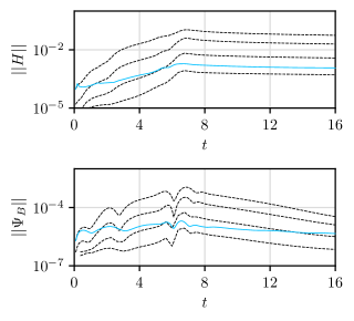
Figure 1: Convergence of $l_{2}$ norms of $\Psi_{B}$ and Hamiltonian constraint violations for strong field initial data given by Table 4. The plotted norms of the residuals for each run are evaluated by interpolating the results to a uniform grid which has sufficient resolution to resolve the details of the simulation. This enables us to directly compare the convergence properties at the various resolutions. Each of the dashed lines represents a successive refinement (by a factor of 2) of the initial data while the solid line represents an AMR run with a relative error tolerance of $5\cdot 10^{-5}$. The grid parameters for the various unigrid runs are given in Table 4.

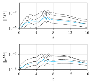
Figure 2: As Fig. 1 but for the convergence of the momentum constraints. Each of the dashed lines represents a successive refinement of the initial data while the solid line represents an AMR run with a relative error tolerance of $5\cdot 10^{-5}$.

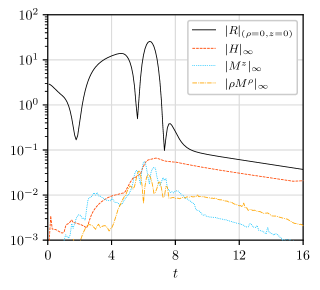
Figure 3: Magnitude of the 3D Ricci scalar, $R$, evaluated at $(0,0)$ and the $l_{\infty}$ norms of the Hamiltonian and momentum constraint violations for the AMR runs shown in Figs. 1 and 2. Post-dispersal, the solution becomes dominated by a non dispersing Hamiltonian constraint violation. Our critical search AMR simulations maintain constraint violations to about $1$ part in $500$ relative to the magnitude of the relevant fields throughout collapse.

V Results

V.1 Massless Scalar Field

We choose to include simulations of massless scalar field collapse in order to test the accuracy of our simulations and to verify the utility of our analysis methods. Extremely high accuracy numerical analysis of $\Delta$ have determined that, for the case of spherically symmetric critical collapse, $\Delta\approx 3.4454524022278213500$ [36, 4] while $\gamma\approx 0.37$ is known from simulations [3]. In this section, we verify that our simulations and analysis are of sufficient accuracy to reproduce these results.

As specified in Table 1, family $W_{l=0}$ is given by initially spherically symmetric initial data while family $W_{l=1}$ is initially a dipole. With family $W_{l=0}$, we demonstrate that our code is capable of resolving the spherically symmetric critical solution. By following the evolution of family $W_{l=1}$ we show that our code is capable of resolving situations where the initial data bifurcates into multiple on-axis centers of collapse. Since the results of Mendoza and Baumgarte demonstrated that quadrupole initial data was subject to such a bifurcation, we felt that it was important to validate our code in a similar regime. We have tuned these simulations to near the limits of double precision with $|p^{\star}-p|/p^{\star}\approx 1\cdot 10^{-15}$ for family $W_{l=0}$ and $|p^{\star}-p|/p^{\star}\approx 1\cdot 10^{-14}$ for family $W_{l=1}$.

Consider the proper time, $\tau$, of an inertial observer located at the accumulation point such that the observer would see the formation of a naked singularity at $\tau=\tau^{\star}$. The echoing period, $\Delta$, is then calculated using three somewhat independent methods. First, $\Delta_{1}$ is computed by taking the mean and standard deviation of the period between successive echoes at the center of collapse when viewed as a function of $-\ln\left(\tau^{\star}-\tau\right)$. Second, $\Delta_{2}$ comes from Fourier analysis of the dominant mode at the center of collapse in a similar frame. Third, $\Delta_{3}$ is calculated via the scaling relation (5), which results in an observer independent method given by

$$\Delta_{3} \approx\frac{\gamma}{N}\left(\ln\left|p_{1}-p^{\star}\right|-\ln\left|p_{2}-p^{\star}\right|\right)\,.$$ (80)

Here, $N$ is the number of echoing periods observed between simulations with family parameters $p_{1}$ and $p_{2}$, respectively. Table 5 summarizes the results using all three methods.

Plots of the lapse, $\alpha$, and the scalar field, $\mu$, as a function of logarithmic proper time evaluated at the approximate accumulation points are shown in Figs. 4 and 5 for families $W_{l=0}$ and $W_{l=1}$, respectively. Here, approximate accumulation points are defined as coordinate locations, $(z,\rho)$, of maximal scalar curvature encountered during the course of a subcritical simulation. These plots enable both direct and indirect calculation of $\Delta$ via the DSS time scaling relationship (3) and (80), respectively.

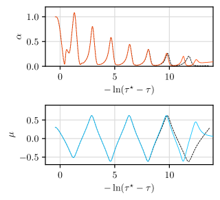
Figure 4: Lapse, $\alpha$, and value of the scalar field, $\mu$, as a function of $-\ln\left(\tau^{\star}-\tau\right)$ at the center of collapse (in this case the origin). Here, family $W_{l=0}$ data is used and both marginally subcritical (solid line) and supercritical (dashed line) solutions with $\left|{p^{\star}-p}\right|/{p^{\star}}\approx 1\cdot 10^{-15}$ are shown. Since the scalar field quickly approaches the critical solution with an associated strong-field scale that significantly decreases with each echo, we are able to accurately determine $\tau^{\star}$ to $\approx 1\cdot 10^{-6}$. Direct measurement of $\Delta$ from $\mu$ gives $\Delta_{1}=3.43(3)$, $\Delta_{2}=3.5(4)$ and $\Delta_{3}=3.6(4)$.

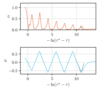
Figure 5: Lapse, $\alpha$, and value of the scalar field, $\mu$, as a function of $-\ln\left(\tau^{\star}-\tau\right)$ at the center of collapse (in this case $z\approx 0.594$). In this case family $W_{l=1}$ data is used and the marginally subcritical (solid line) and supercritical (dashed line) solutions have been determined to an overall accuracy of $\left|{p^{\star}-p}\right|/{p^{\star}}\approx 1\cdot 10^{-14}$. Here, $\tau^{\star}$ is computed to $\approx 1\cdot 10^{-5}$. Direct measurement of $\Delta$ from $\mu$ gives $\Delta_{1}=3.44(4)$, $\Delta_{2}=3.4(3)$ and $\Delta_{3}=3.2(4)$

Unlike the $W_{l=0}$ case, we find that for the family $W_{l=1}$, the solution bifurcates into two centers of collapse. This in turn makes the determination of the world line of the privileged observer non-trivial. As we are starting from time symmetric initial data, the ideal solution would be to integrate the world lines of a family of initially stationary observers and choose the one which was nearest the accumulation point at the closest approach to criticality. Unfortunately, our code is not currently set up to perform such an integration.

As a quick and potentially poor approximation, we choose the world line of an observer who remains at the approximate accumulation point throughout the evolution. This approximation is potentially error-prone because of its gauge dependence and the fact that the observer is generically non-inertial. However, for the case of the $W_{l=1}$ simulations, the solutions very quickly approaches two on-axis copies of the monopole solution so relatively little error appears to have been introduced by this choice.

The inverse Lyapunov exponent, $\gamma$, is calculated by fitting scaling laws of the form (6) for the maximal energy density, $\rho_{\mathrm{max}}$, and 3D Ricci scalar, $R_{\mathrm{max}}$, encountered during the course of a subcritical simulation. In these fits, we make the assumption that the dominant contribution to the putative universal periodic function is sinusoidal. As the specific region in parameter space where the scaling relationship is expected to hold is unknown (the uncertainty in $p^{\star}$ contaminates the values close to criticality, while radiation of dispersal modes contaminates the data far from criticality), we average a number of fits to reasonable subsets of the available data.

Ideally, we would calculate $\gamma$ via the maximal scale of some invariant quantity such as the 4D Ricci scalar (equivalently $\nabla_{\lambda}\mu\nabla^{\lambda}\mu$) or the Weyl scalar. However, calculations using frame dependent proxies such as the energy density, $\rho_{E}$, seem to be common in the literature and we have adopted this approach. In the case of collapse at the center of symmetry we note that $\rho_{E}$ is linearly related to the invariant $T$. Figs. 6 and 7 demonstrate the determination of $\gamma$ from $\rho_{E}$ and $R$ for families $W_{l=0}$ and $W_{l=1}$. Again, our results for $\gamma$ along with those for $\Delta_{1}$, $\Delta_{2}$ and $\Delta_{3}$ in the case of the scalar field are presented in Table 5.

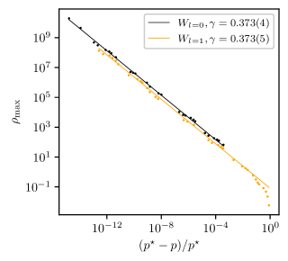
Figure 6: Inverse Lyapunov exponent, $\gamma$, determined via the scaling of the energy density $\rho_{E}$. Plotted here are the maximum values of $\rho_{E}$ obtained in each subcritical run as a function of $\left|{p^{\star}-p}\right|/{p^{\star}}$. The energy density has dimensions $M^{-2}$ and therefore scales according to $\left|p^{\star}-p\right|^{-2\gamma}$. Superior accuracy would be obtained by fitting to the maximum value of the 4D Ricci scalar or another invariant quantity. The lines represent an averaged fit to the underlying data.

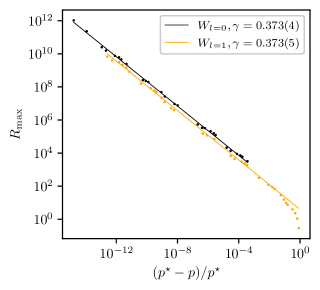
Figure 7: Inverse Lyapunov exponent, $\gamma$, determined via the scaling of the 3D Ricci scalar $R$. Plotted here are the maximum values of $R$ obtained in each subcritical run as a function of $\left|{p^{\star}-p}\right|/{p^{\star}}$. The Ricci scalar density has dimensions of $M^{-2}$ and therefore scales according to $\left|p^{\star}-p\right|^{-2\gamma}$. As in Fig. 6, the lines represent an averaged fit to the underlying data.

Family	$\Delta_{1}$	$\Delta_{2}$	$\Delta_{3}$	$\gamma$
$W_{l=0}$	$3.43(3)$	$3.5(4)$	$3.6(4)$	$0.373(4)$
$W_{l=1}$	$3.44(4)$	$3.4(3)$	$3.2(4)$	$0.373(5)$

Table 5: Estimated scaling exponents for axisymmetric scalar field collapse. The results summarized here agree with previous investigations to within the estimated error of our calculations. Although $\Delta_{3}$ is far less precisely determined than $\Delta_{1}$, it can be found in the absence of knowledge concerning a privileged inertial observer.

The excellent agreement between our computed values for the scaling exponents and previously established results for the massless scalar field demonstrate the accuracy of our simulations and the validity of our analysis. For AMR simulations, where it is impossible or impractical to establish the existence of convergence close to criticality, this process serves as an important verification and validation stage before the presentation of new results. It is worth noting that some previous studies [16, 2, 37] have presented evidence for a non-spherical unstable mode near criticality in scalar field collapse. We see no evidence for such a mode for either our $W_{l=0}$ or $W_{l=1}$ calculations, but have not examined this point in much detail.

V.2 Einstein-Maxwell System

With our methodology established and verified via investigation of the massless scalar field, the analysis of the critical collapse of the Einstein-Maxwell system proceeds in parallel fashion. We first consider the previously unstudied families $E_{l=1}$, $M_{l=1}$ and $M_{l=2}$ defined in Table 2. Once the behaviour of these solutions has been described, we turn our attention to the families of Table 3 which were originally studied by Baumgarte et al. [18], and Mendoza and Baumgarte [17]. In what follows, we define the approximate accumulation points as the coordinate locations of maximal $|F_{\mu\nu}F^{\mu\nu}|$ encountered during a subcritical run.

No bifurcations about the origin were observed for the dipole families $M_{l=1}$ and $E_{l=1}$: both families underwent collapse at the center of symmetry. Unfortunately, a gauge pathology prevented family $E_{l=1}$ from being investigated beyond $\left|{p^{\star}-p}\right|/{p}^{\star}\approx 5\cdot 10^{-9}$. This shortcoming seems to bear some resemblance to the sort of gauge problems encountered in evolving Brill waves towards criticality [10] and may be able to be resolved through the use of the shock avoiding gauge suggested by Alcubierre in [38] and successfully employed in [14, 15]. Fortunately, the pathology occurs sufficiently late in the evolution to enable the extraction of meaningful information concerning $\Delta$ and $\gamma$ for the family.

Figs. 8–9 plot $\alpha$ and $|F_{\mu\nu}F^{\mu\nu}|$ at the accumulation point (in this case the origin) versus $-\ln{\left(\tau^{\star}-\tau\right)}$ for near-critical evolutions of families $M_{l=1}$ and $E_{l=1}$. Since the collapse occurs at the center of symmetry, there is only a single accumulation point and the observers at the origin are privileged and inertial. As mentioned previously, this enables $\Delta$ to be accurately determined via statistical and Fourier analysis.

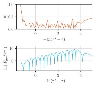
Figure 8: Lapse, $\alpha$, and invariant scalar, $\left|F_{\mu\nu}F^{\mu\nu}\right|$, at the center of collapse for family $M_{l=1}$ as a function of $-\ln\left(\tau^{\star}-\tau\right)$ for marginally subcritical (solid line) and supercritical (dashed line) solutions with $\left|p^{\star}-p\right|/p^{\star}\approx 1\cdot 10^{-13}$. Unlike the case of the scalar field, the strong-field scale of the critical solution only slowly decreases (i.e. $\Delta$ is small compared to the scalar case) and $\tau^{\star}$ can only be determined to a relative tolerance of about $10^{-4}$. Direct measurement of $\Delta$ from $F_{\mu\nu}F^{\mu\nu}$ gives $\Delta_{1}=0.64(2)$ via statistical analysis, $\Delta_{2}=0.63(3)$ via Fourier analysis and $\Delta_{3}=0.59(6)$ from (80).

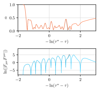
Figure 9: Lapse, $\alpha$, and invariant scalar, $\left|F_{\mu\nu}F^{\mu\nu}\right|$, at the center of collapse for family $E_{l=1}$ as a function of $-\ln\left(\tau^{\star}-\tau\right)$ for marginally subcritical (solid line) and supercritical (dashed line) solutions with $\left|p^{\star}-p\right|/p^{\star}\approx 1\cdot 10^{-9}$. As with family $M_{l=1}$, the strong-field scale of the critical solution slowly decreases and $\tau^{\star}$ can only be determined to a relative tolerance of about $10^{-3}$. Direct measurement of $\Delta$ from $F_{\mu\nu}F^{\mu\nu}$ gives $\Delta_{1}=0.65(3)$ via statistical analysis, $\Delta_{2}=0.65(4)$ via Fourier analysis, and $\Delta_{3}=0.67(8)$ from (80).

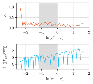
Figure 10: Lapse, $\alpha$, and invariant scalar, $\left|F_{\mu\nu}F^{\mu\nu}\right|$, at the center of collapse for family $M_{l=2}$ as a function of $-\ln\left(\tau^{\star}-\tau\right)$ with $\left|p^{\star}-p\right|/p^{\star}\approx 5\cdot 10^{-13}$. We use the proper time of a gauge dependent accelerated observer located at $z\approx 0.440$ as our independent variable, $\tau$, making the interpretation of length and time scales potentially problematic. It appears that the critical solution is divided into two separate regions (transition region shown in gray) with differing $\Delta$ and $\gamma$. A naive measurement of $\Delta$ under the assumption that our observer is approximately inertial gives $\Delta_{1}=0.30(2)$ and $\Delta_{2}=0.31(3)$ for the first region and $\Delta_{1}=0.56(3)$, $\Delta_{2}=0.63(6)$ for the second region. Application of (80) (which is valid irrespective of the status of the observer) gives $\Delta_{3}=0.19(4)$ for the first region and $\Delta_{3}=0.64(9)$ for the second The values of $\Delta_{2}$ and $\Delta_{3}$ measured in the second region as $p\rightarrow p^{\star}$ appear to be consistent with those found for families $E_{l=1}$ and $M_{l=1}$.

The analysis of family $M_{l=2}$ is both more interesting and more involved than that of families $M_{l=1}$ and $E_{l=1}$. In this case, and similarly to what is observed in the case of the massless scalar dipole, as the critical parameter is approached, the solution bifurcates into two on-axis centers of collapse. After this bifurcation the character of the critical solution changes markedly. Specifically, following this transition period, the growth and echoing period of the separated collapsing regions come to resemble those of two separated copies of the $M_{l=1}$ or $E_{l=1}$ critical solutions. This change in character is somewhat obscured in time series plots by the fact that we use the proper time of an accelerated observer at the accumulation point rather than that of a privileged inertial observer. Despite this, the change is evident in the growth rate, $\gamma$, when calculated via the scaling relationship

$$\ln{\left(|F_{\mu\nu}F^{\mu\nu}|_{\rm max}\right)} =-2\gamma\ln\left|p-p^{\star}\right|$$ (81)

$$\hphantom{=}+f_{F}\left(\gamma\ln\left|p-p^{\star}\right|\right)+c_{F},$$

as well as when $\Delta$ is calculated via (80). Overall, the two distinct phases of collapse can be seen in Figs. 10 and 11.

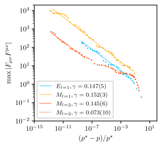
Figure 11: Inverse Lyapunov exponent, $\gamma$, determined via the scaling of the invariant scalar $\left|F_{\mu\nu}F^{\mu\nu}\right|$ which should scale as $\left|p^{\star}-p\right|^{-2\gamma}$. Plotted here are the maximum values of the invariant obtained in each subcritical run as a function of $\left|{p^{\star}-p}\right|/{p^{\star}}$. The lines shown are averaged fits of the underlying data and the quoted values of $\gamma$ are the slopes of those fits. As described in the text, fits to two distinct regions of family $M_{l=2}$ have been made.

Figure 11 shows the results of calculating $\gamma$ via the scalar invariant $F_{\mu\nu}F^{\mu\nu}$ which should scale as $\left|p^{\star}-p\right|^{-2\gamma}$ as in (81). Again, family $M_{l=2}$ appears to exhibit two distinct growth rates separated by a transition region in $\ln\left|p^{\star}-p\right|$. The early behaviour may be due to a slower growing quadrupole mode or perhaps simple radiation of initial data before the critical solution is approached. In total, the behaviour we observe appears to be consistent with the interpretation that, after the bifurcation occurs, the critical solution becomes dominated by the same mode as for families $M_{l=1}$ and $E_{l=1}$. A summary of our estimated values of $\Delta$ and $\gamma$ for the families defined in Table 2 is compiled in Table 6.

Family	$\Delta_{1}$	$\Delta_{2}$	$\Delta_{3}$	$\gamma$
$E_{l=1}$	$0.65(3)$	$0.65(4)$	$0.67(8)$	$0.147(5)$
$M_{l=1}$	$0.64(2)$	$0.63(3)$	$0.59(6)$	$0.152(3)$
$M_{l=2}$	$\mathbf{0.30(2)}$	$\mathbf{0.31(3)}$	$0.19(4)$	$0.073(10)$
$M_{l=2}$	$\mathbf{0.56(3)}$	$\mathbf{0.63(6)}$	$0.64(9)$	$0.145(6)$
$E_{\mathrm{quad}}$	$\bf{0.30(5)}$	$\bf{0.33(2)}$	$0.61(11)$	$0.164(19)$
$E_{\mathrm{quad}}$	$\bf{0.59(4)}$	$\bf{0.57(4)}$	$0.59(10)$	$0.152(20)$

Table 6: Summary of computed scaling exponents in critical collapse of the EM field for the families presented in Tables 2 and 3. The analysis of $E_{\mathrm{quad}}$ is presented in Section V.3. Here, the two separate rows for $M_{l=2}$ and $E_{\mathrm{quad}}$ denote fits to the distinct behavioral regions of the quadrupole solutions; the first row is for $p$ fairly distant from $p^{\star}$ while the second is for $p\rightarrow p^{\star}$. Results in bold indicate that the measurements were made using the world line of an accelerated observer and are unlikely to be accurate.

V.3 Direct Comparison to Previous Work.

When we compare our dipole and quadrupole results to those of Mendoza and Baumgarte [17] and Baumgarte et al. [18], the results are broadly consistent but do not fully agree to within our approximately determined errors. Although our work and the previous studies both indicate a single unstable mode with $\gamma_{l=1}\approx 0.15$ and $\Delta_{l=1}\approx 0.6$ for dipole type initial data, our investigation into an alternative family of quadrupole type initial data is consistent with a universal (rather than family dependent) growth rate and echoing period. In order to more conclusively determine the consistency of our work with that of [17] and [18], we attempt to replicate the previous computations by performing critical searches for the families listed in Table 3.

We perform evolutions of $E_{\mathrm{quad}}$ to a tolerance of $\lesssim 4\cdot 10^{-15}$ so as to resolve the critical solution as accurately as possible. Previously, this family was resolved to a relative tolerance of approximately $1\cdot 10^{-12}$ [17]. The evolutions for $E_{\mathrm{dipole}}$ were performed to a relative tolerance of only $\approx 1\cdot 10^{-4}$ and for the sole purpose of verifying that we had initial data consistent with [17].

Figure 12 directly compares our simulations to those of [17] using both our data and data provided by Mendoza and Baumgarte [39]. This figure plots the minimum value of $\alpha$ on each spatial slice for family $E_{\mathrm{quad}}$ for marginally subcritical simulations. Comparing our data, we observe a significant divergence at $\tau\approx 18$; earlier than would be expected based on the relative precision of our searches. Similarly, the scaling of Figs. 13–14 agree with Figs. 2 and 7 of Mendoza and Baumgarte [17] until $-\ln(\tau^{\star}-\tau)\approx 0$ and $|p-p^{\star}|/p^{\star}\approx 1\cdot 10^{-10}$ respectively. Past this point, the growth we observed increases relative to what was observed in [17].

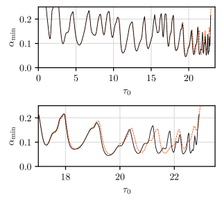
Figure 12: Minimum value of $\alpha$ on each spatial slice for family $E_{\mathrm{quad}}$ vs the proper time at the origin, $\tau_{0}$. The data plotted here represents the subcritical simulations closest to criticality for both our investigation (solid black line) and that of Mendoza and Baumgarte [17, 39] (dashed red line). The lower plot highlights the difference in behaviour at late times. Note that we have scaled $\tau_{0}$ for the data of Mendoza and Baumgarte by a factor of $\approx 1.003$ to better align the early minima and maxima of $\alpha_{0}$ with our own data. This degree of rescaling should be understood within the context of our simulations being only second order accurate and is performed to eliminate the dominant source of variation in our results far from the critical point. The simulations begin to differ markedly at $\tau\approx 18$, earlier than would be expected based on the relative precision of our searches.

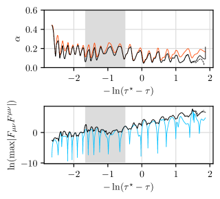
Figure 13: Lapse, $\alpha$, and invariant scalar, $\left|F_{\mu\nu}F^{\mu\nu}\right|$, at the center of collapse for family $E_{\mathrm{quad}}$ as a function of $-\ln\left(\tau^{\star}-\tau\right)$ for marginally subcritical (solid black line) and supercritical (dashed black line) solutions with $\left|p^{\star}-p\right|/p^{\star}\approx 4\cdot 10^{-15}$. Here, the black lines show the extremal values obtained on a spatial slice while the colored lines show the values at the center of collapse as determined by the coordinate location with largest value of $\left|F_{\mu\nu}F^{\mu\nu}\right|$ in the subcritical simulation closest to criticality.

Assuming that family $E_{\mathrm{quad}}$, like family $E_{l=2}$, is best described by dividing the near-critical evolution into early and late time behaviour, a naive measurement of $\Delta$ under the assumption that our observer at fixed coordinate location is approximately inertial, gives $\Delta_{1}=0.30(5)$, $\Delta_{2}=0.33(2)$ for the first region and $\Delta_{1}=0.59(4)$, $\Delta_{2}=0.57(4)$ for the second region. Application of (80) gives $\Delta_{3}=0.61(11)$ for the first region and $\Delta_{3}=0.59(10)$ for the second. The large discrepancy between the values of $\Delta$ computed in the first region likely indicates that the solution does not show DSS behaviour far from criticality.

Fig. 14 plots $\left|F_{\mu\nu}F^{\mu\nu}\right|$ as a function of $\left|{p^{\star}-p}\right|/{p^{\star}}$ and is used to determine $\gamma_{\mathrm{quad}}=0.152(20)$. This in turn is consistent with the values of $\gamma$ determined for all other families. It is clear that the early behaviour of family $E_{\mathrm{quad}}$ is very different from that of family $M_{l=2}$, which indicates that the early scaling behaviour observed for both families may simply be the result of radiation of features of the initial data on the path to criticality. Again we note that we list the complete set of $\Delta$ and $\gamma$ for family $E_{\mathrm{quad}}$ as well as for the families defined in Table 2 in Table 6 of the previous section.

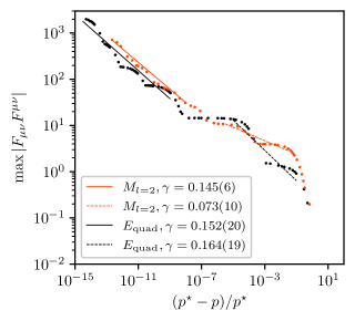
Figure 14: $\gamma$ determined via the scaling of the invariant scalar $\left|F_{\mu\nu}F^{\mu\nu}\right|$ which should scale as $\left|p^{\star}-p\right|^{-2\gamma}$. Plotted here are the maximum values of $\left|F_{\mu\nu}F^{\mu\nu}\right|$ obtained in each subcritical run as a function of $\left|{p^{\star}-p}\right|/{p^{\star}}$. It is apparent that although both quadrupole solutions exhibit scaling with similar $\gamma$ close to criticality the initial behaviour is highly family dependent.

It is apparent that, close to criticality, the growth rates and echoing periods we observe for family $E_{\mathrm{quad}}$ differ markedly from those observed in [17]. Assuming that our results are correct, we hypothesise that the use of spherical polar coordinates with limited resolution in $\theta$ [17] may have had the inadvertent effect of leaving insufficient resolution to resolve dipole collapse away from the center of symmetry. If this is the case, then it is plausible that the growth of the dipole mode was suppressed in a manner similar to what is apparently observed.

VI Summary and Conclusions

We have investigated the critical collapse of both the massless scalar field and the Maxwell field in axisymmetry using the GBSSN formulation of general relativity. Our study of the scalar field was largely motivated by the need to calibrate our numerical methods—including AMR—and to develop analysis procedures. Nonetheless we are able to reproduce previous results on massless scalar collapse to the estimated accuracy of our calculations. Moreover, in contrast to some other earlier work [37, 16, 2], we find no evidence of non-spherical unstable modes at criticality. However, as we have not examined this issue very closely we feel that it is well worth further study.

With regard to the Einstein-Maxwell system, we observe that for generic initial data a dipole mode with $\gamma_{l=1}\approx 0.149(9)$ and $\Delta_{l=1}\approx 0.62(8)$ seems to be dominant. If there is an unstable quadrupolar mode, variations between the families $M_{l=2}$ and $E_{\mathrm{quad}}$ of Tables 2 and 3 suggest that it is not universal.

We observe significant differences in the behaviour of family $E_{\mathrm{quad}}$ close to criticality relative to the results reported in [17], although our findings appear largely similar until $\left|p^{\star}-p\right|/p^{\star}\approx 1\cdot 10^{-10}$. We hypothesize that these differences may be due to the inability of spherical coordinates to fully resolve off-center collapse when limited angular resolution is employed.

The observed consistency between $\gamma$ and $\Delta$ for each of the families in conjunction with the observed variance in the form of $f(x)$ (seen in Figs. 11 and 14) and absence of perfect DSS (seen in Figs. 8–10 and Fig. 13) is puzzling and requires additional study. Conservatively, it could be that given the slow growth rate of the dipolar critical solution, our simulations have simply not radiated away all traces of their initial data and this manifests in the apparent inconsistency of $f(x)$.